Consistent generation of magnetic fields in axion inflation models

Magnetic fields are observed on many different scales in our universe. In particular, it has been known that galaxies and galaxy clusters have their own magnetic fields with the typical strength, $10^{-6}{\rm G}$ [1, 2, 3, 4, 5]. Although their existence is observationally confirmed, the origin of these magnetic fields is still one of the open questions in cosmology. Recently, the gamma-ray observations from blazars suggest the existence of cosmological magnetic fields even in voids [6, 7, 8, 9, 10, 11, 12, 13]. They set the lower bound on the effective strength of the void magnetic fields, given as [10, 14]

where $B$ is the present field amplitude with the correlation length $\lambda$.¹¹ 1 If one assumes that the suppression of the cascade emission is caused by the time delay of the cascade photons, one obtains a more conservative bound as $B_{\rm eff}\gtrsim 10^{-17}$ [10]. The recent simulation indicates that if magnetic fields whose comoving strength is larger than $10^{-19}{\rm G}$ exist prior to galaxy formation, they can be amplified to $10^{-6}{\rm G}$ as the disk of galaxy develops [15]. Therefore the reported magnetic fields in voids can seed those in galaxies and galaxy clusters. Hence “primordial magnetogenesis” can be a key ingredient of cosmology to explain the existence of magnetic fields in both galactic and extragalactic scales.

Magnetogenesis during inflation has attracted attention, and many models have been proposed so far [16, 17, 18, 19, 20, 21, 22, 23, 24, 25, 26, 27, 28, 29, 30] (see also ref. [31]). In such scenarios, large-scale magnetic fields are expected to be generated during inflation via its causal production of fluctuations. Recently, however, the obstacles of inflationary magnetogenesis have been recognized, and it is understood to be quite difficult to generate magnetic fields only during inflation with the field strength satisfying the observational lower bound given by eq. (1) [32, 33, 34, 35, 36, 37]. Since magnetic fields are substantially diluted after inflation due to the cosmic expansion, their energy density needs to be extremely large during inflation, altering the inflation dynamics and/or inducing an additional curvature perturbation which exceeds the observed value in the cosmic microwave background (CMB) radiation [38]. Thus inflationary magnetogenesis faces three obstacles: (i) substantial dilution of the produced magnetic fields after inflation, (ii) too large electromagnetic energy spoiling inflation itself, and (iii) induced curvature perturbations being inconsistent with the CMB observation.

In this paper, to overcome these three obstacles, we consider the axial coupling model in which a (pseudo-)scalar field $\phi$ is coupled to the electromagnetism through a term, $\phi F^{\mu\nu}\tilde{F}_{\mu\nu}$, where $F_{\mu\nu}$ is the field strength tensor of the $U(1)$ gauge field, and $\tilde{F}_{\mu\nu}$ is its dual. This coupling naturally arises under symmetries as the leading interaction of a pseudo-scalar and excites either of the left- or right-handed polarization modes of the gauge field. Helical magnetic fields, which are characterized by an imbalance between their two polarization states, have an interesting feature that part of its energy on small scales is transferred to that on large scales by non-linear effects of turbulent plasma with a high electric conductivity. This phenomenon is called the inverse cascade process. In practice, this process amplifies the comoving amplitudes of helical magnetic fields on large scales, and, as a result, their characteristic scale can grow. Therefore it can alleviate the substantial dilution of such magnetic fields on large scales in the cosmological context [39, 40]. Recently, the possible signatures of cosmological helical magnetic fields are reported in ref. [41, 42].

In the previous works on the axial coupling models, only the slow-roll regime of $\phi$ was considered [18, 24, 26, 27]. To evaluate the generated magnetic fields, they applied an approximated analytic solution of the gauge field which is valid only during the slow roll regime without its backreaction onto the inflationary dynamics. However, we find that the generation of the electromagnetic fields is much more efficient at the end of the slow-roll regime and during the subsequent oscillation phase of $\phi$. Since the slow-roll approximation is no longer valid in these regimes, we numerically solve the equations of motion of these fields, consistently taking into account the backreaction from the gauge field to the dynamics of $\phi$ and the background expansion. As a result, much stronger magnetic fields can be obtained than the ones in the preceding studies with the same setup [18, 24].

In our scenario, the electromagnetic fields are mainly generated right after the end of inflation, and hence we do not need to worry about the electromagnetic energy density spoiling inflation. Furthermore, since the peak scales of the produced magnetic fields are far smaller than the CMB scales, they are free from the CMB constraints. Therefore our scenario overcomes the three obstacles of inflationary magnetogenesis, and relatively strong magnetic fields can be generated. Unfortunately, however, in the case where $\phi$ is the inflaton in large-field models, the strength of the resultant magnetic fields does not reach the observational bound, eq. (1), by a few orders of magnitude.

Two additional issues concern us in the scenario. One is the effect of electrically charged particles. We investigate the generation of magnetic fields by solving the coupled system of the background inflaton and the gauge field. However, if a sufficient amount of charged particles are present at the time of the magnetic field production, they may change the dynamics of the gauge field in a non-trivial way [43]. To avoid such cumbersome complexity, we require the inflaton decay rate is suppressed such that the charged particles are negligible during the production period. Nonetheless, since the reheating is delayed, the dilution of the produced magnetic field before the onset of the inverse cascade process is inevitably significant. The other issue is the non-linear effect of the axial coupling on the dynamics of the inflaton and of the gauge field. With this non-linear interaction taken into account, the gauge field produced by the background inflaton inverse-decays to the inflaton’s fluctuations, which then in turn produces the gauge field. For the large value of the axial coupling constant, this successive non-linear process would change the dynamics of the inflaton and gauge field as shown in ref. [44]. Since fully handling the non-linear dynamics requires lattice simulations, we only consider the coupling constant small enough to ignore the effect of the inflaton perturbation on the gauge field dynamics.

The rest of this paper is organized as follows. In sec. 2, we introduce our setup and review the approximated solution for the gauge field in the slow-roll regime. In sec. 3, we show the result of our numerical calculation and describe the dynamics of the model. In sec. 4, we take into account the inverse cascade process as the conservation of the helicity of the produced magnetic fields. Following the evolution after reheating, we exhibit the computation of the present values of the field strength and the correlation length for a given coupling constant in the model. In sec. 5, we discuss the effects of charged particles on reheating in various cases. In sec. 6, the amount of the inflaton perturbation generated by the inverse-decay of the gauge quanta is evaluated, and the strongest reliable value of the effective magnetic field strength in our frame work is presented. Finally we conclude in sec. 7.

In this paper we consider the axial coupling model with the following Lagrangian:

where $\phi$ is the inflaton,$F_{\mu\nu}\equiv\partial_{\mu}A_{\nu}-\partial_{\nu}A_{\mu}$ is the field strength tensor of the $U(1)$ gauge field $A_{\mu}$, and $\tilde{F}^{\mu\nu}\equiv\epsilon^{\mu\nu\rho\sigma}F_{\rho\sigma}/\left(2\sqrt{-g}\right)$ is its dual. Inspired by the axion case in which $\phi$ is a pseudo-Nambu-Goldstone boson coupled to the axial vector current of charged fermions and the $\phi F\tilde{F}$ coupling arises from the chiral anomaly, we introduce the coupling constant as $\alpha/f$ where $\alpha$ is a dimensionless constant and $f$ corresponds to the axion decay constant. However, since this coupling is realized simply by symmetry consideration, we concentrate on phenomenology of the above Lagrangian without assuming any particular particle physics model. For simplicity, the potential is assumed to be quadratic form,²² 2 The recent Planck result [45] disfavors the quadratic potential of inflaton. In this work, however, we use it as an example to depict the consistent generation and evolution of the magnetic fields from the $\phi F\tilde{F}$ term. Moreover, as we will show later, the dominant contribution to the magnetic fields in this model comes from the modes that cross the horizon near the end of inflation, and their amplification due to parametric resonance occurs during the early stage of inflaton oscillation. During this period, the quadratic potential is expected to be a good approximation of less simple forms, justifying its use.

In the flat FRW universe with the Einstein gravity, one can derive the equations of motion for the background inflaton $\phi_{0}(t)$ and the mode function of the gauge field $\mathcal{A}_{\pm}(k,t)$ as [46]

with

where the overdot denotes the cosmic time derivative, and $a$ is the scale factor. In this paper, we take the Coulomb gauge, $A_{0}=\partial_{i}A_{i}=0$. We decompose and quantize the gauge field as

where $e^{(\pm)}_{i}(\hat{\bm{k}})$ are the right/left-handed polarization vectors which satisfy $\epsilon_{ijl}k_{j}e_{l}^{(\pm)}(\hat{\bm{k}})=\mp ike_{i}^{(\pm)}(\hat{\bm{k}})$, and $a_{\bm{k}}^{(\pm){\dagger}},a_{\bm{k}}^{(\pm)}$ are the creation/annihilation operators which satisfy the usual commutation relation, $[a^{(\lambda)}_{\bm{k}},a^{(\sigma){\dagger}}_{-\bm{k}^{\prime}}]=(2\pi)^{3}\delta(\bm{k}+\bm{k}^{\prime})\delta^{\lambda\sigma}$. With the definition of the electric and magnetic fields in terms of the gauge field, $E_{i}\equiv-a^{-1}\partial_{t}A_{i}$ and $B_{i}\equiv a^{-2}\epsilon_{ijk}\partial_{j}A_{k}$, one can derive eq. (6).

Eq. (5) implies that either of two polarization modes $\mathcal{A}_{\pm}$ has the tachyonic instability for $k/a<\alpha|\dot{\phi}_{0}|/f$, depending on the sign of $\dot{\phi}_{0}$. Thus the gauge fields are produced at the expense of the time kinetic energy of $\phi_{0}$. The term on the right hand side in eq. (4) represents the backreaction from the gauge field to the inflaton and it slows down the motion of $\phi_{0}$. It should be noted that the perturbation of the inflaton, $\delta\phi(t,\bm{x})$, is ignored in the above set of equations. We discuss the validity of this assumption in sec. 6.

Before exploring our scenario with the full numerical calculation, it is instructive to review the gauge field production in the slow-roll regime of $\phi$. For this purpose, it is useful to introduce a new parameter $\xi$ as

where $H$ is the Hubble parameter. With the conformal time $\eta$, eq. (5) is rewritten as

When $\xi$ is constant which is a good approximation in the slow-roll regime, the exact solution of this equation is available. If $\dot{\phi_{0}}<0$, then $\xi<0$ and the $(-)$ mode has the tachyonic instability. With the adiabatic initial condition,

in the sub-horizon limit, one finds the analytic solution and the asymptotic expression for the growing $(-)$ mode are given by

up to an irrelevant constant phase, where $F_{L}(\kappa,z)$ and $G_{L}(\kappa,z)$ are regular and irregular Coulomb wave functions, respectively. Therefore the growing mode is amplified by a factor $e^{\pi|\xi|}/\sqrt{2\pi|\xi|}$ due to the tachyonic instability. Since the produced gauge field induces non-gaussian perturbations of the inflaton, $\delta\phi$, the value of $\xi$ at the horizon-crossing of the CMB mode ($k_{*}=0.002{\rm Mpc}^{-1}$) is constrained as $|\xi_{*}|<2.37$ [47]. At smaller scales, non-detection of primordial black holes (PBHs) can potentially push the constraint further down [48]. While the constraint from PBHs inherits uncertainty, the forthcoming generations of terrestrial gravitational-wave (GW) detectors can directly probe the GWs sourced by the produced gauge field. It has been demonstrated that, for a quadratic potential of inflaton $\phi$, the second-generation detectors (Advanced LIGO, VIRGO, and KAGRA) will be able to probe $|\xi_{*}|\gtrsim 2.2$ (at $95\%$ CL, based on flat priors on $\xi$) and the third-generation experiments can improve the sensitivity to $|\xi_{*}|\gtrsim 1.9$ [49, 50].

Since the gauge field production is characterized by $|\xi|$, it is expected that the generation of the gauge fields is the most efficient when $|\xi|$ reaches its maximum value. Indeed, $\xi\propto\dot{\phi}_{0}/H\simeq-2M_{\rm Pl}^{2}/\phi_{0}$ in the slow-roll regime, and its absolute value increases during inflation. In fig. 1, we plot the evolution of $\dot{\phi}_{0}/H\propto\xi$.

One can see that $|\xi|$ increases during inflation and reaches its maximum value when $\phi_{0}$ crosses its origin at $N\approx 0.5$ after inflation. It then starts to oscillate with a large amplitude in the oscillation phase. Thus, in order to evaluate the produced magnetic field, one has to investigate the dynamics after inflation, the period during which the analytic solution is no longer valid. It seems that this critical point is overlooked in the previous works [18, 24, 26, 27]. Note that the amplitude of $\xi$ slightly decreases and the oscillation phase changes for $N\gtrsim 1.5$ in the case with $\alpha M_{\rm Pl}/f=8,$ because of the backreaction from the gauge field (compare the two lines in fig. 1).

By a numerical calculation, we simultaneously solve eqs. (4), (5) and the Friedmann equation,

where $M_{\rm Pl}$ is the reduced Planck mass, and the energy density of electromagnetic fields $\rho_{\rm em}$ is given in terms of the mode function of the gauge field $\mathcal{A}_{\pm}(k,t)$ as

However, since the gauge field is solved in Fourier space, and $\langle\bm{E}\cdot\bm{B}\rangle$ and $\rho_{\rm em}$ contain the momentum integrations, we have to solve eq. (5) for many modes of $\mathcal{A}_{\pm}(k,t)$ with different wave numbers simultaneously. In our numerical calculation, we start to solve for a mode function $\mathcal{A}_{\pm}(k,t)$ with the initial condition eq. (10), when its wave number equals to a rapidly growing function, $100k_{\rm ins}(t)$, where $k_{\rm ins}\equiv\alpha a\dot{\phi}/f=2\xi aH$ is the wave number for which the $(-)$ mode becomes unstable, and continue to solve the mode until the end of calculation. In other words, we solve for all modes which satisfy $100k_{\rm ins}(t_{i})<k<100k_{\rm ins}^{\rm max}(t)$, where $t_{i}$ is the onset of the calculation, $N(t_{i})\approx-70$, and $k_{\rm ins}^{\rm max}(t)$ is the maximum value of $k_{\rm ins}$ on the interval $[t_{i},t]$. The grid size of the wave number is set as $\delta\ln k=0.01.$ To eliminate the contribution from the modes in the vacuum state, we do not integrate all the modes being solved in eqs. (6) and (13) but only the modes satisfying $k<k_{\rm ins}(t)$ at least once during the numerical evolution. For confirmation, we check another criterion. We integrate only the modes with a sufficient amplitude, $|\sqrt{2k}\mathcal{A}_{\pm}|>20$, and compare the result with that of the former criterion, confirming no recognizable change. The time step of the numerical calculation is set as $\delta t=10^{-4}a(t)/k_{\rm ins}(t)$, which is always much shorter than the inflaton oscillation time scale, $m^{-1}$. We check the total energy conservation, $\dot{\rho}=-3H(\rho+p)$, is satisfied in sub-percent accuracy.

In this section, we discuss only the case of $\alpha M_{\rm Pl}/f=8$, because it is close to the maximum value of the coupling constant $\alpha M_{\rm Pl}/f$ for which our treatment is justified. For larger $\alpha M_{\rm Pl}/f$, we need to take into account the inflaton perturbation induced by the gauge field. However, it requires lattice simulations as the re-scattering process between the gauge field $\mathcal{A}_{\pm}$ and $\delta\phi$ is fully non-linear. Thus in this paper, we only consider the case where the coupling is not too strong and the inflaton perturbation is negligible, $\delta\phi\ll\phi_{0}$. We will discuss this point with more detail in sec 6.

Let us now show the result of our numerical calculation.

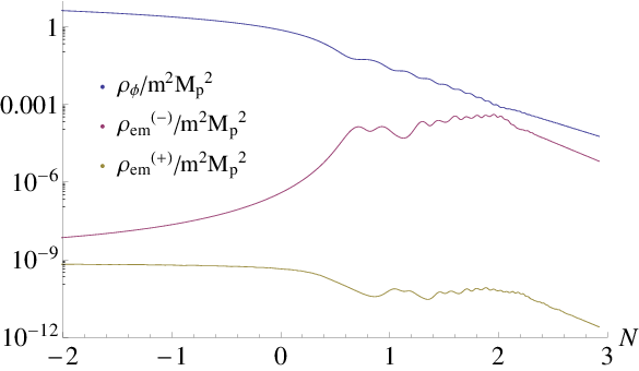
In fig. 2, we plot the energy density of the inflaton and the two polarization mode of the gauge field in the left panel. The horizontal axis $N$ denotes the e-fold number, and inflation ends at $N=0$. One can clearly see that the electromagnetic fields are mainly generated after inflation and the energy density $\rho_{\rm em}=\rho_{\rm em}^{(-)}+\rho_{\rm em}^{(+)}$ reaches its maximum value at 2 e-folds after the end of inflation. Note that $\rho_{\rm em}$ is always dominated by the contribution from the $(-)$ mode $\rho_{\rm em}^{(-)}$. Until $N\simeq 0.75$, $\dot{\phi}$ is negative (see fig. 1), and only the $(-)$ mode of the gauge field continues to grow due to the tachyonic instability. However, after the sign of $\dot{\phi}$ changes, the $(-)$ mode transiently decreases due to acquiring a positive mass, while the $(+)$ mode begins to increase by the tachyonic instability in turn. Subsequently, the inflaton oscillation develops, and the parametric resonance becomes efficient. Although not only $\mathcal{A}_{-}$ but also $\mathcal{A}_{+}$ is amplified in this regime, $\mathcal{A}_{-}$ is far larger than $\mathcal{A}_{+}$ due to the initial hierarchy implemented by the tachyonic instability, and thus a helical magnetic field is generated. As the amplitude of the inflaton oscillation decreases, the efficient resonance eventually terminates. After that, since the inflaton and the gauge field are now decoupled, they behave as the usual matter and radiation components, respectively.

In the right panel of fig. 2, the potential force of the inflaton $V^{\prime}\equiv\partial V/\partial\phi=m^{2}\phi$ and the backreaction from the gauge field to the inflaton $\alpha\langle\bm{E}\cdot\bm{B}\rangle/f$ are shown. Although the backreaction term is always subdominant in this case of $\alpha M_{\rm Pl}/f=8$, it becomes non-negligible and the behavior of $\phi$ is significantly affected for a larger coupling constant.

In fig. 3, we show the spectra of the mode function $\mathcal{A}_{\pm}(k,t)$. Although $\mathcal{A}_{+}$ does not have the tachyonic instability during inflation, the oscillating inflaton amplifies $\mathcal{A}_{+}$ to at most $\mathcal{O}(10^{2})$ through the parametric resonance as the oscillating behavior of the spectrum indicates. The mode $\mathcal{A}_{-}$ acquires the double amplification both from the tachyonic instability and the parametric resonance, and the peak mode at $k/a_{f}\sim 0.1m$ undergoes the $\mathcal{O}(10^{5})$ amplification. It corresponds to $|\xi|\approx 4.5$ in the constant $\xi$ case, while $\xi$ at the horizon crossing of the CMB scale is $|\xi|\simeq\alpha M_{\rm Pl}/2\sqrt{4N_{\rm CMB}+2}f\approx 0.3$ in this setup. It should be noted that since $\mathcal{A}_{-}$ is much larger than $\mathcal{A}_{+}$ at the end, an almost maximal helical magnetic field is eventually generated (see eq. (18)).

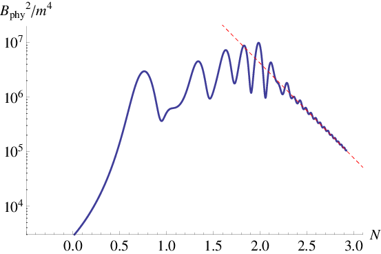
Following refs. [40, 27], we define the physical intensity and the physical correlation length of the magnetic field as

In fig. 4, we plot them as a function of the e-fold number $N$ for $\alpha M_{\rm Pl}/f=8$. After the coupling between the inflaton and the gauge field becomes ineffective ($N\gtrsim 2$), the electromagnetic fields effectively satisfy the free wave equation, $[\partial_{\eta}^{2}+k^{2}]\mathcal{A}_{\pm}(k,\eta)=0$, and thus $|\mathcal{A}_{\pm}|$ become constant. Then we can fit the numerical result as (see the red dashed lines in fig. 4.)

By using the fitted behavior of the Hubble parameter, $H\simeq 0.36me^{-3N/2}$, and the unit conversions $1{\rm G}=6.8\times 10^{-20}{\rm GeV}^{2}$ and $1{\rm GeV}^{-1}=6.4\times 10^{-39}{\rm Mpc}$, one can rewrite eq. (16) as

This is the physical magnetic field amplitude with the associated correlation length after all the production processes complete, and this behavior continues to hold until charged particles are generated by the inflaton decay. Thereafter the produced helical magnetic field undergoes the inverse cascade process.

As the inflaton decays and particles in the standard model appear, the electric conductivity $\sigma_{c}$ increases. The conductivity gives a friction term in the equation of $\mathcal{A}_{\pm}$ as $[\partial_{t}^{2}+(H+\sigma_{c})\partial_{t}+k^{2}/a^{2}]\mathcal{A}_{\pm}=0$. Since, after the reheating completes, the conductivity of the thermalized plasma exceeds the Hubble parameter, $\sigma_{c}\gg H$, one can find that on large scales $k\ll a\sqrt{\sigma_{c}H}$ the gauge mode functions freeze, $\mathcal{A}_{\pm}\simeq const.$ [25]. Thus the corresponding electric fields vanish, and the static magnetic fields which merely dilute due to the cosmic expansion remain on such large scales. On small scales, the evolution of magnetic fields is different due to the nonlinearity of the fluid dynamics [39, 40]. Turbulence in a plasma induced by the Lorentz force highly develops on small scales. The turbulence transfers the energy of the magnetic fields from large scales to small scales due to a non-linear interaction between the plasma fluid and the magnetic fields. This is called the direct cascade process. The resultant spectrum of the magnetic field is red-tilted on small scales where the time scale of the turbulence is smaller than the cosmological time scale.

However, when a magnetic field is helical, not all of its energy is transferred to small scales. According to Maxwell equations, the magnetic helicity should be conserved in the magnetized plasma with a high conductivity. Therefore, in order to maintain the helicity, a part of the energy is transferred to a slightly larger scales where the turbulence does not develop well. This is called the inverse cascade process.

The magnetic helicity $\mathcal{H}$ is defined as $\mathcal{H}\equiv\int_{V}\mathrm{d}^{3}x\epsilon_{ijk}A_{i}\partial_{j}A_{k}$ where the spacial integral is taken over a finite comoving volume $V$ on which magnetic fields have no component normal to the boundary, i.e. $\bm{B}\cdot\bm{n}=0$. Then $\mathcal{H}$ is invariant under the gauge transformation (see e.g. [51]). With eq. (7), the expectation value of the helicity density $\mathfrak{h}$ which is defined as $\mathfrak{h}\equiv\mathcal{H}/V$ is given by

Thus the helicity density represents the difference between the left-handed and the right-handed polarization modes. When a magnetic field is perfectly helical (i.e. one component of polarization modes is non-zero while the other components are zero), the helicity conservation, $\mathcal{H}=const.$ or equivalently $\mathfrak{h}=const.$, provides the constraint between the strength and the correlation length of the helical magnetic field as

It is clear that this equation holds for freezed magnetic fields because their physical scale and strength simply evolved as $\lambda_{\rm phy}(t)\propto a$ and $B_{\rm phy}(t)\propto a^{-2}$. However this equation is valid even in the turbulent regime where the magnetic field evolution is affected by the turbulence in a plasma and $\lambda_{\rm phy}$ grows faster than $a$. The scale and strength of magnetic fields in the turbulent regime evolve with satisfying this equation.

The study about the evolution of magnetic fields with non-zero helicity after inflation requires a MHD numerical simulation. However the helicity conservation enable us to directly compare helical magnetic fields produced in early universe with the observation bound by using eq. (19), because the constraint from blazar observations, eq. (1), is proportional to $\lambda_{\rm phy}B_{\rm phy}^{2}\propto\langle\mathfrak{h}\rangle$ for magnetic fields with $\lambda<1~{\rm Mpc}$. The scale factor at the completion of reheating is given by

where $\Gamma_{\phi}$ is the decay rate of the inflaton, and we set the scale factor at present as unity. Therefore, when the helicity conservation is valid, the effective strength of the helical magnetic field at present can be written as

where $t_{\rm reh}$ denotes the time at the reheating completion. Recall $B_{\rm eff}$ is defined in eq. (1). Substituting eq. (17) with $H=\Gamma_{\phi}$, we finally obtain the produced $B_{\rm eff}$ at the present epoch in the case of $\alpha M_{\rm Pl}/f=8$ as

In the next section, we discuss the allowed values of $\Gamma_{\phi}$. Furthermore, in sec. 6, we explore the larger values of the coupling constant $\alpha/f$. There exists the parameter space where the stronger $B_{\rm eff}$ is obtained.

Although, with the helicity conservation, we can estimate $B_{\rm eff}$ at present from the strength and scale of a helical magnetic field at the reheating epoch, $B_{\rm phy}(t)$ and $\lambda_{\rm phy}(t)$ are degenerate in $B_{\rm eff}$. Before closing this section, we explore the way to resolve the degeneracy between $B_{\rm phy}(t)$ and $\lambda_{\rm phy}(t)$.

If the initial spectrum of the helical magnetic fields is blue-tilted, as in the present case, its characteristic length scale, at which most of the magnetic field energy resides, is shifted to the scale comparable to that of the turbulence, $\lambda_{T}(t)$. This is due to the direct cascade process, in which the magnetic field energy on the scales smaller than $\lambda_{T}(t)$ is significantly transferred by the turbulence to farther smaller scales and dissipates away.

The turbulence scale $\lambda_{T}$ is given by the plasma fluid velocity $v$ and the cosmic time $t$ as $\lambda_{T}(t)\sim vt$. When the turbulence fully develops, the equipartition state between the fluid and the magnetic field is achieved. In that case, $v$ reaches the Alfvén velocity, $v_{A}(t)\simeq B_{\rm phy}/\sqrt{\rho}$, where $\rho$ is the energy density of the plasma. Thus one finds $\lambda_{\rm phy}\sim tB_{\rm phy}/\sqrt{\rho}.$ This equation holds until the recombination when most of the charged particles disappears and the turbulence terminates (see also refs. [39, 40] for a more detailed discussion). After that, $B_{\rm phy}$ and $\lambda_{\rm phy}$ evolve as usual, only due to the cosmological expansion, $B_{\rm phy}\propto a^{-2},\lambda_{\rm phy}\propto a$. ³³ 3 Since residual charged particles remain after the recombination, the MHD interaction is effective between the magnetic fields and the plasma fluid. However, since the Alfvén velocity is proportional to $a^{-1/2}$ in the matter dominated plasma, $tv_{A}$ evolves as $\propto a$. Therefore, the MHD interaction in the matter dominated era does not induce the further evolution of $\lambda_{\rm phy}/a$. Thus, $B_{\rm phy}/\lambda_{\rm phy}$ at present is given by

where the subscript “rec” denotes the recombination and $T_{\rm CMB}\approx 3$K. Therefore, we obtain [39, 40]

Combining this equation and the helicity conservation, one can solve for each of $B_{\rm phy}$ and $\lambda_{\rm phy}$ at present as

Substituting eq. (17) with $H=\Gamma_{\phi}$, we find

The MHD numerical simulations in ref. [39, 53, 54] show that, due to the inverse cascade, the spectral index of the magnetic field energy spectrum, ${\cal P}_{B}$, is $\sim 5$ on the scales larger than the peak scale. Therefore, the magnetic field strength at the scale $L$ ($L>\lambda_{\rm phy}$) is roughly evaluated as $B_{L}\sim B_{\rm phy}(\lambda_{\rm phy}/L)^{5/2}$.

Provided that reheating proceeds instantaneously and charged particles appear at once, one can substitute eq. (17) with $H=\Gamma_{\phi}$ into eq. (21) independently on the value of $\Gamma_{\phi}$, (if $\lambda<1{\rm Mpc}$ and $\Gamma_{\rm reh}\lesssim 10^{-2}m$). However, charged particles can be produced before the completion of reheating, $H=\Gamma_{\phi}$, since the inflaton decay is active even for $H>\Gamma_{\phi}$. For example, by assuming the inflaton decay rate $\Gamma_{\phi}$ is constant and the energy density of the decay products $\rho_{\rm rad}(t)$ satisfies, $\dot{\rho}_{\rm rad}+4H\rho_{\rm rad}=\Gamma_{\phi}\rho_{\phi}$, one finds $\rho_{\rm rad}=2\Gamma_{\phi}\rho_{\phi}/5H$ in the inflaton oscillating phase [52]. Thus the decay products occupy roughly $\Gamma_{\phi}/H$ of the total energy density. If the charged particles in $\rho_{\rm rad}$ affected the dynamics of $\mathcal{A}_{\pm}$ before the decoupling between the inflaton and the gauge field, we would have to reconsider the result in sec. 3, which does not take into account the effect of the charged particles.⁴⁴ 4 In ref. [43], the authors study how the growing electric conductivity suppresses the generation of magnetic fields by a parametric resonance, while they assume different couplings, $\phi^{2}A^{2}$ and $RA^{2}$, from ours. Therefore in this section, we discuss the maximum value of $\Gamma_{\phi}$ for which our numerical result in sec. 3 is verified.

In sec. 3, we focus on the case of $\alpha M_{\rm Pl}/f=8$. One expects if the coupling constant is larger, stronger magnetic fields are produced. However, at the same time, one should care about the consistency of the assumption, $\delta\phi\ll\phi_{0}$, which we made in the equation of motion for the gauge field, eq. (5). If the coupling between the inflaton and the gauge field is too strong, the perturbation of the inflaton $\delta\phi$ is significantly produced by the gauge field and $\delta\phi$ becomes non-negligible compared to $\phi_{0}$. Then $\delta\phi$ potentially alters the production of the gauge field, while it is difficult to take into account the non-linear coupling between $\delta\phi$ and $\mathcal{A}_{\pm}$ without performing full lattice simulations. To find the allowed maximum value of the coupling constant where our assumption is valid, we evaluate the variance of the inflaton perturbation $\langle\delta\phi^{2}\rangle$ by ignoring the backreaction from $\delta\phi$ to the gauge field. That “maximum” coupling constant leads to the strongest magnetic field which is obtained under our assumption.

The equation of motion for $\delta\phi(\eta,\bm{x})$ is given by

where the gravitational coupling to the background inflaton $\phi_{0}$ is also taken into account.⁵⁵ 5 Since these gravitational coupling terms cause the metric preheating of $\delta\phi$ [59, 60, 61] and the oscillation amplitude of $\delta\phi$ does not decrease while $\phi_{0}$ damps as $a^{-3/2}$ after the decoupling. Thus $\delta\phi$ may become non-negligible eventually and contribute to magnetogenesis if the metric preheating lasts sufficiently long. We will come back to this issue in a future work. The right hand side of eq. (33) represents the contribution of the gauge field through the coupling. The solution for the Fourier mode of $\delta\phi(\eta,\bm{x})$ coming from the source can be found by using the Green function as

where $Q(k,\eta)$ is the homogeneous solution of eq. (33), and $J_{\rm em}$ is the Fourier-transformed source term,

After a few lines of algebra, we obtain the power spectrum of the $\delta\phi$ induced by the gauge field as

with

The variance of the inflaton perturbation is given by $\langle\delta\phi^{2}(\eta)\rangle=\int\mathrm{d}k\mathcal{P}_{\delta\phi}(k,\eta)/k.$

We numerically evaluate $\langle\delta\phi^{2}\rangle$ by using the solutions of $\phi_{0}(t)$ and $\mathcal{A}_{\pm}(k,t)$ which are also numerically obtained in sec. 3. We compare $\langle\delta\phi^{2}\rangle$ with $\rho_{\phi}/m^{2}$, which gives the cycle average of $\phi_{0}^{2}$.

In the left panel of fig. 5, we show $m^{2}\langle\delta\phi^{2}\rangle/\rho_{\phi}$ at the time when the ratio between the energy density of the gauge field and that of the background inflaton, namely $\rho_{\rm em}/\rho_{\phi}$, reaches its maximum value for various values of the coupling constant, $\alpha M_{\rm Pl}/f=7,7.5,8,8.3,8.5,9$ and $10$. For example, in the case of $\alpha M_{\rm Pl}/f=8$, $\langle\delta\phi^{2}\rangle$ plotted in fig. 5 is evaluated at $N\approx 2$. For $\alpha M_{\rm Pl}/f\geq 8.4$, the inflaton perturbation $\delta\phi$ becomes larger than the background value $\phi_{0}$ before the production of the magnetic fields terminates. Therefore our treatment is justified only for $\alpha M_{\rm Pl}/f<8.4$. For $\alpha M_{\rm Pl}/f=8.3$, we find $m^{2}\langle\delta\phi^{2}\rangle/\rho_{\phi}=0.2$ when $\rho_{\rm em}/\rho_{\phi}$ reaches its maximum and then we obtain

Therefore this is the strongest magnetic field in our treatment. In the right panel of fig. 5, $B_{\rm eff}$ at present is shown as a function of the coupling constant, $\alpha M_{\rm Pl}/f$. One can clearly see that the resultant magnetic field becomes stronger as the coupling is larger.

We find that $m^{2}\langle\delta\phi^{2}\rangle/\rho_{\phi}$ and $B_{\rm eff}$ are well approximated by the following function (the red dotted lines in fig. 5):

For $\alpha M_{\rm Pl}/f\gtrsim 9$, where our computation is invalid as $\delta\phi>\phi_{0}$, $\rho_{\rm em}$ becomes much larger than $\rho_{\phi}$ in our numerical calculation, not only because the amplification from the tachyonic instability gets stronger but also because the backreaction from the gauge field suppresses the amplitude of the inflaton. Since $\rho_{\rm em}\gg\rho_{\phi}$, the universe is radiation dominated for a while after the decoupling, and the dilution of the produced magnetic fields is less significant. Accordingly, $B_{\rm eff}$ becomes stronger as the coupling is larger, although the almost all energy of the inflaton is transferred into the gauge field for $\alpha M_{\rm Pl}/f\gtrsim 9$. However, such a large coupling constant invalidates the assumptions in our calculation, and the result is likely to be modified, at least quantitatively, if $\delta\phi$ is properly taken into account. ⁶⁶ 6 In the recent paper [44], the coupled dynamics of the inflaton and gauge field is studied by lattice simulations for larger coupling cases. The simulations with analytically approximated initial conditions of inflaton and gauge field at the end of inflation show that the helical asymmetry of the gauge field would be erased by the re-scattering process for $\alpha/f\gtrsim 9M_{p}^{-1}$. However, the homogenous mode of the inflaton and the configuration of the gauge field deviates from the analytical form for the larger axial coupling as mentioned in [44], which has the possibility to change the eventual helical asymmetry. Thus, in order to evaluate the abundance of the magnetic field for larger coupling at least around $\alpha/f\simeq 9M_{p}^{-1}$, one needs to execute the non-linear simulations such as lattice simulations to take into account the re-scattering process with appropriate initial conditions.

The result, eq. (38), for $\alpha M_{\rm Pl}/f=8.3$ and $\Gamma_{\phi}=10^{6}{\rm GeV}$ corresponds to the magnetic fields with the strength $B_{\rm phy}(t_{\rm now})\sim 5\times 10^{-16}{\rm G}$ and the correlation length $\lambda_{\rm phy}(t_{\rm now})\sim 0.05$pc. Thus, in spite of the significant growth due to the inverse cascade, the correlation length of the magnetic field is still very small. It is because we have considered the large-field model of inflation in which the energy scale around the end of inflation is very high and the magnetic fields are generated on a very small scale. Note that the mass scale $m=1.9\times 10^{13}{\rm GeV}$ corresponds to the length scale $m^{-1}=3\times 10^{-52}{\rm Mpc}$.

In order to produce magnetic fields with a larger correlation length, one can consider a lower-energy inflation model or a spectator field with the axial coupling which begins to oscillate at a lower-energy scale after inflation. Although such a model may be less simple and contain more parameters than our setup in this paper, it is expected that one can calculate resultant magnetic fields in a similar manner. We intend to investigate this possibility in the future work.

A spectator field with a generalized axial coupling in a low energy inflation has been considered in refs. [26, 27]. In these works, the authors assumed that $\xi$ is constant until instantaneous reheating without solving the dynamics of the spectator field. In this paper, however, we have shown that $\xi$ can vary in a non-trivial way and it leads to an efficient amplification of magnetic fields. We have also discussed the effects of charged particles and the perturbation of the axial coupled scalar field. It is also worth reconsidering these models taking them into account.

In this paper, we investigate the generation of magnetic fields in the axial coupling model where the inflaton and the gauge field are coupled through the term, ${\cal L}_{\rm int}=-\frac{\alpha}{4f}\phi F\tilde{F}$. Although only the slow-roll regime of the inflaton is considered in the previous works, we point out, for the first time in the context of magnetogenesis, that the most efficient production of the electromagnetic fields takes place after the end of inflation. This property of the model is quite interesting because it is known that magnetogenesis only during inflation suffers from several problems and thus the production of magnetic field with the sufficient strength to explain the blazar observations is difficult.

We have numerically solved the coupled equations of the background inflaton and the gauge field by taking into account the backreaction from the produced gauge field to the inflaton and the background dynamics. Since the axial coupling spontaneously breaks the parity symmetry, one of the two polarizations of the gauge field is mainly produced. In our case where $\dot{\phi}$ is initially negative, only the $(-)$ mode, $\mathcal{A}_{-}(k,t)$, acquires the double amplification from the tachyonic instability and the parametric resonance. For the opposite signature of $\dot{\phi}$, only the $(+)$ mode enhances. As a result, the almost completely helical magnetic field is produced. After turbulence of the magnetized plasma develops, the helical magnetic fields undergo the inverse cascade process, and their comoving amplitude grows. In virtue of the helicity conservation, we can easily calculate the effective magnetic strength $B_{\rm eff}$ at present from the physical intensity and correlation length of the magnetic fields at reheating.

In this paper, we make two assumptions to simplify the calculation. We assume that electrically charged particles produced by the inflaton decay do not significantly interact with the gauge field until the production of the magnetic fields terminates, and that the coupling constant of the axial coupling is small enough to ignore the effect of the inflaton perturbation $\delta\phi$ on the gauge field dynamics. Consequently, we find that the maximum value of $B_{\rm eff}$ in our framework is $10^{-19}{\rm G}$ and it is not sufficient to explain the Blazar observations. However, the above two assumptions can be relaxed, for example, by phenomenologically taking into account the effect of charged particles [43] and performing lattice simulations, respectively.

We have considered the inflaton with the quadratic mass potential and the axial coupling in this paper, because it is one of the simplest setups to generate magnetic fields in the primordial universe. Unfortunately, however, we have found that the produced magnetic fields have a too small correlation length, $\lambda_{\rm phy}(t_{\rm now})\lesssim 0.1$pc, and hence its effective strength is too weak to explain the blazar observations. Therefore, as a natural extension of this work, it would be interesting to consider a scenario in which magnetogenesis due to the axial coupling takes place at a lower energy scale. For example, in a small field inflation model, inflation ends at a lower energy and hence magnetic fields are produced on a larger scale. Alternatively, one can also consider that a spectator (pseudo-)scalar field has an axial coupling to the gauge field. When the spectator field begins to oscillate during the oscillation phase of the inflaton or (dark) radiation dominated era after inflation, electromagnetic fields can be generated in a similar manner to that found in this paper, if the inflaton decays into a dark sector without electrically charged particles. Although models of a low energy inflation and/or a spectator field contain more parameters than the simple case explored in this paper, one can compute the resultant strength of the magnetic fields in the same way, once a concrete model is specified.