Greedy Algorithms make Efficient Mechanisms

To illustrate the barriers to a general connection between greediness and smoothness, let us first describe a standard smoothness argument typical of the recent literature on simple auctions. Consider the following very simple setting: the sale of a single item via first-price, sealed-bid auction. This is a greedy allocation rule subject to the (very simple) matroid constraint that at most one bid can be chosen. Suppose agent $i$ has the maximum value $v_{i}$ for the item, and let $B=(b_{1},\dotsc,b_{n})$ be a bid profile at equilibrium. We wish to argue that the welfare generated at this equilibrium is close to $OPT$, which is $v_{i}$. To see this, imagine what would happen if agent $i$ deviated to bidding half of his true value, $v_{i}/2$. Agent $i$ either wins under this deviation, or he does not. If he does, then his utility would be $v_{i}/2$. If he does not, then there must exist some other agent $j$ that bids more than $v_{i}/2$, and hence pays at least $v_{i}/2$ at equilibrium. Either way, we can conclude that agent $i$’s utility under the deviation, plus the sum of all agents’ payments at equilibrium, is at least $v_{i}/2$. This is precisely the smoothness condition. To deduce a price of anarchy bound, note that since bid profile $B$ forms an equilibrium, agent $i$’s utility at equilibrium must be at least his utility under the deviation. So we can conclude that the sum of agent utilities at equilibrium, plus the sum of payments at equilibrium, is at least $v_{i}/2$. Since the two sums add up to the social welfare at equilibrium, we conclude that the welfare at equilibrium is at least $v_{i}/2$, half of the optimal welfare.

The smoothness condition is effectively a charging argument. If agent $i$’s utility at equilibrium is low, relative to his welfare in the optimal outcome, then we aim to find an agent $j$ against whose payment we can charge agent $i$’s loss in utility. In many cases, like the one above, the agent to charge against is obvious: for example, the winner of an item that was “supposed” to go to $i$ in the optimal allocation. However, more generally, finding an appropriate charging method is not as straightforward, as our next example illustrates. One technical challenge in extending the argument to arbitrary matroids is to show how to construct such mappings in general.

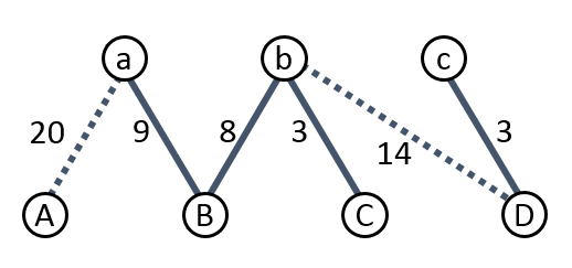
Consider the example in Figure 1(a), where elements are the edges in a graph and the feasibility constraint is the graphical matroid; that is, a set is feasible if it contains no cycles. Each edge is labeled with a value, and is being bid on by a different agent. The optimal outcome is $\{ab,ad,cd\}$, but the bid profile (where dashed lines get bid $0$) results in outcome $\{ac,bc,bd\}$. If the agent bidding on edge $ab$ raised his bid to half of its value, $3$, he would lose this bid; to which equilibrium payment should this loss be charged? A first instinct would be to charge against edge $ad$, since that edge sets the critical threshold for whether a bid on $ab$ would win. However, such a charging scheme would also charge losing bids for edges $ad$ and $cd$ to edge $ac$ as well, leading to poor smoothness bounds. To avoid such collisions, one must take a more global view, taking into account all deviations by all players. In this example, one could charge $ab$ to $ac$, $cd$ to $bd$, and $ad$ to $bc$. To build such a global charging method for general matroids, we use the Rota Exchange property of matroids, which guarantees the existence of an appropriate mapping on which to build a charging scheme.

Our main result is that any greedy mechanism that allocates resources subject to a matroid constraint has price of anarchy at most $3$ via a smoothness argument.

Roughly speaking, a mechanism is smooth if, for every valuation profile $v$, there is an action profile $a^{*}$ such that, for all bid profiles $b$, the sum of all agent payments (under $b$) plus the sum of agent utilities (under unilateral deviations from $b$ to $a^{*}$) is at least a constant factor of the optimal social welfare. To generalize previous smoothness arguments to arbitrary matroid environments, we must find a general method to charge losing bids (under deviation $a^{*}$) to agent payments (under $b$), as described above. We make use of the well-known Rota exchange property of matroids to build the necessary mappings. Mapping in hand, we employ a method of declared-welfare maximization recently developed in [1], paired with the composition framework of [19], to establish the claimed smoothness condition.

We next show that our result can be extended to handle polymatroid constraints. A formal definition of polymatroids appears in Section 3.1. Roughly speaking, a polymatroid allows fractional allocations of goods, subject to submodular constraints on the total allocated quantities of different subsets of goods. We actually provide two different forms of this extension. First, if each agent’s value for a good is linear in the amount of the good she receives, then we consider a greedy mechanism that asks agents to report their per-unit value of each good, then allocates the goods greedily. Second, we consider more general valuations that can be arbitrary submodular functions over the space of feasible allocations; in particular, they needn’t be linear for a single good. For this setting, we modify our mechanism to extend the bidding language slightly: it elicits from each agent a bid on each element of the ground set, where the bid includes a declared value per unit of the element, plus a maximum amount of the element that the agent is willing to accept. One can then consider the greedy allocation rule, which maximizes resources greedily subject to the polymatroid contraint, up to the declared caps. For both extensions, our analysis applies and we show that the greedy mechanism has a price of anarchy of at most $3$.

Our main theorem and extensions can be applied to a variety of auction settings, such as sponsored search auctions and combinatorial auctions. We discuss these applications in Section 4.

We then turn to matching constraints, where the elements for sale are edges in a bipartite graph and an allocation is feasible only if no two allocated edges are coincident. This is a special case of the intersection of two matroids. For this case we again show a constant price of anarchy via smoothness analysis, though this proof is more technically involved and we obtain a bound of $8$.²² 2 The technical difficulties we encounter bear some similarities to the independent work of Kesselheim et al. [9] who consider an auction setting that involves matroid constraints. They consider a greedy mechanism on the intersection of a “unit”-partition matroid and a separate matroid constraint for each player. This result is incomparable to ours, as we provide bounds for greedy algorithms on the intersection of two “unit”-partition matroids, i.e. matchings.

We conjecture that our results extend to the intersection of two arbitrary matroids, and perhaps even to the intersection of $k$ matroids (with a price of anarchy bound of $O(k)$). As progress toward understanding matroid intersections, we show that if the feasibility constraint is the intersection of $k$ matroids and the optimal allocation rule is used on the bids (rather than the greedy rule), then the price of anarchy is indeed $O(k)$. We emphasize here that this analysis is very different from that of different “optimal” allocation methods, such as the VCG mechanism. In particular, the allocation rule is being applied to a restricted bidding space, where agents must place separate bids on each item; the allocation returned is the optimal allocation for the bids, which necessarily describe only additive valuations.

Our results are similar in spirit to Borodin and Lucier [12], who also consider the price of anarchy of greedy mechanisms. They show that for a class of combinatorial auction problems, any $c$-approximate greedy algorithm has price of anarchy $O(c)$ when paired with a first-price payment rule. Our results are incomparable to theirs: they do not impose requirements on the feasibility constraints or the agents’ valuation classes, but they allow only greedy algorithms in which agents bid directly on their outcomes (e.g., a package of items in a combinatorial auction). Since our analysis doesn’t impose this last requirement, it applies to a wider array of greedy mechanisms, such as combinatorial auctions that allocate individual items or generalized sponsored search auctions that don’t require customers to bid directly on slots.

Babaioff, Lucier, Nisan, and Paes Leme [1] give a general price of anarchy analysis for “declared welfare maximizing” mechanisms, which collect bids (from a potentially limited bidding space) and then allocate optimally with respect to the bids. Our greedy mechanism for matroids is a declared welfare maximizer, but our analysis applies to a more general space of feasibility conditions; the analysis of [1] is specific to combinatorial auction constraints. That said, portions of our proofs apply techniques in a spirit similar to [1].

Bikhchandani et al. [3] design an ascending-price Vickrey-style auction for selling elements of a matroid. Their setting is identical to our own, except that it is assumed that agent values are additive over the elements they receive. They show that their mechanism is welfare-optimal and has a variety of desireable incentive properties. Our work extends their setting to the case of more general valuations, where greedy allocation rules are not necessarily incentive compatible.

We will denote with $SW:\mathcal{A}\times\mathcal{V}\rightarrow\mathbb{R}_{+}$, the social welfare produced by the mechanism under some action profile: $SW^{\mathcal{M}}(a;v)=\sum_{i\in[n]}\mathbb{E}_{X_{i}(a)}[v_{i}\left(X_{i}(a)\right)].$ For any valuation profile $v\in\mathcal{V}$ we will denote with $x^{*}(v)$ the optimal allocation, i.e. the allocation that maximizes welfare over all feasible allocations $x\in\mathcal{X}$ and we will denote with $\text{{Opt}}(v)=\sum_{i\in[n]}v_{i}(x_{i}^{*}(v))$.

We refer the reader to [19] for properties of smooth mechanisms. Roughly if a mechanism is $(\lambda,\mu)$-smooth, then every equilibrium has social welfare at least $\frac{\lambda}{\max\{1,\mu\}}$ of the optimal (i.e. the price of anarchy (PoA) is at most $\frac{\max\{1,\mu\}}{\lambda}$) and this extends to no-regret learning outcomes, incomplete information, simultaneous and sequentially occurring mechanisms and budget constraints.

Consider the following instantiation of the mechanism design setting: the allocation space $\mathcal{X}_{i}$ of each player $i$ consists of the power set of a finite set of elements $\mathcal{E}_{i}$ which we will refer to as the ground elements of player $i$. Hence, each bidder $i$’s valuation is a set function $v_{i}:2^{\mathcal{E}_{i}}\rightarrow\mathbb{R}_{+}$ which maps an allocation $S_{i}\subseteq\mathcal{E}_{i}$ to a value $v_{i}(S_{i})$. We will be primarily interested in the case where this function is XOS, i.e. can be expressed as a maximum over a set of additive valuations (see Lehmann et al. [11]), which is a superset of submodular valuations.

We denote with $\mathcal{E}=\mathcal{E}_{1}\cup\ldots\cup\mathcal{E}_{n}$ the set of all ground elements. The outcome of the mechanism is a subset $S\subseteq\mathcal{E}$ of this ground set and thereby the allocation of each player is $S_{i}=S\cup\mathcal{E}_{i}$. We assume that there is some feasibility constraint $F\subseteq 2^{\mathcal{E}}$ defined on $\mathcal{E}$, which defines which subsets $S\subseteq\mathcal{E}$ are feasible. The outcome of the mechanism is restricted to fall within $F$.

We consider the following mechanism: from each player $i$, the auctioneer solicits bids $b_{t}$ for each $t\in\mathcal{E}_{i}$, i.e. $\mathcal{A}_{i}=\mathbb{R}_{+}^{|\mathcal{E}_{i}|}$. We will denote with $a_{i}=(b_{t})_{t\in\mathcal{E}_{i}}$ an action of player $i$ and with $b=(b_{t})_{t\in\mathcal{E}}$ a bid profile on all elements. The auctioneer runs the greedy algorithm on the reported bid profile to decide which elements of $\mathcal{E}$ are to be picked, i.e. elements are considered in decreasing ordered of bids and each element is added to the outcome as long as it is feasible. Each player is asked to pay his bid for each of his elements in his allocation.

Another application of our setting is that of the simultaneous first price item-bidding auction. The simultaneous item bidding auction among $m$ items can be seen as matroid mechanism on a matroid of $n\cdot m$ elements, where each element corresponds to a (player, item) pair. Each player controls the $m$ elements in which he appears, one for each of the items. The feasibility constraint is that, for every item, only one of the elements containing that item can be in the outcome set, which is a matroid feasibility constraint. Note that the simultaneous first price item-bidding mechanism corresponds to the greedy first price mechanism on this matroid setting.

Our polymatroid result finds interesting application in the case of ad auctions. By Goel et al [7] the following setting can be represented as a polymatroid: there are multiple keywords and each keyword $j$ has $k$ slots available. Each slot $(j,k)$ is associated with a number of clicks $a_{j,k}$. A set of players is competing for the clicks. Each player has a per-click value $v_{i}$ and his value is $v_{i}\cdot x_{i}$, where $x_{i}$ is the number of clicks he got, i.e. if $k(i,j)$ is the position he won at keyword $j$, then $x_{i}=\sum_{j}k_{j,k(i,j)}$. The feasibility constraints in the above setting can be expressed as a polymatroid and therefore the greedy polymatroid mechanism yields a smooth mechanism. Note that the greedy polymatroid mechanism in this setting is to run independent Generalized First Price auctions for each keyword. In fact, our mechanism can handle the case where players have different valuations for different keywords, i.e. $\sum_{j}v_{ij}a_{j,k(i,j)}$. In this case, each keyword is a different coordinate of the polymatroid. The mechanism again corresponds to running a Generalized First Price auction, but now the players can submit a bid $b_{ij}$ for each keyword $j$.

Our polymatroid mechanism with capacities can also have applications if the valuations of the players are submodular over the allocated clicks from each keyword. However, the mechanism would not correspond to running GFP on each keyword. Instead, the mechanism would asks also for capacities of the players and then randomize over the allocation of positions so as in expectation a player is never allocated more than his declared click capacity.

As an illustration of the power of the polymatroid formulation, we revisit a model of sponsored search ad auctions with externalities studied by Roughgarden and Tardos [16]. Like the Ad Auction setting above, there are $k$ slots; for simplicity assume there is only one keyword. Each advertiser has a per-click value $v_{i}$, but also a click probability $p_{i}$ and a continuation probability $q_{i}$. Rather than presuming that each slot has a click probability, these probabilities arise as follows: given an assignment of ads to slots, a user will begin scanning the list of ads from slot $1$ to slot $k$. Upon encountering an ad $i$, say in slot $j$, it will click the ad with probability $p_{i}$. Also, with probability $q_{i}$ the user will continue scanning to the next slot; otherwise, with probability $1-q_{i}$ the user will terminate and not view any subsequent ads. Thus, if we write $\alpha(j)$ for the ad assigned to slot $j$, then the total value of an ad $i$ assigned to slot $\ell$ is $v_{i}p_{i}\prod_{j<\ell}q_{\alpha(j)}$.

In [16] it is shown that an auction that assigns ads to slots greedily by $\frac{v_{i}p_{i}}{1-q_{i}}$ and charges threshold payments has a price of anarchy of at most 4. We will describe how to interpret this setting as a polymatroid auction, and our results will then imply a price of anarchy of $3$ for a first price variant. Our result price of anarchy of $3$ for polymatroid auctions, though phrased for first price payments, can also be easily adapted to give a price of anarchy of at most $6$ for any second price variant, assuming players do not bid above their valuation.³³ 3 A fairly standard, in the literature, modification in the proof of our main theorem to show that the auction is weakly $(1/3,1)$-smooth as defined in [19], which implies a bound of $6$ on the price of anarchy Thus our polymatroid result directly implies a constant approximation for the auction analysed in [16].

Denote with $x_{i}$ the probability that ad $i$ is the last ad scanned. Then advertiser $i$ obtains expected value $\frac{v_{i}p_{i}}{1-q_{i}}\cdot x_{i}$. We can therefore write $V_{i}=\frac{v_{i}p_{i}}{1-q_{i}}$, and then view the auction as allocating the probabilities $x_{i}$ to bidders with modified values $V_{i}$. We now claim that the set allocation profiles $\mathbf{x}$ corresponding to valid assignments forms a polymatroid, with constraints given by $\sum_{t\in S}x_{t}\leq 1-\prod_{t\in S}q_{t}$. To see that the conditions are necessary, note that the probability that any ad in set $S$ is the last scanned is maximized when the ads in $S$ occupy the lowest-indexed slots, in which case the probability is precisely $1-\prod_{t\in S}q_{t}$. For sufficiency, note that any deterministic assignment certainly satisfies these constraints (consider all prefixes of the assignment), and hence any mixture of assignments would as well. Last observe that the function $f(S)=1-\prod_{t\in S}q_{t}$ is a monotone submodular function and therefore the polytope defined by these constraints is a polymatroid.

Since the setting can be framed as a polymatroid auction with values given by $\frac{v_{i}p_{i}}{1-q_{i}}$, we can conclude that a greedy auction that allocates in order of $\frac{v_{i}p_{i}}{1-q_{i}}$ is $(\frac{1}{3},1)$-smooth.

References

- [1] Babaioff, M., Lucier, B., Nisan, N., and Paes Leme, R. 2014. On the efficiency of the walrasian mechanism. In Proceedings of the Fifteenth ACM Conference on Economics and Computation. EC ’14. ACM, New York, NY, USA, 783–800.
- [2] Babaioff, M., Nisan, N., and Pavlov, E. 2009. Mechanisms for a spatially distributed market. Games and Economic Behavior 66, 2, 660–684.
- [3] Bikhchandani, S., de Vries, S., Schummer, J., and Vohra, R. V. 2011. An ascending vickrey auction for selling bases of a matroid. Operations Research 59, 2, 400–413.
- [4] Caragiannis, I., Kaklamanis, C., Kanellopoulos, P., Kyropoulou, M., Lucier, B., Leme, R. P., and Éva Tardos. 2014. Bounding the inefficiency of outcomes in generalized second price auctions. Journal of Economic Theory 0, –.
- [5] Christodoulou, G., Kovács, A., and Schapira, M. 2008. Bayesian combinatorial auctions. In Proceedings of the 35th international colloquium on Automata, Languages and Programming, Part I. ICALP ’08. Springer-Verlag, Berlin, Heidelberg, 820–832.
- [6] Demange, G., Gale, D., and Sotomayor, M. 1986. Multi-item auctions. Journal of Political Economy 94, 4, pp. 863–872.
- [7] Goel, G., Mirrokni, V., and Paes Leme, R. 2012. Polyhedral clinching auctions and the adwords polytope. In Proceedings of the 44th symposium on Theory of Computing. STOC ’12. ACM, New York, NY, USA, 107–122.
- [8] Hassidim, A., Kaplan, H., Mansour, Y., and Nisan, N. 2011. Non-price equilibria in markets of discrete goods. In Proceedings of the 12th ACM conference on Electronic commerce. EC ’11. ACM, New York, NY, USA, 295–296.
- [9] Kesselheim, T., Kleinberg, R., and Tardos, E. 2014. Smooth online mechanisms: A game-theoretic problem in renewable energy markets.
- [10] Lee, J., Sviridenko, M., and Vondrák, J. 2010. Submodular maximization over multiple matroids via generalized exchange properties. Math. Oper. Res. 35, 4, 795–806.
- [11] Lehmann, B., Lehmann, D., and Nisan, N. 2001. Combinatorial auctions with decreasing marginal utilities. In Proceedings of the 3rd ACM conference on Electronic Commerce. EC ’01. ACM, New York, NY, USA, 18–28.
- [12] Lucier, B. and Borodin, A. 2010. Price of anarchy for greedy auctions. In Proceedings of the Twenty-First Annual ACM-SIAM Symposium on Discrete Algorithms. SODA ’10. Society for Industrial and Applied Mathematics, Philadelphia, PA, USA, 537–553.
- [13] Markakis, E. and Telelis, O. 2012. Uniform price auctions: Equilibria and efficiency. In Algorithmic Game Theory, M. Serna, Ed. Lecture Notes in Computer Science. Springer Berlin Heidelberg, 227–238.
- [14] Roth, A. E. 2005. Pairwise kidney exchange. Journal of Economic Theory.
- [15] Roughgarden, T. 2012. The price of anarchy in games of incomplete information. SIGecom Exch. 11, 1, 18–20.
- [16] Roughgarden, T. and Tardos, E. 2012. Do externalities degrade gsp’s efficiency? In Eighth Ad Auctions Workshop.
- [17] Schrijver, A. 2003. Combinatorial Optimization: Polyhedra and Efficiency. Matroids, trees, stable sets. Number v. 2 in Algorithms and Combinatorics. Springer.
- [18] Syrgkanis, V. 2012. Bayesian games and the smoothness framework. CoRR abs/1203.5155.
- [19] Syrgkanis, V. and Tardos, E. 2013. Composable and efficient mechanisms. In Proceedings of the Forty-fifth Annual ACM Symposium on Theory of Computing. STOC ’13. ACM, New York, NY, USA, 211–220.
Appendix A Omitted Proofs
A.1 Polymatroids
Proof of Theorem 3.9 : It is well-known (see e.g. Bikhchandani et al. [3] or Schrijver [17]) that for a sufficiently small discretization of the allocation space in units, if we consider the extended ground set where each element , is duplicated times, then the feasibility constraint implied by the polymatroid on these extended element set is a matroid. Moreover, if we denote with the -th copy of element , then if we assign a weight of to each element , then as the discretization goes to zero, the greedy algorithm on the matroid corresponds to the greedy algorithm on the polymatroid. Subsequently the payment of the polymatroid mechanism coincides with the payment of the extended matroid mechanism, when run on bids for each copy of . Last if we denote with , then the value of a player for an allocation of discretized units, corresponds to the value of a player in the discretized matroid that has value for each copy of element .
Thus we can view the polymatroid mechanism as the limit of a matroid mechanism where the players are restricted to submit the same bid on all copies of the same element. If we show smoothness of this restricted bid mechanism, then the smoothness of the polymatroid mechanism will follow by taking the limit of the discretization to zero.
In order to show smoothness, the only thing we need to observe is that the deviations used in the smoothness proof of the matroid mechanism (Lemma 3.7) are simply scaled versions of the valuation of a player. Thus it is easy to see, that if such scaled versions are allowed in the restricted bid space, then the same proof shows smoothness of the matroid mechanism under the restricted bid space. This is formalized in the following observation.
Observation A.21
Suppose that a mechanism is -smooth. Consider the mechanism , which is identical to , with the exception that the action space of each player is restricted to some subset . If every action in the support of the deviations used to show smoothness of , fall into action space , then is also -smooth.
Since we assumed that the value of a player is additive and homogeneous, observe that the weight of a player for each element of the discretized matroid is identical for all copies of element . Thus the smoothness deviations of Lemma 3.7 would correspond to bidding for each element of , which is an action that belongs to the restricted strategy space. Thus the matroid mechanism is smooth even under this restricted space, as long as the value of a player for all copies of an element is identical. Hence, the theorem follows. ∎
Proof of Corollary 3.10 : We first recall the submodular valuations setting. Suppose that each player’s value is a monotone submodular function on the euclidean lattice defined on . Then from [19], we know that it can be expressed as: , with being an increasing concave function. Since, it is easy to see that every increasing concave function can be expressed as the maximum of functions that are linear up to a point and then constant: i.e. , we can conclude that any submodular valuation can be written as . for some index set . Thus in order to prove smoothness of the polymatroid mechanism, by Lemma 3.6 it suffices to show smoothness for the following much simpler class of valuations: .
However, we readily observe that if we consider an arbitrarily small discretization of the polymatroid then the valuations of the players for the copies of an element , will not be identical. Instead, if we consider some arbitrary order of the copies, then the player will have a value of for the first copies and zero value for subsequent copies. Thus to render the polymatroid mechanism smooth, we need to allow for the player to express such valuations for the copies of the same element. To achieve this we introduce the modification of the polymatroid mechanism under which the player can also submit allocation capacities for each good.
If we consider an arbitrarily small discretization of the polymatroid, then the player can submit a valuation that is , for the first copies of element and zero for the remaining, by simply submitting a weight of and a capacity of , to the polymatroid mechanism with capacities. ∎