SPIN–ORBIT ANGLES OF KEPLER-13A${\rm b}$ AND HAT-P-7${\rm b}$
FROM GRAVITY-DARKENED TRANSIT LIGHT CURVESNote: Accepted to ApJ

We basically follow Barnes [3] in modeling the gravity-darkened transit light curve. The model includes the following 14 parameters, which are listed as “fitting parameters” in Tables 1 and 3:

1. 1.

   mean stellar density, $\rho_{\star}=3M_{\star}/4\pi R_{\star}^{3}$, which corresponds to the semi-major axis scaled by the stellar equatorial radius, $a/R_{\star}$¹¹ 1 In this paper, $R_{\star}$ denotes the equatorial radius of the star.

2. 2.

   limb-darkening coefficient for the quadratic law, $c_{1}=u_{1}+u_{2}$,

3. 3.

   limb-darkening coefficient for the quadratic law, $c_{2}=u_{1}-u_{2}$,

4. 4.

   time of the inferior conjunction, $t_{c}$,

5. 5.

   orbital period, $P$,

6. 6.

   cosine of orbital inclination, $\cos i_{\rm orb}$,

7. 7.

   planetary radius normalized to the stellar equatorial radius, $R_{\rm p}/R_{\star}$

8. 8.

   normalization of the out-of-transit flux, $F_{0}$

9. 9.

   stellar mass, $M_{\star}$,

10. 10.

    stellar rotation frequency, $f_{\rm rot}$

11. 11.

    stellar effective temperature at the pole, $T_{\star,\rm pole}$

12. 12.

    gravity-darkening exponent, $\beta$,

13. 13.

    stellar inclination, $i_{\star}$

14. 14.

    sky-projected spin–orbit angle, $\lambda$.

The first eight parameters are common with the light-curve model without gravity darkening. We assume circular orbits for the two targets because the orbital eccentricities are constrained to be very small, if any, from the occultation light curves [33, 7].

In the gravity-darkened model by Barnes [3], the shape of the star is approximated by the spheroid with the oblateness $\gamma=\Omega_{\star}^{2}R_{\star}^{3}/2GM_{\star}=3\pi f_{\rm rot}^{2}/2G\rho_{\star}$. The surface brightness at each point is modeled as the blackbody emission of the temperature $T_{\star}=T_{\star,\rm pole}\left(g_{\rm eff}/g_{\rm eff,pole}\right)^{\beta},$ where $g_{\rm eff}/g_{\rm eff,pole}$ is the effective surface gravity normalized by its value at the stellar pole. The surface gravity at point $\bm{r}$ on the stellar surface is calculated by $\bm{g}_{\rm eff}=-GM_{\star}r^{-2}\bm{\hat{r}}+4\pi^{2}f_{\rm rot}^{2}r_{\perp}\bm{\hat{r}_{\perp}}.$ Here $r$ and $\bm{\hat{r}}$ are the norm and unit vector of the radius vector $\bm{r}$, respectively. Similarly, $r_{\perp}$ and $\bm{\hat{r}_{\perp}}$ are those of $\bm{r_{\perp}}$, the projection of $\bm{r}$ onto the stellar equatorial plane. The Planck function $B_{\lambda}(T_{\star})$ at each point is convolved with the “high-resolution” Kepler response function²² 2 http://keplergo.arc.nasa.gov/CalibrationResponse.shtml using the table of the wavelength- and temperature-dependent factor calculated prior to the fitting. The convolved flux is then multiplied by the limb-darkening function

with $\mu$ being the cosine of the angle between $-\bm{g}_{\rm eff}$ and our line of sight,³³ 3 Although this vector $-\bm{g}_{\rm eff}$ is not exactly parallel to the surface normal of the spheroid we assume, the difference is $\mathcal{O}(\gamma^{2})$ and thus negligible. and integrated over the visible surface of the star to give the total flux. We fix $T_{\star,\rm pole}$ at the observed effective temperature assuming that the difference between $T_{\star,\rm pole}$ and the disk-integrated effective temperature is small. Note that the gravity-darkened transit light curve gives $\rho_{\star}$ alone and can not constrain $M_{\star}$ and $R_{\star}$ separately, as is the case for the transit without gravity darkening.

The configuration of the planetary orbit and stellar spin is specified by three angles, $i_{\rm orb}$, $i_{\star}$, and $\lambda$, which are defined in Figure 1 [7, see also figure 1 of]. The orbital and stellar inclinations, $i_{\rm orb}$ and $i_{\star}$, are measured from the line of sight and defined to be in the range $[0,\pi]$. The sky-projected spin–orbit angle, $\lambda$, is the angle between the sky-projected stellar spin and planetary orbital axes. It is measured from the former to the latter counterclockwise in the sky plane, and is in the range $[0,2\pi]$. With these definitions, the true spin–orbit angle, or the stellar obliquity, $\psi$, is given by equation 1 of Benomar et al. [7]:

Throughout the paper, we restrict $i_{\star}$ to be in the range $[0,\pi/2]$ making use of the intrinsic symmetry with respect to the sky plane. We do not lose any physical information of the system with this choice because any of the relative star–planet configurations with $i_{\star}$ in $[\pi/2,\pi]$ is the same as one of those with $i_{\star}$ in $[0,\pi/2]$. In other words, the configurations $(i_{\star},i_{\rm orb},\lambda)$ and $(\pi-i_{\star},\pi-i_{\rm orb},-\lambda)$ are equivalent. This transformation corresponds to looking at the system from the other side of the plane of the sky.

In the following, we also adopt the constraint on the stellar line-of-sight rotational velocity $v\sin i_{\star}$ from spectroscopy, which is related to the above model parameters by

This, in principle, allows us to break the degeneracy between $M_{\star}$ and $R_{\star}$, enabling the determination of the absolute dimension of the system. Nevertheless, the constraint on $M_{\star}$ is usually weak as discussed in B11, and so we fix $M_{\star}$ at the observed value.

We detrend and normalize the transit light curves of each target along with the consistent determination of the transit times and transit parameters. We first normalize the light curve of each quarter using its median, and then iterate the following two steps until the resulting transit times $t_{c}$ and transit parameters converge (typically 10–20 times):

1. 1.

   Light curve around each transit ($\pm 0.2\,\mathrm{days}$ for Kepler-13A and $\pm 0.15\,\mathrm{days}$ for HAT-P-7) is modeled as the product of a quadratic polynomial⁴⁴ 4 Use of the quadratic polynomial helps the better removal of flux variation not due to the transit, i.e., planetary light, ellipsoidal variation, and Doppler beaming. $a_{0}+a_{1}(t-t_{c})+a_{2}(t-t_{c})^{2}$ ($t$: time) and the analytic transit light-curve model by Mandel & Agol [25]. We use the Levenberg-Markwardt (LM) method [26] to fit $a_{0}$, $a_{1}$, $a_{2}$, and $t_{c}$ iteratively removing $5\sigma$ outliers, while the other parameters are fixed. The filtered data are then divided by the best-fit polynomial to give a normalized and detrended transit light curve. We discard the transits with data gaps of more than $50\%$.

2. 2.

   Using the set of $t_{c}$ obtained in the first step, we calculate the mean orbital period $P$ and transit epoch $t_{0}$ by linear fit and use them to phase-fold the normalized and detrended transits. The phase-folded light curve is averaged into one-minute bin and then fitted with the Mandel & Agol [25] model using an LM algorithm. We fit $c_{1}$, $c_{2}$, $\rho_{\star}$, $\cos i_{\rm orb}$, $R_{\rm p}/R_{\star}$, and $F_{0}$, whose best-fit values are used in the step 1 of the next iteration. In this step, the orbital period $P$ is fixed to be the value obtained from the linear fit and the central time of the phase-folded transit is fixed to be zero.

In the following analysis, we use the one-minute binned, phase-folded light curve obtained in the second step of the final iteration. For each bin, the flux value is given by its mean and the error is estimated as the standard deviation within the bin divided by the square root of the number of data points.

In fitting the observed light curves, the likelihood $\mathcal{L}$ of the model is computed by $\mathcal{L}\propto\exp(-\chi^{2}/2)$, where

In the first term, $f_{i}$, $f_{\mathrm{model},i}$, and $\sigma_{i}$ are the observed value, modeled value, and error of the $i$th flux data. The second term is introduced to take into account the constraints from other observations on some (functions) of the model parameters ${p_{j}}$. In the following analysis, $p$ is read to be $v\sin i_{\star}$ and, in some cases, $\lambda$.⁵⁵ 5 Only in Section IV.1, $\rho_{\star}$, $c_{1}$, $c_{2}$, $R_{\rm p}/R_{\star}$, and $f_{\rm rot}$ are also included. For each $p_{j}$, we assume a Gaussian constraint of the form $p_{j}\pm\delta p_{j}$ and the value obtained from the model is denoted by $p_{\mathrm{model},j}$.

The maximum likelihood solution is found by minimizing Equation (4) with the LM method using the cmpfit package [26]. Since the complex dependence of $\chi^{2}$ on $i_{\star}$ and $\lambda$ is expected, we repeat the fitting procedure from the initial $i_{\star}$ in $[0,90^{\circ}]$ and $\lambda$ in $[-180^{\circ},180^{\circ}]$ at $10^{\circ}$ intervals. Initial values of the other parameters are chosen close to the best-fit values obtained from the model without gravity darkening. We also try both positive and negative $\cos i_{\rm orb}$ as an initial value to search the whole domain of $i_{\rm orb}$, which is now $[0^{\circ},180^{\circ}]$.

In this subsection, we analyze the short-cadence (SC), Pre-search Data Conditioned Simple Aperture Photometry (PDCSAP) fluxes from Q2, 3, and 7–17. Given the clear transit duration variation (TDV) reported by Szabó et al. [37] and Szabó et al. [38], we separately analyze the transits from each quarter, rather than folding all the available data. Since we do not detect significant temporal variations in the parameters other than $\cos i_{\rm orb}$ (see Section IV), we report the mean and standard deviation of the best-fit values from the above 13 quarters for each parameter.

First, we use the same stellar parameters as in B11 and obtain the results in the second column of Table 1. Namely, we subtract a constant value $F_{\rm c}=0.45$ from the normalized flux to remove the flux contamination from the companion star, and impose the constraint $v\sin i_{\star}=65\pm 10\,\mathrm{km\,s^{-1}}$ based on Szabó et al. [39]. We fix $M_{\star}=1.83M_{\odot}$ and $T_{\star,\rm pole}=8848\,\mathrm{K}$ from Borucki et al. [8], and $c_{2}=0$. In Figure 2, the best-fit model is overplotted with the data for Q2, which is to be compared with figure 2 of B11.

Basically, we find a very good agreement with the result by B11 using about $12$ times more data. Although the values of $\cos i_{\rm orb}$, $i_{\star}$, and $\lambda$ we report here appear different from those in B11, that is simply because we choose $i_{\star}$ to be in the range $[0,\pi/2]$. This is physically the same configuration as theirs and corresponds to the top-left situation in figure 3 of B11. That is, $\lambda$ in our solutions with $\cos i_{\rm orb}<0$ should be read as $-\lambda$ in the conventional definition, because $\lambda$ is usually defined for the orbit with $\cos i_{\rm orb}>0$ (see also the discussion after Equation 2).

In addition to the solution in Table 1, we also find a retrograde solution with $\lambda>90^{\circ}$ as noted in B11. Here we do not discuss this solution, however, because the Doppler tomography observation has already excluded the retrograde orbit with high significance [20].

Although we find consistent values of $\lambda$ and $i_{\star}$ as obtained by B11, those of $\lambda$ significantly differ from $\lambda=58.\negthickspace^{\circ}6\pm 2.\negthickspace^{\circ}0$, the value obtained from the Doppler tomography [20]. Motivated by this discrepancy, we investigate the possible origins of systematics in the spin–orbit angle determination with gravity darkening in this subsection.

First, we examine the systematics due to the choice of $M_{\star}$, $v\sin i_{\star}$, $T_{\star,\rm pole}$, and $F_{\rm c}$, which are the stellar properties not derived from the light curve modeling.⁶⁶ 6 We do not examine the dependence on $\beta$ here because B11 have already shown that a different choice of $\beta=0.19$, suggested by the interferometric observation of Altair [28], does not change the result significantly. We perform the same analysis as in Section III.1, but adopting the following parameters from the most recent photometric and spectroscopic study by Shporer et al. [33, hereafter S14]: $v\sin i_{\star}=78\pm 15\,\mathrm{km\,s^{-1}}$, $M_{\star}=1.72M_{\odot}$, $T_{\star,\rm pole}=7650\,\mathrm{K}$, and $F_{\rm c}=0.47726$. The corresponding results are shown in the third column of Table 1. We find that $i_{\star}$ and $\lambda$ can differ by as large as $10^{\circ}$ due to the choice of the above parameters, but the difference is not so large as to explain the disagreement with the Doppler tomography. The main difference from the B11 case with this new set of parameters is the different constraint on $f_{\rm rot}\sin i_{\star}$, which is proportional to the combination $(\rho_{\star}/M_{\star})^{1/3}v\sin i_{\star}$ (c.f., Equation 3). With smaller $M_{\star}$ and larger $v\sin i_{\star}$, the stellar rotation rate slightly higher than the B11 case is favored. We find that the difference in $T_{\star,\rm pole}$ is less important compared to the above effect. We also find that larger $F_{\rm c}$ yields larger $R_{\rm p}/R_{\star}$, which makes the impact parameter or $|\cos i_{\rm orb}|$ smaller to give the same ingress/egress duration.

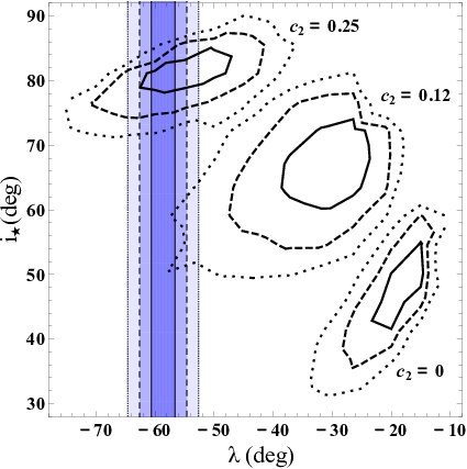
Next, we allow $c_{2}=u_{1}-u_{2}$ to be free, and find that the resulting spin–orbit angle is very sensitive to this parameter. When $c_{2}$ is floated, the constraints on $i_{\star}$ and $\lambda$ become much weaker than the $c_{2}=0$ case, as shown in the fourth and fifth columns of Table 1. The strong dependence on $c_{2}$ is illustrated in Figure 3, which shows that $\lambda$ and $i_{\star}$ vary by several tens of degrees depending on $c_{2}$. In fact, the result indicates that the gravity-darkened light curve is actually compatible with the Doppler tomography solution if we choose $c_{2}\sim 0.25$; such a solution will be discussed in Section III.3.

In Section III.2, we found that the gravity-darkened light curve is compatible with the value of $\lambda$ estimated from the Doppler tomography if $c_{2}\sim 0.25$. Thus we repeat the analysis treating $c_{2}$ as a free parameter for both stellar parameters by B11 and S14, but this time imposing additional constraint $\lambda=58.\negthickspace^{\circ}6\pm 2.\negthickspace^{\circ}0$ from the Doppler tomography. The results are summarized in the last two columns in Table 1. The resulting value of $i_{\star}=81^{\circ}\pm 5^{\circ}$ indicates that the star is close to equator-on, and $\psi=60^{\circ}\pm 2^{\circ}$ is slightly larger than the previous estimate. In terms of $\chi^{2}_{\rm min}$, these solutions equally well reproduce the transit anomaly as the solutions discussed so far, and still they are consistent with the Doppler tomography result. Moreover, we obtain a slightly longer $P_{\rm rot}$, which better agrees with $P_{\rm rot}=25.43\pm 0.05\,\mathrm{h}$ estimated by Szabó et al. [37] and Szabó et al. [38] than the solution with the gravity darkening alone. For these reasons, the joint solution is most favored from the current observations.

We note, however, that the likelihood for the joint solution is not so high as to statistically justify the introduction of the additional free parameter $c_{2}$. Furthermore, the plausibility of the value of $c_{2}$ in our joint solution is theoretically unclear. We obtain the theoretical values of $c_{1,\rm th}\simeq 0.6$ and $c_{2,\rm th}\simeq 0.0$ from the table of Sing [34] if we adopt the effective temperature and surface gravity by S14. Hence the value of $c_{2}$ from our joint solution is discrepant from $c_{2,\rm th}$; they could even have opposite signs depending on the stellar parameters. Nevertheless, it is also true that theoretical values often disagree with the observed ones [35, e.g.,]; in fact, $c_{1}$ in the light-curve solution with $c_{2}=0$ is also different from $c_{1,\rm th}$. Therefore, we do not consider the possible deviations from the theoretical values crucial, and regard it as an open question.⁷⁷ 7 For reference, we find $c_{2}=0.1\mathchar 450.2$ if we adopt the model without gravity darkening [25], which suggests that the choice of $c_{2}=0$ is not indispensable. An alternative approach to independently assess the validity of our solution is discussed in the next section.

To examine the temporal variations in $\cos i_{\rm orb}$, $i_{\star}$, and $\lambda$, we fit individual transit light curves, rather than the phase-folded ones, for these parameters. We use the same two models (“light-curve solution” with $c_{2}=0$ and “joint solution” with $c_{2}$ fitted) as discussed in Section III. In order not to underestimate the errors in the three angles, we fit all the other model parameters, $\rho_{\star}$, $c_{1}$, $c_{2}$ (for the joint model), $t_{c}$, $R_{\rm p}/R_{\star}$, $f_{\rm rot}$, and $F_{0}$ as well, which should not vary temporally in our model. Using the best values in Table 1, we impose the constraints on these parameters except for $t_{c}$ and $F_{0}$, through the second term of Equation (4). In fitting much noisier individual transits, this prescription assures that the parameters converge to the values consistent with those from the phase-folded light curves, while preserving their differences from transit to transit. We also discard the transits for which fit does not converge due to the data gaps and/or flare-like brightening features sometimes found in the light curves. The resulting sequences of the transit parameters are plotted in Figure 4.

As mentioned above, we again find the clear linear trend in $\cos i_{\rm orb}$ from individual transits. We fit the linear model to the time series of $\cos i_{\rm orb}$ using a Markov Chain Monte Carlo (MCMC) algorithm and obtain the rates of change in the upper part of Table 2. Here we only report the slopes for absolute values of $\cos i_{\rm orb}$ because its actual sign depends on the sign of $\cos i_{\star}$, which can never be determined with the current observations (we arbitrarily choose $\cos i_{\star}>0$ in this paper, as discussed after Equation 2). Comparing the light-curve solution and joint solution, we find that the rate of $|\cos i_{\rm orb}|$ change is insensitive to $\lambda$ or $c_{2}$ because $|\cos i_{\rm orb}|$ is mainly determined from the transit duration. With $a/R_{\star}$ calculated from $\rho_{\star}$, our value for $\mathrm{d}|\cos i_{\rm orb}|/\mathrm{d}t$ is found to be consistent with $\mathrm{d}b/\mathrm{d}t=(-4.4\pm 1.2)\times 10^{-5}\,\mathrm{day}^{-1}$ by Szabó et al. [37], but our constraint is several times better.

Figure 4 also shows the abrupt systematic changes in $R_{\rm p}/R_{\star}$. These changes occur exactly in phase with the border of different quarters indicated with different colors (black and gray). For this reason, they are unlikely to be of physical origin, but are probably due to the seasonal transit depth variations similar to those reported by Van Eylen et al. [40] for HAT-P-7. In addition, some of the parameters (most notably $\rho_{\star}$ and $f_{\rm rot}$) show the long-term modulation of the period $\sim 400\,\mathrm{days}$. Origins of these systematics are beyond the scope of this paper, and they are just treated as the additional scatter in the data.

Among the observed time series of transit parameters in Figure 4, those of $\cos i_{\rm orb}$, $\lambda$, and $i_{\star}$ are fitted using an MCMC algorithm to observationally constrain $J_{2}$ and $\mathbb{C}$. We utilize the same analytic precession model as in Barnes et al. [5], which constitutes an analytic solution of the secular equations of motion derived by Boué & Laskar [9]. In this model, the orbital and spin angular momenta precess around the total angular momentum at the same angular rate given by

where $\dot{\Omega}_{\rm p}$ is the precession rate of the orbital angular momentum around the stellar spin, and explicitly given by

with $J_{2}$ being the stellar quadrupole moment. In the Kepler-13A system, the spin angular momentum, $S$, is comparable to the orbital one, $L$, owing to the small semi-major axis and rapid stellar rotation. As a consequence, $\dot{\Omega}$ also depends on the ratio of the two,

where $\mathbb{C}$ is the moment of inertia coefficient of the host star. Thus, the independent model parameters are $\rho_{\star}$, $f_{\rm rot}$, $J_{2}$, $\mathbb{C}$, $P$, $M_{\rm p}/M_{\star}$, and three angles $\cos i_{\rm orb}$, $\lambda$, $i_{\star}$ at some epoch (here taken to be $\mathrm{BJD}=2454833+800$). We do not relate $J_{2}$ to the other parameters like the stellar oblateness as done in Barnes et al. [5].

To realistically evaluate the credible intervals of $J_{2}$ and $\mathbb{C}$ by marginalization, uncertainties in $\rho_{\star}$, $f_{\rm rot}$, $P$, and $M_{\rm p}/M_{\star}$ should also be taken into account. However, these parameters are not well determined from the data of $\cos i_{\rm orb}$, $\lambda$, and $i_{\star}$. Thus, they are floated with the following Gaussian priors. The first three are assigned the same central values and widths as in Table 1. For the mass ratio, we take the mean and standard deviation of the results reported by S14, Esteves et al. [14], and Faigler & Mazeh [16], which come from the amplitudes of the ellipsoidal variation and Doppler beaming. We also impose the Gaussian prior on $\mathbb{C}$ centered on $0.0776$ [37, the value for $n=3$ polytrope by] and with the width of $0.02$, which is chosen to enclose the solar value, $0.059$.

The constraints from the MCMC fit are summarized in the middle and bottom parts of Table 2 and the best-fit models are plotted with the solid lines in Figure 5. Basically, the precession model is compatible with the observations both for the light-curve solution and the joint solution. The value of $J_{2}$ and the corresponding precession period, however, are different by a factor of a few, in spite of the similar observed slopes in $\cos i_{\rm orb}$. While $J_{2}=(1.66\pm 0.08)\times 10^{-4}$ for the light-curve solution is consistent with the earlier estimate by Szabó et al. [37], $J_{2}=(2.1\pm 0.6)\times 10^{-4}$ from observed TDVs and $J_{2}=1.7\times 10^{-4}$ from the stellar model, the joint solution yields a smaller value, $J_{2}=(6.1\pm 0.3)\times 10^{-5}$.

The difference comes from the different three-dimensional architectures of the system described by the two solutions. Since all of $\cos i_{\rm orb}$, $\lambda$, and $i_{\star}$ are constrained from the gravity-darkened light curves, relative configuration of the stellar spin and orbital angular momenta are completely specified in three dimensions. This means that the phase of the precession during the Kepler mission, which corresponds to the left end in the right column of Figure 6, is observationally constrained; from the top panel, we find that $\cos i_{\rm orb}$ is closer to the bottom of the sine curve for the light-curve solution (blue dashed line), while that for the joint solution (red solid line) resides in the phase of a rapid increase. For this reason, a larger precession rate (i.e., shorter precession period) is required for the light-curve solution to match the observed change in $\cos i_{\rm orb}$. According to Equations (5) and (6), the larger precession rate can be achieved by increasing either $J_{2}$ or $L/S$. However, the larger precession rate also induces faster variations in $\lambda$ and $i_{\star}$, contradicting their almost constant observed values (middle and bottom panels in Figure 5). The only way to mitigate this conflict is to make $J_{2}$ larger (i.e., increase the precession rate) while keeping $L/S$ small, making it more difficult to move stellar spin axis. With Equation (7), this explains why $M_{\rm p}/M_{\star}$ is smaller and $\mathbb{C}$ is larger for the light-curve solution than for the joint solution in Table 2. Accordingly, the bottom panel of the right column in Figure 6 exhibits the smaller precession amplitude for $i_{\star}$ in the former solution (blue dashed line) than the latter (red solid line).

The approximately three times difference in the precession period would be apparent even on the short time scale (left column in Figure 6). As shown in the middle panel, as large as $\sim 10^{\circ}$ change in $\lambda$ is expected within the next $\sim 10\,\mathrm{yr}$ for the light-curve solution, which may well be detectable given the current precision of the spin–orbit angle measurement (nominally down to a few degrees). On the other hand, $\lambda$ for the joint solution is almost constant. From this point of view, the joint solution may slightly be favored even with the current data, because the nearly-constant values observed for $\lambda$ and $i_{\star}$ are more natural for the joint solution than for the light-curve one, for the reasons discussed in the previous paragraph. This indication also manifests itself in the fact that the resulting $M_{\rm p}/M_{\star}$ and $\mathbb{C}$ better agree with our prior knowledge in the joint solution.

The more decisive conclusion will be obtained with the future follow-up observations of $\lambda$ using Doppler tomography, as well as the transit duration observations to better constrain $\cos i_{\rm orb}$, and hence the precession rate. If our joint solution is correct, variations in $\lambda$ will not be detected in near future. On the other hand, if the light-curve solution is actually correct and $\lambda$ from the Doppler tomography is somehow systematically biased, $\lambda$ should change; this temporal variation would be observable with the Doppler tomography even if it were biased. Or, it may even turn out that the precession scenario is wrong. In any case, tracking the future evolution of the system configuration can be used for an independent test of our solution, not to mention for better constraining stellar internal structure via $J_{2}$ and $\mathbb{C}$, for which few observational constraints have been obtained.

If the observed anomaly is really due to gravity darkening, it should be persistent over all observation span. It is important to confirm the property because Morris et al. [29] only reported the bump before the mid-transit time. Thus, we divide the transits into four consecutive groups (Q0–4, 5–9, 10–13, 14–17), phase-fold and fit each of them with the model without gravity darkening separately, and examine the shapes of the residuals. Although fewer numbers of transits lead to noisier phase-folded light curves, ten-minute binned residuals in the left column of Figure 7 exhibit a similar feature (brightening before mid-transit and dimming after it) in every span of data.

Besides, Van Eylen et al. [40] reported seasonal variation in the transit depth depending on the quarter, which is reproduced in our analysis with Q0--17 data.¹⁰¹⁰ 10 We also reported a similar phenomenon in Kepler-13A; see Section IV.1 and Figure 4. To confirm that the anomaly is not an artifact related to this seasonal variation, we also perform a similar analysis as above but this time grouping the transits that have similar depths. As shown in the right column of Figure 7, we find that the same feature is apparent regardless of the season and the anomaly is not affected by the systematic depth variation. For this reason, along with its unconstrained origin, we do not try to make corrections for this systematic in the following analyses.

As in Section III, we consider both light-curve solution and joint solution that takes into account the constraints from other observations. First, the light-curve solution is obtained with $c_{2}$ fixed to be zero (Figure 8, second and third columns in Table 3). In this case, we find two solutions with different signs of $\cos i_{\rm orb}$, which are indistinguishable in terms of the minimum $\chi^{2}$.¹¹¹¹ 11 The existence of the two solutions in this case should be distinguished from the degeneracy intrinsic to the gravity-darkening method. For each of the two solution listed here, there additionally exists the model that yields exactly the same light curve, where $\cos i_{\rm orb}$ is replaced with $-\cos i_{\rm orb}$ and $\lambda$ with $\pi-\lambda$. These intrinsically-degenerate solutions are not discussed here because they are in any case rejected in the joint solution, where $\lambda$ is constrained by the prior. This is the same logic as used in the last paragraph of Section III.1. The values quoted in Table 3 are the median, 15.87, and 84.13 percentiles of the MCMC posteriors sampled with emcee [18].¹²¹² 12 We also applied the residual permutation method described in Winn et al. [44] for another estimate of the parameter uncertainties, and confirmed that they are not significantly affected by the correlated noise component. Our model reasonably reproduces the global feature of the anomaly (positive before the mid transit and negative after it), yielding $\Delta\chi^{2}\simeq 166$ for $\sim 420$ degrees of freedom. We compute the Bayesian information criterion (BIC) for the best-fit models with and without gravity darkening, and find $\Delta\mathrm{BIC}=129$, which formally indicates that the gravity-darkened model is strongly favored.

Our solution points to a nearly pole-on configuration with $i_{\star}\simeq 0^{\circ}$. This conclusion is consistent with the recent asteroseismic analyses by Benomar et al. [7] and Lund et al. [24], but the nominal constraint on $i_{\star}$ from the gravity-darkened model is much tighter. On the other hand, $\lambda$ is not constrained very well with the light curve asymmetry alone. The difficulty is inevitable in the pole-on configuration, where the brightness distribution on the stellar disk is almost axisymmetric even in the presence of gravity darkening. In such a case, $\psi$ is always close to $90^{\circ}$ regardless of $\lambda$.

One remaining issue regarding our solution is that the resulting rotation frequency may be too large. Given the age ($\simeq 2\,\mathrm{Gyr}$) and $B-V$ [24, $=0.495\pm 0.022$;] of the host star, the rotation frequency from the light-curve solution, $f_{\rm rot}=7.7\pm 0.2\,\mathrm{\mu Hz}$ (equivalent to $P_{\rm rot}\simeq 1.5\,\mathrm{days}$), is consistent with the gyrochronology relation by Meibom et al. [27]; see Section 6 of Lund et al. [24]. However, our value of $f_{\rm rot}$ is much larger than those from asteroseismology, $0.70_{-0.43}^{+1.02}\,\mathrm{\mu Hz}$ [7, $68\%$ credible interval by] and $<0.8748\,\mathrm{\mu Hz}$ [24, $1\sigma$ upper limit by]. In fact, the prior used in these analyses, $|f_{\rm rot}|<8\,\mathrm{\mu Hz}$, does not fully cover the range we investigate here with the gravity-darkened light curve. Still, the discrepancy is only weakly reduced even with the new analysis adopting the prior range extended up to $17\,\mathrm{\mu Hz}$, which yields $f_{\rm rot}=0.82_{-0.50}^{+2.02}\,\mathrm{\mu Hz}$ as the $68\%$ credible interval [7, by courtesy of Othman Benomar; see also].

To examine if the gravity-darkened model is compatible with the seismic analysis, we then search for a joint solution including the constraints both from the RM measurement and asteroseismology. From the RM effect, we incorporate the constraint $\lambda=172^{\circ}\pm 32^{\circ}$, which comes from the average and standard deviation of the analyses for the three different radial velocity data [7]. From asteroseismology, we adopt the above updated posterior for $f_{\rm rot}$ as the prior, and performed an MCMC sampling with emcee. To properly take into account the uncertainty from the limb-darkening profile, $c_{2}$ is also floated. The resulting credible intervals are summarized in the fourth and fifth columns in Table 3, and the model that maximizes the likelihood multiplied by the prior on $f_{\rm rot}$ is plotted with a dashed line in Figure 8. We again find two equally good solutions, both of which indicate nearly pole-on configurations with slightly prograde and retrograde orbits, $\psi=101^{\circ}\pm 2^{\circ}$ and $\psi=87^{\circ}\pm 2^{\circ}$. Although the resulting $f_{\rm rot}$ still prefers a higher rotation rate than that from asteroseismology, their difference is now mitigated to the $2\sigma$ level; we construct the probability distribution for $\Delta f_{\rm rot}$, $f_{\rm rot}$ from out joint analysis minus $f_{\rm rot}$ from asteroseismology, using their posteriors and find its $2\sigma$ credible region as $\Delta f_{\rm rot}=4.9_{-5.0}^{+4.0}\,\mu\mathrm{Hz}$. We argue that the level of discrepancy is acceptable, considering that the rotational mode splitting is not clearly detected in the power spectrum of HAT-P-7’s light curves.

Finally, it is also worth considering the case where $\beta\neq 0.25$, given the unconstrained nature of the gravity darkening in F dwarfs. Smaller values of $\beta\sim 0.08$ are usually expected for solar-like stars with convective envelopes [23, 10, e.g.,], while Espinosa Lara & Rieutord [11] and Espinosa Lara & Rieutord [12] argue that $\beta$ is close to $0.25$ in the limit of slow rotation under several assumptions. We repeat the above joint analysis floating $\beta$ with the prior uniform between $0$ and $0.3$, and obtain $\beta=0.26_{-0.05}^{+0.03}$ for both solutions in Table 3. On the one hand, the fact may support the claims by Espinosa Lara & Rieutord [11] and Espinosa Lara & Rieutord [12]; on the other hand, it may simply indicate some incompleteness in our gravity-darkening model, as also suggested by the tension in $f_{\rm rot}$ and the still correlated residuals before the mid transit (bottom panel of Figure 8). Indeed, if $\beta=0.08$ is adopted, we find that even higher rotation rate ($>10\,\mathrm{\mu Hz}$) is favored, making the discrepancy with asteroseismology more serious. Although the validity of $\beta$ we obtain is beyond the scope of this paper, we note that our conclusion for a pole-on orbit is robust against the adopted value of $\beta$; in both analyses where $\beta$ is fitted and $\beta$ is fixed to be $0.08$, the constraints on $\psi$ differ less than $1\sigma$ from the results in Table 3.

References

- [1] Ahlers, J. P., Seubert, S. A., & Barnes, J. W. 2014, ApJ, 786, 131
- [2] Albrecht, S., et al. 2012, ApJ, 757, 18
- [3] Barnes, J. W. 2009, ApJ, 705, 683
- [4] Barnes, J. W., Linscott, E., & Shporer, A. 2011, ApJS, 197, 10
- [5] Barnes, J. W., van Eyken, J. C., Jackson, B. K., Ciardi, D. R., & Fortney, J. J. 2013, ApJ, 774, 53
- [6] Bate, M. R., Lodato, G., & Pringle, J. E. 2010, MNRAS, 401, 1505
- [7] Benomar, O., Masuda, K., Shibahashi, H., & Suto, Y. 2014, PASJ, 66, 94
- [8] Borucki, W. J., et al. 2011, ApJ, 736, 19
- [9] Boué, G., & Laskar, J. 2009, Icarus, 201, 750
- [10] Claret, A. 1998, A&AS, 131, 395
- [11] Espinosa Lara, F., & Rieutord, M. 2011, A&A, 533, A43
- [12] —. 2012, A&A, 547, A32
- [13] Esteves, L. J., De Mooij, E. J. W., & Jayawardhana, R. 2013, ApJ, 772, 51
- [14] —. 2014, arXiv:1407.2245
- [15] Fabrycky, D. C., & Winn, J. N. 2009, ApJ, 696, 1230
- [16] Faigler, S., & Mazeh, T. 2014, arXiv:1407.2361
- [17] Fielding, D. B., McKee, C. F., Socrates, A., Cunningham, A. J., & Klein, R. I. 2014, arXiv:1409.5148
- [18] Foreman-Mackey, D., Hogg, D. W., Lang, D., & Goodman, J. 2013, PASP, 125, 306
- [19] Jackson, B. K., Lewis, N. K., Barnes, J. W., Drake Deming, L., Showman, A. P., & Fortney, J. J. 2012, ApJ, 751, 112
- [20] Johnson, M. C., Cochran, W. D., Albrecht, S., Dodson-Robinson, S. E., Winn, J. N., & Gullikson, K. 2014, ApJ, 790, 30
- [21] Lai, D., Foucart, F., & Lin, D. N. C. 2011, MNRAS, 412, 2790
- [22] Li, G., Naoz, S., Valsecchi, F., Johnson, J. A., & Rasio, F. A. 2014, ApJ, 794, 131
- [23] Lucy, L. B. 1967, ZAp, 65, 89
- [24] Lund, M. N., et al. 2014, A&A, 570, A54
- [25] Mandel, K., & Agol, E. 2002, ApJ, 580, L171
- [26] Markwardt, C. B. 2009, in Astronomical Society of the Pacific Conference Series, Vol. 411, Astronomical Data Analysis Software and Systems XVIII, ed. D. A. Bohlender, D. Durand, & P. Dowler, 251
- [27] Meibom, S., Mathieu, R. D., & Stassun, K. G. 2009, ApJ, 695, 679
- [28] Monnier, J. D., et al. 2007, Science, 317, 342
- [29] Morris, B. M., Mandell, A. M., & Deming, D. 2013, ApJ, 764, L22
- [30] Narita, N., Sato, B., Hirano, T., & Tamura, M. 2009, PASJ, 61, L35
- [31] Pál, A., et al. 2008, ApJ, 680, 1450
- [32] Philippov, A. A., & Rafikov, R. R. 2013, ApJ, 768, 112
- [33] Shporer, A., et al. 2014, ApJ, 788, 92
- [34] Sing, D. K. 2010, A&A, 510, A21
- [35] Southworth, J. 2008, MNRAS, 386, 1644
- [36] Storch, N. I., Anderson, K. R., & Lai, D. 2014, Science, 345, 1317
- [37] Szabó, G. M., Pál, A., Derekas, A., Simon, A. E., Szalai, T., & Kiss, L. L. 2012, MNRAS, 421, L122
- [38] Szabó, G. M., Simon, A., & Kiss, L. L. 2014, MNRAS, 437, 1045
- [39] Szabó, G. M., et al. 2011, ApJ, 736, L4
- [40] Van Eylen, V., Lindholm Nielsen, M., Hinrup, B., Tingley, B., & Kjeldsen, H. 2013, ApJ, 774, L19
- [41] von Zeipel, H. 1924, MNRAS, 84, 665
- [42] Winn, J. N., Fabrycky, D., Albrecht, S., & Johnson, J. A. 2010, ApJ, 718, L145
- [43] Winn, J. N., Johnson, J. A., Albrecht, S., Howard, A. W., Marcy, G. W., Crossfield, I. J., & Holman, M. J. 2009a, ApJ, 703, L99
- [44] Winn, J. N., et al. 2009b, ApJ, 693, 794
- [45] Xue, Y., Suto, Y., Taruya, A., Hirano, T., Fujii, Y., & Masuda, K. 2014, ApJ, 784, 66
- [46] Zhou, G., & Huang, C. X. 2013, ApJ, 776, L35