Spectral Representations
of One-Homogeneous Functionals
Abstract
This paper discusses a generalization of spectral representations related to convex one-homogeneous regularization functionals, e.g. total variation or -norms. Those functionals serve as a substitute for a Hilbert space structure (and the related norm) in classical linear spectral transforms, e.g. Fourier and wavelet analysis. We discuss three meaningful definitions of spectral representations by scale space and variational methods and prove that (nonlinear) eigenfunctions of the regularization functionals are indeed atoms in the spectral representation. Moreover, we verify further useful properties related to orthogonality of the decomposition and the Parseval identity.
The spectral transform is motivated by total variation and further developed to higher order variants. Moreover, we show that the approach can recover Fourier analysis as a special case using an appropriate -type functional and discuss a coupled sparsity example.
Keywords:
Nonlinear spectral decomposition, nonlinear eigenfunctions, total variation, convex regularization1 Introduction
Eigenfunction analysis has been used extensively to solve numerous signal processing, computer vision and machine-learning problems such as segmentation [23], clustering [20] and subspace clustering [17], dimensionality reduction [5], and more. Recently, several attempts were made to generalize some of the properties of the linear setting to a nonlinear setting. Specifically, singular-value analysis of convex functionals (interpreted as “ground states”) [8] and a spectral representation related to the total variation (TV) functional [16] were proposed.
We examine solutions of the following nonlinear eigenvalue problem:
| (1) |
where is a convex functional and is its subgradient (precise definitions are given in Section 2). We refer to functions admitting (1) as eigenfunctions with corresponding eigenvalue .
In [16] a generalization of eigenfunction analysis to the total-variation case was proposed in the following way. Let be the TV-flow solution [1] or the gradient descent of the total variation energy , with initial condition :
| (2) |
where
| (3) |
with . The TV spectral transform is defined by
| (4) |
where is the second time derivative of the solution of the TV flow (2). For admitting (1), with a corresponding eigenvalue , one obtains , where denotes a Dirac delta distribution. When is composed of separable eigenfunctions with eigenvalues one obtains through a decomposition of the image into its eigenfunctions at . In the general case, yields a continuum multiscale representation of the image, generalizing structure-texture decomposition methods like [18, 21, 3]. One can reconstruct the original image by:
| (5) |
where . Given a transfer function , image filtering can be performed by:
| (6) |
The spectrum corresponds to the amplitude of each scale:
| (7) |
 |
 |
 |
| Input | Low-pass | |
 |
 |
 |
| Band-pass | Band-stop | High-pass |
In Fig. 1 an example of spectral TV processing is shown. For example, an (ideal) high-pass filter is defined by for a range and 0 otherwise, the filter response is calculated using Eq. (6). Similarly for band-pass and low-pass filters in different time domains (see precise definitions in [16]).
The analysis of eigenfunctions related to non-quadratic smoothing convex functionals has mainly focused on the TV functional. An extensive study was conducted in the past decade regarding the TV-flow, its properties like finite extinction time and some analytic solutions in the case of eigenfunctions, see [1, 2, 6, 24, 10, 4, 14]. In [19, 7] eigenfunctions related to the total-generalized-variation (TGV) functional [9] are analyzed.
2 Spectral Representations
In the following we generalize the total variation spectral approach in [15, 16] in two ways. First of all we now consider arbitrary one-homogeneous convex functionals defined on Banach space embedded into . We assume that the properties of are such that all differential equations and variational problems considered in the following are well-posed, which can be verified for standard examples such as total variation. Secondly we also consider alternative definitions of the spectral representation than the TV flow used in [15, 16]. In particular we discuss the representations introduced by a standard variational approach and by the Bregman iterations respectively inverse scale space methods (cf. [22, 12, 11]). The latter has been investigated in the case of total variation in [13]. Finally we shall also discuss the issue of the spectral response.
We start with a given image and consider three different versions of the spectral transform. The first one is the scale space from a gradient flow approach resembling the TV flow, the last one is obtained from the inverse scale space method. In between these methods there is the classical variational regularization. A potentially confusing issue is the fact that time in the inverse scale space method rather corresponds to an inverse of the time variable in the other models. For this sake we will make change of time variables in the end to ease comparison. Moreover, in addition to the spectral representation we introduce another one called in the inverse time variable. Note that for small times measures changes in high frequencies and measures changes in low frequencies. In analogy to classical signal processing we call wavelength representation and frequency representation, respectively. Noticing that a change of variables yields
| (8) |
which motivates the consistency condition
| (9) |
that ensures the desirable inverse time relation between frequency and wavelength representation,
For simplicity we assume for , which is usually achieved by choosing restricted in the right way (note that the null-space of a convex one-homogeneous functional is a linear subspace of , [8]). E.g. in the case of total variation regularization we would consider the subspace of functions with vanishing mean value. The general case can be reconstructed by adding appropriate nullspace components. The detailed definitions of the spectral representations are given as follows:
-
Gradient Flow Representation: Let be the solution of
(10) for with initial value . Then the corresponding wavelength spectral transform is defined by
(11) We obtain the frequency representation as
(12) where
-
Variational Representation: Let be the minimizer of
(13) Then the corresponding high frequency spectral representation is defined by
(14) The low frequency representation can be derived from the equivalent form of the variational problem
(15) with the relation , which yields
(16) -
Inverse Scale Space Representation: Let be the solution of
(17) for with initial value . Then the corresponding low frequency spectral representation is defined by
(18) With we obtain
(19)
Note that due to low regularity of we expect to be a measure in time (here stands for either GF, VM, or IS). This is seen immediately from the canonical example of being a (nonlinear) eigenfunction of :
Theorem 2.1
Proof
It is straightforward to check that and the a calculation of the second derivative in a distributional sense yields the corresponding . In a similar way one can check in the case of the inverse scale space method that for and for is the solution (with piecewise linear ), see e.g. [8].
The above result confirms our intuition about the spectral decompositions, indeed the eigenfunctions give a pure spectrum and the position of certain wavelengths respectively frequencies in the spectral domain is proportional respectively inversely proportional to the eigenvalue.
As in (5) we can reconstruct the signal from the spectral response, noticing again that we have no nullspace components:
Theorem 2.2
Let be such that and sufficiently fast for , for GF,VM,IS. Then
| (21) |
Proof
Due to the consistency relation it suffices to verify the reconstruction formula only for or . For the appropriate choice the result follows simply by integration by parts, noticing and all terms at infinity vanish due to the decay of .
For the sake of brevity we shall restrict ourselves to the gradient flow case in the following arguments. An interesting property concerns the orthogonality of remaining signal and the spectral transform. In a classical Fourier series we have a decomposition into orthogonal components, so there is natural orthogonality between the spectral part at a certain frequency and the remaining signal at lower or higher frequency (the sum of orthogonal components with higher or lower indices). An analogous property holds for our spectral decomposition, i.e. we expect to be orthogonal to . This can be seen from a formal computation of in two ways. First of all we have
On the other, since for one-homogeneous convex functionals holds, we find
Hence, comparing the terms we obtain the orthogonality relation.
Finally let us discuss the spectral response , which was defined before as the -norm of in the TV case as mentioned above. This choice is somewhat arbitrary and in particular difficult to generalize to other functionals, so we need to derive a different version of the spectral response that can be expressed solely in terms of the functional , the -norm of , and the method used to derive . Let us start with the gradient flow, for which it is natural to investigate the energy dissipation, i.e., we compute time derivatives of . By the chain rule we (formally) find
Moreover, in the case of differentiable, i.e. , we have
which is a nonnegative quantity, since is convex. For the nonsmooth case we might encounter even more interesting spectral responses this way, the nonexistence of a classical second derivative e.g. allows to have concentrated parts. This can be made precise again in the case of being an eigenfunction for the eigenvalue , i.e., (1) holds for . Then we know that for and for larger times. Computing and its derivative we immediately find
| (22) |
Since apparently is a suitable value for the magnitude, we define the spectral response as
| (23) |
With this definition we have the following analogue of the Parseval identity, which follows again using integration by parts and sufficient decay of and its derivatives:
| (24) | |||||
which confirms that the spectral representation encodes the full norm of .
 |
 |
 |
| Melon image |
In computational experiments, the behaviour as defined by (23) appears to be more suitable for the spectral decomposition, in particular there are the important maxima marking essential changes in the spectrum but less further oscillations. This is illustrated for total variation flow on an image already considered in [15] in Figure 2. We finally mentioned that a generalization of this definition to variational methods and in particular inverse scale space methods is a nontrivial task and beyond the scope of this paper.
3 Examples
In the following we discuss three interesting examples of one-homogeneous functionals beyond total variation, which all provide interesting spectral definitions in a different context.
3.1 Recovering Fourier Analysis
One particular example for a one-homogeneous regularization functional which restores a very classical method is for an orthonormal linear transform , e.g. for corresponding to frequency analyzing transforms like the Fourier or cosine transforms. A similar computation has previously been done by Xu and Osher in [25] in which they analyzed Bregman iteration as well as the inverse scale space flow for corresponding to a wavelet transformation.
For the sake of simplicity let us consider the discrete problem. For any orthonormal we obtain
where we have used the orthonormality of along with the fact that the norm is invariant with respect to multiplication with orthonormal matrices. Note that becomes the frequency transform of the input data to which we apply regularization. The above minimization problem in admits a closed form solution known as soft-shrinkage, i.e.
| (25) |
and hence . The first time derivative of is
| (26) |
Interestingly, we can see that this means that is in its own negative subdifferential, i.e.
| (27) |
from which we can conclude that and . The second time derivative of (for ) becomes
The wavelength transform function is therefore given as
As we can see the spectral transform simply reduces to the spectrum of the frequency coefficients in this case. Moreover, the first possible definition of the spectrum,
reduces to the sum over the absolute values of the frequencies that have magnitude , when considered with respect to the variable. With respect to the variable we obtain where denotes the vector with the th entry being one if and zero else. Since for random DCT coefficients of the vector is at most one-sparse with probability one, the peaks of the spectrum have magnitude where is the th row of . Since is not the same for all and also does not have a specific interpretation, definition (23), i.e.
| (28) |
is preferable since it does not depend on the or representation. Since the first time derivative of is just the number of nonzero entries of , we obtain .
Finally, let us consider the third possible definition of a spectral definition, i.e. the inverse scale space flow. By following [25], we obtain
| (29) |
such that for we obtain and all three definitions of wavelength and frequency representations coincide.
Figure 3 shows an example of the above setup using the discrete cosine transform (DCT) for . As we can see, the low pass reconstructions are obtained as hard thresholdings of the coefficients, which is what we refer to as an ideal low pass filter.


 |


 |
3.2 Total Generalized Variation
Let us now look at a highly nonlinear variational approach and consider the second order total generalized variation (TGV) of [9], which – for sufficiently regular – can be written as
Figure 4 shows an analysis similar to the classical one of Figure 3, but now for the inverse TGV flow using . We provide the full movie showing the throughout an evolution of 1500 time steps in the supplementary material of this paper. As we can see, applying an ideal low pass filter leads to almost perfect reconstructions for signals consisting of piecewise linear parts and jumps.
This general behavior can be understood by considering eigenfunctions of the TGV. Examining our previous observations on the favorable properties of the spectral decomposition techniques on eigenfuctions as well as the observations in [8], eigenfunctions should reveal the types of signals the regularization ’likes’ in the sense that they can be reconstructed easily. Recalling the TGV eigenfunction analysis in [19, 7] one can observe that indeed the appearance of the eigenfunction coincides with our numerical observations in the spectral analysis: The original signal is approximated by sequences of piecewise linear functions with discontinuities.


3.3 Coupled Signal Analysis
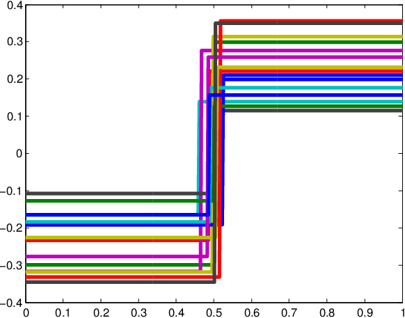
As a third example, we’d like to mention that spectral decomposition could also serve as a tool for collaboratively analyzing input data. Just to point out possible applications, Figure 5 shows two examples: The left part corresponds to an analysis of 15 different input signals with the collaborative sparse regularization . Similar to the DCT case, the problem decouples in one direction and yields regularized subproblems in each component. As we can see in the left part of figure 5, an ideal low-pass reconstruction yields exactly those peaks for which all input signals in had non-zero entries.
Similar concepts could also be derived for collaborative jumps as shown in the right of 5, in which we used . As we can see, a strong low-pass filter leads to the best single joint jump approximation in our example.



4 Conclusion
In this paper the theory of nonlinear spectral representation was generalized and extended in several ways. The framework of [16] was extended from the total variation functional to general one-homogeneous convex functionals. Analogue transform representations were formulated based on variational regularization and on inverse-scale-space [11] (in addition to the original gradient flow formulation). Moreover, an orthogonality of the decomposition is established and a new spectrum is suggested. Roughly, the spectrum measures the degree of activity of each scale. Here the spectrum is intrinsic to the functional space and can be viewed as a natural nonlinear extension of Parseval’s identity. Three examples of smoothing one-homogeneous functionals, other than TV, illustrate possible benefits of this approach for enhanced image and signal representation.
5 Acknowledgements
MB acknowledges support by ERC via Grant EU FP 7 - ERC Consolidator Grant 615216 LifeInverse.
References
- [1] Andreu, F., Ballester, C., Caselles, V., Mazón, J.M.: Minimizing total variation flow. Differential and Integral Equations 14(3), 321–360 (2001)
- [2] Andreu, F., Caselles, V., Dıaz, J., Mazón, J.: Some qualitative properties for the total variation flow. Journal of Functional Analysis 188(2), 516–547 (2002)
- [3] Aujol, J., Gilboa, G., Chan, T., Osher, S.: Structure-texture image decomposition – modeling, algorithms, and parameter selection. Int. J. Comp. Vision 67, 111–136 (2006)
- [4] Bartels, S., Nochetto, R., Abner, J., Salgado, A.: Discrete total variation flows without regularization. arXiv preprint arXiv:1212.1137 (2012)
- [5] Belkin, M., Niyogi, P.: Laplacian eigenmaps for dimensionality reduction and data representation. Neural computation 15(6), 1373–1396 (2003)
- [6] Bellettini, G., Caselles, V., Novaga, M.: The total variation flow in . Journal of Differential Equations 184(2), 475–525 (2002)
- [7] Benning, M., Brune, C., Burger, M., Müller, J.: Higher-order tv methods:enhancement via bregman iteration. J Sci Comput 54, 269–310 (2013)
- [8] Benning, M., Burger, M.: Ground states and singular vectors of convex variational regularization methods. Meth. Appl. Analysis 20(4), 295–334 (2013)
- [9] Bredies, K., Kunisch, K., Pock, T.: Total generalized variation. SIAM J. Imaging Sciences 3(3), 492–526 (2010)
- [10] Burger, M., Frick, K., Osher, S., Scherzer, O.: Inverse total variation flow. Multiscale Modeling & Simulation 6(2), 366–395 (2007)
- [11] Burger, M., Gilboa, G., Osher, S., Xu, J.: Nonlinear inverse scale space methods. Comm. in Math. Sci. 4(1), 179–212 (2006)
- [12] Chan, T.F., Osher, S., Shen, J.: The digital TV filter and nonlinear denoising. IEEE Trans. Image Process. 10(2), 231–241 (2001)
- [13] Eckardt, L.: Spektralzerlegung von Bildern mit TV-methoden (2014), bachelor thesis, University of Münster.
- [14] Giga, Y., Kohn, R.: Scale-invariant extinction time estimates for some singular diffusion equations. Hokkaido University Preprint Series in Mathematics (963) (2010)
- [15] Gilboa, G.: A spectral approach to total variation. In: A. Kuijper et al. (Eds.): SSVM 2013. LNCS, vol. 7893, pp. 36–47. Springer (2013)
- [16] Gilboa, G.: A total variation spectral framework for scale and texture analysis. SIAM J. Imaging Sciences 7(4), 1937–1961 (2014)
- [17] Liu, G., Lin, Z., Yan, S., Sun, J., Yu, Y., Ma, Y.: Robust recovery of subspace structures by low-rank representation. Pattern Analysis and Machine Intelligence, IEEE Transactions on 35(1), 171–184 (2013)
- [18] Meyer, Y.: Oscillating patterns in image processing and in some nonlinear evolution equations (2001)
- [19] Müller, J.: Advanced image reconstruction and denoising: Bregmanized (higher order) total variation and application in pet (2013), Ph.D. Thesis, Univ. Münster.
- [20] Ng, A., Jordan, M., Weiss, Y.: On spectral clustering: Analysis and an algorithm. Advances in neural information processing systems 2, 849–856 (2002)
- [21] Osher, S., Sole, A., Vese, L.: Image decomposition and restoration using total variation minimization and the H-1 norm. SIAM Multiscale Model. Simul. 1, 349–370 (2003)
- [22] Rudin, L., Osher, S., Fatemi, E.: Nonlinear total variation based noise removal algorithms. Physica D 60, 259–268 (1992)
- [23] Shi, J., Malik, J.: Normalized cuts and image segmentation. IEEE Transactions on Pattern Analysis and Machine Intelligence 22(8), 888–905 (2000)
- [24] Steidl, G., Weickert, J., Brox, T., Mr�zek, P., Welk, M.: On the equivalence of soft wavelet shrinkage, total variation diffusion, total variation regularization, and SIDEs. SIAM Journal on Numerical Analysis 42(2), 686–713 (2004)
- [25] Xu, J., Osher, S.: Iterative regularization and nonlinear inverse scale space applied to wavelet-based denoising. IEEE Trans. Image Processing 16(2), 534–544 (2007)