Hyperbolic Graph Generator
Abstract
Networks representing many complex systems in nature and society share some common structural properties like heterogeneous degree distributions and strong clustering. Recent research on network geometry has shown that those real networks can be adequately modeled as random geometric graphs in hyperbolic spaces. In this paper, we present a computer program to generate such graphs. Besides real-world-like networks, the program can generate random graphs from other well-known graph ensembles, such as the soft configuration model, random geometric graphs on a circle, or Erdős-Rényi random graphs. The simulations show a good match between the expected values of different network structural properties and the corresponding empirical values measured in generated graphs, confirming the accurate behavior of the program.
Keywords:
Complex networks , network geometry , graph theory , hyperbolic graphsPACS
89.75.Fb , 02.10.OxProgram summary
Program title: Hyperbolic Graph Generator
Program summary URL: http://named-data.github.io/Hyperbolic-Graph-Generator/
Licensing provisions: General Public License, version 3
Programming language: C++
Computer/Operating system: Any
Nature of problem: Generation of graphs in hyperbolic spaces.
Solution method: Implementation based on analytical equations.
Running time: Depends on the number of nodes. A few seconds for graph in the example provided.
Other features: Can be used as a command-line tool or installed as a library to support more complex software.
1 Introduction
The interactions between components of a complex system are often represented as a network. This modeling allows for rigorous mathematical treatment, and broadens our understanding of the system [1]. Many real networks possess common structural patterns, including, in the first place, heterogeneous (often power-law) distributions of node degrees [2], and strong clustering, i.e., higher numbers of triangular subgraphs than predicted by classical random graph models [3]. Recently introduced geometric graph models, based on the assumption that nodes in real networks are embedded in latent hyperbolic spaces [4, 5], reproduce these common structural properties of real networks. Furthermore, these hyperbolic graphs replicate dynamical processes on top of real networks [6] and accurately predict missing links in them [7].
| \diaghead(5,-2){zzzzzz}{{\footnotesize\shortstack[l]{$\gamma$}}}{{\footnotesize\shortstack[r]{$T$}}} | |||
|---|---|---|---|
| Hyperbolic RGGs | Soft hyperbolic RGGs | Soft configuration model | |
| Spherical RGGs | Soft spherical RGGs | Erdős-Rényi |
In this work we present a program to generate random hyperbolic graphs. This software implements and extends the network model introduced in [4]. Nodes are randomly sprinkled on a hyperbolic disk, and the probability of the existence of an edge (the connection probability) between two nodes is a function of the distance between the nodes in the hyperbolic space. Thus generated graphs have strong clustering, and node degree distributions in them are power laws. Moreover, other popular and well-studied random graph ensembles, namely the soft configuration model (SCM) [8], (soft) random geometric graphs (RGGs) on a circle [9, 10], and Erdős-Rényi (ER) random graphs [11], appear as degenerate regimes in the model. Table 1 shows all the model regimes, the total of six. Each regime is defined by the values of only two parameters: , which is the expected exponent of the power-law degree distribution, and temperature , the parameter controlling the strength of clustering in the network.
Researchers in different disciplines may benefit from the use of random hyperbolic graphs in their work. Yet the full implementation of the model and all its regimes is a tricky business, which involves dealing with some delicate details, due to a variety of internal parameters and their interactions over the six regimes. In Sections 2-4 we describe the implementation details of the model, including how all the parameters are calculated in each regime. A good match between the values of expected graph properties and their observed values in generated graphs is confirmed in Section 5.
2 Input parameters and coordinates
2.1 Input parameters
The program input parameters are the number of nodes , the target expected average degree of the network, the target expected power-law exponent of the degree distribution, and temperature . The combination of and values will define the graph ensemble from which generated networks are sampled (Table 1).
Given the input parameters, the graph generation process consists of three steps:
- 1.
- 2.
Assign to all nodes their angular and radial coordinates on the hyperbolic plane, Section 2.2.
- 3.
2.2 Coordinate sampling
The assignment of node coordinates is done as follows in all the six regimes.
Angular coordinates of nodes are assigned by sampling them uniformly at random from interval , i.e., the angular node density is uniform .
Radial coordinates , where is the radius of the hyperbolic disk, are sampled from the following distribution, which is nearly exponential with exponent ,
| (1) |
The calculation of internal parameter is described in detail below; it is different in different regimes. Internal parameter depends on the expected exponent of the power distribution of nodes degrees in generated graphs, and on the curvature of the hyperbolic space , which is set to by default. For temperatures , this relationship is given by
| (2) |
while for it becomes
| (3) |
To sample radial coordinates according to the distribution in Eq. (1), the inverse transform sampling is used: first a random value is sampled from the uniform distribution on , and then the radial coordinate of node is set to
| (4) |
3 Regimes with finite
3.1 : Soft hyperbolic random geometric graphs
This is the most general regime in the model, from which all other regimes can be obtained as limit cases. The connection probability in this case is
| (5) |
where , and is the radius of the hyperbolic disk occupied by nodes. The hyperbolic distance between two nodes at polar coordinates and is given by
| (6) |
where is the angular distance between the nodes. To calculate the expected degree of a node at radial coordinate , without loss of generality its angular coordinate can be set to zero, , so that its expected degree can be written as
| (7) |
The expected average degree in the network is then
| (8) |
Given user-specified values of input parameters , , and , the last equation is solved for using the bisection method in combination with numeric evaluation of the integrals in the equation. The MISER Monte Carlo algorithm from the GSL library is used to compute the multidimensional integral in Eq. (8). The iterative bisection procedure to find stops when the difference between the value of the computed integral in Eq. (8) and the target value of is smaller than a threshold that is set to by default.
3.2 Limit : Hyperbolic random geometric graphs
In the () limit, the connection probability in Eq. (5) becomes
| (9) |
where is the Heaviside step function, meaning that two nodes are connected if the hyperbolic distance between them is less than , or they are not connected otherwise. The expected average degree in the network is given by the same Eq. (8), but with in the last equation. The value of is determined using the same procedure as in Section 3.1. The only difference is that function is given by Eq. (9).
3.3 Limit : Soft configuration model
According to Eq. (3), in the limit with finite , to have finite , curvature should also go to infinity, , such that is finite, and instead of Eq. (3) one gets
| (10) |
More importantly, one can show that as a result of , the expression for hyperbolic distance between two nodes in Eq. (6) degenerates to
| (11) |
meaning that in the regime the angular coordinates are completely ignored. The connection probability becomes
| (12) |
and the expected average degree in the network is
| (13) |
The value of is determined using the same combination of the bisection method and numeric integration as in the previous section, except it is applied to Eq. (13).
4 Regimes with infinite
While in the limit the angular coordinates are ignored, in the limit the radial coordinates are ignored. One can show this formally by observing that in this limit the radial node density approaches a delta function—all nodes are placed at the boundary at infinity of the hyperbolic plane, meaning that only angular coordinates determine distances between nodes.
4.1 : Soft spherical random geometric graphs
In this most general case with infinite , one can show that the connection probability in Eq. (5) degenerates to
| (14) |
where is the angular distance between the two nodes as before, while is a parameter controlling the average degree in the network, analogous to in the regimes with finite . Without loss of generality we can set , so that the expression for is
| (15) |
where is the Gauss hypergeometric function, and . In the special case with , the last expression simplifies to
| (16) |
If , the hypergeometric function in Eq. (15) cannot be evaluated using the GSL library, because the evaluation in the library is implemented only for the case where the fourth argument of the function ( in Eq. (15)) is between and , while for sufficiently large , is always larger than in Eq. (15). To avoid this difficulty, the following transformation is used [12]:
| (17) |
If is an integer, the second term in (17) diverges due to the function in the denominator, while the first term diverges because the third parameter of the function is a non-positive integer. Hence, for integer values of temperature , their value is approximated by , where is set to by default. The error caused by this approximation is negligible. Equation (17) (or (16) if ) is then numerically solved for using the bisection method, yielding the target value of in Eq. (15).
| \diaghead(5,-2){zzzzzzzzzzzz}{{\footnotesize\shortstack[l]{$\,\gamma$}}}{{\footnotesize\shortstack[r]{$T$}}} | |||||
|---|---|---|---|---|---|
| 9.662.19 | 9.902.16 | 9.981.08 | 9.881.58 | 9.841.47 | |
| 10.080.11 | 10.010.10 | 10.020.04 | 10.000.08 | 9.990.09 | |
| 10.000.00 | 10.000.00 | 10.000.00 | 10.000.00 | 10.000.00 |
| \diaghead(5,-2){zzzzzzzzzzzz}{{\footnotesize\shortstack[l]{$\,\gamma$}}}{{\footnotesize\shortstack[r]{$T$}}} | |||||
|---|---|---|---|---|---|
| 0.880.00 | 0.750.00 | 0.290.00 | 0.360.01 | 0.360.01 | |
| 0.790.00 | 0.410.00 | 0.420.00 | 0.010.00 | 0.010.00 | |
| 0.750.00 | 0.330.00 | 0.300.00 | 0.000.00 | 0.000.00 |
4.2 Limit : Spherical random geometric graphs
One can see from Eq. (17) that the solution for at small scales with as , . Therefore for the connection probability in Eq. (14) can be written as
| (18) |
which in the limit becomes
| (19) |
meaning that two nodes are connected if the angular distance between them is smaller than ,
| (20) |
or they are not connected otherwise. This connectivity threshold ensures that the expected average degree in the network is .
4.3 Limit : Erdős-Rényi graphs
In this most degenerate regime, both angular and radial coordinates are completely ignored. This regime is formally achieved by keeping both and finite while letting . One can then show that the connection probability in Eq. (5) degenerates to
| (21) |
which for sparse graphs with tends to , i.e., the connection probability in classical (Erdős-Rényi) random graphs.
5 Simulations
Tables 2(a) and 2(b) show, respectively, the average degree and clustering values in generated graphs for different regimes, samples in each regime. All the regimes match the target average degree , although low values of lead to much higher fluctuations. For any , average clustering decreases with temperature from a maximum at to zero at .
Figure 1 shows the observed distribution of node degrees for three different values of . As expected, for finite , distributions follow a power-law . In the limit at the observed degree distributions follow exactly the Poisson distribution with mean .
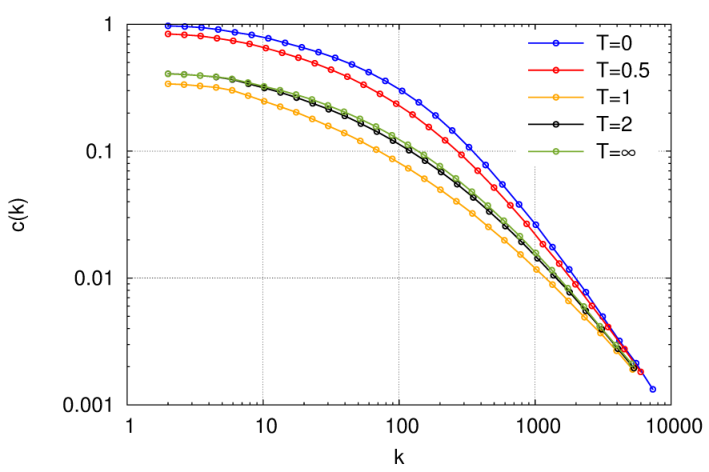
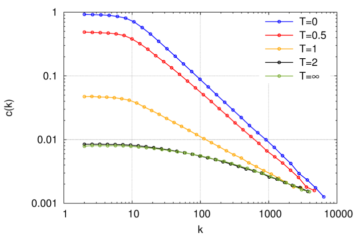
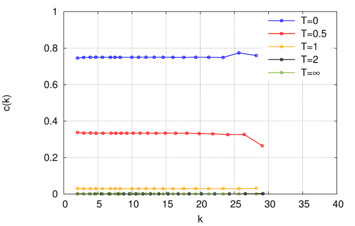
Figure 2 shows clustering in generated graphs. For finite , low-degree nodes have stronger clustering than high-degree nodes. In the case of , all nodes have similar clustering values.
Acknowledgments
This work supported by NSF Grants No. CCF-1212778, CNS-1441828, and CNS-1442999.


References
- [1] S. N. Dorogovtsev, Lectures on complex networks, vol. 24, Oxford University Press, Oxford, 2010.
- [2] A.-L. Barabási, R. Albert, Emergence of scaling in random networks, Science 286 (1999) 509–512.
- [3] M. Newman, Networks: An introduction, Oxford University Press, Oxford, 2010.
- [4] D. Krioukov, F. Papadopoulos, M. Kitsak, A. Vahdat, M. Boguñá, Hyperbolic geometry of complex networks, Phys Rev E 82 (2010) 036106.
- [5] F. Papadopoulos, M. Kitsak, M. Á. Serrano, M. Boguñá, D. Krioukov, Popularity versus similarity in growing networks, Nature 489 (2012) 537–540.
- [6] M. Boguñá, F. Papadopoulos, D. Krioukov, Sustaining the Internet with hyperbolic mapping, Nat Comm 1 (2010) 62.
- [7] F. Papadopoulos, C. Psomas, D. Krioukov, Network mapping by replaying hyperbolic growth, IEEE ACM T Netw 23 (2014) 198–211.
- [8] J. Park, M. Newman, Statistical mechanics of networks, Phys Rev E 70 (2004) 066117.
- [9] M. D. Penrose, Random geometric graphs, vol. 5, Oxford University Press, Oxford, 2003.
- [10] M. D. Penrose, Connectivity of soft random geometric graphs, arXiv:1311.3897 .
- [11] P. Erdős, A. Rényi, On random graphs, Pub Math Deb 6 (1959) 290–297.
- [12] R. C. Forrey, Computing the hypergeometric function, J Comp Phys 137 (1997) 79–100.