Coupled wire construction of chiral spin liquids

Introduction.—The experimental discovery [1] and conceptual understanding [2] of the fractional quantum Hall effect (FQHE) had a tremendous impact on contemporary research of strongly correlated electron systems. In particular, it triggered interest in topologically ordered quantum states of matter, which since then have persisted as a predominant focus. Following up on an idea by D. H. Lee, Kalmeyer and Laughlin [3, 4] proposed the chiral spin liquid [5, 6] (CSL) as a fractionally quantized Hall liquid for bosonic spin flip operators acting on a spin-polarized reference state. Fractionalization of charge for FQHE relates to fractionalization of spin for the CSL, which supports $S=1/2$ spinons obeying half-Fermi statistics [7]. The CSL has been an invaluable seed for new concepts such as topological order [8], providing a direct perspective on the fundamental relations between FQHE, spin liquids, and superconductivity [5, 9]. Despite its high relevance as a paradigm formulated via wave functions, the first Hamiltonian for which the CSL is the (aside from topological degeneracies) unique ground state was only identified two decades after the liquid had been proposed [10]. The approach was subsequently expanded to yield different classes of such trial Hamiltonians [11], where the latest and more generic versions are more short-ranged than the initial microscopic models: they involve 2-body and 3-body spin interactions which can be deduced from the explicit construction of appropriate annihilation operators [12] or null operators in conformal field theory [13]. In particular, non-Abelian chiral spin liquids with level $k$ parafermionic spin excitations have been proposed [14, 12], which nurture the hope for alternative scenarios of topological quantum computation in frustrated magnets and Mott regimes of alkaline earth atoms deposited in optical lattices [15, 16].

Since their discovery, CSLs have been appreciated as a realisation of a bosonic Laughlin state at Landau level filling fraction $\nu=1/2$ on a spin lattice. Naturally, the CSL of Refs. 3, 4 can be defined on any lattice [17, 18], which becomes mathematically transparent via the generalized Perelomov identity [19] for lattices with a primitive unit cell. Some of these motifs have later reappeared in the field of fractional Chern insulators [20, 21, 22]. As of today, several promising CSL scenarios with broken SU(2) spin symmetry have been proposed, while analytic wave functions are not known in these cases. The most important one is the Kitaev model on the decorated honeycomb lattice [23], which can be solved exactly by a mapping to Majorana fermions. In addition, recent large-scale numerical studies are interpreted in favor of a CSL regime in models of broken [24] and conserved [25, 26, 27, 28] SU(2) spin symmetry on the kagome lattice, where competing magnetic order is sufficiently frustrated. From the viewpoint of symmetry classification, SU(2) symmetry is not a characteristic feature of CSLs. In contrast, parity (P) and time-reversal (T) symmetry are necessarily broken in CSLs, and they support (gaped) spinon excitations in an otherwise featureless fluid.

In this Letter, we develop a coupled wire construction (CWC) of CSL states. The CWC for topologically ordered quantum states of matter originates from the pioneering work by Kane and collaborators on deriving a scenario of FQH states from suitably chosen many-particle couplings in a set of coupled quantum wires [29]. Important preceding work has been on sliding Luttinger liquid phases, which already installed the notion of using the magnetic field as a way to favorably tune the scaling dimension of inter-wire couplings [30]. Recently, the CWC of two-dimensional systems has been employed in various contexts [31, 32, 33, 34, 35, 37, 38, 36, 39] including a derivation of the periodic table of integer and fractional fermionic topological phases [40]. In a way, the CWC of Abelian and non-Abelian CSLs reported in this paper completes the program previously pursued for the CWC of Read-Rezayi states in the FQHE [41, 42] and their superconducting analogues [43, 44]. As such, the CWC provides a fruitful perspective on a broad range of non-Abelian topological quantum states of matter.

Model of coupled wires.—We analyze a $k$-fold stacked array of $N$ quantum wires, as shown in Fig. 1. We label the wires by $(a,b)$, where $a=1,\ldots,k$ is the layer (or flavour) index, and $b=1,\ldots,N$ is the wire index within each layer. Each wire is modeled by a cosine band of spinful electrons, subject to a Zeeman field and spin-orbit coupling. The couplings are constant within a given wire, but depend on the wire index $b$. The four Fermi points of right (R) and left (L) moving electrons of spin $\sigma=\,\uparrow,\downarrow$ in wire $(ab)$ reside at momenta

where $r=\text{R},\text{L}$. We identify $\text{R},\uparrow\,\equiv+$ and $\text{L},\downarrow\,\equiv-$. Here, $k_{\text{F}}$ denotes the bare Fermi momentum, and $k_{\text{Z}}^{(b)}$ and $k_{\text{so}}^{(b)}$ the momentum shifts due to the Zeeman field and the spin-orbit coupling, respectively.

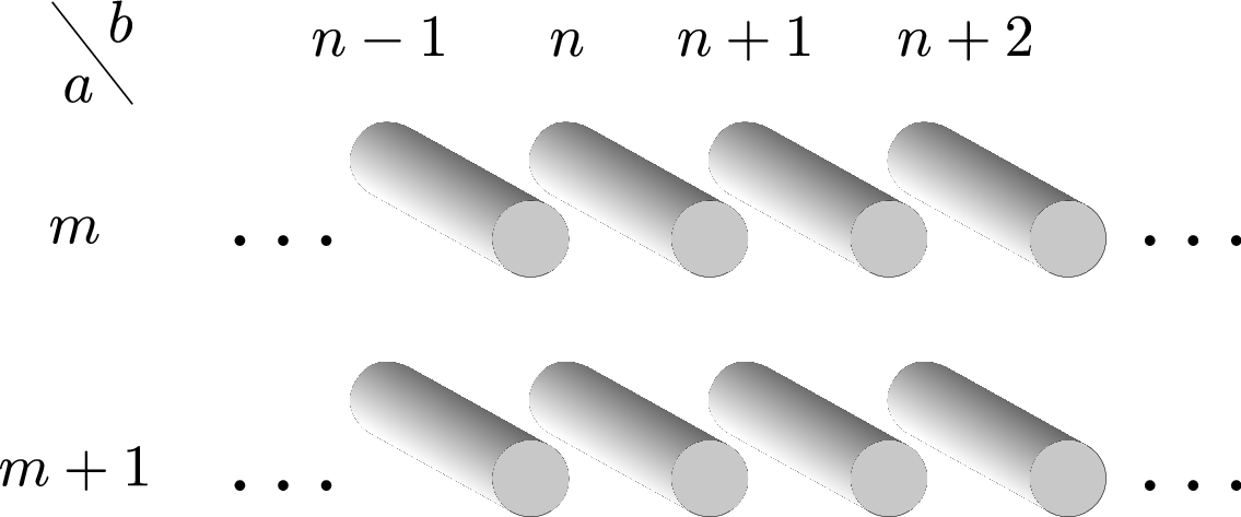
Throughout this paper, we treat the system in (Abelian) bosonization [45]. Linearising the spectrum around the Fermi points, the electron annihilation operators $c_{\sigma}^{(ab)}(x)$ can be decomposed into right and left moving modes,

which we bosonize as

where $U_{r\sigma}^{(ab)}$ is a Klein factor, and $\alpha$ the short distance cutoff of the theory. The bosonic fields obey

With these definitions, the long wavelength density fluctuations of spin $\sigma$ electrons in wire $(ab)$ are given by $\rho_{\sigma}^{(ab)}(x)=-\frac{1}{\pi}\partial_{x}\phi_{\sigma}^{(ab)}(x)$. In terms of the charge c and spin s modes of the wires, defined as

the Hamiltonian density of an individual wire reads

where the $(4\times 4)$-matrix $V_{ab}$ depends on the Fermi velocity and forward scattering interactions, and $\Psi_{ab}=(\partial_{x}\phi_{c}^{(ab)},\partial_{x}\phi_{\text{s}}^{(ab)},\partial_{x}\theta_{c}^{(ab)},\partial_{x}\theta_{\text{s}}^{(ab)})^{T}$. In addition to the quadratic part, the Hamiltonian also contains a Mott term $\sim g_{3}$, and a backscattering term $\sim g_{1\perp}$. In a clean system, these terms contribute only when the oscillating prefactors vanish.

Mott gap and spin flip operators.—For the construction of a spin liquid, we gap out the charge sector in each wire by tuning it into the Mott regime. Equation 6 implies that this regime can be reached for $\sum_{r\sigma}k_{\text{F}r\sigma}^{(b)}=2\pi/\alpha_{0}$, where $\alpha_{0}$ is the lattice constant (taken identical in all wires). We thus demand $k_{\text{F}}=\pi/2\alpha_{0}$. At the same time, the spin sectors should remain gapless if there are no inter-wire couplings. This either requires the sine-Gordon term $\sim g_{1\perp}$ to be irrelevant in the sense of the renormalization group (RG) (or less relevant than the couplings stabilizing the spin liquids, which are discussed below), or $\sum_{r\sigma}\sigma k_{\text{F}r\sigma}^{(ab)}=4k_{\text{Z}}^{(ab)}\neq 0$. We thus apply a Zeeman field in all wires.

In the Mott phase, the single wire Hamiltonian densities $\mathcal{H}_{0}^{(ab)}$ pin the fields $\phi_{c}^{(ab)}$ to values $\phi_{c}^{(ab)}\approx\langle\phi_{c}^{(ab)}\rangle$. (The value of $\langle\phi_{c}^{(ab)}\rangle$ depends on the sign convention for the ordering of the Klein factors. Taking them to be Majorana fermions with $U_{r\sigma}^{\dagger}=U_{r\sigma}$ and $U_{r\sigma}^{2}=1$, we choose $U_{\text{L}\uparrow}U_{\text{L}\downarrow}U_{\text{R}\uparrow}U_{\text{R}\downarrow}=1$ on each wire $(ab)$. A Hubbard interaction $Uc_{\uparrow}^{\dagger}c_{\uparrow}^{\phantom{\dagger}}c_{\downarrow}^{\dagger}c_{\downarrow}^{\phantom{\dagger}}$ then generates $g_{3}=-U<0$, which implies we may take $\langle\phi_{c}^{(ab)}\rangle=0$.)

In the Mott phase, the remaining local degrees of freedom are spin flip operators

where

Abelian chiral spin liquid.—The Abelian CSL only requires a single layer, or flavour, of wires ($k=1$). Similar to the wire construction of quantum Hall states [29, 42], we couple right movers in wire $b$ to left movers in wire $b+1$, but not in wire $b-1$. Such a coupling breaks time reversal symmetry T as well as two-dimensional parity P (which we take as $x\to x$, $y\to-y$ along and transverse to the wires, respectively), but is PT invariant. (The conservation of PT, however, is no prerequisite for a CSL in the sense of a symmetry-protected topological (SPT) phase [31].)

In the construction of Kalmeyer and Laughlin [3, 4] (KL), P and T are violated through the fictitious magnetic field used to stabilise the $m=2$ Laughlin state, which is then projected to describe spin flips on a lattice commensurable with the magnetic field (one Dirac flux quantum per unit cell of the square lattice). While readily implemented in a language of wave functions, this method of obtaining a CSL state in two steps—writing it out in the continuum and then projecting it onto the lattice—is not available in a description in terms of Hamiltonians, such as our CWC. In all known constructions [10, 11, 12, 13] of parent Hamiltonians of the KL state, P and T violation is implemented through a three-spin interaction of the form $\bm{S}_{i}(\bm{S}_{j}\times\bm{S}_{k})$, where $i$, $j$, and $k$ are three lattice sites on a plaquette.

A term of this form, however, is not easily implemented as a coupling between wires. A simpler and more elegant way to obtain a CSL, i.e., to install the desired couplings between right movers in wire $b$ to left movers of wire $b+1$, is to adjust the values for $k_{\text{Z}}$ and $k_{\text{so}}$ such that all the terms in $S_{1b}^{+}S_{1b+1}^{-}$, except the desired ones, oscillate, i.e.,

while no other values for $k_{1r}$ or $k_{2r}$ match between neighboring wires. P violation, as defined above, requires the unit cell to contain more than 2 wires. A possible choice for $k_{\text{Z}}$ and $k_{\text{so}}$ within a 3-wire unit cell is given in Tab. 1, and results in the spin flip momenta $k_{1r}^{(1b)}$ and $k_{2r}^{(1b)}$ of Tab. 2. The price we pay for the simplicity of the construction is that the Zeeman and spin-orbit couplings violate SU(2) spin symmetry at the single wire level, which is intact in the KL liquid, but not a required property for the universality class of CSLs [23, 24].

In terms of bosonic fields, a coupling $\frac{1}{2}J(S_{ab}^{+}S_{a^{\prime}b+1}^{-}+\text{H.c.})$ between neighboring wires yields the transverse Hamiltonian densities

with $2t=J/(2\pi\alpha)^{2}$. These terms commute with themselves at different positions $x$ along the wires (which implies that they can pin the value of the field combinations forming their argument, and hence open up an energy gap), and with each other for different values of $b$. The full Hamiltonian for the wire-coupled Abelian ($k=1$) CSL is hence given by

The state is gapped in the bulk but supports gapless chiral edge modes in wires $1$ and $N$, which are described by the bosonic fields $\Phi_{1}(x)=\bigl(-\phi_{\text{s}}^{(11)}(x)-\theta_{\text{s}}^{(11)}(x)\bigr)/\sqrt{2}$ and $\Phi_{N}(x)=\bigl(\phi_{\text{s}}^{(1N)}(x)-\theta_{\text{s}}^{(1N)}(x)\bigr)/\sqrt{2}$. The corresponding spin flip operators adding spin 1 to the edges can be defined as $S^{+}_{1}=\exp(2\text{i}\Phi_{1})$ and $S_{N}^{+}=\exp(2\text{i}\Phi_{N})$. Since the bosonic fields obey the commutation relations $[\Phi_{1}(x),\Phi_{1}(x^{\prime})]=-(\text{i}\pi/2)\text{sgn}(x-x^{\prime})$ and $[\Phi_{N}(x),\Phi_{N}(x^{\prime})]=(\text{i}\pi/2)\text{sgn}(x-x^{\prime})$, we can identify the mode $\Phi_{1}$ ($\Phi_{N}$) as a left (right) mover with a $K$-matrix of $K=-2$ ($+2$). This implies half-Fermi (also known as semion) statistics [7, 46].

The model further supports gapped bulk excitations described by $2\pi$-kinks in a sine-Gordon coupling of two neighboring chains (10). Since the total spin of the system is given by

modulo edge terms, the spin associated with a kink is $S^{\text{z}}=1/2$. The kinks describe spinon excitations, which are fractionalized as the Hilbert space for a spin 1/2 Mott isolator is spanned by spin flips operators with $S^{\text{z}}=1$, which act on a spin polarized vacuum.

Non-Abelian chiral spin liquids.—We now consider $k>1$ flavors (or layers) of coupled wires (as illustrated in Fig. 1), and assume $k_{\text{Z}}$ and $k_{\text{so}}$ as specified in Tab. 1 for all flavors. Spin-spin couplings between neighboring wires yield three types of cosine terms of Hamiltonian densities, which do not commute mutually, but preserve momentum and do commute with themselves at different positions $x$ along the wire. (In practise, the latter condition implies that we only need to consider terms which contain two left movers and two right movers, regardless of whether they stem from creation or annihilation operators, when we expand four fermion couplings.)

The first type is as given in Eq. (10), which we allow for all $a,a^{\prime}=1,\ldots,k$ with the same coefficient $t$. (Note that the commutator between $\mathcal{H}_{t}^{(aa^{\prime}b)}(x)$ and $\mathcal{H}_{t}^{(cc^{\prime}b)}(x^{\prime})$ vanishes only if either $(a,a^{\prime})=(c,c^{\prime})$ or $a\neq c\wedge a^{\prime}\neq c^{\prime}$.) The second type is generated by the coupling $\frac{1}{2}J_{\text{x}\text{y}}(S_{ab}^{+}S_{a^{\prime}b}^{-}+\text{H.c.})$ between different flavors $a$ and $a^{\prime}$ on the same wire $b$ and takes the form

with $u=-2J_{\text{x}\text{y}}/(2\pi\alpha)^{2}$. (The relative sign between terms with different Klein factors can be determined by insertion of $U_{\text{L}\uparrow}U_{\text{L}\downarrow}U_{\text{R}\uparrow}U_{\text{R}\downarrow}=1$.) Finally, the third type is generated by the coupling $J_{\text{z}}S_{ab}^{\text{z}}S_{a^{\prime}b}^{\text{z}}$ of the operators

between different flavors $a,a^{\prime}$ on the same wire $b$, and is given by

with $v=-J_{\text{z}}/(2\pi\alpha)^{2}$. (Note that if the couplings are SU(2) symmetric, i.e., $J_{\text{x}\text{y}}=J_{\text{z}}$, one finds $u=2v$ in accordance with the energy density of $S^{\text{x}}S^{\text{x}}+S^{\text{y}}S^{\text{y}}$ being twice that of $S^{\text{z}}S^{\text{z}}$.)

The final Hamiltonian for the non-Abelian CSL at level $k$ is

A Hamiltonian related to Eq. (16) has been analyzed by Teo and Kane [42] in the context of their CWC of Abelian and non-Abelian FQH states. For $k=2$, it yields a Moore-Read (MR) [47] phase, and a strong pairing phase of charge $2e$ bosons at $\nu=1/4$ depending on the parameters $t$, $u$, and $v$. While the generic problem is intractable due to the non-commutativity of the different cosine terms, the phase diagram can still be obtained from the decoupling of individual composite modes in each wire. (Teo and Kane [42] assume the adjustment of forward scattering terms in their analogous form of Eq. (16) in such a way that the cosine field arguments decouple at the level of $\mathcal{H}_{0}$, and allow for refermionization of their free chiral spin fields represented by pairs of Majorana fermions. For $k=2$, this analysis transparently resolves the MR and the strong pairing phase depending on how the Majorana modes are paired between or within the wires.) As such, this allows for an effective implementation of the coset construction in conformal field theory, which then can be used to yield parafermionic topological phases from the CWC. In particular, if we choose the bare coupling parameter $u=v$ (i.e., we set $J_{\text{z}}=2J_{\text{x}\text{y}}$), the analysis implies that we stabilize a non-Abelian SU(2) level ${k=2}$ CSL [14], which may be viewed as the spin liquid pendant to the MR state. For arbitrary $k$ and $u=v$ (but regardless of $t$), the same procedure yields a non-Abelian CSL with level $k$ parafermionic edge modes. This phase constitutes the coupled wire pendant of the SU(2)_k non-Abelian CSL [14], which, on the level of wave functions, is obtained from the symmetrization of $k$ Abelian CSLs in the layers. We should note at this point, however, that an equality of the bare couplings $u$ and $v$ in Eq. (16) does not guarantee that they remain equal under the RG flow towards lower energies. Whether the SU(2)_k parafermionic CSL is the RG fixed point for a given bare parameter setup depends on the relative coupling strengths of the cosine terms, and the forward scattering amplitudes.

Conclusion and Outlook.—The coupled wire construction of Abelian and non-Abelian chiral spin liquids offers a deconstructivist and yet physically motivated, microscopic view on these unconventional topological quantum states of matter. For the Abelian state, starting from bosonic spin flip operators which carry spin 1 and couple the Mott-gaped wires, we have constructed a topological phase with a bulk gap, fractionalized spin $1/2$ bulk quasiparticles (i.e., spinons), and a single chiral edge mode. We identify this phase with a chiral spin liquid, and the generalization to multiple layers with SU(2)_k parafermionic chiral spin liquids. The construction outlined above constitutes the starting point for further study. First, the nature of the bulk, and in particular the edge, excitations of the SU(2)_k chiral spin liquids require further investigation. Second, a more rigorous RG treatment of (16) is indispensable in acquiring an understanding of the phase diagrams of multi-layer Mott-gapped wires as well as to assess the range of stability for the SU(2)_k chiral spin liquid states. For $k>2$, this has so far not even been attempted for the analogous FQHE scenario, and might yield new insights. Third, from the construction outlined in this Letter, we might also be able to construct spin liquids without P and T breaking, i.e., the spin liquid pendants [48, 49] of a fractional topological insulator [50].

We thank M. Barkeshli, B. Bauer, E. Fradkin, and A. W. W. Ludwig for discussions. This work has been funded by the Helmholtz association through VI-521, the DFG through SFB 1143, and the European Research Council through ERC-StG-TOPOLECTRICS-336012. T.N. acknowledges financial support from DARPA SPAWARSYSCEN Pacific N66001-11-1-4110.

Note added: In the final stages of this work, we became aware that a similar idea is being pursued by G. Gorohovsky, R. G. Pereira, and E. Sela [51].

References

- [1] D. C. Tsui, H. L. Stormer, and A. C. Gossard, Phys. Rev. Lett. 48, 1559 (1982).
- [2] R. B. Laughlin, Phys. Rev. Lett. 50, 1395 (1983).
- [3] V. Kalmeyer and R. B. Laughlin, Phys. Rev. Lett. 59, 2095 (1987).
- [4] V. Kalmeyer and R. B. Laughlin, Phys. Rev. B 39, 11879 (1989).
- [5] X. G. Wen, F. Wilczek, and A. Zee, Phys. Rev. B 39, 11413 (1989).
- [6] R. B. Laughlin and Z. Zou, Phys. Rev. B 41, 664 (1990).
- [7] F. Wilczek, Fractional statistics and anyon superconductivity (World Scientific, Singapore, 1990).
- [8] X. G. Wen, Phys. Rev. B 40, 7387 (1989).
- [9] N. Read and D. Green, Phys. Rev. B 61, 10267 (2000).
- [10] D. F. Schroeter, E. Kapit, R. Thomale, and M. Greiter, Phys. Rev. Lett. 99, 097202 (2007).
- [11] R. Thomale, E. Kapit, D. F. Schroeter, and M. Greiter, Phys. Rev. B 80, 104406 (2009).
- [12] M. Greiter, D. F. Schroeter, and R. Thomale, Phys. Rev. B 89, 165125 (2014).
- [13] A. E. B. Nielsen, J. I. Cirac, and G. Sierra, Phys. Rev. Lett. 108, 257206 (2012).
- [14] M. Greiter and R. Thomale, Phys. Rev. Lett. 102, 207203 (2009).
- [15] M. Hermele, V. Gurarie, and A. M. Rey, Phys. Rev. Lett. 103, 135301 (2009).
- [16] A. E. B. Nielsen, G. Sierra, and I. Cirac, Nature Communications 4, 2864 (2013).
- [17] Z. Zou, B. Doucot, and B. S. Shastry, Phys. Rev. B 39, 11424 (1989).
- [18] K. Yang, L. K. Warman, and S. M. Girvin, Phys. Rev. Lett. 70, 2641 (1993).
- [19] M. Greiter and R. Thomale, Phys. Rev. B 85, 155145 (2012).
- [20] E. Tang, J.-W. Mei, and X.-G. Wen, Phys. Rev. Lett. 106, 236802 (2011).
- [21] K. Sun, Z. Gu, H. Katsura, and S. Das Sarma, Phys. Rev. Lett. 106, 236803 (2011).
- [22] T. Neupert, L. Santos, C. Chamon, and C. Mudry, Phys. Rev. Lett. 106, 236804 (2011).
- [23] H. Yao and S. A. Kivelson, Phys. Rev. Lett. 99, 247203 (2007).
- [24] S.-S. Gong, W. Zhu, L. Balents, and D. N. Sheng, Phys. Rev. B 91, 075112 (2015).
- [25] L. Messio, B. Bernu, and C. Lhuillier, Phys. Rev. Lett. 108, 207204 (2012).
- [26] B. Bauer, L. Cincio, B. P. Keller, M. Dolfi, G. Vidal, S. Trebst, and A. W. W. Ludwig, Nature Communications 5, 5137 (2014).
- [27] W.-J. Hu, W. Zhu, Y. Zhang, S. Gong, F. Becca, and D. N. Sheng, Phys. Rev. B 91, 041124 (2015).
- [28] A. Wietek, A. Sterdyniak, and A. Läuchli, arXiv:1503.03389.
- [29] C. L. Kane, R. Mukhopadhyay, and T. C. Lubensky, Phys. Rev. Lett. 88, 036401 (2002).
- [30] S. L. Sondhi and K. Yang, Phys. Rev. B 63, 054430 (2001).
- [31] Y.-M. Lu and A. Vishwanath, Phys. Rev. B 86, 125119 (2012).
- [32] A. Vaezi and M. Barkeshli, Phys. Rev. Lett. 113, 236804 (2014).
- [33] I. Seroussi, E. Berg, and Y. Oreg, Phys. Rev. B 89, 104523 (2014).
- [34] J. Klinovaja and D. Loss, Eur. Phys. J. B 87, 171 (2014).
- [35] T. Meng, P. Stano, J. Klinovaja, and D. Loss, Eur. Phys. J. B 87, 203 (2014).
- [36] J. Klinovaja and Y. Tserkovnyak, Phys. Rev. B 90, 115426 (2014).
- [37] E. Sagi and Y. Oreg, Phys. Rev. B 90, 201102 (2014).
- [38] T. Meng and E. Sela, Phys. Rev. B 90, 235425 (2014).
- [39] J. Klinovaja, Y. Tserkovnyak, and D. Loss. Phys. Rev. B 91, 085426 (2015).
- [40] T. Neupert, C. Chamon, C. Mudry, and R. Thomale, Phys. Rev. B 90, 205101 (2014).
- [41] N. Read and E. Rezayi, Phys. Rev. B 59, 8084 (1999).
- [42] J. C. Y. Teo and C. L. Kane, Phys. Rev. B 89, 085101 (2014).
- [43] R. S. K. Mong, D. J. Clarke, J. Alicea, N. H. Lindner, P. Fendley, C. Nayak, Y. Oreg, A. Stern, E. Berg, K. Shtengel, and M. P. A. Fisher, Phys. Rev. X 4, 011036 (2014).
- [44] A. Vaezi, Phys. Rev. X 4, 031009 (2014).
- [45] T. Giamarchi, Quantum Physics in One Dimension (Oxford University Press, Oxford, 2004).
- [46] X. Wen, Quantum Field Theory of Many-Body Systems, Oxford Graduate Texts (Oxford University, New York, 2004).
- [47] G. Moore and N. Read, Nucl. Phys. B 360, 362 (1991).
- [48] M. Greiter, J. Low Temp. Phys. 126, 1029 (2002).
- [49] B. Scharfenberger, R. Thomale, and M. Greiter, Phys. Rev. B 84, 140404 (2011).
- [50] M. Levin and A. Stern, Phys. Rev. Lett. 103, 196803 (2009).
- [51] G. Gorohovsky, R. G. Pereira, and E. Sela, submitted to arXiv.