The two-loop helicity amplitudes for
Abstract
We compute the two-loop massless QCD corrections to the helicity amplitudes for the production of two massive vector bosons in quark-antiquark annihilation, allowing for an arbitrary virtuality of the vector bosons: . Combining with the leptonic decay currents, we obtain the full two-loop QCD description of the corresponding electroweak four-lepton production processes. The calculation is performed by projecting the two-loop diagrams onto an appropriate basis of Lorentz structures. All two-loop Feynman integrals are reduced to a basis of master integrals, which are then computed using the differential equations method and optimised for numerical performance. We provide a public C++ code which allows for fast and precise numerical evaluations of the amplitudes.
Keywords
QCD, Collider Physics, NLO and NNLO Calculations1 Introduction
Vector boson pair production is an outstandingly important process at high energy hadron colliders. Its measurement allows precision studies of the electroweak interaction, thereby testing in detail the gauge structure and the matter content of the Standard Model of particle physics. The various combinations of vector boson pairs (, , , , , ) lead to spectacular final state signatures (leptons, photons, missing energy), that are often equally relevant to searches for new physics or studies of the Higgs boson. The Higgs boson decay into two vector bosons is among the cleanest signatures for Higgs production, and offers a broad spectrum of observables.
Precision studies of the electroweak interaction often focus on the pair production of on-shell gauge bosons, while new physics searches and Higgs boson studies precisely veto these on-shell contributions, such that the remaining background processes are dominated by off-shell gauge boson pair production. For both on-shell and off-shell production processes, it is therefore very important to have a precise prediction of the Standard Model contributions, in order to match the anticipated experimental accuracy of measurements at the LHC, which is usually in the per-cent range. At this level of precision, next-to-leading order (NLO) corrections in the electroweak theory and next-to-next-to-leading order (NNLO) corrections in QCD are indispensable.
For all vector boson pair production processes, NLO QCD corrections [1, 2, 3, 4, 5, 6] as well as large parts of the NLO electroweak corrections [7, 8, 9, 10, 11, 12, 13, 14] are available. These calculations are fully differential in all kinematical variables, and usually include the leptonic decays of the vector bosons. The derivation of NNLO QCD corrections to vector boson pair production can build upon calculational techniques [15, 16] that were originally developed for the Drell-Yan process [17, 18] or for Higgs boson production in gluon fusion [15, 16], which have the same QCD structure due to their colour-neutral final state. As a new ingredient, each vector boson pair production process at NNLO requires the two-loop corrections to the basic scattering amplitude for quark-antiquark annihilation: . These have been known for a while already for [19, 20] and [21, 22] production, enabling the calculations of these processes [23, 24] to NNLO accuracy.
Compared to the above, the two-loop matrix elements for the production of a pair of massive vector bosons require a new class of two-loop Feynman integrals: two-loop four-point functions with massless internal propagators and two massive external legs. Recently, very important progress has been made on these. For the case of equal vector boson mass, these integrals were derived in [25, 26], and used subsequently to compute the NNLO corrections to the on-shell production of [27] and [28]. The integrals for the most general case of non-equal masses were derived in [29, 30, 31], which allowed to construct the full two-loop helicity amplitude for in [32]. A subset of these integrals was derived independently in [33, 34] and used in the derivation of the fermionic NNLO corrections to production [34]. In this paper, we perform an independent rederivation of these integrals and optimise our solutions for numerical performance. They are used subsequently for a validation of the two-loop helicity amplitudes of [32], uncovering an error in their original results. We present a public implementation for the numerical evaluation of these amplitudes, which in the future will allow the calculation of NNLO QCD corrections to arbitrary electroweak four-fermion production processes.
The paper is structured as follows: in Section 2, we introduce the partonic current for vector boson pair production and describe its decomposition into Lorentz structures. Taking into account the vector boson decays into leptons, we present the helicity amplitudes for four particle final state in Section 3. A detailed description of the calculation and the different contributions to the amplitude is given in Section 4. The computation of the master integrals and their optimisation is presented in 5. In Section 6, we describe the subtraction of UV and IR counter terms, and in Section 7 we list the numerous checks we performed on our results. In Section 8 we present our C++ implementation for the numerical evaluation of the amplitudes and use it to produce numerical results. Finally, we conclude in Section 9. In Appendix A, we document the interference of the two-loop and tree amplitudes for the production of on-shell vector boson pairs, which was used in the calculation of the NNLO corrections to [27] and [28]. Appendix B contains the derivation of Schouten identities for the leptonic amplitudes, and Appendix C describes the conversion of our results between different schemes for the subtraction of infrared singularities. We provide computer readable files for our analytical results and our C++ code for the numerical evaluation of the amplitude on our VVamp project page on HepForge at http://vvamp.hepforge.org.
2 Lorentz structure of the partonic current for
Let us consider the production of two massive electroweak vector bosons in annihilation:
| (1) |
with
| (2) |
where the two vector bosons are off-shell and = , , , , , . We define the usual Mandelstam variables
| (3) |
such that
The physical region of phase space is bounded by such that
| (4) |
where is the Källén function
| (5) |
Let us consider the partonic amplitude for the production of the two off-shell vector bosons
| (6) |
where and are the two polarisation vectors of and respectively. In this notation, we keep an overall factor implicit, where is the positron charge.
In order to calculate the partonic current , we consider its tensorial structure. Lorentz invariance restricts it to be a linear combination of independent structures
| (7) |
where the form factors are scalar functions of the Mandelstam variables and of the number of space-time dimensions . To further constrain , we choose the Landau gauge for the electroweak vector bosons with the transversality condition
| (8) |
and the sum over polarisations
| (9) |
Imposing condition (8) we can reduce the number of independent tensor structures to ten [35, 36], which can be chosen as
| (10) |
Without any loss of generality we can thus write the partonic current as
| (11) |
where we introduced the new physical form factors , which are again scalar functions of the Mandelstam variables and of the dimension .
Note that in deriving (11) no assumption has been made on the dimensionality , such that this decomposition is valid for any continuous values of . Its structure has been constrained using solely Lorentz and gauge invariance and is therefore true at every order in perturbation theory. On the other hand, the scalar coefficients contain the explicit dependence on the perturbative order at which they are computed. These coefficients can be extracted from the amplitude by applying appropriate projecting operators on the latter. The projectors themselves can be expanded in the same tensorial basis:
| (12) |
where the coefficients are functions of the Mandelstam variables and of the dimension . They can be determined imposing that
| (13) |
Note that the contraction is performed in dimensions and at every stage one should always recall to use the polarisation sum in (9). For later convenience we introduce also the following scalar quantities:
| (14) |
which are related to the coefficients according to
| (15) |
with the same coefficients as in (12). These quantities (rather than the coefficients ) are particularly useful in order to build up the contractions of the -loop amplitudes with the tree-level ones (see Appendix A). We provide explicit expressions for in computer readable format on HepForge.
The partonic current receives contributions from QCD radiative corrections and can be decomposed perturbatively as
| (16) |
Obviously also the un-renormalised tensor coefficients (or, equivalently the ) have the same perturbative expansion of the partonic amplitude
| (17) | ||||
| (18) |
where the dependence on the Mandelstam variables is again implicit.
3 Helicity amplitudes for
In physical applications we are interested in the processes
| (19) |
where each of the two off-shell electroweak vector bosons can decay to pairs of leptons, such that and . Let us first focus on the general structure of the helicity amplitudes for this process. Schematically these amplitudes can be written as the product of the partonic current , and two leptonic currents , mediated by the propagators of the two off-shell vector bosons
| (20) |
where we stripped off electroweak couplings not relevant here and postpone their discussion to the presentation of the full amplitude in (36) below. In the -gauges the propagator of a vector boson reads
| (21) |
with
| (22) |
| (23) |
where is the mass of the gauge boson and is its decay width. While the Landau gauge used in the previous Section corresponds to , the term proportional to effectively vanishes for any since the electroweak vector bosons are directly coupled to massless fermion lines.
By fixing the helicities of the incoming partons and of the outgoing leptons one sees that the left- and right-handed partonic production currents can be written as
| (24) | ||||
| (25) |
where the are rank two-tensors and contain an odd number of -matrices. We note in passing that, by complex conjugation, one gets
The left- and right-handed leptonic decay currents, on the other hand, can be written as
| (26) | ||||
| (27) |
Note in particular that, as far as the lepton currents are concerned, a permutation of the external momenta corresponds to a flip of the helicity. All possible helicity amplitudes can be therefore obtained from the two basic amplitudes
| (28) | ||||
| (29) |
by simple permutations of the leptonic momenta. In particular we find
| (30) |
In order to put together the helicity amplitudes in their final form we need also to take into account the electroweak couplings of the gauge bosons to the partonic- and leptonic-currents which we have been kept implicit so far. We follow [37] and parametrise the coupling of a vector boson to a fermion pair as
| (31) |
such that all fermion charges are expressed in units of and
| (32) |
The left- and right-handed interactions are equal for a purely vectorial interaction. Depending on the different kinds of gauge bosons we have
| (33) | ||||||
| (34) | ||||||
| (35) |
where again the charges are measured in terms of the fundamental electric charge and is unity for , but belonging to the same isospin doublet and respecting charge conservation, and zero otherwise.
Putting everything together we find for the two independent helicity amplitudes for
| (36) |
where and we have bracketed out the tree-level dependence on the electric charge and on the couplings with the decay lepton currents. Obviously the corresponding helicity amplitudes for right-handed leptonic currents can be obtained by the simple exchange together with .
Once the tensor structure (10) is given, we can perform the contraction with the leptonic decay currents and fix the helicities of the incoming and outgoing fermions. This enables us to cast the two independent helicity amplitudes and in the familiar spinor-helicity notation [38, 4]. In doing so, one assumes that the external states are 4-dimensional and this allows to obtain one further Schouten identity between the 10 tensors structures, such that one ends up with 9 independent form factors. Our derivation is spelled out in detail in Appendix B. As a result, we obtain
| (37) |
| (38) |
where
and the 9 form factors are linear combinations of the form factors
| (39) | ||||||
In the following, we will consider a perturbative expansion of the form factors defined completely analogous to that of the coefficients in (17). We note that the expressions (37) and (38) are formally identical to the corresponding formulas derived in [32], such that our form factors can be mapped one to one to the defined in [32].
In the next Section we will describe how to compute form factors and therefore also form factors at tree-level, one-loop and two-loop order, following a straightforward diagrammatic approach. In particular, we will discuss the different electroweak coupling arrangements contributing to the functions and ,
| (40) |
where denotes a coupling factor, is the helicity of the incoming quark, and , are the colours of the incoming quark and anti-quark, respectively.
We want to stress once more an important point. Reducing the 10 coefficients to the 9 coefficients required the assumption that the external states can be treated as 4-dimensional. In order to avoid any loss of information, we will work considering the as fundamental objects (derived in dimensions throughout) and refer to formulas (39) in order to reconstruct the explicitly.
4 Organisation of the calculation
The calculation of the two-loop helicity amplitudes can be set up in a way that is independent on the nature of the vector bosons considered, by organising the Feynman diagrams contributing to any such process into different classes. We find in particular that, as long as we limit ourselves to QCD corrections only, at any given number of loops, seven different types of diagrams can contribute, depending on the arrangement of the external vector bosons.
- Class
-
collects all those diagrams where both vector bosons are attached on the external fermion line, such that is adjacent to the quark . In the case of a left-handed (right-handed) quark amplitude these diagrams are proportional to ().
- Class
-
collects all those diagrams where both vector bosons are attached on the external fermion line, such that is adjacent to the antiquark . Also these diagrams, in the case of a left-handed (right-handed) quark amplitude, are proportional to ().
- Class
-
contains instead all diagrams where both vector bosons are attached to a fermion loop. These diagrams are proportional to the charge weighted sum of the quark flavours, which we denote as , depending on nature of the final state bosons. In the general case, these diagrams yield two different contributions. In the first one, which is proportional to the sum of the vector-vector and the axial-axial couplings, all dependence on cancels out. The vector-axial contribution, instead, is linear in . Nevertheless, this last contribution is expected to always vanish identically for massless quarks running in the loops, for any choice of and , due to charge parity conservation [39, 40, 32, 41]. Taking this into account we find
(41) where the indices run over the flavours of the quarks in the loop and . Of course, and, due to charge conservation,
- Class
-
contains all diagrams where is attached to a fermion loop and to the external fermion line. Up to two loops, the diagrams in this class must sum up to zero due to Furry’s theorem.
- Class
-
contains all diagrams where is attached to a fermion loop and to the external fermion line. At two loops the diagrams in this class, as for the previous case, must sum up to zero due to Furry’s theorem.
- Class
-
contains all diagrams there and are attached to two different fermion loops. These diagrams contribute only starting from three-loop order and we can ignore them.
- Classes
-
collect the form-factor diagrams where the production of the two vector bosons is mediated by the exchange of another vector boson . Depending on the type of vector bosons there can be more than one such class due to different intermediate vector bosons. In the case of a left-handed (right-handed) quark amplitude these diagrams are proportional to (), where is the electroweak coupling of the triple gauge boson vertex defined for all particles and momenta outgoing as
(42) with
(43)
It is clear that, depending on the nature of the vector bosons and on the loop order, not all classes above will give non-zero contribution. At tree-level, for example, only classes , and can contribute. The same is true also at one loop, provided that we limit ourselves to QCD corrections only. The situation changes at two loops, where also diagrams for classes and occur. Notice moreover that the form-factor type diagrams in class are relevant only for the production of , or pairs.
Up to two loops, we can thus restrict the summation in (40) to . We show representative diagrams in Figure 1. For the coupling factors we have
| (44) |
With these definitions, the value of the coefficients do not depend on the nature of the mediating vector boson , such that in particular
| (45) |
We have computed the coefficients for the different classes of diagrams contributing at tree level, one loop and two loops, namely , , , with .
At tree-level order we find
| (46) |
We can notice immediately that, as far as the form-factor type diagrams are concerned, any -loop QCD corrections will not modify the structure of (46), and in particular we have
| (47) |
where are the -loop QCD corrections to the quark form-factor.
Let us discuss the features of our set of coefficients, which is relevant for the four-dimensional helicity amplitudes for the full process. We consider crossings of external legs described by the permutations
| (48) |
and focus on the behaviour of the for the non-trivial cases . From the exchange of quark and anti-quark, we find for the amplitudes
| (49) |
from which one can directly obtain
| (50) |
From exchange of the external vector bosons, , we have
| (51) |
which implies
| (52) | ||||||
Similar but slightly more involved relations can be derived for the primary set of coefficients, , but we don’t list them here for brevity. We have explicitly verified that relations (50),(52) for the and the corresponding relations for the hold for our results at tree level, one loop and two loops.
While most of the coefficients are zero at tree level, fewer of the have this property. We find for class A
| (53) | ||||||||
| for class B | ||||||||
| (54) | ||||||||
| and for class F | ||||||||
| (55) | ||||||||
As discussed above, class C contributions enter only at the two-loop level.
The calculation of the coefficients and thus proceeds as follows. The diagrams belonging to class are known [42]. They do not have to be recomputed and we will not refer to them anymore here. As far as the other classes are concerned, we produced all the tree-level, one-loop and two-loop Feynman diagrams with Qgraf [43]. The scalar coefficients are evaluated analytically diagram by diagram by applying the projectors defined in (12) and summing over the polarisations of the external vector bosons as in (9). For the gluons we employ the Feynman-’t Hooft gauge. All these manipulations are consistently performed in dimensions. Upon doing this we obtain the coefficients in terms of a large number of scalar two-loop Feynman integrals. The latter are classified into three integral families, two planar and one non-planar. We have made use of Reduze 2 [44, 45, 46, 47] in order to map all integrals to these integral families and to perform a full integration-by-parts reduction [48, 49, 50, 51] of the latter to a set of master integrals. All intermediate algebraic manipulations on the Feynman diagrams have been performed using Form [52]. Once the coefficients for the different classes of diagrams are known at the different loop orders, one can calculate the form factors using (39). Since the expressions for the coefficients (and equivalently those for the ) at two loops are very lengthy we decided not to include them explicitly in the text. Analytical expressions for the , prior to UV renormalisation and IR subtraction, expressed as linear combinations of masters integrals and retaining full dependence on the dimensions are available on our project page at HepForge.
5 Master integrals
5.1 Computation via differential equations
We computed all two-loop master integrals needed for our process with the method of differential equations [53, 54, 55, 50] and optimised the solutions for fast and precise numerical evaluations [56, 57, 26]. The master integrals for the case have first been calculated in [25, 26]. Here, we consider the case , for which the master integrals have been computed in [29, 30] for the first time. Our calculation provides an independent check of these results and improves them for numerical applications. In this Section we present our calculation and discuss qualitative aspects of the results. We provide the explicit solutions in computer readable format on HepForge.
We find that all master integrals are described by the integral families presented in [26] for the case and crossings thereof. We start by determining a set of linearly independent master integrals for all relevant topologies using Reduze 2 [44]. For convenience, we stick to the normal form definitions for the master integrals given in [29, 30]. We supplement these definitions by new normal form definitions for eight factorisable topologies corresponding to products of one-loop integrals. All our definitions are supplied in computer readable form on HepForge.
We consider the master integrals of all integral families at the same time and eliminate multiple variants of equivalent master integrals using the shift-finder of Reduze 2. For this purpose we also identify crossed topologies and work out relations between crossed and uncrossed master integrals. Ignoring crossed variants and counting product topologies as two-loop topologies we find a total number of 84 independent master integrals. To apply the method of differential equations, we include also crossed versions for a couple of integrals, which appear in sub-topologies of non-planar topologies. In this way we assemble a minimal set of 111 master integrals suitable for the construction of a system of differential equations.
We compute the partial derivatives of the master integrals with respect to all independent external invariants , , , in terms of master integrals with the help of Reduze. The coefficients contain rational functions of the invariants and the Källén function , (5), associated to the two-body phase space.
To rationalise the root , we employ the parametrisation
| (56) |
(see eq. (2.9) of [30]). In this parametrisation, we define the vector of master integrals , , using the integral measure
| (57) |
which absorbs the overall mass dimension . Here, and
| (58) |
In the following, we will work directly in the physical region of phase space. Due to the specific choice of the master integrals [58, 59], the partial differential equations combine into the simple total differential,
| (59) |
where the matrices contain just rational numbers and the alphabet is
| (60) |
Anticipating the solution, we included the letter 2 already, which is of course arbitrary at the level of the differential equations. While we found that it is possible to reduce the number of letters by forming appropriate ratios, a reduction of the alphabet is best performed using a different parametrisation, as we will see below.
After expansion in it is straight-forward to integrate the differential equations in terms of multiple polylogarithms
| (61) |
with for zero weights and . For each order in , we integrate the partial derivatives in . This gives the solution up to a function of and . We employ the partial derivatives in to determine this function, this time up to a function of . Subsequent usage of the derivative in fixes the boundary terms up to one constant per master integral for the given order in . Despite the presence of nonlinearities in (60), the specific order of our integrations ensures that in fact only linear denominators occur in the respective integration variable. We integrate the master integrals through to weight 4, which corresponds to terms in the chosen normalisation. The necessary argument-change transformations for the multiple polylogarithms were derived using an in-house package, which employs fitting of constants using high precision samples obtained with [60].
In order to fix the integration constants, we consider the equal mass limit which implies . This limit is smooth and our master integrals become simple linear combinations of the normal form integrals defined in [26], where the coefficients in this map are just rational numbers. We compute the limit at the level of our solutions and equate them to the real-valued solutions of [26]. Using the coproduct-augmented symbol calculus [61, 62, 63, 64, 56, 65], we find perfect agreement for all non-constant terms and easily fix the boundary constants of the present integrals. We also compared our results to the solutions of [29, 30] and find perfect agreement at the analytical level.
The solutions we obtained in this way are not ideal for our purposes yet, since their numerical evaluation is rather slow. Moreover, they contain spurious structures: the individual multiple polylogarithms contribute letters which cancel for the master integral itself. In particular, the equal-virtuality limit is completely smooth as can be seen from (60), but the representation does not allow for an evaluation exactly in the equal-virtuality point.
5.2 Optimisation of the functional basis
We wish to cast our solutions to a new representation which allows for fast and stable numerical evaluations and is free of spurious letters. In order to achieve that goal we select a new basis of multiple polylogarithms where we do not force individual variables into the argument of functions anymore. As a side effect, this gives us more freedom for a rational parametrisation, since we avoid problems due to non-linear denominators in the integration variable. It is convenient to choose new variables , , and according to
| (62) |
(see eq. (2.7) of [30]), which again rationalises the root . We select the branch for which in the physical domain
| (63) |
This reparametrisation is actually not crucial for what will follow, but it decreases the number of irreducible polynomial letters which will be convenient for our mapping procedure. Under crossings of external legs the parameters transform as
| (64) | ||||||||
| (65) | ||||||||
In this parametrisation we factor out a normalisation of the form (57) but with replaced by . We find the alphabet
| (66) |
at the level of the differential equations and also of the solutions through to weight 4. This alphabet is shorter than the previous one and can not be reduced further by forming ratios.
We construct a new functional basis consisting of functions, classical polylogarithms and logarithms, similar to the approach taken in [57, 26]. The function can be written in -function notation according to
| (67) |
Following the algorithm of [64] we generate functional arguments which are rational functions of , , and do not lead to new spurious letters. This implies that the arguments factorise into the letters of our alphabet and their inverses. We can therefore systematically scan for admissable arguments by constructing power products of letters, their inverses and . A candidate argument is admissable exactly if factorises into the letters of our alphabet and , since only in that case the introduction of new letters is avoided. Admissable arguments for functions are determined by forming pairs of admissable arguments and requiring for any such pair that the difference factorises into the original letters and .
For the amplitude we need to evaluate also independent master integrals with crossed kinematics, and we chose to implement these expressions explicitly for evaluation time optimisation purposes. We therefore directly construct a shared set of basis functions for uncrossed and crossed variants of the master integrals and consequently close our alphabet (66) under and by adding the letters
| (68) |
We require all functions to be single valued and real over the entire physical region of phase space. As in [26], we further tighten this constraint and select only those functions, for which their power series representation
| (69) |
is convergent, that is, their arguments fulfil
| (70) |
We wish to express our master integrals in terms of these new functions and employ the coproduct-augmented symbol calculus for that mapping, see [64, 56, 65]. This step is computationally demanding due to the large number of possible candidate functions. Here, we profit from the reduction of the number of letters described above which leads to a smaller set of candidate integrals for a given maximal total degree of the arguments. Furthermore, we employ a particularly efficient technique for the symbol calculus, where we identify and match individual factors of products directly at the level of the symbol [66]. In particular, this means we never need to construct products of polylogarithms for our candidate functions which avoids a severe combinatorial blowup for the linear algebra routines. Using the coproduct we were able to express all master integrals in terms of our new set of functions described above. We stress that the success of this matching is not a priori obvious. The explicit solutions for all of the master integrals are provided on HepForge.
Concerning our primary motivation for changing the functional basis, we observe that the new representation indeed allows for significantly faster numerical evaluations. For the numerical evaluation of the multiple polylogarithms we employ the implementation [60] in the GiNaC library [46]. The exact evaluation time and the speedup due to the new functional basis depend on the chosen point in phase space and on the required precision of the result. We tested some samples and observed speedup-factors between 8 and 85 when evaluating the 111 master integrals in the system of differential equations. For the benchmark point of [32], the numerical evaluation with default precision takes 2250 ms for the “traditional” G-functions (Section 5.1) and 120 ms for the “optimised” functions (this Section) on a single core of a standard desktop computer.
6 UV renormalisation and IR subtraction
Let us go back to the calculation of the helicity amplitude coefficients (or equivalently the ). In order to simplify the notation for what follows we pick one of the form factors:
| (71) |
in order to suppress the index . The following discussions applies to any of the chosen form factors in the same way.
We perform renormalisation of the UV divergences in the standard scheme which, in massless QCD, amounts to simply replacing the bare coupling with the renormalised one , where is the renormalisation scale. Since in our case the tree-level amplitudes do not contain any power of we require only the one-loop relation for the coupling
| (72) |
where
| (73) |
is the mass-parameter introduced in dimensional regularisation to maintain a dimensionless coupling in the bare QCD Lagrangian density, and finally is the first order of the QCD -function
| (74) |
We perform UV renormalisation at the scale , the invariant mass of the vector boson pair. Values of the helicity coefficients at different renormalisation scales can be recovered by using the renormalisation group equation. Since at a given loop order the form factors are defined with all powers of the strong coupling factored out, the renormalised form factors are expressed in terms of the un-renormalised ones according to
| (75) |
After performing UV renormalisation, the amplitude contains residual IR singularities which will be cancelled analytically by those occurring in radiative processes at the same order. Catani was the first to show how to organise the IR-pole structure up to two-loop in QCD [67]. In subtracting the poles from the one- and two-loop amplitudes we will follow a slightly modified scheme described in [68], which is better suited for the -subtraction formalism. The two schemes are of course equivalent and we provide formulae to convert the results between the two schemes in Appendix C. We define the IR finite amplitudes at renormalisation scale in terms of the UV renormalised ones as follows
| (76) |
with
| (77) |
| (78) |
| (79) |
| (80) |
and the constants are defined as
| (81) |
Note that in these equations all imaginary parts are already explicit prior to expansion in . Setting , we calculated the finite remainder of the for in the -subtraction scheme. We provide the explicit analytical results on our project page at HepForge. It is straight-forward to convert our finite results obtained in the -scheme to Catani’s original scheme, see Appendix C.
7 Checks on the amplitudes
We performed different checks on our amplitude, which we enumerate here.
- 1.
First of all, we started off by computing the 10 form factors of (11) for the different classes of diagrams , and we explicitly verified that, according to Furry’s theorem, the diagrams in classes and independently sum up to zero.
- 2.
- 3.
We verified that the poles of the one-loop and two-loop amplitudes are correctly reproduced by Catani’s formula [67], which provides a strong check on the calculation.
- 4.
For the NNLO computation of on-shell and production [27, 28] we performed a dedicated calculation, directly for the squared amplitude, employing our equal-mass master integrals [25]. The tree and one-loop contributions have been found to agree with the analytical results of [69, 70] and with numerical samples obtained with OpenLoops [71]. Starting from our general results for the amplitude in the off-shell case, we re-derived the squared amplitudes for on-shell and production as described in Appendix A and found full agreement through to two-loops.
- 5.
We performed a thorough comparison of our results with an earlier calculation of the two-loop amplitudes for on-shell production in the small-mass limit [72]. Starting from our results for the squared amplitude for production (see Appendix A), we take the small-mass limit, namely for fixed . Adjusting for overall conventions we found agreement with the results obtained in [72] in all contributions, except for arising from the interference of two-loop diagrams in class with the tree-level diagram in class . From the discussion in [72], we could trace back this discrepancy to a different treatment of the vector-axial contributions in the fermionic loop in class , resulting in a non-vanishing remainder even for zero-mass quarks. Since this appears to be inconsistent with charge parity conservation, we have good reasons to believe that the prescription used here as well as in [32] is the correct one (see our discussion in Section 4).
- 6.
Finally, we have compared numerically results both for the individual form factors and for the full amplitudes and at tree-level, one-loop and two-loop order, with reference [32]. For the numerical evaluations of the helicity amplitudes we employed the package S@M [73]. We find full agreement with the results reported in [32], after a mistake in the calculation of one of the form factors was corrected in that reference.
8 Numerical code and results

We provide a C++ code for the numerical evaluation of the 9 finite form factors for classes , and . The implementation supports both, evaluation in the -scheme and in Catani’s original scheme. Further, it also provides the (alternative) 10 form factors . The code is set up in form of a C++ library, which is supplemented by a simple command line interface.
The code was optimised for speed and stability of the numerical evaluations, in particular, by employing an appropriate functional basis for the multiple polylogarithms, see Section 5.2. We employ C++ templates to support evaluations with three different data types: double precision, quad precision and arbitrary precision using the CLN library [74]. The multiple polylogarithms are evaluated via their implementation [60] in the GiNaC library [46], which also employs the CLN arbitrary precision capabilities.
For the benchmark point of [32] no severe cancelations due to asymptotic kinematics take place. In this case our double precision implementation is accurate and gives at least 10 significant digits for each of the at the two-loop level. The evaluation of all incl. crossed variants, as needed for the physical amplitude, takes 150 ms on a single core of a standard desktop computer. Close to the phase space boundaries or in the high energy region, numerical cancelations lead to a significant loss of precision. In order to detect and cure a possible instability, we compare the results obtained from evaluations with different precision settings and adaptively increase the precision until the target precision is met. We find the method to converge even in highly collinear configurations, where one needs to allow for a significant increase in the evaluation time though. Of course, also for unproblematic points in the bulk of the phase space, where the double precision results are actually accurate enough, our precision check requires additional run-time. For the aforementioned benchmark point we find an increase in the evaluation time to approximately 0.8 s on a single core.
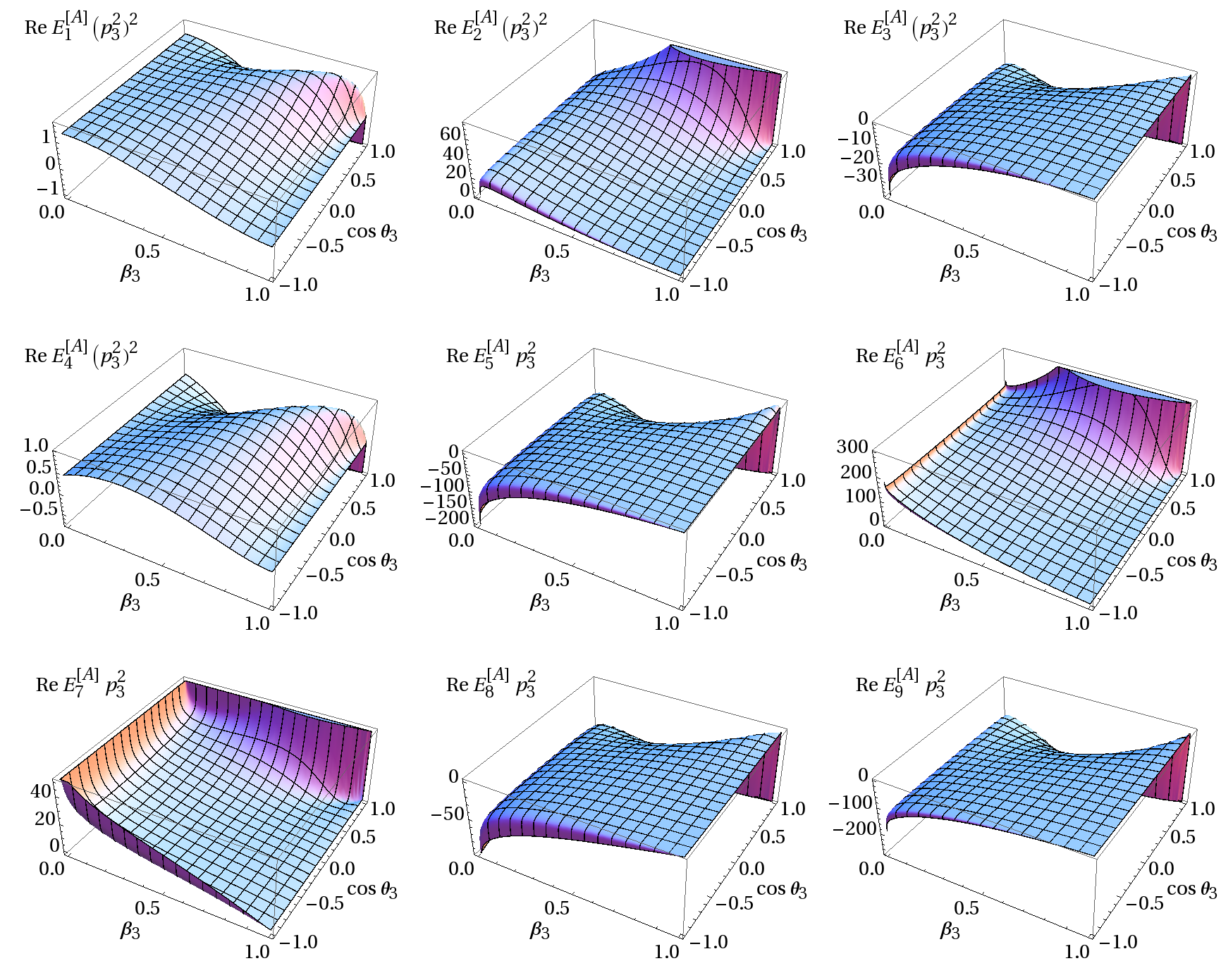
In Figures 2 and 3 we show numerical results for the class and class contributions to our 9 form factors at the two-loop level. Note that these results were obtained with our C++ code and thus demonstrate the high numerical reliability of our implementation. We vary the relativistic velocity, , and the cosine of the scattering angle, , of the vector boson . For the virtualities of the vector bosons we have set . All results are for and given in the -scheme. The class contributions in Figure 2 show pronounced structures in the collinear regions (see (53) for the corresponding tree level coefficients). In contrast, the class contributions in Figure 3 show no such features and are rather smooth functions in the full - plane.
9 Conclusions
In this paper, we presented the derivation of the two-loop massless QCD corrections to the helicity amplitudes for massive vector boson pair production in quark-antiquark annihilation. The combination with leptonic decay currents allows to construct the two-loop QCD matrix elements relevant to four-lepton production. In this course, we computed all master integrals and optimised their representation for numerical performance. Our results obtained for the amplitudes provide a fully independent validation of a recent calculation [32]. We implemented our amplitudes in a C++ code for the fast and stable numerical evaluation of the amplitudes, which we provide together with our analytical results for public access at http://vvamp.hepforge.org. This opens up the path towards precision phenomenology in gauge boson pair production and improvements of the background predictions for Higgs boson studies and searches for physics beyond the Standard Model.
Acknowledgements
We are grateful to K. Melnikov and F. Caola for their help in checking our results against [32]. LT wishes to thank K. Melnikov for a clarifying discussion on the use of 4-dimensional Schouten identities for simplifications of spinor structures. This research was supported in part by the Swiss National Science Foundation (SNF) under contract 200020-149517 and by the Research Executive Agency (REA) of the European Union under the Grant Agreement PITN–GA–2012–316704 (HiggsTools), and the ERC Advanced Grant MC@NNLO (340983). We thank the HepForge team for providing web space for our project. The Feynman graphs in this article have been drawn with JaxoDraw [75, 76].
Appendix A Squared amplitudes for the on-shell production of vector-boson pairs
In this Section we show how the general results described in this article can be used to obtain the squared amplitude for the process summed over spins and colours. For the calculations of the NNLO QCD corrections to on-shell [27] and production [28] production, we directly computed the squared amplitudes using a dedicated setup based on our solutions for the equal-mass master integrals [25, 26]. We compared the results obtained in the two approaches and find full agreement.
We denote the squared amplitude as
| (82) |
which of course can be perturbatively expanded in powers of as
| (83) |
where we have
| (84) | ||||
| (85) | ||||
| (86) |
It is easy to write a general expression of in terms of the coefficients and or, equivalently, in terms of the and , simply by contracting the general decomposition (11) with itself and summing over colours and external polarisations using (9). The result is quite involved and not particularly illuminating and we decided not to include it here explicitly. This general formula, in fact, is needed explicitly only in order to derive the -loop-loop corrections , which can however also be easily extracted from automated codes, and therefore we will not consider them here. On the other hand, if we limit ourselves to considering the contraction of the generic -loop amplitude with the tree-level, i.e. , the results are much more compact. In the following two sections we will discuss the two explicit cases of on-shell and production, which were used for the calculations in [27, 28].
A.1 The two-loop corrections to production
In the case of the tree-level is given by the two diagrams belonging to classes . As far as two-loop corrections are concerned, the classes of diagrams that can contribute to production are , see Section 4. By contracting the tree-level diagrams with the general amplitude (11) one easily finds
| (87) |
where is the number of colours, while and are defined in (34). Each of the can be obtained summing over the relevant classes of diagrams, re-weighted by appropriate coupling factors
| (88) |
where the components of the are defined by a decomposition completely analogous to that for the in (40),
| (89) |
and is defined in (41) . We have verified explicitly that as far at the tree-level and one-loop corrections are concerned, we have full agreement with the results in [69]. Similar but much more lengthy formulas can be derived for , and we do not report them here for brevity.
A.2 The two-loop corrections to production
Let us consider now the case of , where the index labels the flavour of the initial state quarks, . At the tree-level, this process receives contributions from three diagrams, one in class and the other two in class , with . Let us start from the tree-level and one-loop corrections, where only diagrams in classes can contribute. Following the notation of [70], we separate the contributions to the squared amplitude into three different form factors
| (90) |
| (91) |
contains the squared contribution of diagrams in class (i.e. diagrams where the production of the pair is not mediated through a or a boson). encapsulates instead the interference of the -type diagrams (i.e. those where the pair is produced via a or a virtual boson) with diagrams in class . Finally is given by the interference of the -type diagrams with themselves. Again, following closely [70] we define then
| (92) |
where, as always, is the quark charge in units of , with , and the electroweak couplings , and are defined in (34) and (43).
At two loops the decomposition (91) must be enlarged since also diagrams belonging to class start contributing to the amplitude. We therefore write the two-loop contribution as follows
| (93) |
where we introduced the new couplings
| (94) |
Here, the new form factors and contain the contribution from the two-loop diagrams in class . In deriving (94) we used the fact that for a fermion loop with an attached -pair we have
| (95) |
where is the number of generations of massless quarks running in the loop. Note that because of the flavour-change induced by the bosons, we limit ourselves to consider at most massless quarks , i.e. two generations . Finally, the form factor receives contributions only from one class of diagrams, .
At tree level we find that the different form factors can be obtained from
| (96) | ||||
| (97) | ||||
| (98) |
At one loop and two loops we find instead
| (99) |
and the two new form factors read
| (100) | ||||
| (101) |
where are the -loop QCD corrections to the quark form factor. We have verified that the tree-level and one-loop corrections, in the limit of equal virtualities of the massive vector bosons, agree with [70].
Appendix B Schouten identities for the amplitude
In this Appendix, we show how to reduce the number of independent form factors entering our helicity amplitudes by exploiting the 4-dimensionality of external states via Schouten identities. We document here a general way to derive such Schouten identities for the case. The case proceeds in exactly the same way.
We start off by fixing the helicities for a right-handed incoming quark current in the spinor helicity notation and we get
As a first step we notice that we can collect as an overall factor:
Multiplying and dividing by this allows to write the partonic amplitude as
| (102) |
such that every spinor structure is a trace. We can then perform the traces recalling that the transversality of the leptonic decay currents allows to discard contributions proportional to or . In this way we get
| (103) |
and
| (104) |
| (105) |
where we introduced the Levi-Civita tensor, with the following notation
Moreover, note that the asymmetry between (104) and (105) is due to the transversality condition which effectively replaces and .
Using (103),(104) and (105) we see that all spinor structures can be written in terms of the following 11 structures:
This does not appear to be any improvement with respect to the 10 structured we had before. It is nevertheless very easy to show that out of these structures can indeed be expressed as linear combinations of the remaining by means of an anti-symmetrisation of the tensors.
In order to see how this works in practice, we start off by considering . By anti-symmetrising in dimensions one easily finds
| (106) |
which implies that can be eliminated by
| (107) |
leaving us again with structures. One more anti-symmetrisation can be used, namely consider , where the momentum is defined as
such that . Proceeding as before we find
| (108) |
It becomes clear that using these two relations we can eliminate completely and in favour of the remaining structures. In particular these relations can be rephrased in terms of the original spinors in (102) giving two Schouten identities for the spinor lines:
| (109) |
| (110) |
The corresponding relations for the spinors of the left-handed partonic currents can be found by simply permuting . Using (109),(110), and the corresponding ones for the left-handed partonic current, we eliminate of the structures in (102) in favour of , plus the remaining structures, and then proceed by contracting with the left-handed leptonic decay currents (26). As a result one easily arrives at formulae (37) and (38).
Appendix C Conversion to Catani’s original IR subtraction scheme
In Section 6 we derived the finite remainder of the one- and two-loop helicity amplitude coefficients in a subtraction scheme which is particularly well-suited for subtraction [68]. In this Appendix we show how these results can be converted to Catani’s original scheme [67]. Starting from the UV-renormalised coefficients defined in (75) at renormalisation scale , we write the finite remainders in Catani’s scheme as
| (111) |
where Catani’s subtraction operators are defined as
| (112) |
with
| (113) |
and since a pair is the only coloured state we have
| (114) |
In this article, we present our results for . Note that upon expansion in both and generate imaginary parts whose sign is fixed by the prescription .
By comparing (76) with (111) one can show that the parts of the finite, complex form factors in Catani’s original scheme [67], can be obtained from those in the -scheme [68] according to
| (115) |
with the finite scheme conversion coefficients given by
| (116) | ||||
| (117) |
where we have set to match the convention for our final results. Notice that, in order to obtain the finite remainders of the two-loop amplitudes in the two different schemes, only the finite pieces of the latter are required, and in particular the terms of the one-loop amplitudes are not needed, as expected. Note, moreover, that the conversion coefficients are complex, due to the fact that the original formulation of IR subtraction [67] factored out a phase for time-like pairs of partons from both the collinear and soft contributions, while in the -scheme [68] this phase factor is associated only with the soft contributions, in line with the structure of IR factorisation [77, 78] at higher loop order.
References
- (1) J. Ohnemus, Order calculations of hadronic and production, Phys.Rev. D47 (1993) 940–955.
- (2) U. Baur, T. Han, and J. Ohnemus, QCD corrections to hadronic production with nonstandard couplings, Phys.Rev. D48 (1993) 5140–5161, [hep-ph/9305314].
- (3) U. Baur, T. Han, and J. Ohnemus, QCD corrections and anomalous couplings in production at hadron colliders, Phys.Rev. D57 (1998) 2823–2836, [hep-ph/9710416].
- (4) L. J. Dixon, Z. Kunszt, and A. Signer, Helicity amplitudes for O() production of , , , , or pairs at hadron colliders, Nucl.Phys. B531 (1998) 3–23, [hep-ph/9803250].
- (5) J. M. Campbell and R. K. Ellis, An Update on vector boson pair production at hadron colliders, Phys.Rev. D60 (1999) 113006, [hep-ph/9905386].
- (6) L. J. Dixon, Z. Kunszt, and A. Signer, Vector boson pair production in hadronic collisions at order : Lepton correlations and anomalous couplings, Phys.Rev. D60 (1999) 114037, [hep-ph/9907305].
- (7) E. Accomando, A. Denner, and A. Kaiser, Logarithmic electroweak corrections to gauge-boson pair production at the LHC, Nucl.Phys. B706 (2005) 325–371, [hep-ph/0409247].
- (8) E. Accomando and A. Kaiser, Electroweak corrections and anomalous triple gauge-boson couplings in and production at the LHC, Phys.Rev. D73 (2006) 093006, [hep-ph/0511088].
- (9) E. Accomando, A. Denner, and C. Meier, Electroweak corrections to and production at the LHC, Eur.Phys.J. C47 (2006) 125–146, [hep-ph/0509234].
- (10) A. Bierweiler, T. Kasprzik, and J. H. Kuhn, Vector-boson pair production at the LHC to accuracy, JHEP 1312 (2013) 071, [arXiv:1305.5402].
- (11) J. Baglio, L. D. Ninh, and M. M. Weber, Massive gauge boson pair production at the LHC: a next-to-leading order story, Phys.Rev. D88 (2013) 113005, [arXiv:1307.4331].
- (12) M. Billoni, S. Dittmaier, B. Jäger, and C. Speckner, Next-to-leading order electroweak corrections to pp W+W- 4 leptons at the LHC in double-pole approximation, JHEP 1312 (2013) 043, [arXiv:1310.1564].
- (13) S. Gieseke, T. Kasprzik, and J. H. Kühn, Vector-boson pair production and electroweak corrections in HERWIG++, Eur.Phys.J. C74 (2014), no. 8 2988, [arXiv:1401.3964].
- (14) A. Denner, S. Dittmaier, M. Hecht, and C. Pasold, NLO QCD and electroweak corrections to production with leptonic W-boson decays, JHEP 04 (2015) 018, [arXiv:1412.7421].
- (15) C. Anastasiou, K. Melnikov, and F. Petriello, Fully differential Higgs boson production and the di-photon signal through next-to-next-to-leading order, Nucl.Phys. B724 (2005) 197–246, [hep-ph/0501130].
- (16) S. Catani and M. Grazzini, An NNLO subtraction formalism in hadron collisions and its application to Higgs boson production at the LHC, Phys.Rev.Lett. 98 (2007) 222002, [hep-ph/0703012].
- (17) K. Melnikov and F. Petriello, Electroweak gauge boson production at hadron colliders through O(), Phys.Rev. D74 (2006) 114017, [hep-ph/0609070].
- (18) S. Catani, L. Cieri, G. Ferrera, D. de Florian, and M. Grazzini, Vector boson production at hadron colliders: a fully exclusive QCD calculation at NNLO, Phys.Rev.Lett. 103 (2009) 082001, [arXiv:0903.2120].
- (19) Z. Bern, A. De Freitas, and L. J. Dixon, Two loop amplitudes for gluon fusion into two photons, JHEP 0109 (2001) 037, [hep-ph/0109078].
- (20) C. Anastasiou, E. W. N. Glover, and M. Tejeda-Yeomans, Two loop QED and QCD corrections to massless fermion boson scattering, Nucl.Phys. B629 (2002) 255–289, [hep-ph/0201274].
- (21) T. Gehrmann and L. Tancredi, Two-loop QCD helicity amplitudes for and , JHEP 1202 (2012) 004, [arXiv:1112.1531].
- (22) T. Gehrmann, L. Tancredi, and E. Weihs, Two-loop QCD helicity amplitudes for and , JHEP 1304 (2013) 101, [arXiv:1302.2630].
- (23) S. Catani, L. Cieri, D. de Florian, G. Ferrera, and M. Grazzini, Diphoton production at hadron colliders: a fully-differential QCD calculation at NNLO, Phys.Rev.Lett. 108 (2012) 072001, [arXiv:1110.2375].
- (24) M. Grazzini, S. Kallweit, D. Rathlev, and A. Torre, production at hadron colliders in NNLO QCD, Phys.Lett. B731 (2014) 204, [arXiv:1309.7000].
- (25) T. Gehrmann, L. Tancredi, and E. Weihs, Two-loop master integrals for : the planar topologies, JHEP 1308 (2013) 070, [arXiv:1306.6344].
- (26) T. Gehrmann, A. von Manteuffel, L. Tancredi, and E. Weihs, The two-loop master integrals for , JHEP 1406 (2014) 032, [arXiv:1404.4853].
- (27) F. Cascioli, T. Gehrmann, M. Grazzini, S. Kallweit, P. Maierhöfer, et al., ZZ production at hadron colliders in NNLO QCD, Phys.Lett. B735 (2014) 311–313, [arXiv:1405.2219].
- (28) T. Gehrmann, M. Grazzini, S. Kallweit, P. Maierhöfer, A. von Manteuffel, et al., Production at Hadron Colliders in Next to Next to Leading Order QCD, Phys.Rev.Lett. 113 (2014) 212001, [arXiv:1408.5243].
- (29) J. M. Henn, K. Melnikov, and V. A. Smirnov, Two-loop planar master integrals for the production of off-shell vector bosons in hadron collisions, JHEP 1405 (2014) 090, [arXiv:1402.7078].
- (30) F. Caola, J. M. Henn, K. Melnikov, and V. A. Smirnov, Non-planar master integrals for the production of two off-shell vector bosons in collisions of massless partons, JHEP 1409 (2014) 043, [arXiv:1404.5590v2].
- (31) C. G. Papadopoulos, D. Tommasini, and C. Wever, Two-loop Master Integrals with the Simplified Differential Equations approach, JHEP 1501 (2015) 072, [arXiv:1409.6114].
- (32) F. Caola, J. M. Henn, K. Melnikov, A. V. Smirnov, and V. A. Smirnov, Two-loop helicity amplitudes for the production of two off-shell electroweak bosons in quark-antiquark collisions, JHEP 1411 (2014) 041, [arXiv:1408.6409].
- (33) F. Chavez and C. Duhr, Three-mass triangle integrals and single-valued polylogarithms, JHEP 1211 (2012) 114, [arXiv:1209.2722].
- (34) C. Anastasiou, J. Cancino, F. Chavez, C. Duhr, A. Lazopoulos, et al., NNLO QCD corrections to pp in the large NF limit, JHEP 1502 (2015) 182, [arXiv:1408.4546].
- (35) A. Denner and T. Sack, Electroweak radiative corrections to , Nucl.Phys. B306 (1988) 221.
- (36) K. Diener, B. A. Kniehl, and A. Pilaftsis, Loop effects of exotic leptons on vector boson pair production at colliders, Phys.Rev. D57 (1998) 2771–2784, [hep-ph/9709361].
- (37) A. Denner, Techniques for calculation of electroweak radiative corrections at the one loop level and results for W physics at LEP-200, Fortsch.Phys. 41 (1993) 307–420, [arXiv:0709.1075].
- (38) L. J. Dixon, Calculating scattering amplitudes efficiently, hep-ph/9601359.
- (39) E. W. N. Glover and J. van der Bij, Z Boson Pair Production via Gluon Fusion, Nucl.Phys. B321 (1989) 561.
- (40) E. N. Glover and J. van der Bij, Vector Boson Pair Production via Gluon Fusion, Phys.Lett. B219 (1989) 488.
- (41) K. Melnikov and M. Dowling, Production of two Z-bosons in gluon fusion in the heavy top quark approximation, Phys. Lett. B744 (2015) 43–47, [arXiv:1503.01274].
- (42) T. Gehrmann, T. Huber, and D. Maitre, Two-loop quark and gluon form-factors in dimensional regularisation, Phys.Lett. B622 (2005) 295–302, [hep-ph/0507061].
- (43) P. Nogueira, Automatic Feynman graph generation, J.Comput.Phys. 105 (1993) 279–289.
- (44) A. von Manteuffel and C. Studerus, Reduze 2 - Distributed Feynman Integral Reduction, arXiv:1201.4330.
- (45) C. Studerus, Reduze-Feynman Integral Reduction in C++, Comput.Phys.Commun. 181 (2010) 1293–1300, [arXiv:0912.2546].
- (46) C. W. Bauer, A. Frink, and R. Kreckel, Introduction to the GiNaC framework for symbolic computation within the C++ programming language, J.Symb.Comput. 33 (2002) 1–12, [cs/0004015].
- (47) R. Lewis, Computer Algebra System Fermat. http://www.bway.net/~lewis.
- (48) F. Tkachov, A Theorem on Analytical Calculability of Four Loop Renormalization Group Functions, Phys.Lett. B100 (1981) 65–68.
- (49) K. Chetyrkin and F. Tkachov, Integration by Parts: The Algorithm to Calculate beta Functions in 4 Loops, Nucl.Phys. B192 (1981) 159–204.
- (50) T. Gehrmann and E. Remiddi, Differential equations for two loop four point functions, Nucl.Phys. B580 (2000) 485–518, [hep-ph/9912329].
- (51) S. Laporta, High precision calculation of multiloop Feynman integrals by difference equations, Int.J.Mod.Phys. A15 (2000) 5087–5159, [hep-ph/0102033].
- (52) J. Vermaseren, New features of FORM, math-ph/0010025.
- (53) A. Kotikov, Differential equations method: New technique for massive Feynman diagrams calculation, Phys.Lett. B254 (1991) 158–164.
- (54) E. Remiddi, Differential equations for Feynman graph amplitudes, Nuovo Cim. A110 (1997) 1435–1452, [hep-th/9711188].
- (55) M. Caffo, H. Czyz, S. Laporta, and E. Remiddi, The Master differential equations for the two loop sunrise selfmass amplitudes, Nuovo Cim. A111 (1998) 365–389, [hep-th/9805118].
- (56) C. Duhr, Hopf algebras, coproducts and symbols: an application to Higgs boson amplitudes, JHEP 1208 (2012) 043, [arXiv:1203.0454].
- (57) R. Bonciani, A. Ferroglia, T. Gehrmann, A. von Manteuffel, and C. Studerus, Light-quark two-loop corrections to heavy-quark pair production in the gluon fusion channel, JHEP 1312 (2013) 038, [arXiv:1309.4450].
- (58) J. M. Henn, Multiloop integrals in dimensional regularization made simple, Phys.Rev.Lett. 110 (2013) 251601, [arXiv:1304.1806].
- (59) A. Kotikov, The Property of maximal transcendentality in the N=4 Supersymmetric Yang-Mills, arXiv:1005.5029.
- (60) J. Vollinga and S. Weinzierl, Numerical evaluation of multiple polylogarithms, Comput.Phys.Commun. 167 (2005) 177, [hep-ph/0410259].
- (61) A. Goncharov, Multiple polylogarithms and mixed Tate motives, math/0103059.
- (62) F. Brown, The Massless higher-loop two-point function, Commun.Math.Phys. 287 (2009) 925–958, [arXiv:0804.1660].
- (63) A. B. Goncharov, M. Spradlin, C. Vergu, and A. Volovich, Classical Polylogarithms for Amplitudes and Wilson Loops, Phys.Rev.Lett. 105 (2010) 151605, [arXiv:1006.5703].
- (64) C. Duhr, H. Gangl, and J. R. Rhodes, From polygons and symbols to polylogarithmic functions, JHEP 1210 (2012) 075, [arXiv:1110.0458].
- (65) C. Duhr, Mathematical aspects of scattering amplitudes, arXiv:1411.7538.
- (66) A. von Manteuffel, R. M. Schabinger, and H. X. Zhu, The Complete Two-Loop Integrated Jet Thrust Distribution In Soft-Collinear Effective Theory, JHEP 1403 (2014) 139, [arXiv:1309.3560].
- (67) S. Catani, The Singular behavior of QCD amplitudes at two loop order, Phys.Lett. B427 (1998) 161–171, [hep-ph/9802439].
- (68) S. Catani, L. Cieri, D. de Florian, G. Ferrera, and M. Grazzini, Universality of transverse-momentum resummation and hard factors at the NNLO, Nucl.Phys. B881 (2014) 414–443, [arXiv:1311.1654].
- (69) B. Mele, P. Nason, and G. Ridolfi, QCD radiative corrections to Z boson pair production in hadronic collisions, Nucl.Phys. B357 (1991) 409–438.
- (70) S. Frixione, A Next-to-leading order calculation of the cross-section for the production of W+ W- pairs in hadronic collisions, Nucl.Phys. B410 (1993) 280–324.
- (71) F. Cascioli, P. Maierhofer, and S. Pozzorini, Scattering Amplitudes with Open Loops, Phys.Rev.Lett. 108 (2012) 111601, [arXiv:1111.5206].
- (72) G. Chachamis, M. Czakon, and D. Eiras, W Pair Production at the LHC. I. Two-loop Corrections in the High Energy Limit, JHEP 0812 (2008) 003, [arXiv:0802.4028].
- (73) D. Maître and P. Mastrolia, S@M, a Mathematica Implementation of the Spinor-Helicity Formalism, Comput. Phys. Commun. 179 (2008) 501–574, [arXiv:0710.5559].
- (74) B. Haible and R. B. Kreckel, CLN: Class Library for Numbers. http://www.ginac.de/CLN.
- (75) D. Binosi and L. Theussl, JaxoDraw: A Graphical user interface for drawing Feynman diagrams, Comput.Phys.Commun. 161 (2004) 76–86, [hep-ph/0309015].
- (76) J. Vermaseren, Axodraw, Comput.Phys.Commun. 83 (1994) 45–58.
- (77) E. Gardi and L. Magnea, Factorization constraints for soft anomalous dimensions in QCD scattering amplitudes, JHEP 0903 (2009) 079, [arXiv:0901.1091].
- (78) T. Becher and M. Neubert, On the Structure of Infrared Singularities of Gauge-Theory Amplitudes, JHEP 0906 (2009) 081, [arXiv:0903.1126].