Cosmological inflation in gravity
Abstract
Cosmological inflation is discussed in the framework of gravity where is a generic function of the curvature scalar and the Gauss-Bonnet topological invariant . The main feature that emerges in this analysis is the fact that this kind of theory can exhaust all the curvature budget related to curvature invariants without considering derivatives of , etc. in the action. Cosmological dynamics results driven by two effective masses (lenghts) related to the scalaron and the scalaron working respectively at early and very early epochs of cosmic evolution. In this sense, a double inflationary scenario naturally emerges.
Keywords:
Cosmology; dark energy; alternative gravity theories; topological invariant; exact solutions.pacs
98.80.-k, 95.35.+d, 95.36.+xI Introduction
Inflationary paradigm was introduced to address problems and shortcomings related to the self-consistency of the Cosmological Standard Model at early stages of its evolution [1, 2, 3, 4, 5]. The inflationary mechanism can be achieved in several different ways considering primordial scalar fields or geometric corrections into the effective gravitational action. The general aim is to address problems like the initial singularity, the cosmological horizon, the cosmic microwave background isotropy (and the related anisotropies generated, in principle, with initial quantum fluctuations), the large scale structure formation and evolution, the absence of magnetic monopoles and so on [6, 7, 8, 9, 10]. The main ingredient of all these scenarios is to claim that an inflationary phase occurs at some stage in the early universe and that one or more sources, different from standard ordinary matter, give rise to accelerated cosmic expansion. Such an expansion can be a single or a multiple event often related to the formation of structure at large and at very large scale. In general, inflationary scenarios originated from some fundamental theory like quantum gravity, strings, M-theory or GUT models. Reversing the argument, inflationary models and observables related to inflation can be used to probe fundamental theories (see, for example the latest results of the PLANCK and BICEP2 collaborations [12, 13, 11]).
In particular, quantum fluctuations of a given scalar field i.e. the inflaton, gives a mechanism for the origin of large scale structure. In other words, inflation gives rise to density perturbations that exhibit a scale invariant spectrum. Such a feature, in principle, is directly observed by measuring the temperature anisotropies in cosmic microwave background [13, 15, 16, 17, 18, 19]. A part the general features, the possibilities to realize inflation are several. For example, in the old inflation, inflaton is trapped in a false vacuum phase through a first order transition, while, in the new inflation, expansion ends up with a second order phase transition after a slow rolling phase [2, 3, 4]. According to the problems to address, there are several different inflationary models, for example the power law inflation, the hybrid inflation, the oscillating inflation, the trace-anomaly driven inflation, the -inflation, the ghost-inflation, the tachyon inflation and so on [20, 21, 22, 23, 24, 25, 26]. Furthermore, some of these models have no potential minimum and the inflationary mechanism appears different with respect to the standard one. See for example the quintessential inflation [27] or the tachyon inflation [28, 29, 30, 31, 32, 33].
A natural way to achieve inflation is considering higher-order curvature corrections in the Hilbert-Einstein Lagrangian [34, 35, 36, 37, 38, 39, 40, 41, 42, 43, 44]. The first and well-known example of this approach is the Starobinsky model [1] where inflation is essentially driven by contributions, being the Ricci curvature scalar. After this preliminary model, other higher-order curvature terms have been taken into account [45, 47, 46, 48, 49, 50, 51, 52]. The philosophy is that, in the early higher-curvature regime, such further curvature invariants come out as renormalization terms in quantum field theories in curved spacetime [53]. Furthermore, under conformal transformations, the theory becomes minimally coupled in the Einstein frame. In this frame, the conformal scalar field assumes the role of inflaton and leads the primordial acceleration [52]. However, more than one scalar field can be achieved by conformal transformations disentangling the degrees of freedom present in the Jordan frame.
Several combinations of curvature invariants, like can be considered [54, 55, 57, 58]. The goal is to explain both the early and the late-time acceleration in a geometrical way [60] without invoking huge amount of dark energy or, sometime, ill-defined scalar fields. Among these attempt, a key role is played by the Gauss-Bonnet topological invariant that naturally arises in the process of quantum field theory regularization and renormalization in curved spacetime [53]. In particular, it contributes to the trace anomaly where higher-order curvature terms are present [72]. In some sense, considering a theory where both and are nonlinearly present exhausts the budget of curvature degrees of freedom needed to extend General Relativity since the Ricci scalar and both the Ricci and the Riemann tensors are present in the definition of . From the inflation point of view, introducing beside gives the opportunity to achieve a double inflationary scenario where the two acceleration phases are led by and respectively. As we will see below, this happens as soon as both and appear in non-linear combinations since linear means just General Relativity (and then no inflation) and linear identically vanishes in 4D gravitational action, being an invariant. On the other hand, the combination of both terms seems to improve the inflationary mechanism since one achieves a -dominated phase and a -dominated phase. The second leads the Universe at very early stages of its evolution because is quadratic in curvature invariants and then it is dominant in stronger curvature regimes. Specifically, using a non linear function of , inserted into the approach, that is a function, extends the Starobinsky model since the whole curvature "interactions", present in the early Universe, are taken into account. In view of the recent results by the PLANCK [11] and BICEP2 [12] collaborations, the potential advantages of this class of models, with respect to the original Starobinsky one, could be that curvature degrees of freedom (in particular the scalaron ) result better constrained (see [13] for a detailed discussion). A first study in this sense is in the paper by Ivanov and Toporensky [14], where cosmological dynamics of fourth order gravity is studied in presence of Gauss-Bonnet term.
In this paper, we discuss the possibility to obtain inflation considering a generic theory where, in principle, both and are non linear in the action. There are several recent studies on models of this type [61, 62, 63, 67, 68, 69, 70, 71]. All of them, put in evidence the fact that the Gauss-Bonnet topological invariant can solve some shortcomings of the original gravity and contributes, in non trivial way, to the accelerated expansion.
The paper is organized as follows. In Sec. II, we derive the field equations for . General features of cosmology and inflation are discussed in Sec. III. Sec IV is devoted to the discussion of exact solutions coming from Noether symmetries giving rise to power-law inflation. Summary and outlook are given in Sec. V.
II Field equations of -gravity
Let us start by writing the most general action for modified Gauss-Bonnet gravity
| (1) |
where, as we said before, is a function of the Ricci scalar and Gauss-Bonnet invariant defined as
| (2) |
Moreover , with Newton constant. We are using physical units . We are discarding, for the moment, the contribution of standard matter Lagrangian that we will reconsider below. The variation of the action (1) with respect to the metric provides the following gravitational field equations [68]
| (3) |
The trace is
| (4) |
where is the d’Alembert operator in curved spacetime and
| (5) |
are the partial derivatives with respect to and . It is possible to define two different potentials that depend on the scalar curvature and the Gauss-Bonnet invariant that enter the trace equation with their partial derivatives
| (6) | |||
| (7) |
It is important to emphasize that, from Eqs.(3)-(4), General Relativity is recovered as soon as . Furthermore, if is not considered, we are exactly in the gravity context. Clearly, as in the case of the Starobinsky scalaron, plays the role of a further scalar field whose dynamics is given by the Klein-Gordon-like Eq. (4). This means that we can expect a natural double inflation where both geometric fields play a role. As for the scalaron, we can expect a mass for the scalaron which determine the "strength" of the -dominated inflation.
III double inflation
Let us consider now a flat Friedman-Robertson-Walker (FRW) metric
| (8) |
where is the scale factor of the Universe. Inserting this metric into the action (1) and assuming suitable Lagrange multipliers for and , we obtain the point-like Lagrangian [67]
| (9) |
which is a canonical function depending on and defined in the configuration space . Specifically, the Lagrangian (9) has a canonical form thanks to the Lagrange multipliers
| (10) |
| (11) |
that are also field equations for the related dynamical system [67]. Here is the Hubble parameter and the overdot denotes the derivative with respect to the cosmic time . The cosmological equations in term of , are
| (12) | |||
where Eq. (12) is the energy condition, that is the Einstein equation. The full dynamical system of cosmology is given by Eqs. (10), (11), (12), (12).
To obtain inflation, the following conditions have to be satisfied:
| (14) |
It means, that the magnitude of the slow-roll parameters
| (15) |
has to be small during inflation. Moreover, is necessary to have . The acceleration is expressed as
| (16) |
and then the accelerated expansion ends only when the slow-roll parameter is of the unit order.
In order to discuss a possible inflationary scenario, let us choose, for example, the following Lagrangian
| (17) |
where and are constants of the dimension length squared and length to the fourth power respectively. The linear term in is included to produce the correct weak-field limit. It is easy to see that we have considered a model with a correction which adds new degrees of freedom due to the presence of the Gauss-Bonnet term. In the above Lagrangian, the term is the first significant term in since the linear one gives no contribution11 1 In four dimensions, we have (18) This means that only a function of the Gauss-Bonnet invariant makes this integral non-trivial. On the other hand, in five or higher dimensions Eq.(18) is different from zero. . As it is well known, a theory like is capable of producing an inflationary scenario [1] not excluded from the last PLANCK release [11].
Here we concentrate on the question if such an inflationary scenario can be improved considering the whole curvature budget that can be encompassed by adding a non linear function of the Gauss-Bonnet invariant. In such a case, as stressed above, we can have a -driven inflation led by the term and a -driven inflation led by term. However, this is nothing else but a toy model that should be improved by realistic forms of the function.
To develop our considerations, let us consider the point-like Lagrangian (9). It is well known that, in analytical mechanics, any Lagrangian can be decomposed as
| (19) |
where and are the kinetic energy and potential energy respectively. Here we have and . In the case of Lagrangian (9), considering the Lagrangian density, i.e. , it is
| (21) |
Assuming the model (17), we have
| (22) | |||||
In Fig. 1, a qualitative shape of the potential is reported. A possible slow-roll trajectory is shown.
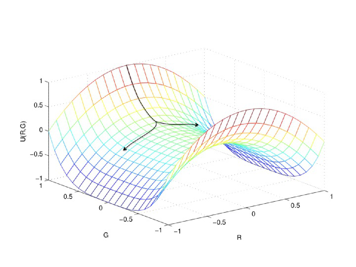

It is important to stress the effective behavior of the Lagrangian (17) that assumes the following form
| (23) |
In other words, the correction to the model due to the presence of topological term can be seen as a sort of correction. However, it is important to stress that and have roughly the same dynamical role only at background level for the homogeneous and isotropic FRW metric. As soon as one takes into account anisotropies and inhomogeneities, and assume different roles since extra diagonal components of the Ricci and Riemann tensors cannot be discarded. In other words, considering the definition of the Gauss-Bonnet invariant, given in Eq.(2), only in the FRW context. If more general situations are assumed, this approximation no longer holds. This means that and can be observationally distinguished only evaluating anisotropies and inhomogeneities resulting from perturbations where extra diagonal components of the Ricci and Riemann tensors are not negligible.
In Fig. 2, the trends of sections are reported according to the dominance of the terms in the potential.
Let us describe now the qualitative evolution of the model. The behavior is different depending on the "strength" of or terms. In fact, they give rise to a potential with two minima that can be separated by a barrier (see Fig. 2 in the bottom). This represent a double inflationary scenario where -scalar dominates at early epochs, at moderate early epochs dominate -scalar and finally the model converges towards standard General Relativity. Due to the fact that runs as , it is dominant at very high curvature improving, in some sense, the Starobinsky inflation. In the present simple toy-model, we considered and this means, as pointed out above, that . From the energy condition, given by Eq. (12), we have
| (24) | |||
and from (12), we obtain
Considering the slow-roll conditions and , this implies that . From Eq.(24), one has
| (26) |
In order to study the evolution of the model, we have to distinguish among the various regimes. Let us suppose that
| (27) |
Then Eq. (26) takes the form
| (28) |
and we obtain that
| (29) |
and the solution for the scale factor is
| (30) |
This is nothing else but the well known inflation where the sign and the value of determine the number of e-foldings [59].
On the other hand we can consider the regime
| (31) |
where
| (32) |
Inflation is recovered for
| (33) |
and then it is
| (34) |
From the above considerations, we can introduce a further mass term
| (35) |
due to the Gauss-Bonnet correction that leads another earlier inflationary behavior. In conclusion, it seems that considering the whole curvature budget in the effective action (i.e. the further combinations of curvature invariants more than the linear ) means to introduce two effective masses that lead the dynamics. It is important to stress that the parameters and have to be consistent with the Solar System constraints according to the chameleon mechanism. Clearly, in the low energy regime, General Relativity has to be recovered and then the quadratic and quartic terms in must be negligible. Essentially, starting from very early epochs, one has first to recover the Starobinsky model and then the Einstein regime. This means that the two-scalaron regimes, leading the two early inflationary phases, have to become negligible for to recover the standard Newtonian potential. In such a case, an analysis like that in [64, 65] leads to assume the values of the parameters and of the order unit to achieve the consistency with the chameleon mechanism and the Solar System experiments.
IV power-law Inflation
Also power-law inflation can be easily achieved in the framework of gravity. In particular, using the Noether Symmetry Approach [66] in the generic action (1) and choosing appropriate Lagrangian multipliers that make the point-like Lagrangian canonical, models where conserved quantities emerge can be selected (see also [73, 76, 74, 75, 77, 78] for analogue cases). This means to impose
| (36) |
where is the Lie derivative with respect to the Noether vector acting on the point-like Lagrangian . A possible choice is to consider the class of Lagrangians
| (37) |
related to the presence of the Noether symmetries [67]. For , it is Inserting this choice into the point-like Lagrangian (9), it becomes,
| (38) | |||||
The same choice can be done into the cosmological Eqs. (12) and (12) that are nothing else but the Euler-Lagrange equations of the Lagrangian (38) together with the Lagrange multipliers (10) and (11). Power law solutions for (38) are easily found [67, 69]. For example we have
| (39) |
A further interesting solution is
| (40) |
General conditions between the exponents and are:
| (41) |
In one these conditions the two constraint are satisfied and are of the same form. It is easy to verify that solutions (39) and (40) are in one of these cases.
In order to discuss inflation, we have to consider Eqs. (12) and (12). One obtains the following relations
| (42) |
| (43) |
A condition for inflation is
| (44) |
The slow roll conditions are
| (45) |
| (46) |
Considering the relation , slow roll conditions on and are satisfied for . In conclusion, we can easily see that, for relatively large , slow-roll conditions are satisfied. In Figs. 3 and 4, qualitative pictures of the parameter space regions where inflation is allowed are reported.


Furthermore we can evaluate the anisotropies and the power spectrum coming from inflation using the slow-roll parameters. The spectral index and the tensor-to-scalar ratio are respectively
| (47) |
while the amplitude of the primordial power spectrum is
| (48) |
We obtain that the values and are in good agreement with the observational values of spectral index estimated by PLANCKWP data, i.e. (68 CL) and (95 CL) [13, 11]. These results are consistent also with the values measured by the BICEP2 collaboration [12].
Finally, it is possible to estimate the grow factor for the class of models . Let us consider the equation which governs the evolution of the matter fluctuations in the linear regime
| (49) |
where is the matter density and is the effective Newton coupling which, in our case, is
| (50) |
where is the Newton gravitational constant. However, we are considering perfect fluid matter that enters minimally coupled in action (1). We use Eq. (12) with matter density contribution as follow
| (51) |
with
Inserting Eqs. (50) and (51) into Eq.(49), we obtain the equation
Now, considering relations (41), we have and consequently , therefore, Eq.(IV) becomes
| (54) |
Eq.(54) is an Euler equation whose general solution is
| (55) |

Since we have that
| (56) |
where is the Hubble constant that can be chosen as a prior in agreement with data. The deceleration parameter is
| (57) |
In Fig. 5, the comparison between a model with the CDM analogue is reported.
By a rapid inspection of the figure, it is evident that there is no change in the evolution of the curve since, for any model the deceleration parameter preserves sign, and therefore the universe always accelerates or always decelerates depending on the value of . Clearly, for , the solution is an Einstein-de Sitter model as it has to be. On the other hand, the accelerated expansion of the universe () is recovered for , but, in this case, the universe accelerates forever without the possibility of structure formation. In conclusion, we have to stress that more realistic models are necessary in order to fit the observations.
V Conclusions
In this paper, we have considered the possibility to obtain cosmological inflation starting from a generic function of the Ricci curvature scalar and the Gauss-Bonnet topological invariant . Such a kind of theories, due to the algebraic relation among the curvature invariants in , see Eq. (2), can exhaust the whole curvature budget of effective gravitational theories where derivatives of curvature invariants are not present. The main feature that emerges by this approach is the fact that two effective masses have to be considered, one related to and the other related to . These masses define two different scales that drive dynamics at early and very early epochs, giving rise to a natural double inflationary scenario. Here we have sketched the essential characteristics of this picture considering exponential and power law inflation. However, the theory has to be worked out in order to select reliable models to be compared with data. In a forthcoming paper, the matching with data will be addressed in details.
Acknowledgements
The Authors thank the Referee for the useful comments and hints that allowed to improve the paper. The authors acknowledge INFN Sez. di Napoli (Iniziative Specifiche QGSKY, QNP, and TEONGRAV) for financial support.
References
- [1] A. A. Starobinsky, Phys. Lett. B 91, 99 (1980).
- [2] A. H. Guth, Phys. Rev. D 23, 347 (1981).
- [3] K. Sato, Mon. Not. R. Astron. Soc. 195, 467 (1981).
- [4] K. Sato, Phys. Lett. B 99, 66 (1981).
- [5] D. Kazanas, Astrophys. J. 241, L59 (1980).
- [6] E. W. Kolb and Turner, The Early Universe, Addison-Wesley, Redwood City (1990).
- [7] V. F. Mukhanov and G. V. Chibisov, JETP Lett. 33, 532 (1981);Pisma Zh. Eksp. Teor. Fiz. 33, 549 (1981).
- [8] A. H. Guth and S. Y. Pi, Phys. Rev. Lett. 49, 1110 (1982).
- [9] S. W. Hawking, Phys. Lett. B 115, 295 (1982).
- [10] A. A. Starobinsky, Phys. Lett. B 117, 175 (1982).
- [11] Planck Collaboration, arXiv:1502.02114 [astro-ph.CO] (2015); arXiv:1502.01590 [astro-ph.CO] (2015); arXiv:1502.01589 [astro-ph.CO] (2015).
- [12] BICEP2 Collaboration, Phys. Rev. Lett. 112, 241101 (2014).
- [13] Planck Collaboration, Astron. Astrophys. 571, A22 (2014).
- [14] M. M. Ivanov and A. V. Toporensky, Grav. Cosmol. 18, 43 (2012).
- [15] D. N. Spergel et al., Astrophys. J. Suppl. 148, 175 (2003).
- [16] H. V. Peiris et al., Astrophys. J. Suppl. 148, 213 (2003).
- [17] M. Tegmark et al. [SDSS Collaboration], Phys. Rev. D 69, 103501 (2004).
- [18] M. Tegmark et al. [SDSS Collaboration], Astrophys. J. 606, 702 (2004).
- [19] W. J. Percival et al., Mon. Not. Roy. Astron. Soc. 327, 1297 (2001).
- [20] E. W. Kolb, Pritzker Symposium and Workshop on the Status of Inflationary Cosmology, arXiv:hep-ph/9910311 (1999).
- [21] A. D. Linde, Phys. Lett. B 129 177 (1983).
- [22] A. D. Linde, Phys. Lett. B 108, 389 (1982).
- [23] A. Albrecht and P. Steinhardt, Phys. Rev. Lett. 48, 1220 (1982).
- [24] K. Freese, J. A. Frieman and A. V. Olinto, Phys. Rev. Lett. 65, 3233 (1990).
- [25] D. Polarski and A. A. Starobinsky, Nucl. Phys. B 385, 623 (1992).
- [26] A. D. Linde, Phys. Rev. D 49, 748 (1994).
- [27] P. J. E. Peebles and A. Vilenkin, Phys. Rev. D 59, 063505 (1999).
- [28] M. Fairbairn and M. H. G. Tytgat, Phys. Lett. B 546, 1 (2002).
- [29] A. Feinstein, Phys. Rev. D 66, 063511 (2002).
- [30] T. Padmanabhan, Phys. Rev. D 66, 021301 (2002).
- [31] M. Sami, Mod. Phys. Lett. A 18, 691 (2003).
- [32] M. Sami, P. Chingangbam and T. Qureshi, Phys. Rev. D 66, 043530 (2002).
- [33] S. Thomas and J. Ward, Phys. Rev. D 72, 083519 (2005).
- [34] S. Capozziello, M. De Laurentis, Phys. Rept. 509, 167 (2011).
- [35] S. Nojiri, S. D. Odintsov, Phys. Rept. 505, 59 (2011).
- [36] S. Nojiri, S. D. Odintsov, eConf. C 0602061, 06 (2006).
- [37] S. Nojiri, S. D. Odintsov, Int. J. Geom. Meth. Mod. Phys. 4, 115 (2007).
- [38] S. Capozziello, M. Francaviglia, Gen. Rel. Grav. 40, 357 (2008).
- [39] S. Capozziello, M. De Laurentis, V. Faraoni, The Open Astr. Jour , 2, 1874 (2009).
- [40] A. de la Cruz-Dombriz and D. Saez-Gomez, Entropy 14, 1717 (2012).
- [41] G. J. Olmo, Int. J. Mod. Phys. D 20, 413 (2011).
- [42] F. S. N. Lobo, Dark Energy-Current Advances and Ideas, 173-204 (2009), Research Signpost, ISBN 978-81-308-0341-8arXiv:0807.1640 [gr-qc].
- [43] S. Capozziello and V. Faraoni, Beyond Einstein gravity: A Survey of gravitational theories for cosmology and astrophysics. Fundamental Theories of Physics. 170. Springer. (2010), ISBN 978-94-007-0164-9.
- [44] S. Capozziello and M. De Laurentis, Invariance Principles and Extended Gravity: Theories and Probes, Nova Science Publishers, Inc. (2010) ISBN: 978-1-61668-500-3.
- [45] K. i. Maeda and N. Ohta, Phys. Lett. B 597, 400 (2004).
- [46] S. Nojiri and S. D. Odintsov, Phys. Lett. B 484, 119 (2000).
- [47] S. Nojiri, S. D. Odintsov and S. Zerbini, Phys. Rev. D 62, 064006 (2000).
- [48] S. Nojiri and S. D. Odintsov, Phys. Rev. D 68, 123512 (2003).
- [49] S. W. Hawking, T. Hertog and H. S. Reall, Phys. Rev. D 63, 083504 (2001).
- [50] J. R. Ellis, N. Kaloper, K. A. Olive and J. Yokoyama, Phys. Rev. D 59, 103503 (1999).
- [51] M. C. Bento and O. Bertolami, Phys. Lett. B 228, 348 (1989).
- [52] K. I. Maeda, Phys. Rev. D 39, 3159 (1989).
- [53] N.D. Birrell, P.C.W. Davies, Quantum Fields in Curved Space, Cambridge University Press, Cambridge, UK (1982).
- [54] D. Gorbunov and A. Tokareva, Phys. Lett. B 739, 50 (2014).
- [55] R. Myrzakulov, S. Odintsov and L. Sebastiani, arXiv:1412.1073 [gr-qc], (2014).
- [56] J. D. Barrow and A. C. Ottewill, J. Phys. A: Math. Gen. 16, 2757 (1983).
- [57] K. Bamba, R. Myrzakulov, S. D. Odintsov and L. Sebastiani, Phys. Rev. D 90, 043505 (2014).
- [58] L. Sebastiani, G. Cognola, R. Myrzakulov, S. D. Odintsov and S. Zerbini, Phys. Rev. D 89, 023518 (2014).
- [59] A. Vilenkin, Phys. Rev. D 32 , 2511 (1985).
- [60] S. Capozziello, Int. J. Mod. Phys. D 11, 483 (2002).
- [61] S. Nojiri and S.D. Odintsov, Phys.Lett. B 631, 1 (2005).
- [62] A. De Felice and T. Tanaka, Prog. Theor. Phys. 124, 503 (2010).
- [63] A. De Felice and T. Suyama, JCAP 0906, 034 (2009).
- [64] S. Capozziello and S. Tsujikawa, Phys.Rev. D 77, 107501 (2008).
- [65] Y. Ito and S. Nojiri, Phys.Rev. D 79 103008 (2009).
- [66] S. Capozziello, R. de Ritis, C. Rubano and P. Scudellaro, Riv.Nuovo Cim. 19 (4), 1 (1996).
- [67] S. Capozziello, M. De Laurentis and S. D. Odintsov, Mod. Phys. Lett. A 29, 1450164 (2014).
- [68] M. De Laurentis and A. J. Lopez-Revelles Int. J. Geom. Meth. Mod. Phys. 11, 1450082 (2014).
- [69] M. De Laurentis, Mod. Phys. Lett. A, 30, 1550069 (2015).
- [70] E. Elizalde, R. Myrzakulov, V. V. Obukhov and D. Sáez-Gómez, Class. Quant. Grav. 27, 095007 (2010).
- [71] R. Myrzakulov, D. Sáez-Gómez and A. Tureanu, Gen. Rel. Grav. 43 ,1671 (2011).
- [72] N.H. Barth, S. Christensen, Phys. Rev. D 28, 8 (1983).
- [73] S. Capozziello, M. De Laurenits, Int. J. Geom. Meth. Mod. Phys. 11, 1460004 (2014).
- [74] S. Capozziello, R. de Ritis, and A.A. Marino Class. Quant. Grav. 14, 3259 (1997).
- [75] S. Capozziello, G. Marmo, C. Rubano, and P. Scudellaro Int. J. Mod. Phys. D 6, 491 (1997).
- [76] S. Capozziello and G. Lambiase, Gen.Rel.Grav. 32, 295 (2000).
- [77] S. Capozziello, M. De Laurentis, R. Myrzakulov, arXiv:1412.1471 (2014).
- [78] S. Capozziello, M. De Laurentis, R. Myrzakulov, Int. J. Geom. Methods Mod. Phys. DOI: 10.1142/S0219887815500656, arXiv:1411.7523 (2014).
- [79] S. Basilakos, S. Nesseris, and L. Perivolaropoulos, Phys. Rev. D 87, 123529 (2013).
- [80] S. Basilakos, S. Capozziello, M. De Laurentis, A. Paliathanasis, M. Tsamparlis, Phys.Rev. D 88, 103526 (2013).