Quantum Cloning using Protective Measurement

“ There is no law other than the law that there is no law…All is mutable ”$-$ J A Wheeler [1]. Then how about the ‘no-cloning’ law? Assume there exists a unitary operator $U$ which can clone two non-orthogonal states as follows:

$\displaystyle U|{0}\rangle|{0}\rangle=|{0}\rangle|{0}\rangle,~U|{+}\rangle|{0}\rangle=|{+}\rangle|{+}\rangle$

(1)

where, $|{+}\rangle=(|{0}\rangle+|{1}\rangle)/\sqrt{2}$, and, $\{|{0}\rangle,|{1}\rangle\}$ are eigenkets of $z$-component of total spin angular momentum ($S_{z}$). Now taking the inner product of two equatons in 1, we get $1=\sqrt{2}$, which is wrong. Hence, generalizing, we can say, it is impossible to clone an arbitrary unknown quantum state (which is non-orthogonal to the reference state $|{0}\rangle$, in eq. 1, of course excluding $|{0}\rangle$) via a single unitary operation, which is the essence of no-cloning theorem. Now instead consider the following operation:

	$\displaystyle D|{0}\rangle|{0}\rangle=|{0}\rangle|{0}\rangle,~D|{+}\rangle|{0}\rangle=|{+}\rangle|{+}\rangle,$		(2)
	$\displaystyle D=\sum\limits_{k,l=0}^{3}h_{kl}\sigma_{k}\otimes\sigma_{l}~~~~~~~~~~~~~~$		(3)

where, $D$ is an arbitrary linear operator on the Hilbert space, $\mathcal{H}_{2}\otimes\mathcal{H}_{2}$, of two spin-1/2 particles. Operators $\{\frac{1}{2}\sigma_{k}\otimes\sigma_{l};k,l=0,1,2,3\}$, where, $\sigma_{0}=\mathbbm{1}$ ($2\times 2$ identity matrix) and $\sigma_{i}$’s ($i\neq 0$) are Pauli matrices, form an orthonormal basis in the product Liouville space $\mathbb{L}\otimes\mathbb{L}$ of operators on $\mathcal{H}_{2}\otimes\mathcal{H}_{2}$ [2]. $h_{kl}$ are the coefficients of decomposition of $D$ in the basis $\{\frac{1}{2}\sigma_{k}\otimes\sigma_{l}\}$. Therefore, we have $16$ unknown complex coefficients $h_{kl}$ i.e., $32$ real coefficients and $16$ constraint equations (8 real $+$ 8 imaginary, obtained from eq.s in 2). Hence we can express $16$ real coefficients in terms of $16$ other arbitrary real parameters. This shows there exists infinitely many solutions to eqations in 2 (for one such solution see ⁴⁴ 4 $\displaystyle D=\frac{1}{\sqrt{2}}\begin{bmatrix}\sqrt{2}&~0&~1-\sqrt{2}&~0\\ 0&~0&~~~1&~0\\ 0&~0&~~~1&~0\\ 0&~0&~~~1&~0\end{bmatrix}$ (4) One can easily verify that this $D$ satisfies equations in 2, and it is possible to decompose it as in eq. 3.). $D$ being sum of unitary operators, $\sigma_{k}\otimes\sigma_{l}$, is a non-unitary operator in general and specifically in eq. 2. It may not be possible to directly implement the operator $D$ in an experiment (however, there might be some indirect way). As there are infinitely many solutions to eq.s in 2, many of them may be just mathematical objects with no relevance to physical operations. Now let us generalize the case in eq. 2:

	$\displaystyle D|{0}\rangle|{0}\rangle=|{0}\rangle|{0}\rangle,~D|{\hat{m}}\rangle|{0}\rangle=|{\hat{m}}\rangle|{\hat{m}}\rangle,$		(5)
	$\displaystyle D=\sum\limits_{k,l=0}^{3}h_{kl}\sigma_{k}\otimes\sigma_{l}~~~~~~~~~~~~~~$		(6)

where, $|{\hat{m}}\rangle$ (given by eq. 12) is the unknown state to be cloned. Again there exists infinitely many solutions to eq.s in 5 (for one such solution see ⁵⁵ 5 $\displaystyle D=\begin{bmatrix}1&~0&~e^{-i\phi_{m}}\cot\frac{\theta_{m}}{2}(\cos\frac{\theta_{m}}{2}-1)&~0\\ 0&~0&~~~\cos\frac{\theta_{m}}{2}&~0\\ 0&~0&~~~\cos\frac{\theta_{m}}{2}&~0\\ 0&~0&~~~e^{i\phi_{m}}\sin\frac{\theta_{m}}{2}&~0\end{bmatrix}$ (7) It is not possible to know the operator $D$ apriori, as it is a function of unknown parameters $\theta_{m}$ and $\phi_{m}$. In the protocol that we are going to describe, we will come to know $\theta_{m}$ and $\phi_{m}$, only at the end. The whole chain of complex processes involved in the protocol, may not be representable by a simple operator like $D$. Here we are just trying to motivate mathematically and $D$ may not have any relevance to physical reality at all! ). In eq. 5, if $|{\hat{m}}\rangle=|{1}\rangle$ then, $D|{1}\rangle|{0}\rangle=|{1}\rangle|{1}\rangle$. But, $D$ is a linear operator. Hence,

	$\displaystyle D|{\hat{m}}\rangle|{0}\rangle=\cos\frac{\theta_{m}}{2}D|{0}\rangle|{0}\rangle+\sin\frac{\theta_{m}}{2}e^{i\phi_{m}}D|{1}\rangle|{0}\rangle$		(8)
	$\displaystyle=\cos\frac{\theta_{m}}{2}|{0}\rangle|{0}\rangle+\sin\frac{\theta_{m}}{2}e^{i\phi_{m}}|{1}\rangle|{1}\rangle\neq|{\hat{m}}\rangle|{\hat{m}}\rangle$		(9)

Hence, if $D$ is linear, we cannot clone an arbitrary unknown state [5]. Hence, $D$ must be a nonlinear operator (i.e., eq. 8 doesnot hold) apart from being nonunitary, to clone an arbitrary unknown quantum state. The mysterious quantum measurement process, which involves amplifying information to the classical limit, is one such operation which is both nonlinear ⁸⁸ 8 Let $Q$ be a macroscopic measuring device with very large number of d.o.f (as it amplifies the information) which measures $S_{z}$ ($z$-component of total spin angular momentum operator). Then we have: $Q|0>=\frac{\hbar}{2}|0>$ and $Q|1>=\frac{-\hbar}{2}|1>$. Now consider: $\displaystyle Q(|0>+|1>)/\sqrt{2}=\begin{cases}\frac{\hbar}{2}\frac{1}{\sqrt{2}}|0>,~\mathrm{with~probability}~1/2\\ ~~~~~~~~~~~~~\mathrm{OR}\\ \frac{-\hbar}{2}\frac{1}{\sqrt{2}}|1>,~\mathrm{with~probability}~1/2\\ \end{cases}$ (10) $\displaystyle\neq(Q|0>+Q|1>)/\sqrt{2}=\frac{\hbar}{2}(|0>-|1>)/\sqrt{2}~~~~~~$ (11) Hence measurement operator $Q$, is a nonlinear operator, as it breaks the superposition. In the protocol that we are going to describe, probe electron starts with $\Delta p_{az}\rightarrow 0$ (footnote below eq. 52) and it will not get entangled with system electron, but still gains momentum proportional to $\theta_{m}$. As explained in footnote below eq. 52, in principle it is possible to measure this momentum (and hence $\theta_{m}$) with arbitrary precision. This can be represented as: $\tilde{Q}\bar{\Theta}\rightarrow p_{a0z}^{final}\bar{\Theta}$ (this is similar to $Q|0>=\frac{\hbar}{2}|0>$), where, $\tilde{Q}$ is a macroscopic measuring device similar to $Q$, and $\bar{\Theta}$ is the state of probe electron. This shows there is no collapse (as no entanglement any where) upon measuring probe electron and hence we are able to get $p_{a0z}^{final}$ with probability $\rightarrow$ one. This does not mean that we have obtained the value of $p_{a0z}^{final}$ with a linear operation (as no collapse has occured), because $\tilde{Q}$ is intrinsically a nonlinear operator. Its nonlinearity has not been explicitly displayed, because our protocol was such that it avoided entanglement all the way. It is similar to the following situation: Let $f(x)=x^{2}$ $\Rightarrow$ $f(x+0)=f(x)+f(0)$. This does not mean that $f$ is a linear function. We have chosen the values in such a way that the function appears to behave like a linear function. Now, $p_{a0z}^{final}$ has to be solved for $\theta_{m}$ using an equation similar to 52. This process of solving (which is very much part of cloning) is a macroscopic phenomenon (measurement) which involves directly or indirectly collapse of wave function (eg., as we write down the equation on a piece of paper, we are collapsing the state of atoms of ink, which otherwise can exist anywhere in the universe with nonzero probability, however small), there by nonlinear processes explicitly come into picture. There are still many such processes which directly or indirectly involve nonlinear processes (which are also very much part of cloning) like, solving constraint equations 54, 59, and, clubbibg the information $\theta_{m},~\phi_{m}$ and preparing another qubit in the state $|\hat{m}>$. We also note that, according to Everett’s many-worlds interpretation and Bohm’s causal interpretation of quantum measurement [7], there is no breaking of superposition at the level of consciousness and matter respectively, and hence no nonlinearity. However, we believe that, as we cannot observe superposed states, some where nonlinearity has to come in, either at the level of matter or consciousness. [7] and nonunitary (as information is irreversibly amplified to the classical limit which increases entropy, eg., electron absorbed by the screen in Stern-Gerlach experiment). Hence, it motivates us to ask the following question: ‘Is it possible to clone an arbitrary unknown quantum state, through a combination of linear unitary and nonlinear nonunitary (measurement) operations ?’. We found the answer to be ‘Yes’. In the protocol that we are going to describe, we carry out many such measurements (nonlinear nonunitary) eg., on probe electrons (which donot get entangled with system electron, but still extracts information from it!), there by relaxing both unitarity and linearity constraints, which allows us to clone. In the following protocol, even though operations on system electron are linear unitary, operations on probe electrons and other auxiliary systems are nonlinear nonunitary, and clubbing informations obtained via measurements (which is some kind of sum of unitaries which is nonunitary in general) to prepare another qubit in the state same as that of given qubit, and to get a final state similar to that on RHS of eq. 5, makes the global (system+probes+observer) process nonlinear nonunitary.
Finally we like to mention that, in the cloning protocol that we are going to describe, in principle we can clone a single arbitrary unknown quantum state of a spin-$1/2$ particle (electron) with success probability tending to one (but not exactly equal to one, and hence there is probability, however small, of failure) and with arbitrary precision (which, strictly speaking, does not correspond to an exact or identical copy, as there is an error, however small). Hence, strictly speaking, it is not perfect cloning (exactly zero error) with success probability exactly equal to one.

Protective Measurement was invented by Y Aharonov and L Vaidman in their seminal paper [8]. The cloning protocol that we are going to describe is motivated by an idea proposed by Y Aharonov, J Anandan and L Vaidman in [9]. Let the system be an electron which is a spin-$\frac{1}{2}$ particle with charge $-e$ and mass $M$. Let its spin be in an arbitrary unknown state:

$\displaystyle|{\hat{m}}\rangle=\cos\frac{\theta_{m}}{2}|{0}\rangle+\sin\frac{\theta_{m}}{2}e^{i\phi_{m}}|{1}\rangle$

(12)

where $\hat{m}$ is a unit vector along unknown spin polarization given by,

$$\hat{m}=\sin\theta_{m}\cos\phi_{m}\hat{i}+\sin\theta_{m}\sin\phi_{m}\hat{j}+\cos\theta_{m}\hat{k}$$

(13)

where, $\hat{i},\hat{j},\hat{k}$ are unit vectors along positive $x,y,z$ axes respectively of fixed lab frame, $\theta_{m}$ and $\phi_{m}$ are polar and azimuthal angles respectively. For convenience, let the system electron’s wave packet be a Gaussian centered at $z_{0}=0,~p_{0z}$(average momentum)$=0$, which satisfies $\Delta z\Delta p_{z}=\hbar/2$, say, at time $t=0$. $\Delta z$ and $\Delta p_{z}$ are standard deviations in position and momentum respectively. The variance $\Delta p_{z}^{2}$, can be Squeezed (at the cost of increasing $\Delta z^{2}$) and made small enough (but not zero, because, if zero then we have a plane wave, which is not square integrable and hence, rigorously, cannot represent a physical state of system electron (p23 [10])) to be taken as zero for all practical purposes. For eg., if $\Delta z$ is of the order of $10^{-3}m$ then $\Delta p_{z}$ will be of the order of $10^{-31}kg~m~s^{-1}$, which can be treated as zero in conjunction with eq. 33, for all practical purposes. Also, in principle we can make $\Delta p_{z}$ arbitrarily close to zero (but not exactly zero, there by satisfying square integrability requirement). To compensate for the corresponding increase in $\Delta z$, in principle we can make width ‘$a$’ of potential well (Fig.1), arbitrarily large as explained below eq. 35. Hence, in principle we can push the system electron into one of the eigenstates of $H_{0S}$(16) or $H_{S}$ (22), as discussed below eq.s 18 and 32 respectively.
As the wave packet evolves, it spreads in position space but not in momentum space. Its average momentum ($p_{0z}$) as well as momentum dispersion $\Delta p_{z}$, do not change with time. Hence, at $t>0$, $\Delta z\Delta p_{z}>\hbar/2$. Because $p_{0z}=0$, even $z_{0}$ (center of wave packet in position space) do not change with time (pp 64-65 of [10]). Now an inhomogeneous magnetic field along $z$-axis is switched on for an interval of time $\tau$. System electron evolves under the total Hamiltonian $p_{z}^{2}/(2M)+H_{int}$, where, interaction Hamiltonian, $H_{int}=-\vec{\mu}\cdot B_{i}z\hat{k}=-\gamma B_{i}S_{z}z$, $B_{i}$ is the constant gradient($Tesla~m^{-1}$) in magnetic field along $z$-axis ¹¹ 1 In an actual Stern Gerlach apparatus both $\vec{\nabla}\cdot\vec{B}=0$ and $\vec{\nabla}\times\vec{B}=0$. The field that satisfies these conditions is: $\vec{B}=B\hat{B}=-B_{i}x~\hat{i}+(B_{0}+B_{i}z)\hat{k}$ ([30], p388 of [10]), where, $B_{0}>0$. For $B_{0}>>|B_{i}|$, $\hat{B}\approxeq\hat{k}$ and hence spin precesses about $z$-axis with frequency $\omega\approxeq-\gamma B_{0}$. As a result, $x$-component of spin, $S_{x}$, oscillates in time and hence its average over an interval of time large compared to period of oscillation ($2\pi/\omega$) but small compared to $\tau$, vanishes. Only $S_{z}$ survives. Hence wave packet splits only along $z$-axis. Due to the precence of static field $B_{0}\hat{k}$, unknown spin precesses about $z$-axis, which can be easily taken into account. Hence we are not going to consider the effect of static field., $\gamma$ is the gyromagnetic ratio of electron which is negative. As $p_{0z}=0$, in the limit $\Delta p_{z}\rightarrow 0$ (case of our interest, see below eq. 35), $p_{z}^{2}/(2M)\rightarrow 0$. However, as it evolves under $H_{int}$, it gains kinetic energy. We can choose static field $B_{0}$ ¹¹ 1 such that actual interaction energy $H^{\prime}_{int}>>p_{z}^{2}/(2M)$ for any $B_{i}$, $\tau$ ¹⁵¹⁵ 15 From the previous footnote it is evident that actual interaction energy, $H^{\prime}_{int}=-\vec{\mu}\cdot\vec{B}=-\gamma B_{0}S_{z}-\gamma B_{i}S_{z}z+\gamma B_{i}S_{x}x$. Eigenvalues os $S_{z}$ are $\pm\hbar/2$. As the reference point can always be shifted, we consider only the difference in energy levels which is: $-\gamma B_{0}\hbar>0$ as $\gamma<0$. Hence we can write: $H^{\prime}_{int}=|\gamma|B_{0}\hbar-|\gamma B_{i}|\hbar z+|\gamma B_{i}|\hbar x$. As $B_{0}$ can be arbitrarily large, $H^{\prime}_{int}$ can also be made arbitrarily large for any $B_{i},z,x$. Hence, $H^{\prime}_{int}>>p_{z}^{2}/(2M)$ holds for any $B_{i}$, $\tau$ . Hence, we can neglect the evolution under $p_{z}^{2}/(2M)$, and write:

	$\displaystyle|{\psi(\tau,p_{z})}\rangle=\exp(-\frac{i}{\hbar}H_{int}\tau)|{\hat{m}}\rangle\bar{\chi}(p_{z}-0)=~~~~~~~~~~~~~~~$
	$\displaystyle\cos\frac{\theta_{m}}{2}|{0}\rangle\bar{\chi}(p_{z}-\gamma B_{i}\frac{\hbar}{2}\tau)+\sin\frac{\theta_{m}}{2}e^{i\phi_{m}}|{1}\rangle\bar{\chi}(p_{z}+\gamma B_{i}\frac{\hbar}{2}\tau)$
			(14)

where $\bar{\chi}(p_{z}-0)$ is the wave packet of system electron in momentum space centered at $p_{0z}=0$ (see eq. 44 for definition of wave packet), which has split and got entangled with its spin d.o.f. Taking its inverse Fourier transform and finding its time evolution, we see that they are still entangled and the split packets are moving in opposite directions. Gradient $B_{i}$ can be made either negative (p388 of [10]) or positive. Let $B_{i}<0$. Then, system electron is in a superposition state of having momentum $\gamma B_{i}\frac{\hbar}{2}\tau$ (hence moving along positive $z$-axis) with probability $\cos^{2}\frac{\theta_{m}}{2}$ and having momentum $-\gamma B_{i}\frac{\hbar}{2}\tau$ (hence moving along negative $z$-axis) with probability $\sin^{2}\frac{\theta_{m}}{2}$. Let’s trap the system electron in a symmetrical double well potential (trapping procedure explained below eq. 35) with the following description(see for eg.,[10, 13]),

$\displaystyle V_{I}(z)=\begin{cases}0,~\mathrm{for}~(b-a/2)<z<(b+a/2)\\ 0,~\mathrm{for}~-(b+a/2)<z<-(b-a/2)\\ \infty,~\mathrm{everywhere~else}\\ \end{cases}$

(15)

where, $a$ is the length of each potential well and $b$ is the distance from origin of coordinate system to center of potential well(see Fig.1). $V_{I}(z)$ is the potential experienced by system electron only, but not by any other charges outside the potential well.

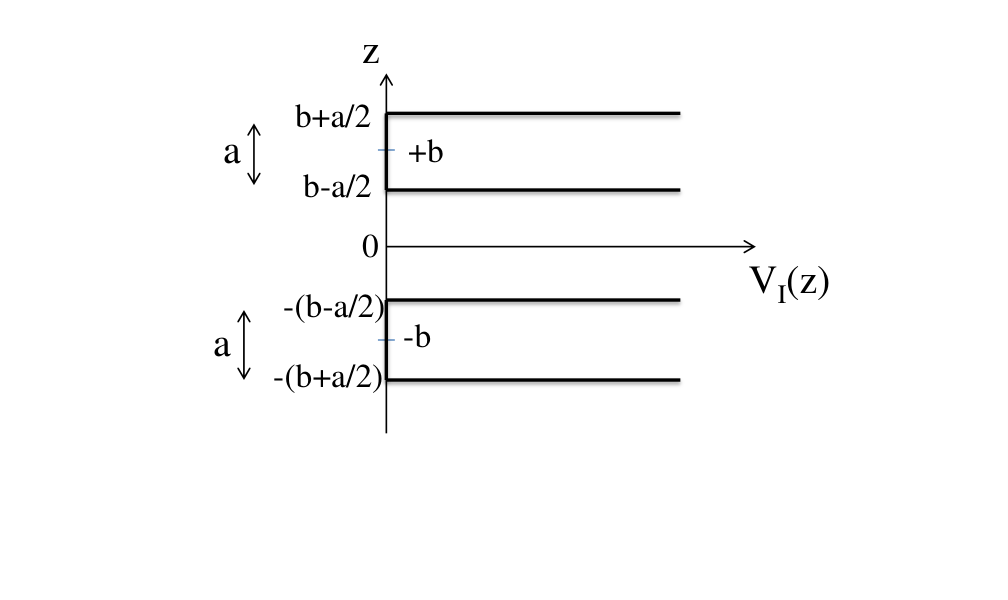
System electron has gained an average momentum $\gamma B_{i}\frac{\hbar}{2}\tau$ and hence its average kinetic energy is $\frac{p_{z}^{2}}{2M}=\frac{1}{2M}(\gamma B_{i}\frac{\hbar}{2}\tau)^{2}$, where all the parameters are known. We can choose the values of free parameters $a,b,B_{i}$ and $\tau$ (as explained below eq. 18), such that the system electron enters one of the eigenstates of the system Hamiltonian:

$$H_{0S}=\dfrac{p_{z}^{2}}{2M}+V_{I}(z)$$

(16)

where, $V_{I}(z)$ is as given in eq. 15. State of the system electron after trapping it in double well potential is given by,

	$\displaystyle|{\Phi_{0sn}(z)}\rangle=\cos\frac{\theta_{m}}{2}|{0}\rangle\left[\theta(z-(b-\frac{a}{2}))-\theta(z-(b+\frac{a}{2}))\right]\sqrt{\frac{2}{a}}\sin\big(k_{0sn}(b+\frac{a}{2}-z)\big)$
	$\displaystyle+\sin\frac{\theta_{m}}{2}e^{i\phi_{m}}|{1}\rangle\left[\theta(z+(b+\frac{a}{2}))-\theta(z+(b-\frac{a}{2}))\right]\sqrt{\frac{2}{a}}\sin\big(k_{0sn}(b+\frac{a}{2}+z)\big)$		(17)

where, $k_{0sn}=\frac{n\pi}{a},~n=1,2,3,...$. Unit step function is defined as,

$\displaystyle\theta(z-z_{0})=\begin{cases}0,~\mathrm{for}~z<z_{0}\\ 1,~\mathrm{for}~z>z_{0}\\ \end{cases}$

(18)

which implies $\frac{d}{dz}\theta(z-z_{0})=\delta(z-z_{0})$, Dirac-Delta function. We note that, even though $H_{0S}$ commutes with parity operator, its eigenstate $|{\Phi_{0sn}(z)}\rangle$ is not symmetric due to entanglement with spin d.o.f. Similarly $|{\Phi_{0an}(z)}\rangle$ (19) is not antisymmetric. Eq. 17 describes the superposition state of system electron being in upper and lower potential wells, while entangled with its spin degree of freedom. When $\theta_{m}=0$ or $\pi$, there is no splitting of the wave packet and eq. 17 reduces to the correct form describing the unsplit wave packet inside the potential well.

Inside the double well potential (excluding the boundary points, as derivative of the wave function does not exist there) $H_{0S}=\dfrac{p_{z}^{2}}{2M}=-\frac{\hbar^{2}}{2M}\frac{d^{2}}{dz^{2}}$ and it is easy to check, using $\frac{d}{dz}\theta(z-z_{0})=\delta(z-z_{0})$, that the state $|{\Phi_{osn}(z)}\rangle$ given in eq.17 is an eigenket of $H_{0S}$ with eigenvalue $E_{n}=\frac{\hbar^{2}k_{0sn}^{2}}{2M}$.

We can make the system electron to enter the eigenstate $|{\Phi_{0sn}(z)}\rangle$ of $H_{0S}$, by choosing $E_{n}=\frac{p_{z}^{2}}{2M}=\frac{1}{2M}(\gamma B_{i}\frac{\hbar}{2}\tau)^{2}$ and following an argument similar to that carried out from eq. 32 to 35 with the limit $V_{0}\rightarrow\infty$ (here we also take the limit $\Delta p_{z}\rightarrow 0$. However, this is not necessary if we follow a different technique as explained in para next to next to eq. 35). Hence, in principle we can push the system electron into one of the eigenstates of $H_{0S}$.
Wavefunction in eq. 17 is Square Integrable unlike the plane waves $\exp(\frac{i}{\hbar}p_{z}z)$ and hence represents the actual physical state of system electron. Hence there is no need to construct a wave packet using the eigenkets $\{|{\Phi_{0sn}(z)}\rangle\}$, to represent the physical state of system electron inside the potential well, unlike the situation when the electron was free. This justifies our assumption that system electron enters the eigenstate given in eq. 17, inside the potential well. This can be further justified by the fact that, an electron in a bound state of hydrogen atom can exist in one of the eigenstates, even though it was in a superposition of infinite number of plane waves $\exp(\frac{i}{\hbar}\vec{p}.\vec{r})$ when it was unbounded.

Completeness of eigenstates of $H_{0S}$: Using eq.17, taking the inner product of $|{\Phi_{0sk}(z)}\rangle$ with $|{\Phi_{0sn}(z)}\rangle$ which involves integration w.r.t $z$ from $-\infty$ to $+\infty$, we get $\langle{\Phi_{0sk}(z)}|{\Phi_{0sn}(z)}\rangle=\delta_{kn}$, where $\delta_{kn}$ is the kronecker delta function, and hence orthonormal. In eq. 17 if we introduce a relative phase ($e^{i\pi}$) between two terms (which is equivalent to changing $\theta_{m}$ to $-\theta_{m}$), we get a normalized solution which is linearly independent from $|{\Phi_{0sn}(z)}\rangle$. Then using Grahm-Schmidt orthogonalization, the solution becomes:

	$\displaystyle|{\Phi_{0an}(z)}\rangle=\sin\frac{\theta_{m}}{2}|{0}\rangle\left[\theta(z-(b-\frac{a}{2}))-\theta(z-(b+\frac{a}{2}))\right]\sqrt{\frac{2}{a}}\sin\big(k_{0an}(b+\frac{a}{2}-z)\big)$
	$\displaystyle-\cos\frac{\theta_{m}}{2}e^{i\phi_{m}}|{1}\rangle\left[\theta(z+(b+\frac{a}{2}))-\theta(z+(b-\frac{a}{2}))\right]\sqrt{\frac{2}{a}}\sin\big(k_{0an}(b+\frac{a}{2}+z)\big)$		(19)

where $k_{0an}=\frac{n\pi}{a},~n=1,2,3,...$. One can verify that $|{\Phi_{0an}(z)}\rangle$ is an eigenket of $H_{0S}$, with eigenvalue same as that corresponding to the state $|{\Phi_{0sn}(z)}\rangle$, and hence degenerate with it. One can also verify that $\langle{\Phi_{0ak}(z)}|{\Phi_{0an}(z)}\rangle=\delta_{kn}$ and $\langle{\Phi_{0sk}(z)}|{\Phi_{0an}(z)}\rangle=0$ for all $k,n$ and hence mutually orthogonal. Using the relation:

	$\displaystyle\sum\limits_{n=1}^{\infty}\sqrt{\frac{2}{a}}\sin\big(\frac{n\pi}{a}z\big)\sqrt{\frac{2}{a}}\sin\big(\frac{n\pi}{a}z^{\prime}\big)\left[\theta(z)-\theta(z-a)\right]\left[\theta(z^{\prime})-\theta(z^{\prime}-a)\right]=\delta(z^{\prime}-z)\left[\theta(z)-\theta(z-a)\right]\left[\theta(z^{\prime})-\theta(z^{\prime}-a)\right]$
			(20)

where, $\delta(z^{\prime}-z)$ is the Dirac delta function, one can verify that:

	$\displaystyle\sum\limits_{n=1}^{\infty}\bigg(|{\Phi_{0sn}(z)}\rangle\langle{\Phi_{0sn}(z^{\prime})}|+|{\Phi_{0an}(z)}\rangle\langle{\Phi_{0an}(z^{\prime})}|\bigg)=|{0}\rangle\langle{0}|\delta(z^{\prime}-z)\left[\theta(z-(b-\frac{a}{2}))-\theta(z-(b+\frac{a}{2}))\right]$
	$\displaystyle\left[\theta(z^{\prime}-(b-\frac{a}{2}))-\theta(z^{\prime}-(b+\frac{a}{2}))\right]+|{1}\rangle\langle{1}|\delta(z^{\prime}-z)\left[\theta(z+(b+\frac{a}{2}))-\theta(z+(b-\frac{a}{2}))\right]$
	$\displaystyle\left[\theta(z^{\prime}+(b+\frac{a}{2}))-\theta(z^{\prime}+(b-\frac{a}{2}))\right]~~~~~~\Rightarrow\int\limits_{-\infty}^{\infty}dz^{\prime}\sum\limits_{n=1}^{\infty}\bigg(|{\Phi_{0sn}(z)}\rangle\langle{\Phi_{0sn}(z^{\prime})}|+|{\Phi_{0an}(z)}\rangle\langle{\Phi_{0an}(z^{\prime})}|\bigg)=\mathbbm{1}$		(21)

where, $\mathbbm{1}$ is $2\times 2$ identity matrix, there by satisfying the completeness relation.

To measure a given system protectively, system should be in a non-degenerate eigenstate of system Hamiltonian. But the state $|{\Phi_{0sn}(z)}\rangle$, which we want to measure protectively, is a degenerate eigenstate of $H_{0S}$, as discussed in previous paragraph. If we perturb the system by applying a small negative potential in the region $-(b-\frac{a}{2})\leq z\leq(b-\frac{a}{2})$, degeneracy will be lifted due to tunneling. Adding a small negative potential to a very large but finite potential(which is infinite for all practical purposes), lowers the net potential slightly, there by allowing tunneling. Instead of solving perturbatively (for perturbative treatment see [10]), we are going to treat the potential in the region $-(b-\frac{a}{2})\leq z\leq(b-\frac{a}{2})$ to be $V_{0}(>0)$, which is finite and constant, and solve exactly. If necessary, later we can take $V_{0}$ to be very large but finite, to satisfy the condition of small perturbation to $V_{I}(z)$ (15). Following treatment is similar to that on pp460-62 of [10]. We are going to find the eigenstates $|{\phi_{sn}(z)}\rangle$, $|{\phi_{an}(z)}\rangle$ of new system Hamiltonian:

$$H_{S}=\dfrac{p_{z}^{2}}{2M}+V_{F}(z)$$

(22)

with eigenvalues $E_{sn}$ and $E_{an}$ respectively, which are less than $V_{0}$. $V_{F}(z)$ is same as $V_{I}(z)$ given in eq. 15 but $V_{F}(z)=V_{0}$ in the region $-(b-\frac{a}{2})\leq z\leq(b-\frac{a}{2})$ instead of $\infty$.

As the system electron is in superposition of being in both wells, it can tunnel from both wells into the region $-(b-a/2)<z<(b-a/2)$. As the split wave packets tunnel into the region $-(b-a/2)<z<(b-a/2)$, they get united and hence disentangles from spin d.o.f. This is justified by the fact that, if we reverse the direction of inhomogeneous magnetic field (see above eq. 53), the split wave packets start moving towards the origin, get united and hence disentangles from spin d.o.f. With this requirement, $|{\Phi_{0sn}(z)}\rangle$ (17) suggests the following form for one of the eigenstates of $H_{S}$ with energy $E_{s}<V_{0}$:

	$\displaystyle|{\phi_{s}(z)}\rangle=\cos\frac{\theta_{m}}{2}|{0}\rangle\left[\theta(z-(b-\frac{a}{2}))-\theta(z-(b+\frac{a}{2}))\right]A~\sin\big(k_{s}(b+\frac{a}{2}-z)\big)$
	$\displaystyle+\sin\frac{\theta_{m}}{2}e^{i\phi_{m}}|{1}\rangle\left[\theta(z+(b+\frac{a}{2}))-\theta(z+(b-\frac{a}{2}))\right]A^{\prime}~\sin\big(k_{s}(b+\frac{a}{2}+z)\big)$
	$\displaystyle+(\cos\frac{\theta_{m}}{2}|{0}\rangle+\sin\frac{\theta_{m}}{2}e^{i\phi_{m}}|{1}\rangle)\left[\theta(z+(b-\frac{a}{2}))-\theta(z-(b-\frac{a}{2}))\right](B~e^{q_{s}(z-b)}+B^{\prime}~e^{-q_{s}(z-(-b))})$		(23)

where, $q_{s}=\sqrt{\frac{2M}{\hbar^{2}}(V_{0}-E_{s})}=\sqrt{\alpha^{2}-k_{s}^{2}}~>0$. We have related energy $E_{s}$ of the state with its wave number $k_{s}$ by the relation:

$$E_{s}=\frac{\hbar^{2}k_{s}^{2}}{2M}$$

(24)

Exponentially decaying wave $e^{q_{s}(z-b)}$ corresponds to tunnelling from upper potential well (i.e., potential well on positive $z$-axis) into the region $-(b-\frac{a}{2})\leq z\leq(b-\frac{a}{2})$ and $e^{-q_{s}(z-(-b))}$ corresponds to that from lower well. Further, $|{\Phi_{0sn}(z)}\rangle$ (17) suggests to take $A=A^{\prime}=A_{s}$ and $B=B^{\prime}=B^{\prime}_{s}$ in eq. 23. Evanescent wave reduces to the form: $B~e^{q_{s}(z-b)}+B^{\prime}~e^{-q_{s}(z-(-b))}=B_{s}~\cosh(q_{s}z)$, where $B_{s}=2B^{\prime}_{s}e^{-q_{s}b}$. It is evident that in the limit $V_{0}$ (hence $q_{s}$) going to infinity, both evanescent waves vanish and we recover the state in eq. 17 as required. Demanding that the spatial wave function and its first derivative must be continuous at $z=b-\frac{a}{2}$, we obtain the following constraint equation:

$\displaystyle\tan(k_{s}a)=-\dfrac{k_{s}}{\sqrt{\alpha^{2}-k^{2}_{s}}}\coth\big(\sqrt{\alpha^{2}-k^{2}_{s}}(b-\frac{a}{2})\big)~~~~~~~~~$

(25)

This follows from the fact that $A_{s}$ and $B_{s}$ cannot vanish simultaneously, else we get trivial solution $|{\phi_{s}(z)}\rangle=0$ everywhere. Also in obtaining eq. 25 we dropped unit step function which is justifiable as it is used just for the sake of convenience. Similar joining conditions at $z=-(b-\frac{a}{2})$, also gives same constraint eq. 25.
Now, $|{\Phi_{0an}(z)}\rangle$ (19) suggests the following form for another eigenstate of $H_{S}$ (which is linearly independent from $|{\phi_{s}(z)}\rangle$ 23) with energy $E_{a}<V_{0}$:

	$\displaystyle|{\phi_{a}(z)}\rangle=\sin\frac{\theta_{m}}{2}|{0}\rangle\left[\theta(z-(b-\frac{a}{2}))-\theta(z-(b+\frac{a}{2}))\right]A~\sin\big(k_{a}(b+\frac{a}{2}-z)\big)$
	$\displaystyle+\cos\frac{\theta_{m}}{2}e^{i\phi_{m}}|{1}\rangle\left[\theta(z+(b+\frac{a}{2}))-\theta(z+(b-\frac{a}{2}))\right]A^{\prime}~\sin\big(k_{a}(b+\frac{a}{2}+z)\big)$
	$\displaystyle+(\sin\frac{\theta_{m}}{2}|{0}\rangle+\cos\frac{\theta_{m}}{2}e^{i\phi_{m}}|{1}\rangle)\left[\theta(z+(b-\frac{a}{2}))-\theta(z-(b-\frac{a}{2}))\right](B~e^{q_{a}(z-b)}+B^{\prime}~e^{-q_{a}(z-(-b))})$		(26)

where, $q_{a}=\sqrt{\frac{2M}{\hbar^{2}}(V_{0}-E_{a})}=\sqrt{\alpha^{2}-k_{a}^{2}}~>0$, $E_{a}=\hbar^{2}k_{a}^{2}/(2M)$. $|{\Phi_{0an}(z)}\rangle$ (19) suggests to take $A^{\prime}=-A=-A_{a}$ and $B^{\prime}=-B=-B^{\prime}_{a}$. With this, evanescent wave takes the form: $B~e^{q_{a}(z-b)}+B^{\prime}~e^{-q_{a}(z-(-b))}=B_{a}~\sinh(q_{a}z)$, where, $B_{a}=2B^{\prime}_{a}e^{-q_{a}b}$. In the limit $V_{0}\rightarrow\infty$, $|{\phi_{a}(z)}\rangle$ (26) reduces to $|{\Phi_{0an}(z)}\rangle$ (19) as required. Applying joining conditions at $z=b-\frac{a}{2}$ in a manner similar to previous case, we obtain the following constraint equation:

$\displaystyle\tan(k_{a}a)=-\dfrac{k_{a}}{\sqrt{\alpha^{2}-k^{2}_{a}}}\tanh\big(\sqrt{\alpha^{2}-k^{2}_{a}}(b-\frac{a}{2})\big)~~~~~~~~~$

(27)

Joining conditions at $z=-(b-\frac{a}{2})$ also leads to same constraint eq. 27. Equtions 25 and 27 can be solved graphically for $k_{s}$ and $k_{a}$ respectively, to obtain $k_{sn}$ and $k_{an}$ as $n^{th}$ roots, there by quantizing the energy levels. As constraint eq.s 25 and 27 are not identical in form, $k_{sn}$ will not be equal to $k_{an}$. Then, using relation 24 and $E_{a}=\hbar^{2}k_{a}^{2}/(2M)$, we obtain $E_{sn}\neq E_{an}$, there by lifting degeneracy. In the limit $V_{0}\rightarrow\infty$, we obtain from eq.s 25 and 27: $k_{s,a}\rightarrow\frac{n\pi}{a}$ as required. As $q_{sn,an}>0$ we have $E_{sn,an}<V_{0}$. Eigenstates of $H_{S}$, given by eqs. 23 and 26, take the following form after quantization:

	$\displaystyle|{\phi_{sn}(z)}\rangle=|{\phi_{0sn}(z)}\rangle+|{\hat{m}}\rangle B_{sn}~\cosh(q_{sn}z)~~~~~~~~~$
	$\displaystyle\left[\theta(z+(b-\frac{a}{2}))-\theta(z-(b-\frac{a}{2}))\right],~~~~~~$
	$\displaystyle|{\phi_{an}(z)}\rangle=|{\phi_{0an}(z)}\rangle+(\sin\frac{\theta_{m}}{2}|{0}\rangle+\cos\frac{\theta_{m}}{2}e^{i\phi_{m}}|{1}\rangle)~~~~$
	$\displaystyle B_{an}~\sinh(q_{an}z)\left[\theta(z+(b-\frac{a}{2}))-\theta(z-(b-\frac{a}{2}))\right]~~~~~~~$		(28)

where, $|{\hat{m}}\rangle$ is given by eq. 12, and:

	$\displaystyle|{\phi_{0sn}(z)}\rangle=\cos\frac{\theta_{m}}{2}|{0}\rangle\left[\theta(z-(b-\frac{a}{2}))-\theta(z-(b+\frac{a}{2}))\right]A_{sn}~\sin\big(k_{sn}(b+\frac{a}{2}-z)\big)$
	$\displaystyle+\sin\frac{\theta_{m}}{2}e^{i\phi_{m}}|{1}\rangle\left[\theta(z+(b+\frac{a}{2}))-\theta(z+(b-\frac{a}{2}))\right]A_{sn}~\sin\big(k_{sn}(b+\frac{a}{2}+z)\big),$
	$\displaystyle|{\phi_{0an}(z)}\rangle=\sin\frac{\theta_{m}}{2}|{0}\rangle\left[\theta(z-(b-\frac{a}{2}))-\theta(z-(b+\frac{a}{2}))\right]A_{an}~\sin\big(k_{an}(b+\frac{a}{2}-z)\big)$
	$\displaystyle-\cos\frac{\theta_{m}}{2}e^{i\phi_{m}}|{1}\rangle\left[\theta(z+(b+\frac{a}{2}))-\theta(z+(b-\frac{a}{2}))\right]A_{an}~\sin\big(k_{an}(b+\frac{a}{2}+z)\big)$		(29)

In the limit $V_{0}\rightarrow\infty$, we obtain $|{\phi_{sn}(z)}\rangle\rightarrow|{\Phi_{0sn}(z)}\rangle$ and $|{\phi_{an}(z)}\rangle\rightarrow|{\Phi_{0an}(z)}\rangle$ as required. One can verify that $\langle{\phi_{ak}(z)}|{\phi_{sn}(z)}\rangle=0$, for all $k,n$. However, $\langle{\phi_{sk}(z)}|{\phi_{sn}(z)}\rangle\neq 0$ and $\langle{\phi_{ak}(z)}|{\phi_{an}(z)}\rangle\neq 0$, for $k\neq n$. We can make them zero via Grahm-Schmidt orthogonalization. Arbitrary constants $A_{sn},A_{an},B_{sn}$ and $B_{an}$ can be fixed by the requirement that each of the states $\left\{|{\phi_{sn}(z)}\rangle,|{\phi_{ak}(z)}\rangle\right\}$, for all $s,k$, be normalised and satisfy completeness relation along with the states $\left\{|{\phi^{\prime}_{l}(z)}\rangle\right\}$, where $|{\phi^{\prime}_{l}(z)}\rangle=|{\hat{m}}\rangle\sqrt{\frac{2}{2b+a}}\cos(\frac{l\pi}{2b+a}z)$ is an eigenstate of $H_{S}$ with eigenvalue $E^{\prime}_{l}>V_{0}$. Also $\langle{\phi^{\prime}_{l}(z)}|{\phi_{sn,an}(z)}\rangle\neq 0$. Taking the state of our main interest, $|{\phi_{s1}(z)}\rangle$, as reference, we can orthogonalize the complete set $\left\{|{\phi_{sk}(z)}\rangle,|{\phi_{ak}(z)}\rangle,|{\phi^{\prime}_{l}(z)}\rangle\right\}$ via Grahm-Schmidt orthogonalization. The set $\left\{|{\phi_{sk}(z)}\rangle,|{\phi_{ak}(z)}\rangle,|{\phi^{\prime}_{l}(z)}\rangle\right\}$, after orthonormalization, should satisfy the completeness relation analogous to that in eq. 21, i.e.,

	$\displaystyle\int\limits_{-\infty}^{\infty}dz^{\prime}\bigg[\sum\limits_{k=1}^{M}\bigg(|{\phi_{sk}(z)}\rangle\langle{\phi_{sk}(z^{\prime})}|+|{\phi_{ak}(z)}\rangle\langle{\phi_{ak}(z^{\prime})}|\bigg)+~~~~~$
	$\displaystyle\sum\limits_{l=2M+1}^{\infty}|{\phi^{\prime}_{l}(z)}\rangle\langle{\phi^{\prime}_{l}(z^{\prime})}|\bigg]=\int\limits_{-\infty}^{\infty}dz^{\prime}\sum\limits_{i=1}^{\infty}|{\phi^{\prime\prime}_{i}(z)}\rangle\langle{\phi^{\prime\prime}_{i}(z^{\prime})}|=\mathbbm{1}~~~~~~$		(30)

	$\displaystyle\mathrm{where},~|{\phi_{sk}(z)}\rangle=|{\phi^{\prime\prime}_{2k-1}(z)}\rangle,~|{\phi_{ak}(z)}\rangle=|{\phi^{\prime\prime}_{2k}(z)}\rangle,$
	$\displaystyle|{\phi^{\prime}_{l}(z)}\rangle=|{\phi^{\prime\prime}_{l}(z)}\rangle~~~~~~~~~~~~~~~$		(31)

We can justify this by the fact that, in the limit $V_{0}\rightarrow\infty$ we recover the completeness relation in eq. 21, which corresponds to $V_{I}(z)$ (15). By perturbing $V_{I}$ with a small negative potential, we obtain the case of finite potential, $V_{F}(z)$ (22). As perturbation doesnot destroy the completeness property of the set of states being perturbed, completeness relation in eq. 30 is justified.

References

- [1] J. D. Barrow et al., Science and Ultimate Reality (Cambridge University Press, 2004).
- [2] J. Audretsch, Entangled Systems: New Directions in Quantum Physics (Wiley, 2007).
- [3]
One can easily verify that this satisfies equations in 2, and it is possible to decompose it as in eq. 3.(71) - [4]
It is not possible to know the operator apriori, as it is a function of unknown parameters and . In the protocol that we are going to describe, we will come to know and , only at the end. The whole chain of complex processes involved in the protocol, may not be representable by a simple operator like . Here we are just trying to motivate mathematically and may not have any relevance to physical reality at all!(72) - [5] H. Fan et al., Physics Reports 544, 241 (2014).
- [6]
Let be a macroscopic measuring device with very large
number of d.o.f (as it amplifies the information) which measures
(-component of total spin angular momentum operator). Then we have:
and . Now consider:
Hence measurement operator , is a nonlinear operator, as it breaks the superposition. In the protocol that we are going to describe, probe electron starts with (footnote below eq. 52) and it will not get entangled with system electron, but still gains momentum proportional to . As explained in footnote below eq. 52, in principle it is possible to measure this momentum (and hence ) with arbitrary precision. This can be represented as: (this is similar to ), where, is a macroscopic measuring device similar to , and is the state of probe electron. This shows there is no collapse (as no entanglement any where) upon measuring probe electron and hence we are able to get with probability one. This does not mean that we have obtained the value of with a linear operation (as no collapse has occured), because is intrinsically a nonlinear operator. Its nonlinearity has not been explicitly displayed, because our protocol was such that it avoided entanglement all the way. It is similar to the following situation: Let . This does not mean that is a linear function. We have chosen the values in such a way that the function appears to behave like a linear function. Now, has to be solved for using an equation similar to 52. This process of solving (which is very much part of cloning) is a macroscopic phenomenon (measurement) which involves directly or indirectly collapse of wave function (eg., as we write down the equation on a piece of paper, we are collapsing the state of atoms of ink, which otherwise can exist anywhere in the universe with nonzero probability, however small), there by nonlinear processes explicitly come into picture. There are still many such processes which directly or indirectly involve nonlinear processes (which are also very much part of cloning) like, solving constraint equations 54, 59, and, clubbibg the information and preparing another qubit in the state . We also note that, according to Everett’s many-worlds interpretation and Bohm’s causal interpretation of quantum measurement [7], there is no breaking of superposition at the level of consciousness and matter respectively, and hence no nonlinearity. However, we believe that, as we cannot observe superposed states, some where nonlinearity has to come in, either at the level of matter or consciousness.(73) (74) - [7] D. Home, Conceptual Foundations of Quantum Physics chapter 2 (Springer Science and Business media, 1997).
- [8] Y. Aharonov and L. Vaidman, Physics Letters A 178, 38 (1993).
- [9] Y. Aharonov, J. Anandan, and L. Vaidman, Phys. Rev. A 47, 4616 (1993).
- [10] C. Cohen Tannoudji et al., Quantum Mechanics vol. one and two (John Wiley and Sons, 2005).
- [11] In an actual Stern Gerlach apparatus both and . The field that satisfies these conditions is: ([30], p388 of [10]), where, . For , and hence spin precesses about -axis with frequency . As a result, -component of spin, , oscillates in time and hence its average over an interval of time large compared to period of oscillation () but small compared to , vanishes. Only survives. Hence wave packet splits only along -axis. Due to the precence of static field , unknown spin precesses about -axis, which can be easily taken into account. Hence we are not going to consider the effect of static field.
- [12] From the previous footnote it is evident that actual interaction energy, . Eigenvalues os are . As the reference point can always be shifted, we consider only the difference in energy levels which is: as . Hence we can write: . As can be arbitrarily large, can also be made arbitrarily large for any . Hence, holds for any , .
- [13] L. Hardy, Physics Letters A 167, 11 (1992).
- [14] This can also be justified as follows: Consider a Box normalized plane wave: with periodic boundary condtion. It is the spatial wave function of system electron. It is an eigenstate of with discrete energy , where, , . is the length of box, which is large but finite. Spacing between the energy levels can be made as small as we want by increasing [24]. Now switch on the inhomogeneous magnetic field for an interval of time , such that . Change the Hamiltonian of system electron from to with , in an interval of time . Then, by adiabatic theorem (see below eq. 40), system electron will end up in the eigenstate of : corresponding to .
- [15] N. D. Hari Dass and T. Qureshi, Phys. Rev. A 59, 2590 (1999).
- [16] To settle down to ground state, system electron has to emit photon(s). But system electron is already entangled with it’s spin d.o.f. Hence emission of photon may cause mutual entanglement between spin and spatial d.o.f of system electron, and photon. Then it may be necessary to measure protectively the combined three systems, which we are not considering here.
- [17] For eg., imagine a three dimensional (3D) double box potential, where, potential inside the box is zero, while infinite on the six walls of box. Box is opaque to matter wave (as trapped electron cannot escape), while transparent to electromagnetic field. Now, to break the degeneracy, connect the two boxes with a long tube, such that it does not obstruct the motion of probe electron. Inside the tube, potential is finite (), whereas infinite on its walls. This is analogous to the potential (eq. 22). Our protocol can be generalized to 3D double box potential case.
- [18] As a first step, to get an approximate solution, we are assuming that is relatively small, so that becomes time independent. In a more accurate solution we can treat as time dependent perturbation or handle it as a quantum electrodynamical problem, and we can handle arbitrarily large .
- [19] Initial state of probe electron (eq. 38) was a Gaussian minimum (i.e., ) wave packet centered at . Because , at any time : (see below eq. 44). We did calculations from eq. 45-52 assuming the spread to be small. However, in principle can be arbitrarily large, as the separation between potential wells can also be made arbitrarily large (below eq. 35) and one can handle it as QED problem or calculate the integral (44) to all orders in (spreading). Hence, in principle we can start with a squeezed minimum wave packet: with , and . After the interaction with system electron, to measure the momentum gained by probe electron, shine it with a photon of wavelength . By measuring the change in frequency, due to Doppler effect, of scattered photon we can calculate the velocity of probe electron. The change in momentum of probe electron (, which is also the error in momentum measurement) due to collision with photon, is inversely proportional to (Compton effect) [31]. In principle it is possible to take: . As a result, error: and the measured value of momentum of probe electron tends to . Of course, error in position measurement: (as ), in which any way we are not interested. Also, even in the limit , it is possible to make (36) goto zero as follows: Let the wave packet of probe electron be centered at with standard deviation . Then, maximum possible strength of is proportional to . As the separation between two potential wells can be made arbitrarily large, we can take . Now, in the limit (i.e., ), . We also note that, the requirement (hence, ) (below 35) demands width ‘’ to be of the order of . Hence, . In the limit and , also tends to infinity. This can be satisfied as can be arbitrarily large.
- [20] Let be the strength of (relation 36). In the nondegenerate perturbation theory, first order correction to goes as (p1101 of [10]). In the limit (i.e., ) evanescent wave goes to zero. As explained below relation 36, depends on separation between two wells, which can be made arbitrarily large, and hence arbitrarily small. We can choose the separation between two wells such that is numerically proportional to . Now, in the limit , both first order correction to and evanescent wave goes to zero. Similarly we can prove all higher order corrections to (p154 of [24]) also goes to zero. Also, criterion to treat as a small perturbation to is (p1096 [10]): . This is also satisfied by choosing numerically proportional to and taking the limit . Also, in the footnote below eq. 52, we took numerical value of (upper limit of ). Requirement that should goto zero, gave: . Equating this with above numerical value of , we obtain: . This puts a constraint on the rate at which should goto infinity or should goto zero i.e., the rates should be such that the product remains finite (). This can always be satisfied, for eg., taking numerical value of . Similarly, adiabaticity condition: (below eq. 40), can also be satisfied even in the limit , by choosing , which can also be arbitrarily large, numerically proportional to . Hence, evanescent wave is not a problem while recombining.
- [21] Even if we start with probe electron being a Gaussian minimum (i.e., ) wave packet, with , and (see footnote below eq. 52), as it interacts with system electron, it gains momentum and hence is no more zero. However, if (which might be possible by suitably choosing the free parameters and in (34). However, we note that is constrained by the requirement , by the weak measurement criterion and by adiabaticity requirement. As and can be arbitrarily large, inspite of these constraints there might be a possibility of choosing them such that is also satisfied.), then we can neglect evolution under . In an exact calculation one can take into account also (eg., treating it as a QED problem or following a procedure described in [15]) but the conclusions remain unaffected, because, presence of cannot cause entanglement between system and probe electrons. may cause wave packet to spread, which can be taken into account.
- [22] An arbitrary function inside the single potential well can be expanded as:. Substituting for from eq.20 and rearranging, we get the required expansion. Note that needs to be changed to .
- [23] D. J. Griffiths, Introduction to Quantum Mechanics (Prentice Hall, 1995).
- [24] L. I. Schiff, Quantum Mechanics (McGraw-Hill Book Company, 1955).
- [25] However we note that, in principle it is possible to take into account, complete spreading of wave packet during the time interval . For eg., if we treat it as a QED problem , we get exact solution or do the integral (44) to all orders in . However, to get an approximate solution, we consider spreading of wave packet only to first order in .
- [26] .
- [27] It is not an issue, as increase in can be compensated by increasing width ‘a’ of potential well, which can be arbitrarily large in principle.
- [28] Y. Aharonov, J. Anandan, and L. Vaidman, Foundations of Physics 26, 117 (1996).
- [29] J. A. Jones et al., Nature 403, 869 (2000).
- [30] D. E. Platt, American Journal of Physics 60, 306 (1992).
- [31] W. Heisenberg in, Quantum Theory and Measurement edited by J A Wheeler and W H Zurek p66 (Princeton university press, 1983).