跳到论文正文
W Papers独立论文阅读器 arXiv:1503.04371 论文正文 计算阅读时间 · 0%
引用这篇论文根据当前论文元数据生成,正式投稿前建议核对。


License: arXiv.org perpetual non-exclusive license
arXiv:1503.04371v2 [cs.IT] 02 Feb 2016

Uniform Random Number Generation from Markov Chains: Non-Asymptotic and Asymptotic AnalysesThanks: This paper was presented in part at 2014 Information Theory and Applications Workshop [1].

Masahito Hayashi ††thanks: The first author is with the Graduate School of Mathematics, Nagoya University, Japan. He is also with the Centre for Quantum Technologies, National University of Singapore, Singapore. e-mail:masahito@math.nagoya-u.ac.jp    Shun Watanabe ††thanks: The second author is with the Department of Computer and Information Sciences, Tokyo University of Agriculture and Technology, Koganei, Tokyo, Japan. He was with the Department of Information Science and Intelligent Systems, University of Tokushima, Tokushima, Japan. e-mail:e-mail: shunwata@cc.tuat.ac.jp††thanks: Manuscript received ; revised
Abstract

In this paper, we derive non-asymptotic achievability and converse bounds on the random number generation with/without side-information. Our bounds are efficiently computable in the sense that the computational complexity does not depend on the block length. We also characterize the asymptotic behaviors of the large deviation regime and the moderate deviation regime by using our bounds, which implies that our bounds are asymptotically tight in those regimes. We also show the second order rates of those problems, and derive single letter forms of the variances characterizing the second order rates. Further, we address the relative entropy rate and the modified mutual information rate for these problems.

Index Terms: 
Markov Chain, Non-Asymptotic Analysis, Random Number Generation,

I Introduction

I-A Uniform random number generation (URNG)

Uniform random number generation is one of important tasks for information theory as well as secure communication. When a non-uniform random number is generated subject to independent and identical distribution and the source distribution is known to PXP_{X}, we can convert it to the uniform random number, whose optimal conversion rate is known to be the entropy H⁡(PX)H(P_{X}) [2]. Vembu and Verdú [3] extended this problem to the general information source. Applying their result to the Markovian source, we find that the optimal conversion rate is the entropy rate.

On the other hand, many researchers in information theory are attracted by non-asymptotic analysis recently [4, 5, 6]. Since all of realistic situations are non-asymptotic, it is strongly desired to evaluate the performance of a protocol in the non-asymptotic setting. In the case of uniform random number generation, we need to consider two issues:

A1)

How to quantitatively guarantee the security for finite block length nn. As the criterion, we employ the variational distance criterion because it is universal composable[7].

A2)

How to implement the extracting method efficiently.

Fortunately, the latter problem has been solved by employing universal2 hash functions, which can be constructed by combination of Toeplitz matrix and the identity matrix [8]. This construction has small amount of complexity and was implemented in a real demonstration [9, 10]. Recently, the paper [11] proposed a new class of hash functions, ε\varepsilon-almost dual universal hash functions, and the paper [10] proposed more efficient hash functions belonging to this new class. Hence, it is needed to solve the first problem.

So far, with a huge size nn, quantitative evaluation of the security has been done only for the i.i.d. source [8, 12]. However, the source is not necessarily i.i.d. in the real world, and it is necessary to develop a technique to evaluate the security for non i.i.d. source. As a first step of this direction of research, we consider the Markov source in this paper. In the following, we explain difficulties to extend the existing results for the i.i.d. source to the Markov source.

Although it is not stated explicitly in any literatures, we believe that there are two important criteria for non-asymptotic bounds:

B1)

Computational complexity, and

B2)

Asymptotic optimality.

Let us first consider the first criterion, i.e., the computational complexity. For example, Han [13] introduced lower and upper bounds for the variational distance criterion by using the inf-spectral entropy, which are called the inf-spectral entropy bounds. For i.i.d. sources, these bounds can be computed by numerical calculation packages. However, there is no known method to efficiently compute these bounds for Markov sources. Consequently, there is no bound that is efficiently computable for the Markov chain so far. The first purpose of this paper is to derive non-asymptotic bounds that are efficiently computable.

Next, let us consider the second criterion, i.e., asymptotic optimality. So far, three kinds of asymptotic regimes have been studied in the information theory:

B2-1)

The large deviation regime in which the error probability ε\varepsilon asymptotically behaves like e−n​re^{-nr} for some r>0r>0 [14],

B2-2)

The moderate deviation regime in which ε\varepsilon asymptotically behaves like e−n1−2​t​re^{-n^{1-2t}r} for some r>0r>0 and t∈(0,1/2)t\in(0,1/2) [15, 16, 17], and

B2-3)

The second order regime in which ε\varepsilon is a constant [18, 4, 5, 6, 15, 16, 19].

We shall claim that a good non-asymptotic bound should be asymptotically optimal in at least one of the above mentioned three regimes.

Further, when the generation rate is too large, the variational distance is close to 11. In this case, we cannot measure how far from the uniform random number the generated random number is. Hence, we employ the relative entropy rate (RER).

I-B Secure uniform random number generation (SURNG)

When the initial random number XX is partially leaked to the third party YY, to guarantee the security, we need to convert the random number to the uniform random number that has almost no correlation with the third party. When a non-uniform random number is generated subject to independent and identical distribution of the joint distribution is known to PX,YP_{X,Y}, we can convert it to the uniform random number, whose optimal conversion rate is known to be the conditional entropy H⁡(X|Y)H(X|Y) [20, 21].

Bennett et al. [22, 23] and Håstad et al. [24] proposed to use universal2 hash functions for this purpose, and derived two universal hashing lemma, which provides an upper bound for leaked information based on Rényi entropy of order 22. The paper [11] proposed to use ε\varepsilon-almost dual universal hash functions [11] that includes the hash functions by [10]. Hence, the problem A2) has been solved by employing universal2 hash functions.

Therefore, the remaining problem is the problem A1), i.e., to quantitatively guarantee the security for finite block length nn under these hash functions. For the security criterion, we employ the variational distance between the true distribution and the ideal distribution because it satisfies the universal composable property [7]. To achieve the rate H⁡(X|Y)H(X|Y) via two universal hashing lemma, Renner [25] attached the smoothing to min entropy11 1 Bennett et al. [23] also employed a similar idea without use of the terminology of smoothing, and derived the conversion rate H⁡(X|Y)H(X|Y)., which is a lower bound on the above conditional Rényi entropy of order 2222 2 In [25], Renner also showed a quantum extension of the two universal hashing lemma.. That is, he proposed to maximize the min-entropy among the sub-distributions whose variational distance to the true distribution is less than a given threshold. Using Renner’s method, the paper [12] derived a lower bound of the exponential decreasing rate. Tomamichel and Hayashi [26] derived an upper bound of the universal composable quantity of extracted key with a finite block-length nn by combining the Renner’s method and the method of information spectrum by Han. Further, Watanabe and Hayashi [27] compared two approaches: the combination of the Renner’s method and the method of information spectrum33 3 The approach to derive a bound in [27] is almost the same as that in [26], but it should be noted that the security criterion in [27] is based on the variational distance while that in [26] is based on the purified distance., and the exponential bounding approach of [12]. Further, the paper [28] showed that similar evaluations are possible even for ε\varepsilon-almost dual universal hash functions [11].

For convenience, let us call the bound derived by the former approach the inf-spectral entropy bound, and the bound derived by the latter approach the exponential bound. It turned out that the exponential bound is tighter than the inf-spectral entropy bound when the required security level ε\varepsilon is rather small. A bound that interpolate both approaches was also derived in [27], which we called the hybrid bound.

Similar to uniform random number generation, for i.i.d. sources, the inf-spectral entropy bound and the hybrid bound can be computed by numerical calculation packages. However, there is no known method to efficiently compute these bounds for Markov sources. The computational complexity of the exponential bound is O⁡(1)O(1) since the exponential bound is described by using the Gallager function, which is an additive quantity. However, this is not the case for Markov sources. Consequently, there is no bound that is efficiently computable for the Markov chain so far. Further, the first order results for Markov sources have not been revealed as long as the authors know, and they are clarified in this paper.

Further, when the generation key rate is too large, the variational distance is close to 11. In this case, we cannot measure how far from the secure uniform random number the generated random number is. Hence, we employ the relative entropy between the generated random number and the ideal random number, which was introduced by Csiszár-Narayan [29] and is called the modified mutual information rate. Indeed, when we surpass axiomatic conditions, the leaked information measure must be this quantity [28].

I-C Main Contribution for Non-Asymptotic Analysis

Although there are several studies for finite-length analysis for URNG and SURNG, they did not discuss the Markovian chain. Indeed, while they derived several single-shot bounds, these bounds cannot be directly applied to the Markovian chain, because the bounds obtained by such applications are not computable at least in the the Markovian chain. Hence, we need to derive new finite-length bounds for the Markovian chain by modifying existing single-shot bounds. For this purpose, we adopt the structure similar to the paper [30], which addresses the source coding with Markov chain because this paper employs the common structure between the uniform random number generation and the source coding. Hence, the obtained results are also quite similar to those of the paper [30]. To derive non-asymptotic achievability bounds on the problems, we basically use the exponential type bounds for the single shot setting. When there is no information leakage, those exponential type bounds are described by the Rényi entropy. Thus, we need to evaluate Rényi entropy for the Markov chain. For this purpose, we introduce Rényi entropy for transition matrices, which is defined irrespective of initial distributions (cf. (27)). Then, we evaluate the Rényi entropy for the Markov chain in terms of the Rényi entropy for the transition matrix. From this evaluation, we can also find that the Rényi entropy rate for the Markov chain coincides with the Rényi entropy for the transition matrix. Note that the former is defined as the limit and the latter is single letter characterized.

When a part of information is leaked to the third party, to generate secure uniform random number, we consider two assumptions on transition matrices (see Assumption 1 and Assumption 2 of Section II). Although a computable form of the conditional entropy rate is not known in general, Assumption 1, which is less restrictive than Assumption 2, enables us to derive a computable form of the conditional entropy rate.

In the problems with side-information, exponential type bounds are described by conditional Rényi entropies. There are several definitions of conditional Rényi entropies (see [31, 32] for extensive review), and we use the one defined in [8] and the one defined by Arimoto [33]. We shall call the former one the lower conditional Rényi entropy (cf. (3)) and the latter one the upper conditional Rényi entropy (cf. (8)). To derive non-asymptotic bounds, we need to evaluate these information measures for the Markov chain. For this purpose, under Assumption 1, we introduce the lower conditional Rényi entropy for transition matrices (cf. (27)). Then, we evaluate the lower conditional Rényi entropy for the Markov chain in terms of its transition matrix counterpart. This evaluation gives non-asymptotic bounds for secure uniform random number generation under Assumption 1. Under more restrictive assumption, i.e., Assumption 2, we also introduce the upper conditional Rényi entropy for a transition matrix (cf. (34)). Then, we evaluate the upper Rényi entropy for the Markov chain in terms of its transition matrix counterpart. This evaluation gives non-asymptotic bounds that are tighter than those obtained under Assumption 1.

We also derive converse bounds for every problem by using the change of measure argument developed by the authors in the accompanying paper on information geometry [34, 35]. When there is no information leakage, the converse bounds are described by the Rényi entropy for transition matrices. When a part of information is leaked to the third party, we further introduce two-parameter conditional Rényi entropy and its transition matrix counterpart (cf. (14) and (38)). This novel information measure includes the lower conditional Rényi entropy and the upper conditional Rényi entropy as special cases.

In the problem of SURNG, instead of the RER, we employ the modified mutual information rate (MMIR), which was introduced by Csiszár and Narayan [29] and whose axiomatic characterization was obtained in the paper [28]. When the uniformity is guaranteed, this quantity is given by the equivocation rate introduced by Wyner [36]. When there is no information leakage, our lower and upper bounds are given by using the Rényi entropy for the Markov chain in terms of its transition matrix counterpart. When there exists information leakage, our lower and upper bounds are given by using the lower conditional Rényi entropy for the Markov chain in terms of its transition matrix counterpart under Assumption 1.

Here, we would like to remark on terminologies. There are a few ways to express exponential type bounds. In statistics or the large deviation theory, we usually use the cumulant generating function (CGF) to describe exponents. In information theory, we use the Gallager function or the Rényi entropies. Although these three terminologies are essentially the same and are related by change of variables, the CGF and the Gallager function are convenient for some calculations since they have good properties such as convexity. However, they are merely mathematical functions. On the other hand, the Rényi entropies are information measures including Shannon’s information measures as special cases. Thus, the Rényi entropies are intuitively familiar in the field of information theory. The Rényi entropies also have an advantage that two types of bounds (eg. (219) and (222)) can be expressed in a unified manner. For these reasons, we state our main results in terms of the Rényi entropies while we use the CGF and the Gallager function in the proofs. For readers’ convenience, the relation between the Rényi entropies and corresponding CGFs are summarized in Appendix A.

Overall, we summarize the contributions for non-asymptotic analysis in comparison to existing results as follows.

(1)

Finite-length bound: For URNG and SURNG, we derive finite-length bounds satisfying the conditions B1) and B2) for Markovian chain. Theorems in Subsections III-C and IV-C are classified to this type of results. All existing finite-length bounds with computable form are obtained with i.i.d. setting. Indeed, several single-shot bounds were obtained in a more general form. However, their computabilities have not been discussed in the Markovian case. At least, many of them, (e.g, Lemmas 16, 17, 18, 22, 23, 25, and 28) are not given in a computable form in the Markovian case.

(2)

Single-shot bound: In this paper, we employ several existing single-shot bounds. However, many of them cannot be given in a useful form. These bounds cannot be easily calculated at least in the Markovian case. To apply them to the Markovian case, we loosen these bounds. Lemmas 21, 24, 29 and 32 fall in this case. Since these bounds have a much simpler form than existing bounds, they might be applied to other cases. This discussion for the simplification is quite different from the case of source coding [30]. That is, this part has the most serious technical hardness compared to the paper [30] because the discussion in this paper is specialized to random number generation.

TABLE I: Summary of Asymptotic Results and Non-Asymptotic Bounds to Derive Asymptotic Results
Problem First Order Large Deviation Moderate Deviation Second Order RER/MMIR
URNG Solved Solved∗\mbox{Solved}^{*} (U2), O⁡(1)O(1) Solved, O⁡(1)O(1) Solved, Tail Solved, O⁡(1)O(1)
SURNG Solved (Ass. 1) Solved∗\mbox{Solved}^{*} (Ass. 2, U2), Solved (Ass. 1), Solved (Ass. 1), Solved (Ass. 1),
O⁡(1)O(1) O⁡(1)O(1) Tail O⁡(1)O(1)

URNG is the uniform random number generation without information leakage. SURNG is the secure uniform random number generation when a part of information is leaked to the third party.

I-D Main Contribution for Asymptotic Analysis

Among authors’ knowledge, there is no existing study for the asymptotic analysis with the Markovian chain with respect to URNG and SURNG except for the following. When the general sequence of single information sources, the asymptotic rate of URNG is characterized by Vembu and Verdú [3] and Han [13]. Since the asymptotic entropy rate of Markovian chain is known, we can calculate the asymptotic rate of URNG for the Markovian chain. However, further study with respect to URNG and SURNG has not been discussed for the Markovian chain nor the general sequence of information sources.

We can easily see that these non-asymptotic bounds yields the asymptotic optimal random number generation rate while the case with information leakage requires Assumption 1. For asymptotic analyses of the large deviation and the moderate deviation regimes, we derive the characterizations44 4 For the large deviation regime, we only derive the characterizations up to the critical rates. by using our non-asymptotic achievability and converse bounds, which implies that our non-asymptotic bounds are tight in the large deviation regime and the moderate deviation regime.

We also derive the second order rate. It is also clarified that the reciprocal coefficient of the moderate deviation regime and the variance of the second order regime coincide. Furthermore, a single letter form of the variance is clarified55 5 An alternative way to derive a single letter characterization of the variance for the Markov chain was shown in [37, Lemma 20]. It should be also noted that a single letter characterization can be derived by using the fundamental matrix [38]. .

The asymptotic results and the non-asymptotic results are summarized in Table I. As a part of the non-asymptotic results, the table focuses on the computational complexities of the non-asymptotic bounds. ”Solved∗\mbox{Solved}^{*}” indicates that those problems are solved up to the critical rates. ”Ass. 1” and ”Ass. 2” indicate that those problems are solved under Assumption 1 or Assumption 2. ”U2” indicates that the converse results are obtained only for the worst case of the universal two hash family (see (105) and (182)). ”O⁡(1)O(1)” indicates that both the achievability part and the converse part of those asymptotic results are derived from our non-asymptotic achievability bounds and converse bounds whose computational complexities are O⁡(1)O(1). ”Tail” indicates that both the achievability part and the converse part of those asymptotic results are derived from the information-spectrum type achievability bounds and converse bounds whose computational complexities depend on the computational complexities of tail probabilities.

Exact computations of tail probabilities are difficult in general though it may be feasible for a simple case such as an i.i.d. case. One way to approximately compute tail probabilities is to use the Berry-Esséen theorem [39, Theorem 16.5.1] or its variant [40]. This direction of research is still continuing [41, 42], and an evaluation of the constant was done in [42] though it is not clear how much tight it is. If we can derive a tight Berry-Esséen type bound for the Markov chain, we can derive a non-asymptotic bound that is asymptotically tight in the second order regime. However, the approximation errors of Berry-Esséen type bounds converge only in the order of 1/n1/\sqrt{n}, and cannot be applied when ε\varepsilon is rather small. Even in the cases such that exact computations of tail probabilities are possible, the information-spectrum type bounds are looser than the exponential type bounds when ε\varepsilon is rather small, and we need to use appropriate bounds depending on the size of ε\varepsilon. In fact, this observation was explicitly clarified in [27] for the random number generation with side-information. Consequently, we believe that our exponential type non-asymptotic bounds are very useful.

Further, we derive the asymptotic leaked information rate. When there is no information leakage, we discuss the RER, which is asymptotically given by the entropy rate. When there exists information leakage, we discuss the MMIR, which is asymptotically given by the conditional entropy rate under Assumption 1.

Overall, we summarize the contributions for asymptotic analysis in comparison to existing results as follows.

(1)

New bounds for Markovian case: For URNG and SURNG, we derive the optimal asymptotic performances in Subsections III-D, III-E, III-F, 19, III-G, IV-D, IV-E, IV-F, and IV-G under the four regimes, the large deviation regimes, the moderate deviation regimes, the second order regimes, and the asymptotic relative entropy rate regime (the asymptotic modified mutual information rate regime) for Markovian chain (with suitable conditions for SURNG). Except for the information spectrum approach, all existing asymptotic analyses with these three regimes assume the i.i.d. source. Further, analyses with the information spectrum approach derived only the general formulas, which did not derive any computable asymptotic bounds for these three regimes for the Markovian chain.

(2)

New bound even for i.i.d. case: Among the above asymptotic results, Theorem 30 is novel even for the i.i.d. case. This theorem gives the converse bound for large deviation for SURNG.

I-E Two criteria

In this paper, to consider a practical issue, we employ two criteria. In the channel coding, such a practical issue is discussed as a coding theory in a form separate from the fundamental issue. However, in the random number generation case, we can discuss the performance of hash functions with a small construction complexity in the same way as the fundamental issue. Such a practical issue is also the target of this paper. Usually, when we discuss a fundamental aspect of the topic of information theory, we focus only on the minimum leaked information among all of hash function, which is denoted by Δ⁡(M)\Delta(M) in this paper, whose precise definition will be given in Subsections III-A and IV-A. However, when we take account into the complexity of construction of protocol, we need to restrict hash functions into hash functions with a small construction complexity. Hence, it is desired to minimize the leaked information among a class of hash functions with small calculation complexity for its construction. In this paper we focus on the family of two-universal hash functions, named by the two-universal hash family ℱ{\cal F} because this family contains a hash function with a small construction complexity. However, this paper focuses on the worst leaked information Δ¯​(M)\overline{\Delta}(M) among the two-universal hash family ℱ{\cal F}, which is more important from a practical view point than the best case due to the following two reasons.

(1)

Usually, the optimal hash function depends on the source distribution. However, it is not easy to perfectly identify the source distribution. In such a case, instead of the optimal hash function, we need to choose a hash function that universally works well. If we apply a two-universal hash function, its leaked information is always better than the worst leaked information Δ¯​(M)\overline{\Delta}(M). Hence, if the quantity Δ¯​(M)\overline{\Delta}(M) is sufficiently close to the optimal case Δ⁡(M){\Delta}(M), we can say that any two-universal hash function universally works well.

(2)

Although the two-universal hash family ℱ{\cal F} contains a hash function with a small calculation complexity for its construction, any two-universal hash function does not necessarily have a small calculation complexity. If the quantity Δ¯​(M)\overline{\Delta}(M) is sufficiently close to the optimal case Δ⁡(M){\Delta}(M), we can take the priority to minimize the construction complexity among the two-universal hash family ℱ{\cal F} over the optimization of the leaked information.

In this paper, we show that the worst leaked information Δ¯​(M)\overline{\Delta}(M) is close to the minimum leaked information Δ⁡(M){\Delta}(M) in the moderate deviation and the second order. These results guarantee that any two-universal hash function has a sufficiently good performance. That is, they allow us to employ any two-universal hash function to achieve these asymptotic optimal performances. These results amplify our choice of hash function to achieve the asymptotically optimality.

I-F Organization of Paper and Notations

As preparation, we explain information measures for single-shot setting in Subsection II-A. Then, we address conditional Rényi entropies for transition matrix in Subsection II-B, and discuss the relation between these information measures and Markov chain in Subsection II-C. These information measures and their properties will be used in the latter sections. These contents were obtained in the paper [30], and their proofs are available in the paper [30]. However, the paper [30] did not address the conditional min entropy, which corresponds to the order parameter ∞\infty. So, in Subsections II-D and II-E, we discuss the relation between the limit of the conditional Rényi entropy and the conditional min entropy, which are new results and are shown in Appendix.

Section III addresses the uniform random number generation without information leakage. The obtained upper and lower bounds are numerically calculated in a typical example in this section. Then, Section IV proceeds to addresses the secure uniform random number generation with partial information leakage. As we mentioned above, we state our main result in terms of the Rényi entropies, and we use the CGFs and the Gallager function in the proofs. In Appendix A, the relation between the Rényi entropies and corresponding CGFs are summarized. The relation between the Rényi entropies and the Gallager function are explained as necessary. Proofs of some technical results are also shown in the rest of appendices.

A random variable is denoted by upper case letter, and its realization is denoted by lower case letter. The notation 𝒫⁡(𝒳){\cal P}({\cal X}) is the set of all distribution on alphabet 𝒳{\cal X}. The notation 𝒫¯​(𝒳)\bar{{\cal P}}({\cal X}) is the set of all non-negative sub-normalized functions on 𝒳{\cal X}. |𝒳||{\cal X}| represent the cardinality of the set 𝒳{\cal X}. The cumulative distribution function of the standard Gaussian random variable is denoted by

Φ⁡(t)=∫−∞t12​π​exp⁡[−x22]​𝑑x.\displaystyle\Phi(t)=\int_{-\infty}^{t}\frac{1}{\sqrt{2\pi}}\exp\left[-\frac{x^{2}}{2}\right]dx. (1)

Throughout the paper, the base of the logarithm is ee.

II Information Measures

In this section, we introduce information measures that will be used in Section III and Section IV. All of lemmas and theorems in this section except for Lemmas 15 and 12 and Theorem 6 were shown in [30].

II-A Information Measures for Single-Shot Setting

II-A1 Conditional Rényi entropy relative to a general distribution

In this section, we introduce conditional Rényi entropies for the single-shot setting. For more detailed review of conditional Rényi entropies, see [32]. For a correlated random variable (X,Y)(X,Y) on 𝒳×𝒴{\cal X}\times{\cal Y} with probability distribution PX​YP_{XY} and a marginal distribution QYQ_{Y} on 𝒴{\cal Y}, we introduce the conditional Rényi entropy of order 1+θ1+\theta relative to QYQ_{Y} as

H1+θ(PX​Y|QY):=−1θlog∑x,yPX​Y(x,y)1+θQY(y)−θ,\displaystyle H_{1+\theta}(P_{XY}|Q_{Y}):=-\frac{1}{\theta}\log\sum_{x,y}P_{XY}(x,y)^{1+\theta}Q_{Y}(y)^{-\theta}, (2)

where θ∈(−1,0)∪(0,∞)\theta\in(-1,0)\cup(0,\infty). The conditional Rényi entropy of order 00 relative to QYQ_{Y} is defined by the limit with respect to θ\theta. When 𝒴{\cal Y} is singleton, it is nothing but the ordinary Rényi entropy, and it is denoted by H1+θ​(X)=H1+θ​(PX)H_{1+\theta}(X)=H_{1+\theta}(P_{X}) throughout the paper.

II-A2 Lower conditional Rényi entropy

One of important special cases of H1+θ​(PX​Y|QY)H_{1+\theta}(P_{XY}|Q_{Y}) is the case with QY=PYQ_{Y}=P_{Y}. We shall call this special case the lower conditional Rényi entropy of order 1+θ1+\theta and denote66 6 This notation was first introduce in [43].

H1+θ↓​(X|Y)\displaystyle H_{1+\theta}^{\downarrow}(X|Y) :⁣=\displaystyle:= H1+θ​(PX​Y|PY)\displaystyle H_{1+\theta}(P_{XY}|P_{Y}) (3)
=\displaystyle= −1θlog∑x,yPX​Y(x,y)1+θPY(y)−θ.\displaystyle-\frac{1}{\theta}\log\sum_{x,y}P_{XY}(x,y)^{1+\theta}P_{Y}(y)^{-\theta}. (4)

The following property holds.

Lemma 1

We have

limθ→0H1+θ↓​(X|Y)=H⁡(X|Y)\displaystyle\lim_{\theta\to 0}H_{1+\theta}^{\downarrow}(X|Y)=H(X|Y) (5)

and

𝖵⁡(X|Y)\displaystyle\mathsf{V}(X|Y) :⁣=\displaystyle:= Var⁡[log⁡1PX|Y​(X|Y)]\displaystyle\mathrm{Var}\left[\log\frac{1}{P_{X|Y}(X|Y)}\right] (6)
=\displaystyle= limθ→02​[H⁡(X|Y)−H1+θ↓​(X|Y)]θ.\displaystyle\lim_{\theta\to 0}\frac{2\left[H(X|Y)-H_{1+\theta}^{\downarrow}(X|Y)\right]}{\theta}. (7)

II-A3 Upper conditional Rényi entropy

The other important special cases of H1+θ​(PX​Y|QY)H_{1+\theta}(P_{XY}|Q_{Y}) is the measure maximized over QYQ_{Y}. We shall call this special case the upper conditional Rényi entropy of order 1+θ1+\theta and denote77 7 For −1<θ<0-1<\theta<0, (9) can be proved by using the Hölder inequality, and, for 0<θ0<\theta, (9) can be proved by using the reverse Hölder inequality [44, Lemma 8].

H1+θ↑​(X|Y)\displaystyle H_{1+\theta}^{\uparrow}(X|Y) (8)
:⁣=\displaystyle:= maxQY∈𝒫⁡(𝒴)⁡H1+θ​(PX​Y|QY)\displaystyle\max_{Q_{Y}\in{\cal P}({\cal Y})}H_{1+\theta}(P_{XY}|Q_{Y})
=\displaystyle= H1+θ​(PX​Y|PY(1+θ))\displaystyle H_{1+\theta}(P_{XY}|P_{Y}^{(1+\theta)}) (9)
=\displaystyle= −1+θθlog∑yPY(y)[∑xPX|Y(x|y)1+θ]11+θ,\displaystyle-\frac{1+\theta}{\theta}\log\sum_{y}P_{Y}(y)\left[\sum_{x}P_{X|Y}(x|y)^{1+\theta}\right]^{\frac{1}{1+\theta}}, (10)

where the expression (10) is the same as Arimoto’s proposal for the conditional Rényi entropy [33] and

PY(1+θ)​(y):=[∑xPX​Y​(x,y)1+θ]11+θ∑y′[∑xPX​Y​(x,y′)1+θ]11+θ.\displaystyle P_{Y}^{(1+\theta)}(y):=\frac{\left[\sum_{x}P_{XY}(x,y)^{1+\theta}\right]^{\frac{1}{1+\theta}}}{\sum_{y^{\prime}}\left[\sum_{x}P_{XY}(x,y^{\prime})^{1+\theta}\right]^{\frac{1}{1+\theta}}}. (11)

For this measure, we also have properties similar to Lemma 1.

Lemma 2 ([30, 45, 44])

We have

limθ→0H1+θ↑​(X|Y)=H⁡(X|Y)\displaystyle\lim_{\theta\to 0}H_{1+\theta}^{\uparrow}(X|Y)=H(X|Y) (12)

and

limθ→02​[H⁡(X|Y)−H1+θ↑​(X|Y)]θ=𝖵⁡(X|Y).\displaystyle\lim_{\theta\to 0}\frac{2\left[H(X|Y)-H_{1+\theta}^{\uparrow}(X|Y)\right]}{\theta}=\mathsf{V}(X|Y). (13)

II-A4 Properties of conditional Rényi entropies

When we derive converse bounds, we need to consider the case such that the order of the Rényi entropy and the order of conditioning distribution defined in (11) are different. For this purpose, we introduce two-parameter conditional Rényi entropy:

H1+θ,1+θ′​(X|Y)\displaystyle H_{1+\theta,1+\theta^{\prime}}(X|Y) (14)
:⁣=\displaystyle:= H1+θ​(PX​Y|PY(1+θ′))\displaystyle H_{1+\theta}(P_{XY}|P_{Y}^{(1+\theta^{\prime})}) (15)
=\displaystyle= −1θlog∑yPY(y)[∑xPX|Y(x|y)1+θ]\displaystyle-\frac{1}{\theta}\log\sum_{y}P_{Y}(y)\left[\sum_{x}P_{X|Y}(x|y)^{1+\theta}\right]\
⋅[∑xPX|Y​(x|y)1+θ′]θ1+θ′+θ′1+θ′​H1+θ′↑​(X|Y).\displaystyle\hskip 8.61108pt\cdot\left[\sum_{x}P_{X|Y}(x|y)^{1+\theta^{\prime}}\right]^{\frac{\theta}{1+\theta^{\prime}}}+\frac{\theta^{\prime}}{1+\theta^{\prime}}H_{1+\theta^{\prime}}^{\uparrow}(X|Y).

The measures defined above has the following properties:

Lemma 3 ([30, 45, 44])


  1. 1.

    For fixed QYQ_{Y}, θ​H1+θ​(PX​Y|QY)\theta H_{1+\theta}(P_{XY}|Q_{Y}) is a concave function of θ\theta, and it is strict concave iff. Var⁡[log⁡QY​(Y)PX​Y​(X,Y)]>0\mathrm{Var}\left[\log\frac{Q_{Y}(Y)}{P_{XY}(X,Y)}\right]>0.

  2. 2.

    For fixed QYQ_{Y}, H1+θ​(PX​Y|QY)H_{1+\theta}(P_{XY}|Q_{Y}) is a monotonically decreasing88 8 Technically, H1+θ​(PX​Y|QY)H_{1+\theta}(P_{XY}|Q_{Y}) is always non-increasing and it is monotonically decreasing iff. strict concavity holds in Statement 1. Similar remarks are also applied for other information measures throughout the paper. function of θ\theta.

  3. 3.

    The function θ​H1+θ↓​(X|Y)\theta H_{1+\theta}^{\downarrow}(X|Y) is a concave function of θ\theta, and it is strict concave iff. 𝖵⁡(X|Y)>0\mathsf{V}(X|Y)>0.

  4. 4.

    H1+θ↓​(X|Y)H_{1+\theta}^{\downarrow}(X|Y) is a monotonically decreasing function of θ\theta, and it is strictly monotonically decreasing iff. 𝖵⁡(X|Y)>0\mathsf{V}(X|Y)>0.

  5. 5.

    The function θ​H1+θ↑​(X|Y)\theta H_{1+\theta}^{\uparrow}(X|Y) is a concave function of θ\theta, and it is strict concave iff. 𝖵⁡(X|Y)>0\mathsf{V}(X|Y)>0.

  6. 6.

    H1+θ↑​(X|Y)H_{1+\theta}^{\uparrow}(X|Y) is a monotonically decreasing function of θ\theta, and it is strictly monotonically decreasing iff. 𝖵⁡(X|Y)>0\mathsf{V}(X|Y)>0.

  7. 7.

    For every θ∈(−1,0)∪(0,∞)\theta\in(-1,0)\cup(0,\infty), we have H1+θ↓​(X|Y)≤H1+θ↑​(X|Y)H_{1+\theta}^{\downarrow}(X|Y)\leq H_{1+\theta}^{\uparrow}(X|Y).

  8. 8.

    For fixed θ′\theta^{\prime}, the function θ​H1+θ,1+θ′​(X|Y)\theta H_{1+\theta,1+\theta^{\prime}}(X|Y) is a concave function of θ\theta, and it is strict concave iff. 𝖵⁡(X|Y)>0\mathsf{V}(X|Y)>0.

  9. 9.

    For fixed θ′\theta^{\prime}, H1+θ,1+θ′​(X|Y)H_{1+\theta,1+\theta^{\prime}}(X|Y) is a monotonically decreasing function of θ\theta.

  10. 10.

    We have

    H1+θ,1​(X|Y)=H1+θ↓​(X|Y).\displaystyle H_{1+\theta,1}(X|Y)=H_{1+\theta}^{\downarrow}(X|Y). (16)
  11. 11.

    We have

    H1+θ,1+θ​(X|Y)=H1+θ↑​(X|Y).\displaystyle H_{1+\theta,1+\theta}(X|Y)=H_{1+\theta}^{\uparrow}(X|Y). (17)
  12. 12.

    For every θ∈(−1,0)∪(0,∞)\theta\in(-1,0)\cup(0,\infty), H1+θ,1+θ′​(X|Y)H_{1+\theta,1+\theta^{\prime}}(X|Y) is maximized at θ′=θ\theta^{\prime}=\theta.

II-A5 Functions related to lower conditional Rényi entropy

Since Item 5) of Lemma 3 guarantees that the function θ↦d⁡[θ​H1+θ↓​(X|Y)]d​θ\theta\mapsto\frac{d[\theta H_{1+\theta}^{\downarrow}(X|Y)]}{d\theta} is strictly monotone decreasing, we can define the inverse functions99 9 Throughout the paper, the notations θ⁡(a)\theta(a) and a⁡(R)a(R) are reused for several inverse functions. Although the meanings of those notations are obvious from the context, we occasionally put superscript ↓\downarrow or ↑\uparrow to emphasize that those inverse functions are induced from corresponding conditional Rényi entropies. This definition is related to Legendre transform of the concave function θ↦θ​H1+θ↓​(X|Y)\theta\mapsto\theta H_{1+\theta}^{\downarrow}(X|Y). For its detail, see [30]. θ⁡(a)=θ↓​(a)\theta(a)=\theta^{\downarrow}(a) and a​(R)=a↓​(R)a(R)=a^{\downarrow}(R) by

d⁡[θ​H1+θ↓​(X|Y)]d​θ|θ=θ⁡(a)=a\displaystyle\frac{d[\theta H_{1+\theta}^{\downarrow}(X|Y)]}{d\theta}\bigg|_{\theta=\theta(a)}=a (18)

and

(1+θ⁡(a⁡(R)))​a​(R)−θ⁡(a⁡(R))​H1+θ⁡(a⁡(R))↓​(X|Y)=R,\displaystyle(1+\theta(a(R)))a(R)-\theta(a(R))H_{1+\theta(a(R))}^{\downarrow}(X|Y)=R, (19)

for R⁡(a¯)<R≤H0↓​(X|Y)R(\underline{a})<R\leq H_{0}^{\downarrow}(X|Y), where a¯=a¯↓:=limθ→∞d⁡[θ​H1+θ↓​(X|Y)]d​θ\underline{a}=\underline{a}^{\downarrow}:=\lim_{\theta\to\infty}\frac{d[\theta H_{1+\theta}^{\downarrow}(X|Y)]}{d\theta}.

II-A6 Functions related to upper conditional Rényi entropy

For θ​H1+θ↑​(X|Y)\theta H_{1+\theta}^{\uparrow}(X|Y), we also introduce the inverse functions θ​(a)=θ↑​(a)\theta(a)=\theta^{\uparrow}(a) and a​(R)=a↑​(R)a(R)=a^{\uparrow}(R) by

d​θ​H1+θ↑​(X|Y)d​θ|θ=θ⁡(a)=a\displaystyle\frac{d\theta H_{1+\theta}^{\uparrow}(X|Y)}{d\theta}\bigg|_{\theta=\theta(a)}=a (20)

and

(1+θ⁡(a⁡(R)))​a​(R)−θ⁡(a⁡(R))​H1+θ⁡(a⁡(R))↑​(X|Y)=R,\displaystyle(1+\theta(a(R)))a(R)-\theta(a(R))H_{1+\theta(a(R))}^{\uparrow}(X|Y)=R, (21)

for R⁡(a¯)<R≤H0↑​(X|Y)R(\underline{a})<R\leq H_{0}^{\uparrow}(X|Y), where a¯=a¯↑:=limθ→∞d⁡[θ​H1+θ↑​(X|Y)]d​θ\underline{a}=\underline{a}^{\uparrow}:=\lim_{\theta\to\infty}\frac{d[\theta H_{1+\theta}^{\uparrow}(X|Y)]}{d\theta}.

II-B Information Measures for Transition Matrix

II-B1 Conditions for transition matrices

Let {W(x,y|x′,y′)}((x,y),(x′,y′))∈(𝒳×𝒴)2\{W(x,y|x^{\prime},y^{\prime})\}_{((x,y),(x^{\prime},y^{\prime}))\in({\cal X}\times{\cal Y})^{2}} be an ergodic and irreducible transition matrix. The purpose of this section is to introduce transition matrix counterparts of those measures in Section II-A. For this purpose, we first need to introduce some assumptions on transition matrices:

Assumption 1 (Non-Hidden [30, 34, 35])

We say that a transition matrix WW is non-hidden (with respect to 𝒴{\cal Y}) if

∑xW(x,y|x′,y′)=WY(y|y′)\displaystyle\sum_{x}W(x,y|x^{\prime},y^{\prime})=W_{Y}(y|y^{\prime}) (22)

for every x′∈𝒳x^{\prime}\in{\cal X} and y,y′∈𝒴y,y^{\prime}\in{\cal Y}1010 10 The reason of the name “non-hidden” is the following. In general, the random variable YY is subject to a hidden Markov process. However, when the condition (22) holds, the random variable YY is subject to a Markov process. Hence, we call the condition (22) non-hidden..

Assumption 2 (Strongly Non-Hidden)

We say that a transition matrix WW is strongly non-hidden (with respect to 𝒴{\cal Y}) if, for every θ∈(−1,∞)\theta\in(-1,\infty) and y,y′∈𝒴y,y^{\prime}\in{\cal Y},

WY,θ(y|y′):=∑xW(x,y|x′,y′)1+θ\displaystyle W_{Y,\theta}(y|y^{\prime}):=\sum_{x}W(x,y|x^{\prime},y^{\prime})^{1+\theta} (23)

is well defined, i.e., the right hand side of (23) is independent of x′x^{\prime}.

Assumption 1 requires (23) to hold only for θ=0\theta=0, and thus Assumption 2 implies Assumption 1. However, Assumption 2 is strictly stronger condition than Assumption 1. For example, let consider the case such that the transition matrix is a product form, i.e., W(x,y|x′,y′)=WX(x|x′)WY(y|y′)W(x,y|x^{\prime},y^{\prime})=W_{X}(x|x^{\prime})W_{Y}(y|y^{\prime}). In this case, Assumption 1 is obviously satisfied. However, Assumption 2 is not satisfied in general.

Assumption 1 means that we can decompose W(x,y|x′,y′)W(x,y|x^{\prime},y^{\prime}) as

W(x,y|x′,y′)=WY(y|y′)WX|X′,Y′,Y(x|x′,y′,y).\displaystyle W(x,y|x^{\prime},y^{\prime})=W_{Y}(y|y^{\prime})W_{X|X^{\prime},Y^{\prime},Y}(x|x^{\prime},y^{\prime},y). (24)

Thus, Assumption 2 can be rephrased as

∑xWX|X′,Y′,Y​(x|x′,y′,y)1+θ\displaystyle\sum_{x}W_{X|X^{\prime},Y^{\prime},Y}(x|x^{\prime},y^{\prime},y)^{1+\theta} (25)

does not depend on x′x^{\prime}. By taking θ\theta sufficiently large, we find that the largest value of WX|X′,Y′,Y​(x|x′,y′,y)W_{X|X^{\prime},Y^{\prime},Y}(x|x^{\prime},y^{\prime},y) does not depend on x′x^{\prime}. By repeating this argument for the second largest value of WX|X′,Y′,Y​(x|x′,y′,y)W_{X|X^{\prime},Y^{\prime},Y}(x|x^{\prime},y^{\prime},y) and so on, we eventually find that Assumption 2 is satisfied iff., for every x′≠x~′x^{\prime}\neq\tilde{x}^{\prime}, there exists a permutation π\pi on 𝒳{\cal X} such that WX|X′,Y′,Y​(x|x′,y′,y)=WX|X′,Y′,Y​(π⁡(x)|x~′,y′,y)W_{X|X^{\prime},Y^{\prime},Y}(x|x^{\prime},y^{\prime},y)=W_{X|X^{\prime},Y^{\prime},Y}(\pi(x)|\tilde{x}^{\prime},y^{\prime},y).

Non-trivial examples satisfying Assumption 1 and Assumption 2 are given in [30].

II-B2 Lower conditional Rényi entropy H1+θ↓,W​(X|Y)H_{1+\theta}^{\downarrow,W}(X|Y)

First, we introduce information measures under Assumption 1. In order to define a transition matrix counterpart of (3), let us introduce the following tilted matrix:

W~θ(x,y|x′,y′):=W(x,y|x′,y′)1+θWY(y|y′)−θ.\displaystyle\tilde{W}_{\theta}(x,y|x^{\prime},y^{\prime}):=W(x,y|x^{\prime},y^{\prime})^{1+\theta}W_{Y}(y|y^{\prime})^{-\theta}. (26)

Here, we should notice that the tilted matrix W~θ\tilde{W}_{\theta} is not normalized, i.e., is not a transition matrix. Let λθ\lambda_{\theta} be the Perron-Frobenius eigenvalue and P~θ,X​Y\tilde{P}_{\theta,XY} be its normalized eigenvector. Then, we define the lower conditional Rényi entropy for WW by

H1+θ↓,W​(X|Y):=−1θ​log⁡λθ,\displaystyle H_{1+\theta}^{\downarrow,W}(X|Y):=-\frac{1}{\theta}\log\lambda_{\theta}, (27)

where θ∈(−1,0)∪(0,∞)\theta\in(-1,0)\cup(0,\infty). For θ=0\theta=0, we define the lower conditional Rényi entropy for WW by

H1↓,W​(X|Y):=limθ→0H1+θ↓,W​(X|Y).\displaystyle H_{1}^{\downarrow,W}(X|Y):=\lim_{\theta\to 0}H_{1+\theta}^{\downarrow,W}(X|Y). (28)

When we define the conditional entropy HW​(X|Y)H^{W}(X|Y) for WW by using the stationary distribution P0,X​YP_{0,XY} as

HW​(X|Y)\displaystyle H^{W}(X|Y)
:⁣=\displaystyle:= −∑x′,y′P0,X​Y(x′,y′)∑x,yW(x,y|x′,y′)logW(x,y|x′,y′)WY​(y|y′),\displaystyle-\sum_{x^{\prime},y^{\prime}}P_{0,XY}(x^{\prime},y^{\prime})\sum_{x,y}W(x,y|x^{\prime},y^{\prime})\log\frac{W(x,y|x^{\prime},y^{\prime})}{W_{Y}(y|y^{\prime})},

as shown below, we have

HW​(X|Y)=H1↓,W​(X|Y).\displaystyle H^{W}(X|Y)=H_{1}^{\downarrow,W}(X|Y). (29)

Taking the derivative with respect to θ\theta, we can show (29) as follows

H1↓,W​(X|Y)=d​θ​Hθ↓,W​(X|Y)d​θ|θ=0=−d​λθd​θ|θ=0\displaystyle H_{1}^{\downarrow,W}(X|Y)=\frac{d\theta H_{\theta}^{\downarrow,W}(X|Y)}{d\theta}\Bigr|_{\theta=0}=-\frac{d\lambda_{\theta}}{d\theta}\Bigr|_{\theta=0}
=\displaystyle= −dd​θ∑x,y,x′,y′W~θ(x,y|x′,y′)P~θ,X​Y(x′,y′)|θ=0\displaystyle-\frac{d}{d\theta}\sum_{x,y,x^{\prime},y^{\prime}}\tilde{W}_{\theta}(x,y|x^{\prime},y^{\prime})\tilde{P}_{\theta,XY}(x^{\prime},y^{\prime})\Bigr|_{\theta=0}
=\displaystyle= ∑x,y,x′,y′−dd​θW~θ(x,y|x′,y′)|θ=0P~0,X​Y(x′,y′)\displaystyle\sum_{x,y,x^{\prime},y^{\prime}}-\frac{d}{d\theta}\tilde{W}_{\theta}(x,y|x^{\prime},y^{\prime})\Bigr|_{\theta=0}\tilde{P}_{0,XY}(x^{\prime},y^{\prime})
−∑x,y,x′,y′W~0(x,y|x′,y′)dd​θP~θ,X​Y(x′,y′)|θ=0\displaystyle-\sum_{x,y,x^{\prime},y^{\prime}}\tilde{W}_{0}(x,y|x^{\prime},y^{\prime})\frac{d}{d\theta}\tilde{P}_{\theta,XY}(x^{\prime},y^{\prime})\Bigr|_{\theta=0}
=\displaystyle= ∑x,y,x′,y′P~0,X​Y(x′,y′)W(x,y|x′,y′)logW(x,y|x′,y′)WY​(y|y′)\displaystyle\sum_{x,y,x^{\prime},y^{\prime}}\tilde{P}_{0,XY}(x^{\prime},y^{\prime})W(x,y|x^{\prime},y^{\prime})\log\frac{W(x,y|x^{\prime},y^{\prime})}{W_{Y}(y|y^{\prime})}
−dd​θ∑x,y,x′,y′W(x,y|x′,y′)P~θ,X​Y(x′,y′)|θ=0\displaystyle-\frac{d}{d\theta}\sum_{x,y,x^{\prime},y^{\prime}}W(x,y|x^{\prime},y^{\prime})\tilde{P}_{\theta,XY}(x^{\prime},y^{\prime})\Bigr|_{\theta=0}
=\displaystyle= HW​(X|Y),\displaystyle H^{W}(X|Y),

where the final equation follows from the relation ∑x,y,x′,y′W(x,y|x′,y′)P~θ,X​Y(x′,y′)=1\sum_{x,y,x^{\prime},y^{\prime}}W(x,y|x^{\prime},y^{\prime})\tilde{P}_{\theta,XY}(x^{\prime},y^{\prime})=1.

As a counterpart of (7), we also define

𝖵W​(X|Y):=limθ→02​[HW​(X|Y)−H1+θ↓,W​(X|Y)]θ.\displaystyle\mathsf{V}^{W}(X|Y):=\lim_{\theta\to 0}\frac{2\left[H^{W}(X|Y)-H_{1+\theta}^{\downarrow,W}(X|Y)\right]}{\theta}. (30)
Remark 1

When a transition matrix WW satisfies Assumption 2, H1+θ↓,W​(X|Y)H_{1+\theta}^{\downarrow,W}(X|Y) can be written as

H1+θ↓,W​(X|Y)=−1θ​log⁡λθ′,\displaystyle H_{1+\theta}^{\downarrow,W}(X|Y)=-\frac{1}{\theta}\log\lambda_{\theta}^{\prime}, (31)

where λθ′\lambda_{\theta}^{\prime} is the Perron-Frobenius eigenvalue of WY,θ​(y|y′)​WY​(y|y′)−θW_{Y,\theta}(y|y^{\prime})W_{Y}(y|y^{\prime})^{-\theta}. In fact, for the left Perron-Frobenius eigenvector Q^θ\hat{Q}_{\theta} of WY,θ​(y|y′)​WY​(y|y′)−θW_{Y,\theta}(y|y^{\prime})W_{Y}(y|y^{\prime})^{-\theta}, we have

∑x,yQ^θ(y)W(x,y|x′,y′)1+θWY(y|y′)−θ=λθ′Qθ(y′),\displaystyle\sum_{x,y}\hat{Q}_{\theta}(y)W(x,y|x^{\prime},y^{\prime})^{1+\theta}W_{Y}(y|y^{\prime})^{-\theta}=\lambda_{\theta}^{\prime}Q_{\theta}(y^{\prime}), (32)

which implies that λθ′\lambda_{\theta}^{\prime} is the Perron-Frobenius eigenvalue of W~θ\tilde{W}_{\theta}. Consequently, we can evaluate H1+θ↓,W​(X|Y)H_{1+\theta}^{\downarrow,W}(X|Y) by calculating the Perron-Frobenius eigenvalue of |𝒴|×|𝒴||{\cal Y}|\times|{\cal Y}| matrix instead of |𝒳|​|𝒴|×|𝒳|​|𝒴||{\cal X}||{\cal Y}|\times|{\cal X}||{\cal Y}| matrix when WW satisfies Assumption 2.

II-B3 Upper conditional Rényi entropy H1+θ↑,W​(X|Y)H_{1+\theta}^{\uparrow,W}(X|Y)

Next, we introduce information measures under Assumption 2. In order to define a transition matrix counterpart of (8), let us introduce the following |𝒴|×|𝒴||{\cal Y}|\times|{\cal Y}| matrix:

Kθ​(y|y′):=WY,θ​(y|y′)11+θ,\displaystyle K_{\theta}(y|y^{\prime}):=W_{Y,\theta}(y|y^{\prime})^{\frac{1}{1+\theta}}, (33)

where WY,θW_{Y,\theta} is defined by (23). Let κθ\kappa_{\theta} be the Perron-Frobenius eigenvalue of KθK_{\theta}. Then, we define the upper conditional Rényi entropy for WW by

H1+θ↑,W​(X|Y):=−1+θθ​log⁡κθ,\displaystyle H_{1+\theta}^{\uparrow,W}(X|Y):=-\frac{1+\theta}{\theta}\log\kappa_{\theta}, (34)

where θ∈(−1,0)∪(0,∞)\theta\in(-1,0)\cup(0,\infty).

Lemma 4 ([30, Lemma 5])

We have

limθ→0H1+θ↑,W​(X|Y)=HW​(X|Y)\displaystyle\lim_{\theta\to 0}H_{1+\theta}^{\uparrow,W}(X|Y)=H^{W}(X|Y) (35)

and

limθ→02​[HW​(X|Y)−H1+θ↑,W​(X|Y)]θ=𝖵W​(X|Y).\displaystyle\lim_{\theta\to 0}\frac{2\left[H^{W}(X|Y)-H_{1+\theta}^{\uparrow,W}(X|Y)\right]}{\theta}=\mathsf{V}^{W}(X|Y). (36)

Now, let us introduce a transition matrix counterpart of (14). For this purpose, we introduce the following |𝒴|×|𝒴||{\cal Y}|\times|{\cal Y}| matrix:

Nθ,θ′​(y|y′):=WY,θ​(y|y′)​WY,θ′​(y|y′)−θ1+θ′.\displaystyle N_{\theta,\theta^{\prime}}(y|y^{\prime}):=W_{Y,\theta}(y|y^{\prime})W_{Y,\theta^{\prime}}(y|y^{\prime})^{\frac{-\theta}{1+\theta^{\prime}}}. (37)

Let νθ,θ′\nu_{\theta,\theta^{\prime}} be the Perron-Frobenius eigenvalue of Nθ,θ′N_{\theta,\theta^{\prime}}. Then, we define the two-parameter conditional Rényi entropy by

H1+θ,1+θ′W​(X|Y):=−1θ​log⁡νθ,θ′+θ′1+θ′​H1+θ′↑,W​(X|Y).\displaystyle H_{1+\theta,1+\theta^{\prime}}^{W}(X|Y):=-\frac{1}{\theta}\log\nu_{\theta,\theta^{\prime}}+\frac{\theta^{\prime}}{1+\theta^{\prime}}H_{1+\theta^{\prime}}^{\uparrow,W}(X|Y). (38)
Remark 2

Although we defined H1+θ↓,W​(X|Y)H_{1+\theta}^{\downarrow,W}(X|Y) and H1+θ↑,W​(X|Y)H_{1+\theta}^{\uparrow,W}(X|Y) by (27) and (34) respectively, we can alternatively define these measures in the same spirit as the single-shot setting by introducing a transition matrix counterpart of H1+θ​(PX​Y|QY)H_{1+\theta}(P_{XY}|Q_{Y}) as follows. For the marginal WY​(y|y′)W_{Y}(y|y^{\prime}) of W(x,y|x′,y′)W(x,y|x^{\prime},y^{\prime}), let 𝒴WY2:={(y,y′):W⁡(y|y′)>0}{\cal Y}^{2}_{W_{Y}}:=\{(y,y^{\prime}):W(y|y^{\prime})>0\}. For another transition matrix W¯Y\overline{W}_{Y} on 𝒴{\cal Y}, we define 𝒴W¯Y2{\cal Y}_{\overline{W}_{Y}}^{2} in a similar manner. For W¯Y\overline{W}_{Y} satisfying 𝒴WY2⊂𝒴W¯Y2{\cal Y}_{W_{Y}}^{2}\subset{\cal Y}_{\overline{W}_{Y}}^{2}, we define1111 11 Although we can also define H1+θW|W¯Y​(X|Y)H_{1+\theta}^{W|\overline{W}_{Y}}(X|Y) even if 𝒴WY2⊂𝒴W¯Y2{\cal Y}_{W_{Y}}^{2}\subset{\cal Y}_{\overline{W}_{Y}}^{2} is not satisfied (see [34] for the detail), for our purpose of defining H1+θ↓,W​(X|Y)H_{1+\theta}^{\downarrow,W}(X|Y) and H1+θ↑,W​(X|Y)H_{1+\theta}^{\uparrow,W}(X|Y), other cases are irrelevant.

H1+θW|W¯Y​(X|Y):=−1θ​log⁡λθW|W¯Y\displaystyle H_{1+\theta}^{W|\overline{W}_{Y}}(X|Y):=-\frac{1}{\theta}\log\lambda_{\theta}^{W|\overline{W}_{Y}} (39)

for θ∈(−1,0)∪(0,∞)\theta\in(-1,0)\cup(0,\infty), where λθW|W¯Y\lambda_{\theta}^{W|\overline{W}_{Y}} is the Perron-Frobenius eigenvalue of

W(x,y|x′,y′)1+θW¯Y(y|y′)−θ.\displaystyle W(x,y|x^{\prime},y^{\prime})^{1+\theta}\overline{W}_{Y}(y|y^{\prime})^{-\theta}. (40)

By using this measure, we obviously have

H1+θ↓,W​(X|Y)=H1+θW|WY​(X|Y).\displaystyle H_{1+\theta}^{\downarrow,W}(X|Y)=H_{1+\theta}^{W|W_{Y}}(X|Y). (41)

Furthermore, under Assumption 2, the relation

H1+θ↑,W​(X|Y)=maxW¯Y⁡H1+θW|W¯Y​(X|Y)\displaystyle H_{1+\theta}^{\uparrow,W}(X|Y)=\max_{\overline{W}_{Y}}H_{1+\theta}^{W|\overline{W}_{Y}}(X|Y) (42)

holds [30, (62)], where the maximum is taken over all transition matrices satisfying 𝒴WY2⊂𝒴W¯Y2{\cal Y}_{W_{Y}}^{2}\subset{\cal Y}_{\overline{W}_{Y}}^{2}.

II-B4 Properties of conditional Rényi entropies

The information measures introduced in this section have the following properties:

Lemma 5 ([30, Lemma 6])

  1. 1.

    The function θ​H1+θ↓,W​(X|Y)\theta H_{1+\theta}^{\downarrow,W}(X|Y) is a concave function of θ\theta, and it is strict concave iff. 𝖵W​(X|Y)>0\mathsf{V}^{W}(X|Y)>0.

  2. 2.

    H1+θ↓,W​(X|Y)H_{1+\theta}^{\downarrow,W}(X|Y) is a monotonically decreasing function of θ\theta, and it is strictly monotonically decreasing iff. 𝖵⁡(X|Y)>0\mathsf{V}(X|Y)>0.

  3. 3.

    The function θ​H1+θ↑,W​(X|Y)\theta H_{1+\theta}^{\uparrow,W}(X|Y) is a concave function of θ\theta, and it is strict concave iff. 𝖵W​(X|Y)>0\mathsf{V}^{W}(X|Y)>0.

  4. 4.

    H1+θ↑,W​(X|Y)H_{1+\theta}^{\uparrow,W}(X|Y) is a monotonically decreasing function of θ\theta, and it is strictly monotonically decreasing iff. 𝖵⁡(X|Y)>0\mathsf{V}(X|Y)>0.

  5. 5.

    For every θ∈(−1,0)∪(0,∞)\theta\in(-1,0)\cup(0,\infty), we have H1+θ↓,W​(X|Y)≤H1+θ↑,W​(X|Y)H_{1+\theta}^{\downarrow,W}(X|Y)\leq H_{1+\theta}^{\uparrow,W}(X|Y).

  6. 6.

    For fixed θ′\theta^{\prime}, the function θ​H1+θ,1+θ′W​(X|Y)\theta H_{1+\theta,1+\theta^{\prime}}^{W}(X|Y) is a concave function of θ\theta, and it is strict concave iff. 𝖵W​(X|Y)>0\mathsf{V}^{W}(X|Y)>0.

  7. 7.

    For fixed θ′\theta^{\prime}, H1+θ,1+θ′W​(X|Y)H_{1+\theta,1+\theta^{\prime}}^{W}(X|Y) is a monotonically decreasing function of θ\theta.

  8. 8.

    We have

    H1+θ,1W​(X|Y)=H1+θ↓,W​(X|Y).\displaystyle H_{1+\theta,1}^{W}(X|Y)=H_{1+\theta}^{\downarrow,W}(X|Y). (43)
  9. 9.

    We have

    H1+θ,1+θW​(X|Y)=H1+θ↑,W​(X|Y).\displaystyle H_{1+\theta,1+\theta}^{W}(X|Y)=H_{1+\theta}^{\uparrow,W}(X|Y). (44)
  10. 10.

    For every θ∈(−1,0)∪(0,∞)\theta\in(-1,0)\cup(0,\infty), H1+θ,1+θ′W​(X|Y)H_{1+\theta,1+\theta^{\prime}}^{W}(X|Y) is maximized at θ′=θ\theta^{\prime}=\theta, i.e.,

    d​H1+θ,1+θ′W​(X|Y)d​θ′|θ′=θ=0.\displaystyle\left.\frac{dH_{1+\theta,1+\theta^{\prime}}^{W}(X|Y)}{d\theta^{\prime}}\right|_{\theta^{\prime}=\theta}=0. (45)

II-B5 Functions related to H1+θ↓,W​(X|Y)H_{1+\theta}^{\downarrow,W}(X|Y)

From Statement 1 of Lemma 5, d⁡[θ​H1+θ↓,W​(X|Y)]d​θ\frac{d[\theta H_{1+\theta}^{\downarrow,W}(X|Y)]}{d\theta} is monotonically decreasing. Thus, we can define the inverse function θ⁡(a)=θ↓​(a)\theta(a)=\theta^{\downarrow}(a) of d⁡[θ​H1+θ↓,W​(X|Y)]d​θ\frac{d[\theta H_{1+\theta}^{\downarrow,W}(X|Y)]}{d\theta} by

d⁡[θ​H1+θ↓,W​(X|Y)]d​θ|θ=θ⁡(a)=a\displaystyle\frac{d[\theta H_{1+\theta}^{\downarrow,W}(X|Y)]}{d\theta}\bigg|_{\theta=\theta(a)}=a (46)

for a¯<a≤a¯\underline{a}<a\leq\overline{a}, where a¯=a¯↓:=limθ→∞d⁡[θ​H1+θ↓,W​(X|Y)]d​θ\underline{a}=\underline{a}^{\downarrow}:=\lim_{\theta\to\infty}\frac{d[\theta H_{1+\theta}^{\downarrow,W}(X|Y)]}{d\theta} and a¯=a¯↓:=limθ→−1d⁡[θ​H1+θ↓,W​(X|Y)]d​θ\overline{a}=\overline{a}^{\downarrow}:=\lim_{\theta\to-1}\frac{d[\theta H_{1+\theta}^{\downarrow,W}(X|Y)]}{d\theta}. Then, due to the definition (46), we have the following lemma because the function θ↦θ​H1+θ↓,W​(X|Y)\theta\mapsto\theta H_{1+\theta}^{\downarrow,W}(X|Y) is concave.

Lemma 6

The function θ⁡(R)\theta(R) defined in (46) satisfies that

θ⁡(R)​H1+θ⁡(R)↓,W​(X|Y)−θ⁡(R)​R=sup0≤θ(θ​H1+θ↓,W​(X|Y)−θ​R).\displaystyle\theta(R)H_{1+\theta(R)}^{\downarrow,W}(X|Y)-\theta(R)R=\sup_{0\leq\theta}(\theta H_{1+\theta}^{\downarrow,W}(X|Y)-\theta R). (47)

Next, let

R↓​(a):=(1+θ⁡(a))​a−θ⁡(a)​H1+θ⁡(a)↓,W​(X|Y).\displaystyle R^{\downarrow}(a):=(1+\theta(a))a-\theta(a)H_{1+\theta(a)}^{\downarrow,W}(X|Y). (48)

Since

d​R↓d​a​(a)=1+θ​(a),\displaystyle\frac{dR^{\downarrow}}{da}(a)=1+\theta(a), (49)

R⁡(a)R(a) is a monotonic increasing function of a¯<a<R⁡(a¯)\underline{a}<a<R(\overline{a}). Thus, we can define the inverse function a​(R)=a↓​(R)a(R)=a^{\downarrow}(R) of R⁡(a)R(a) by

(1+θ⁡(a⁡(R)))​a​(R)−θ⁡(a⁡(R))​H1+θ⁡(a⁡(R))↓,W​(X|Y)=R\displaystyle(1+\theta(a(R)))a(R)-\theta(a(R))H_{1+\theta(a(R))}^{\downarrow,W}(X|Y)=R (50)

for R⁡(a¯)<R<H0↓,W​(X|Y)R(\underline{a})<R<H_{0}^{\downarrow,W}(X|Y), where H0↓,W​(X|Y):=limθ→−1H1+θ↓,W​(X|Y)H_{0}^{\downarrow,W}(X|Y):=\lim_{\theta\to-1}H_{1+\theta}^{\downarrow,W}(X|Y).

Due to (30), when θ⁡(a)\theta(a) is close to 00, we have

θ⁡(a)​H1+θ⁡(a)↓,W​(X|Y)\displaystyle\theta(a)H_{1+\theta(a)}^{\downarrow,W}(X|Y)
=\displaystyle= θ⁡(a)​HW​(X|Y)−12​VW​(X|Y)​θ​(a)2+o⁡(θ​(a)2).\displaystyle\theta(a)H^{W}(X|Y)-\frac{1}{2}V^{W}(X|Y)\theta(a)^{2}+o(\theta(a)^{2}). (51)

Taking the derivative, (46) implies that

a=HW​(X|Y)−VW​(X|Y)​θ​(a)+o⁡(θ⁡(a)).\displaystyle a=H^{W}(X|Y)-V^{W}(X|Y)\theta(a)+o(\theta(a)). (52)

Hence, when RR is close to HW​(X|Y)H^{W}(X|Y), we have

R=\displaystyle R= (1+θ⁡(a⁡(R)))​a​(R)−θ​H1+θ⁡(a⁡(R))↓,W​(X|Y)\displaystyle(1+\theta(a(R)))a(R)-\theta H_{1+\theta(a(R))}^{\downarrow,W}(X|Y)
=\displaystyle= HW​(X|Y)−(1+θ⁡(a⁡(R))2)​θ​(a⁡(R))​VW​(X|Y)\displaystyle H^{W}(X|Y)-(1+\frac{\theta(a(R))}{2})\theta(a(R))V^{W}(X|Y)
+o⁡(θ⁡(a⁡(R))),\displaystyle+o(\theta(a(R))), (53)

i.e.,

θ⁡(a⁡(R))=−R−HW​(X|Y)VW​(X|Y)+o⁡(R−HW​(X|Y)VW​(X|Y)).\displaystyle\theta(a(R))=-\frac{R-H^{W}(X|Y)}{V^{W}(X|Y)}+o(\frac{R-H^{W}(X|Y)}{V^{W}(X|Y)}). (54)

Further, Eqs. (51) and (52) imply

−θ⁡(a⁡(R))​a​(R)+θ⁡(a⁡(R))​H1+θ⁡(a⁡(R))↓,W​(X|Y)\displaystyle-\theta(a(R))a(R)+\theta(a(R))H_{1+\theta(a(R))}^{\downarrow,W}(X|Y)
=\displaystyle= VW​(X|Y)​θ​(a⁡(R))22+o⁡(θ​(a⁡(R))2)\displaystyle V^{W}(X|Y)\frac{\theta(a(R))^{2}}{2}+o(\theta(a(R))^{2})
=\displaystyle= VW​(X|Y)2​(R−HW​(X|Y)VW​(X|Y))2+o⁡((R−HW​(X|Y)VW​(X|Y))2).\displaystyle\frac{V^{W}(X|Y)}{2}(\frac{R-H^{W}(X|Y)}{V^{W}(X|Y)})^{2}+o((\frac{R-H^{W}(X|Y)}{V^{W}(X|Y)})^{2}). (55)

II-B6 Functions related to H1+θ↑,W​(X|Y)H_{1+\theta}^{\uparrow,W}(X|Y)

For θ​H1+θ↑,W​(X|Y)\theta H_{1+\theta}^{\uparrow,W}(X|Y), by the same reason, we can define the inverse function θ​(a)=θ↑​(a)\theta(a)=\theta^{\uparrow}(a) by

d⁡[θ​H1+θ,1+θ⁡(a)W​(X|Y)]d​θ|θ=θ⁡(a)\displaystyle\frac{d[\theta H_{1+\theta,1+\theta(a)}^{W}(X|Y)]}{d\theta}\bigg|_{\theta=\theta(a)} (56)
=\displaystyle= d⁡[θ​H1+θ↑,W​(X|Y)]d​θ|θ=θ⁡(a)=a\displaystyle\frac{d[\theta H_{1+\theta}^{\uparrow,W}(X|Y)]}{d\theta}\bigg|_{\theta=\theta(a)}=a

for a¯<a≤a¯\underline{a}<a\leq\overline{a}, where a¯=a¯↑:=limθ→∞d⁡[θ​H1+θ↑,W​(X|Y)]d​θ\underline{a}=\underline{a}^{\uparrow}:=\lim_{\theta\to\infty}\frac{d[\theta H_{1+\theta}^{\uparrow,W}(X|Y)]}{d\theta} and a¯=a¯↑:=limθ→−1d⁡[θ​H1+θ↑,W​(X|Y)]d​θ\overline{a}=\overline{a}^{\uparrow}:=\lim_{\theta\to-1}\frac{d[\theta H_{1+\theta}^{\uparrow,W}(X|Y)]}{d\theta}. Here, the first equation in (56) follows from (45). We also define the inverse function a​(R)=a↑​(R)a(R)=a^{\uparrow}(R) of

R↑​(a):=(1+θ⁡(a))​a−θ⁡(a)​H1+θ⁡(a)↑,W​(X|Y)\displaystyle R^{\uparrow}(a):=(1+\theta(a))a-\theta(a)H_{1+\theta(a)}^{\uparrow,W}(X|Y) (57)

by

(1+θ⁡(a⁡(R)))​a​(R)−θ⁡(a⁡(R))​H1+θ⁡(a⁡(R))↑,W​(X|Y)=R\displaystyle(1+\theta(a(R)))a(R)-\theta(a(R))H_{1+\theta(a(R))}^{\uparrow,W}(X|Y)=R (58)

for R⁡(a¯)<R<H0↑,W​(X|Y)R(\underline{a})<R<H_{0}^{\uparrow,W}(X|Y), where H0↑,W​(X|Y):=limθ→−1H1+θ↑,W​(X|Y)H_{0}^{\uparrow,W}(X|Y):=\lim_{\theta\to-1}H_{1+\theta}^{\uparrow,W}(X|Y). Then, we can show the following lemma in the same way as Lemma 8 of [30].

Lemma 7

For R⁡(a¯)<R<H0↑,W​(X|Y)R(\underline{a})<R<H_{0}^{\uparrow,W}(X|Y), we have

supθ≥0−θ​R+θ​H1+θ↑,W​(X|Y)1+θ\displaystyle\sup_{\theta\geq 0}\frac{-\theta R+\theta H_{1+\theta}^{\uparrow,W}(X|Y)}{1+\theta} (59)
=\displaystyle= −θ⁡(a⁡(R))​a​(R)+θ⁡(a⁡(R))​H1+θ⁡(a⁡(R))↑,W​(X|Y).\displaystyle-\theta(a(R))a(R)+\theta(a(R))H_{1+\theta(a(R))}^{\uparrow,W}(X|Y).

When the rate RR is larger than the critical rate RcrR_{\mathrm{cr}} defined by

Rcr:=R⁡(d⁡[θ​H1+θ↑,W​(X|Y)]d​θ|θ=1),\displaystyle R_{\mathrm{cr}}:=R\left(\frac{d[\theta H_{1+\theta}^{\uparrow,W}(X|Y)]}{d\theta}\bigg|_{\theta=1}\right), (60)

the definition (57) of R​(a)=R↑​(a)R(a)=R^{\uparrow}(a) yields

sup0≤θ≤1−θ​R+θ​H1+θ↑,W​(X|Y)1+θ\displaystyle\sup_{0\leq\theta\leq 1}\frac{-\theta R+\theta H_{1+\theta}^{\uparrow,W}(X|Y)}{1+\theta} (61)
=\displaystyle= −θ⁡(a⁡(R))​a​(R)+θ⁡(a⁡(R))​H1+θ⁡(a⁡(R))↑,W​(X|Y).\displaystyle-\theta(a(R))a(R)+\theta(a(R))H_{1+\theta(a(R))}^{\uparrow,W}(X|Y).
Remark 3

As we can find from (29), (30), and Lemma 4, both the conditional Rényi entropies expand as

H1+θ↓,W​(X|Y)\displaystyle H_{1+\theta}^{\downarrow,W}(X|Y) =\displaystyle= HW​(X|Y)−12​𝖵W​(X|Y)​θ+o⁡(θ),\displaystyle H^{W}(X|Y)-\frac{1}{2}\mathsf{V}^{W}(X|Y)\theta+o(\theta), (62)
H1+θ↑,W​(X|Y)\displaystyle H_{1+\theta}^{\uparrow,W}(X|Y) =\displaystyle= HW​(X|Y)−12​𝖵W​(X|Y)​θ+o⁡(θ)\displaystyle H^{W}(X|Y)-\frac{1}{2}\mathsf{V}^{W}(X|Y)\theta+o(\theta) (63)

around θ=0\theta=0. Thus, the difference of these measures significantly appear only when |θ||\theta| is rather large.

Remark 4

When 𝒴{\cal Y} is singleton, H1+θ↓,W​(X|Y)H_{1+\theta}^{\downarrow,W}(X|Y) coincides with H1+θ↑,W​(X|Y)H_{1+\theta}^{\uparrow,W}(X|Y). So, they are simply called the Rényi entropy and denoted by H1+θW​(X)H_{1+\theta}^{W}(X) for WW. θ↓​(a)\theta^{\downarrow}(a), a↓​(R)a^{\downarrow}(R), R↓​(a)R^{\downarrow}(a), a¯↓\underline{a}^{\downarrow}, and a¯↓\overline{a}^{\downarrow} coincide with θ↑​(a)\theta^{\uparrow}(a), a↑​(R)a^{\uparrow}(R), R↑​(a)R^{\uparrow}(a), a¯↑\underline{a}^{\uparrow}, and a¯↑\overline{a}^{\uparrow}. They are simplified to θ⁡(a)\theta(a), a⁡(R)a(R), and R⁡(a)R(a), a¯\underline{a}, and a¯\overline{a}.

II-C Information Measures for Markov Chain

Let (𝐗,𝐘)(\mathbf{X},\mathbf{Y}) be the Markov chain induced by a transition matrix WW and some initial distribution PX1​Y1P_{X_{1}Y_{1}}. Now, we show how information measures introduced in Section II-B are related to the conditional Rényi entropy rates. First, we introduce the following lemma, which gives finite upper and lower bounds on the lower conditional Rényi entropy.

Lemma 8 ([30, Lemma 9])

Suppose that a transition matrix WW satisfies Assumption 1. Let vθv_{\theta} be the eigenvector of W~θT\tilde{W}_{\theta}^{T} with respect to the Perron-Frobenius eigenvalue λθ\lambda_{\theta} such that1212 12 Since the eigenvector corresponding to the Perron-Frobenius eigenvalue for an irreducible non-negative matrix has always strictly positive entries[46, Theorem 8.4.4, p. 508], we can choose the eigenvector vθv_{\theta} satisfying (64).

minx,y⁡vθ​(x,y)=1.\displaystyle\min_{x,y}v_{\theta}(x,y)=1. (64)

Let wθ​(x,y):=PX1​Y1​(x,y)1+θ​PY1​(y)−θw_{\theta}(x,y):=P_{X_{1}Y_{1}}(x,y)^{1+\theta}P_{Y_{1}}(y)^{-\theta}. Then, we have

(n−1)​θ​H1+θ↓,W​(X|Y)+δ¯​(θ)≤θ​H1+θ↓​(Xn|Yn)\displaystyle(n-1)\theta H_{1+\theta}^{\downarrow,W}(X|Y)+\underline{\delta}(\theta)\leq\theta H_{1+\theta}^{\downarrow}(X^{n}|Y^{n}) (65)
≤\displaystyle\leq (n−1)​θ​H1+θ↓,W​(X|Y)+δ¯​(θ),\displaystyle(n-1)\theta H_{1+\theta}^{\downarrow,W}(X|Y)+\overline{\delta}(\theta),

where

δ¯​(θ)\displaystyle\overline{\delta}(\theta) :⁣=\displaystyle:= −log⁡⟨vθ|wθ⟩+log⁡maxx,y​vθ​(x,y),\displaystyle-\log\langle v_{\theta}|w_{\theta}\rangle+\log\max_{x,y}v_{\theta}(x,y), (66)
δ¯​(θ)\displaystyle\underline{\delta}(\theta) :⁣=\displaystyle:= −log⁡⟨vθ|wθ⟩<0,\displaystyle-\log\langle v_{\theta}|w_{\theta}\rangle<0, (67)

and ⟨vθ|wθ⟩\langle v_{\theta}|w_{\theta}\rangle is defined as ∑x,yvθ​(x,y)​wθ​(x,y)\sum_{x,y}v_{\theta}(x,y)w_{\theta}(x,y).

From Lemma 8, we have the following.

Theorem 1 ([30, Theorem 1])

Suppose that a transition matrix WW satisfies Assumption 1. For any initial distribution, we have

limn→∞1n​H1+θ↓​(Xn|Yn)\displaystyle\lim_{n\to\infty}\frac{1}{n}H_{1+\theta}^{\downarrow}(X^{n}|Y^{n}) =\displaystyle= H1+θ↓,W​(X|Y),\displaystyle H_{1+\theta}^{\downarrow,W}(X|Y), (68)
limn→∞1n​H​(Xn|Yn)\displaystyle\lim_{n\to\infty}\frac{1}{n}H(X^{n}|Y^{n}) =\displaystyle= HW​(X|Y).\displaystyle H^{W}(X|Y). (69)

We also have the following asymptotic evaluation of the variance:

Theorem 2 ([30, Theorem 2])

Suppose that the transition matrix WW satisfies Assumption 1. For any initial distribution, we have

limn→∞1n​𝖵​(Xn|Yn)=𝖵W​(X|Y).\displaystyle\lim_{n\to\infty}\frac{1}{n}\mathsf{V}(X^{n}|Y^{n})=\mathsf{V}^{W}(X|Y). (70)

Theorem 2 is practically important since the limit of the variance can be described by a single letter characterized quantity. A method to calculate 𝖵W​(X|Y)\mathsf{V}^{W}(X|Y) can be found in [35].

Next, we show the lemma that gives finite upper and lower bound on the upper conditional Rényi entropy in terms of the upper conditional Rényi entropy for the transition matrix.

Lemma 9 ([30, Lemma 10])

Suppose that a transition matrix WW satisfies Assumption 2. Let vθv_{\theta} be the eigenvector of KθTK_{\theta}^{T} with respect to the Perron-Frobenius eigenvalue κθ\kappa_{\theta} such that miny⁡vθ​(y)=1\min_{y}v_{\theta}(y)=1. Let wY,θw_{Y,\theta} be the |𝒴||{\cal Y}|-dimensional vector defined by

wY,θ​(y):=[∑xPX1​Y1​(x,y)1+θ]11+θ.\displaystyle w_{Y,\theta}(y):=\left[\sum_{x}P_{X_{1}Y_{1}}(x,y)^{1+\theta}\right]^{\frac{1}{1+\theta}}. (71)

Then, we have

(n−1)​θ1+θ​H1+θ↑,W​(X|Y)+ξ¯​(θ)≤θ1+θ​H1+θ↑​(Xn|Yn)\displaystyle(n-1)\frac{\theta}{1+\theta}H_{1+\theta}^{\uparrow,W}(X|Y)+\underline{\xi}(\theta)\leq\frac{\theta}{1+\theta}H_{1+\theta}^{\uparrow}(X^{n}|Y^{n})
≤\displaystyle\leq (n−1)​θ1+θ​H1+θ↑,W​(X|Y)+ξ¯​(θ),\displaystyle(n-1)\frac{\theta}{1+\theta}H_{1+\theta}^{\uparrow,W}(X|Y)+\overline{\xi}(\theta), (72)

where

ξ¯​(θ)\displaystyle\overline{\xi}(\theta) :⁣=\displaystyle:= −log⁡⟨vθ|wY,θ⟩+log⁡maxy​vθ​(y),\displaystyle-\log\langle v_{\theta}|w_{Y,\theta}\rangle+\log\max_{y}v_{\theta}(y), (73)
ξ¯​(θ)\displaystyle\underline{\xi}(\theta) :⁣=\displaystyle:= −log⁡⟨vθ|wY,θ⟩.\displaystyle-\log\langle v_{\theta}|w_{Y,\theta}\rangle. (74)

From Lemma 9, we have the following.

Theorem 3 ([30, Theorem 3])

Suppose that a transition matrix WW satisfies Assumption 2. For any initial distribution, we have

limn→∞1n​H1+θ↑​(Xn|Yn)\displaystyle\lim_{n\to\infty}\frac{1}{n}H_{1+\theta}^{\uparrow}(X^{n}|Y^{n}) =\displaystyle= H1+θ↑,W​(X|Y).\displaystyle H_{1+\theta}^{\uparrow,W}(X|Y). (75)

Finally, we show the lemma that gives finite upper and lower bounds on the two-parameter conditional Rényi entropy in terms of the two-parameter conditional Rényi entropy for the transition matrix.

Lemma 10 ([30, Lemma 11])

Suppose that a transition matrix WW satisfies Assumption 2. Let vθ,θ′v_{\theta,\theta^{\prime}} be the eigenvector of Nθ,θ′TN_{\theta,\theta^{\prime}}^{T} with respect to the Perron-Frobenius eigenvalue νθ,θ′\nu_{\theta,\theta^{\prime}} such that miny⁡vθ,θ′​(y)=1\min_{y}v_{\theta,\theta^{\prime}}(y)=1. Let wθ,θ′w_{\theta,\theta^{\prime}} be the |𝒴||{\cal Y}|-dimensional vector defined by

wθ,θ′​(y):=[∑xPX1​Y1​(x,y)1+θ]​[∑xPX1​Y1​(x,y)1+θ′]−θ1+θ′.\displaystyle w_{\theta,\theta^{\prime}}(y):=\left[\sum_{x}P_{X_{1}Y_{1}}(x,y)^{1+\theta}\right]\left[\sum_{x}P_{X_{1}Y_{1}}(x,y)^{1+\theta^{\prime}}\right]^{\frac{-\theta}{1+\theta^{\prime}}}. (76)

Then, we have

(n−1)​θ​H1+θ,1+θ′W​(X|Y)+ζ¯​(θ,θ′)≤θ​H1+θ,1+θ′​(Xn|Yn)\displaystyle(n-1)\theta H_{1+\theta,1+\theta^{\prime}}^{W}(X|Y)+\underline{\zeta}(\theta,\theta^{\prime})\leq\theta H_{1+\theta,1+\theta^{\prime}}(X^{n}|Y^{n})
≤\displaystyle\leq (n−1)​θ​H1+θ,1+θ′W​(X|Y)+ζ¯​(θ,θ′),\displaystyle(n-1)\theta H_{1+\theta,1+\theta^{\prime}}^{W}(X|Y)+\overline{\zeta}(\theta,\theta^{\prime}), (77)

where

ζ¯​(θ,θ′):=\displaystyle\overline{\zeta}(\theta,\theta^{\prime}):= −log⁡⟨vθ,θ′|wθ,θ′⟩+log⁡maxy​vθ,θ′​(y)+θ​ξ¯​(θ′),\displaystyle-\log\langle v_{\theta,\theta^{\prime}}|w_{\theta,\theta^{\prime}}\rangle+\log\max_{y}v_{\theta,\theta^{\prime}}(y)+\theta\overline{\xi}(\theta^{\prime}), (78)
ζ¯​(θ,θ′):=\displaystyle\underline{\zeta}(\theta,\theta^{\prime}):= −log⁡⟨vθ,θ′|wθ,θ′⟩+θ​ξ¯​(θ′)\displaystyle-\log\langle v_{\theta,\theta^{\prime}}|w_{\theta,\theta^{\prime}}\rangle+\theta\underline{\xi}(\theta^{\prime}) (79)

for θ>0\theta>0 and

ζ¯​(θ,θ′):=\displaystyle\overline{\zeta}(\theta,\theta^{\prime}):= −log⁡⟨vθ,θ′|wθ,θ′⟩+log⁡maxy​vθ,θ′​(y)+θ​ξ¯​(θ′),\displaystyle-\log\langle v_{\theta,\theta^{\prime}}|w_{\theta,\theta^{\prime}}\rangle+\log\max_{y}v_{\theta,\theta^{\prime}}(y)+\theta\underline{\xi}(\theta^{\prime}), (80)
ζ¯​(θ,θ′):=\displaystyle\underline{\zeta}(\theta,\theta^{\prime}):= −log⁡⟨vθ,θ′|wθ,θ′⟩+θ​ξ¯​(θ′)\displaystyle-\log\langle v_{\theta,\theta^{\prime}}|w_{\theta,\theta^{\prime}}\rangle+\theta\overline{\xi}(\theta^{\prime}) (81)

for θ<0\theta<0.

From Lemma 10, we have the following.

Theorem 4 ([30, Theorem 4])

Suppose that a transition matrix WW satisfies Assumption 2. For any initial distribution, we have

limn→∞1n​H1+θ,1+θ′​(Xn|Yn)=H1+θ,1+θ′W​(X|Y).\displaystyle\lim_{n\to\infty}\frac{1}{n}H_{1+\theta,1+\theta^{\prime}}(X^{n}|Y^{n})=H_{1+\theta,1+\theta^{\prime}}^{W}(X|Y). (82)

II-D Analysis with θ=∞\theta=\infty: One-terminal case

To close this section, we address the case θ=∞\theta=\infty, which was not discussed in the paper [30]. Since the conditional Rényi entropy is monotonically decreasing for θ\theta, the conditional Rényi entropy with the case θ=∞\theta=\infty is often called the conditional min entropy. To avoid difficulty, we first consider the case when 𝒴{\cal Y} is singleton.

For a single-shot random variable, we have

limθ→∞H1+θ​(X)\displaystyle\lim_{\theta\to\infty}H_{1+\theta}(X) =\displaystyle= H∞​(X)\displaystyle H_{\infty}(X) (83)
:⁣=\displaystyle:= −log⁡maxx​PX​(x),\displaystyle-\log\max_{x}P_{X}(x), (84)

which is usually called min\min-entropy. For each x∈𝒳x\in{\cal X}, let 𝒞x{\cal C}_{x} be the set of all Hamilton cycle from xx to itself. For a path c=(x1,x2,…,xk)c=(x_{1},x_{2},\ldots,x_{k}), we define the set c^:={(xi,xi+1)}i=1k−1\hat{c}:=\{(x_{i},x_{i+1})\}_{i=1}^{k-1} and the number |c||c| to be the number of edges in cycle cc, which is the number of elements in the set c^\hat{c}. Then, we define the min\min-entropy for WW by

H∞W​(X):=−log⁡maxx¯∈𝒳​maxc∈𝒞x¯​(∏(xa,xb)∈c^W⁡(xb|xa))1/|c|,\displaystyle H_{\infty}^{W}(X):=-\log\max_{\bar{x}\in{\cal X}}\max_{c\in{\cal C}_{\bar{x}}}\left(\prod_{(x_{a},x_{b})\in\hat{c}}W(x_{b}|x_{a})\right)^{1/|c|}, (85)

which is characterized as follows.

Lemma 11

We have

limθ→∞H1+θW​(X)\displaystyle\lim_{\theta\to\infty}H_{1+\theta}^{W}(X) =\displaystyle= H∞W​(X).\displaystyle H_{\infty}^{W}(X). (86)
Proof.

See Appendix C. ∎

We also have the following lemma.

Lemma 12

For (x,x′)(x,x^{\prime}), let 𝒞x,x′{\cal C}_{x,x^{\prime}} be the set of all Hamilton paths from xx to x′x^{\prime}. Then, let

A:=min(x¯,x¯′)x¯≠x¯′⁡max⁡∏(xa,xb)∈c^c∈𝒞x¯,x¯′⁡W⁡(xb|xa).\displaystyle A:=\min_{(\bar{x},\bar{x}^{\prime})\atop\bar{x}\neq\bar{x}^{\prime}}\max_{c\in{\cal C}_{\bar{x},\bar{x}^{\prime}}}\prod_{(x_{a},x_{b})\in\hat{c}}W(x_{b}|x_{a}). (87)

Furthermore, let x∗x^{*} and c∗∈𝒞x∗c^{*}\in{\cal C}_{x^{*}} be such that H∞W​(X)H_{\infty}^{W}(X) is achieved in (85). Then, we have

(n−1)​H∞W​(X)+δ¯∞≤\displaystyle(n-1)H_{\infty}^{W}(X)+\underline{\delta}_{\infty}\leq H∞​(Xn)\displaystyle H_{\infty}(X^{n})
≤\displaystyle\leq (n−1)​H∞W​(X)+δ¯∞,\displaystyle(n-1)H_{\infty}^{W}(X)+\overline{\delta}_{\infty}, (88)

where

δ¯∞:=\displaystyle\overline{\delta}_{\infty}:= |c∗|​H∞W​(X)−log⁡maxx​PX1​(x)\displaystyle|c^{*}|H_{\infty}^{W}(X)-\log\max_{x}P_{X_{1}}(x)
−log⁡min⁡(A,e−H∞W​(X)),\displaystyle\hskip 64.58313pt-\log\min(A,e^{-H_{\infty}^{W}(X)}), (89)
δ¯∞:=\displaystyle\underline{\delta}_{\infty}:= −log⁡maxx​PX1​(x)+log⁡A.\displaystyle-\log\max_{x}P_{X_{1}}(x)+\log A. (90)
Proof.

See Appendix B. ∎

From Lemma 12, we can derive the following.

Theorem 5

For any initial distribution, we have

limn→∞1n​H∞​(Xn)\displaystyle\lim_{n\to\infty}\frac{1}{n}H_{\infty}(X^{n}) =\displaystyle= H∞W​(X).\displaystyle H_{\infty}^{W}(X). (91)

II-E Analysis with θ=∞\theta=\infty: Two-terminal case

Next, we proceed to the two-terminal case. For single-shot random variables XX and YY, we can derive the following.

Lemma 13 ([32])

We have

limθ→∞H1+θ↑​(X|Y)=\displaystyle\lim_{\theta\to\infty}H_{1+\theta}^{\uparrow}(X|Y)= H∞↑​(X|Y)\displaystyle H_{\infty}^{\uparrow}(X|Y) (92)
:⁣=\displaystyle:= −log∑yPY(y)maxxPX|Y(x|y),\displaystyle-\log\sum_{y}P_{Y}(y)\max_{x}P_{X|Y}(x|y), (93)
limθ→∞H1+θ↓​(X|Y)=\displaystyle\lim_{\theta\to\infty}H_{1+\theta}^{\downarrow}(X|Y)= H∞↓​(X|Y)\displaystyle H_{\infty}^{\downarrow}(X|Y) (94)
:⁣=\displaystyle:= −log⁡maxx∈𝒳y∈supp⁡(PY)​PX|Y​(x|y).\displaystyle-\log\max_{x\in{\cal X}\atop y\in\mathrm{supp}(P_{Y})}P_{X|Y}(x|y). (95)

We define the lower min\min-entropy for WW by

H∞↓,W​(X|Y)\displaystyle H_{\infty}^{\downarrow,W}(X|Y)
:⁣=\displaystyle:= −log⁡max(x¯,y¯)∈𝒳×𝒴​maxc∈𝒞(x¯,y¯)​(CLOSE\displaystyle-\log\max_{(\bar{x},\bar{y})\in{\cal X}\times{\cal Y}}\max_{c\in{\cal C}_{(\bar{x},\bar{y})}}\Biggl(
OPEN∏((x′,y′),(x,y))∈c^WX|X′,Y′,Y​(x|x′,y′,y))1/|c|.\displaystyle\hskip 38.74988pt\prod_{((x^{\prime},y^{\prime}),(x,y))\in\hat{c}}W_{X|X^{\prime},Y^{\prime},Y}(x|x^{\prime},y^{\prime},y)\Biggr)^{1/|c|}. (96)

Then, similar to Lemma 11, we can show the following lemma.

Lemma 14

We have

limθ→∞H1+θ↓,W​(X|Y)\displaystyle\lim_{\theta\to\infty}H_{1+\theta}^{\downarrow,W}(X|Y) =\displaystyle= H∞↓,W​(X|Y).\displaystyle H_{\infty}^{\downarrow,W}(X|Y). (97)

Next, we consider the upper min\min-entropy for WW. When WW satisfies Assumption 2, we note that

T⁡(y|y′)\displaystyle T(y|y^{\prime}) :⁣=\displaystyle:= maxx⁡WX|X′,Y′,Y​(x|x′,y′,y)\displaystyle\max_{x}W_{X|X^{\prime},Y^{\prime},Y}(x|x^{\prime},y^{\prime},y) (98)

is well defined, i.e., the right hand side of (98) is independent of x′x^{\prime}. Let κ∞\kappa_{\infty} be the Perron-Frobenius eigenvalue of WY​(y|y′)​T​(y|y′)W_{Y}(y|y^{\prime})T(y|y^{\prime}). Then, we define

H∞↑,W​(X|Y):=−log⁡κ∞.\displaystyle H_{\infty}^{\uparrow,W}(X|Y):=-\log\kappa_{\infty}. (99)
Lemma 15

We have

limθ→∞H1+θ↑,W​(X|Y)\displaystyle\lim_{\theta\to\infty}H_{1+\theta}^{\uparrow,W}(X|Y) =\displaystyle= H∞↑,W​(X|Y).\displaystyle H_{\infty}^{\uparrow,W}(X|Y). (100)
Proof.

See Appendix D. ∎

Theorem 6

Suppose that a transition matrix WW satisfies Assumption 1. For any initial distribution, we have

limn→∞1n​H∞↓​(Xn|Yn)\displaystyle\lim_{n\to\infty}\frac{1}{n}H_{\infty}^{\downarrow}(X^{n}|Y^{n}) =\displaystyle= H∞↓,W​(X|Y).\displaystyle H_{\infty}^{\downarrow,W}(X|Y). (101)

Suppose that a transition matrix WW satisfies Assumption 2. For any initial distribution, we have

limn→∞1n​H∞↑​(Xn|Yn)\displaystyle\lim_{n\to\infty}\frac{1}{n}H_{\infty}^{\uparrow}(X^{n}|Y^{n}) =\displaystyle= H∞↑,W​(X|Y).\displaystyle H_{\infty}^{\uparrow,W}(X|Y). (102)
Proof.

See Appendix E. ∎

TABLE II: Summary of the bounds for the uniform random number generation.
Ach./Conv. Markov Single Shot Δ\Delta,Δ¯\overline{\Delta},DD,D¯\overline{D} Complexity Large Moderate Second RER
Deviation Deviation Order Rate
Achievability Theorem 10 Lemma 19 Δ¯\overline{\Delta} O⁡(1)O(1) ✓∗\checkmark^{*} ✓
Lemma 18 Δ¯\overline{\Delta} Tail ✓ ✓
Theorem 13 Theorem 9 D¯\overline{D} O⁡(1)O(1) ✓
Converse Theorem 11 Theorem 7 Δ\Delta O⁡(1)O(1) ✓
Theorem 12 Theorem 8 Δ¯\overline{\Delta} O⁡(1)O(1) ✓∗\checkmark^{*} ✓
Lemma 21 Δ\Delta Tail ✓ ✓
Theorem 14 Proposition 1 DD O⁡(1)O(1) ✓

III Uniform Random Number Generation

In this section, we investigate the uniform random number generation when there is no information leakage. Then, we discuss the single terminal Markov chain. In this case, as is explained in Remark 4, all quantities with the superscript ↓\downarrow equal those with the superscript ↑\uparrow, and these the superscripts are omitted. We start this section by showing the problem setting in Section III-A. Then, we review and introduce some single-shot bounds in Section III-B. We derive non-asymptotic bounds for the Markov chain in Section III-C. Then, in Sections III-D and III-E, we show the asymptotic characterization for the large deviation regime and the moderate deviation regime by using those non-asymptotic bounds. We also derive the second order rate in Section III-F.

The results shown in this section are summarized in Table II. The checkmarks ✓\checkmark indicate that the tight asymptotic bounds (large deviation, moderate deviation, and second order) can be obtained from those bounds. The marks ✓∗\checkmark^{*} indicate that the large deviation bound can be derived up to the critical rate. The computational complexity “Tail” indicates that the computational complexities of those bounds depend on the computational complexities of tail probabilities.

In Table II, we didn’t call the bounds of Lemmas 19 and 18 as theorems due to the following reason. In Subsection I-A, we listed the requirement for the finite-length bounds. Hence, we give a status of Theorem only for a non-asymptotic bound with a computable form. However, Lemmas 19 and 18 require the calculation of the tail probability whose calculation complexity is not O⁡(1)O(1) at least in the Markovian case. Hence, Lemmas 19 and 18 are not given the status of Theorem although they derive the asymptotic tight bounds.

III-A Problem Formulation

We first present the problem formulation by the single shot setting. Let XX be a source whose distribution is PP. A random number generator is a function f:𝒳→{1,…,M}f:{\cal X}\to\{1,\ldots,M\}. The approximation error is defined by

Δ⁡[f]:=12​‖Pf⁡(X)−PU¯‖1,\displaystyle\Delta[f]:=\frac{1}{2}\|P_{f(X)}-P_{\overline{U}}\|_{1}, (103)

where U¯\overline{U} is the uniform random variable on {1,…,M}\{1,\ldots,M\}. For notational convenience, we introduce the infimum of approximation error under the condition that the range size is MM:

Δ⁡(M):=inffΔ⁡[f].\displaystyle\Delta(M):=\inf_{f}\Delta[f]. (104)

When we construct a random number generator, we often use a two-universal hash family ℱ{\cal F} and a random function FF on ℱ{\cal F}. Then, we bound the approximation error averaged over the random function by only using the property of two-universality. As explained in Subsection I-E, to take into the practical aspects, we introduce the worst leaked information:

Δ¯​(M):=supF𝔼⁡[Δ⁡[F]],\displaystyle\overline{\Delta}(M):=\sup_{F}\mathbb{E}[\Delta[F]], (105)

where the supremum is taken over all two-universal hash families from 𝒳{\cal X} to {1,…,M}\{1,\ldots,M\}. From the definition, we obviously have Δ​(M)≤Δ¯​(M)\Delta(M)\leq\overline{\Delta}(M). When we consider nn-fold extension, the random number generator and related quantities are denoted with subscript nn. Instead of evaluating the approximation error Δ⁡(Mn)\Delta(M_{n}) (or Δ¯​(Mn)\overline{\Delta}(M_{n})) for given MnM_{n}, we are also interested in evaluating

M⁡(n,ε)\displaystyle M(n,\varepsilon) :⁣=\displaystyle:= sup{Mn:Δ⁡(Mn)≤ε},\displaystyle\sup\{M_{n}:\Delta(M_{n})\leq\varepsilon\}, (106)
M¯​(n,ε)\displaystyle\overline{M}(n,\varepsilon) :⁣=\displaystyle:= sup{Mn:Δ¯​(Mn)≤ε}\displaystyle\sup\{M_{n}:\overline{\Delta}(M_{n})\leq\varepsilon\} (107)

for given 0≤ε<10\leq\varepsilon<1.

When the output size MM is too large, Δ⁡(M)\Delta(M) and Δ¯​(M)\overline{\Delta}(M) are close to 11. So, the criteria Δ⁡(M)\Delta(M) and Δ¯​(M)\overline{\Delta}(M) do not work as proper security measures. In this case, to quantify the performance of the output random number, according to Wyner [36], to discuss the imperfectness of the generated random number, we focus on the difference between the entropies of the generated random number and the ideal uniform random number, which is given as

log⁡M−H⁡(Pf⁡(X))\displaystyle\log M-H(P_{f(X)})
=\displaystyle= log⁡M−∑z(∑x∈f−1​(z)PX​(x))​log⁡(∑x∈f−1​(z)PX​(x))\displaystyle\log M-\sum_{z}\Big(\sum_{x\in f^{-1}(z)}P_{X}(x)\Big)\log\Big(\sum_{x\in f^{-1}(z)}P_{X}(x)\Big)
=\displaystyle= D(Pf⁡(X)∥PU¯),\displaystyle D(P_{f(X)}\|P_{\overline{U}}), (108)

where D(P∥Q)D(P\|Q) is the divergence between two distributions PP and QQ. When the block size is nn, we call the quantity 1nD(Pf⁡(X)∥PU¯)\frac{1}{n}D(P_{f(X)}\|P_{\overline{U}}) the relative entropy rate. Then, we focus on the following quantities.

D⁡(M)\displaystyle D(M) :=inffD(Pf⁡(X)∥PU¯)\displaystyle:=\inf_{f}D(P_{f(X)}\|P_{\overline{U}}) (109)
D¯​(M)\displaystyle\overline{D}(M) :=supF𝔼[D(PF⁡(X)∥PU¯)],\displaystyle:=\sup_{F}\mathbb{E}[D(P_{F(X)}\|P_{\overline{U}})], (110)

where the supremum is taken over all two-universal hash families from 𝒳{\cal X} to {1,…,M}\{1,\ldots,M\}. Due to the same reason for Δ¯​(M)\overline{\Delta}(M), we consider the criterion D¯​(M)\overline{D}(M) in addition to the criterion D⁡(M)D(M).

III-B Single Shot Bounds

In this section, we review existing single shot bounds and also show novel converse bounds. For the information measures used below, see Remark 4 in Section II, which explains the information measures when 𝒴{\cal Y} is singleton. Furthermore, we need to introduce other information measures. For P∈𝒫¯​(𝒳)P\in\overline{{\cal P}}({\cal X}), let

Hmin​(P):=log⁡1maxx⁡P⁡(x)\displaystyle H_{\min}(P):=\log\frac{1}{\max_{x}P(x)} (111)

be the min\min-entropy. Then, let

Hminε​(P):=maxP′∈ℬε​(P)⁡Hmin​(P′)\displaystyle H^{\varepsilon}_{\min}(P):=\max_{P^{\prime}\in{\cal B}^{\varepsilon}(P)}H_{\min}(P^{\prime}) (112)

and

H¯minε​(P):=maxP′∈ℬ¯ε​(P)⁡Hmin​(P′)\displaystyle\overline{H}^{\varepsilon}_{\min}(P):=\max_{P^{\prime}\in\overline{{\cal B}}^{\varepsilon}(P)}H_{\min}(P^{\prime}) (113)

be smooth min\min-entropies, where

ℬε​(P)\displaystyle{\cal B}^{\varepsilon}(P) :⁣=\displaystyle:= {P′∈𝒫⁡(𝒳):12​‖P−P′‖1≤ε},\displaystyle\left\{P^{\prime}\in{\cal P}({\cal X}):\frac{1}{2}\|P-P^{\prime}\|_{1}\leq\varepsilon\right\}, (114)
ℬ¯ε​(P)\displaystyle\overline{{\cal B}}^{\varepsilon}(P) :⁣=\displaystyle:= {P′∈𝒫¯​(𝒳):12​‖P−P′‖1≤ε},\displaystyle\left\{P^{\prime}\in\overline{{\cal P}}({\cal X}):\frac{1}{2}\|P-P^{\prime}\|_{1}\leq\varepsilon\right\}, (115)

and 𝒫⁡(𝒳){\cal P}({\cal X}) (𝒫¯​(𝒳)\overline{{\cal P}}({\cal X})) is the set of distributions (sub-distributions) over the set 𝒳{\cal X}.

First, we have the following achievability bound.

Lemma 16 (Lemma 2.1.1 of [13])

We have

Δ(M)≤infγ≥0[PX{log1PX​(X)<γ}+Meγ].\displaystyle\Delta(M)\leq\inf_{\gamma\geq 0}\left[P_{X}\left\{\log\frac{1}{P_{X}(X)}<\gamma\right\}+\frac{M}{e^{\gamma}}\right]. (116)

By using the two-universal hash family, we can derive the following bound.

Lemma 17 ([25])

We have

Δ¯​(M)≤inf0≤ε≤1[2​ε+12​M​e−H¯minε​(PX)].\displaystyle\overline{\Delta}(M)\leq\inf_{0\leq\varepsilon\leq 1}\left[2\varepsilon+\frac{1}{2}\sqrt{Me^{-\overline{H}_{\min}^{\varepsilon}(P_{X})}}\right]. (117)

However, the bound in Lemma 17 cannot be directly calculated in the Markovian chain. To resolve this problem, we slightly loosen Lemma 17 as follows.

Lemma 18

We have

Δ¯(M)≤infγ≥0[PX{log1PX​(X)<γ}+12Meγ].\displaystyle\overline{\Delta}(M)\leq\inf_{\gamma\geq 0}\left[P_{X}\left\{\log\frac{1}{P_{X}(X)}<\gamma\right\}+\frac{1}{2}\sqrt{\frac{M}{e^{\gamma}}}\right]. (118)

We also have the following achievability bound.

Lemma 19 (Theorem 1 of [12])

We have

Δ¯​(M)≤inf0≤θ≤132​Mθ1+θ​e−θ1+θ​H1+θ​(X).\displaystyle\overline{\Delta}(M)\leq\inf_{0\leq\theta\leq 1}\frac{3}{2}M^{\frac{\theta}{1+\theta}}e^{-\frac{\theta}{1+\theta}H_{1+\theta}(X)}. (119)

We also have the following converse bound, which is a special case of Lemma 28 ahead for the more general non-singleton case.

Lemma 20

We have

Δ⁡(M)≥minHminε​(P)≥log⁡M⁡ε.\displaystyle\Delta(M)\geq\min_{H_{\min}^{\varepsilon}(P)\geq\log M}\varepsilon. (120)

Similar to Lemma 17, the bound in Lemma 20 cannot be directly calculated in the Markovian chain. To resolve this problem, we slightly loosen Lemma 20 as follows.

Lemma 21

We have

Δ(M)≥maxγ≥0[PX{log1PX​(X)<γ}(1−eγM)].\displaystyle\Delta(M)\geq\max_{\gamma\geq 0}\left[P_{X}\left\{\log\frac{1}{P_{X}(X)}<\gamma\right\}\left(1-\frac{e^{\gamma}}{M}\right)\right]. (121)
Proof.

Fix arbitrary γ≥0\gamma\geq 0. Then, from Lemma 20, there exists P′∈ℬε​(P)P^{\prime}\in{\cal B}^{\varepsilon}(P) such that

Δ⁡(M)\displaystyle\Delta(M) ≥12​‖PX−P′‖1,\displaystyle\geq\frac{1}{2}\|P_{X}-P^{\prime}\|_{1}, (122)
log⁡1maxx⁡P′​(x)\displaystyle\log\frac{1}{\max_{x}P^{\prime}(x)} ≥log⁡M.\displaystyle\geq\log M. (123)

Then, we have

12​‖PX−P′‖1=maxS⊂𝒳⁡(PX​(S)−P′​(S))\displaystyle\frac{1}{2}\|P_{X}-P^{\prime}\|_{1}=\max_{S\subset{\cal X}}(P_{X}(S)-P^{\prime}(S)) (124)
≥\displaystyle\geq PX​{x:log⁡1PX​(x)<γ}−P′​{x:log⁡1PX​(x)<γ}\displaystyle P_{X}\left\{x:\log\frac{1}{P_{X}(x)}<\gamma\right\}-P^{\prime}\left\{x:\log\frac{1}{P_{X}(x)}<\gamma\right\} (125)
≥\displaystyle\geq PX​{x:log⁡1PX​(x)<γ}−1M​|{x:log⁡1PX​(x)<γ}|\displaystyle P_{X}\left\{x:\log\frac{1}{P_{X}(x)}<\gamma\right\}-\frac{1}{M}\left|\left\{x:\log\frac{1}{P_{X}(x)}<\gamma\right\}\right| (126)
≥\displaystyle\geq PX{x:log1PX​(x)<γ}−1M∑x:log⁡1PX​(x)<γPX(x)eγ\displaystyle P_{X}\left\{x:\log\frac{1}{P_{X}(x)}<\gamma\right\}-\frac{1}{M}\sum_{x:\log\frac{1}{P_{X}(x)}<\gamma}P_{X}(x)e^{\gamma} (127)
=\displaystyle= PX{log1PX​(X)<γ}(1−eγM),\displaystyle P_{X}\left\{\log\frac{1}{P_{X}(X)}<\gamma\right\}\left(1-\frac{e^{\gamma}}{M}\right), (128)

where (126) follows from (123). (122) and (128) yield (121). ∎

Although Lemma 21 is useful for the large deviation regime and the moderate deviation regime, it is not useful for the second order regime. To resolve this problem, we loosen Lemma 21 as follows.

Lemma 22 (Lemma 2.1.2 of [13])

We have

Δ(M)≥maxγ≥0[PX{log1PX​(X)<γ}−eγM].\displaystyle\Delta(M)\geq\max_{\gamma\geq 0}\left[P_{X}\left\{\log\frac{1}{P_{X}(X)}<\gamma\right\}-\frac{e^{\gamma}}{M}\right]. (129)

This fact implies that Lemma 21 is better than the previous bound given in Lemma 22.

Furthermore, by using a property of the strong universal hash family introduced in [12], we can derive the following converse1313 13 The paper [12] introduced the strong universal hash family as a special case of a two-universal hash family. Theorem 2 of [12] shows that the strong universal hash family FF satisfies 𝔼⁡[Δ⁡[F]]≥(1−|Ω|M)2​PX​(Ω)\mathbb{E}[\Delta[F]]\geq\left(1-\frac{|\Omega|}{M}\right)^{2}P_{X}(\Omega)..

Lemma 23 (Theorem 2 of [12])

For any subset Ω⊂𝒳\Omega\subset{\cal X} such that |Ω|≤M|\Omega|\leq M, we have

Δ¯​(M)≥(1−|Ω|M)2​PX​(Ω).\displaystyle\overline{\Delta}(M)\geq\left(1-\frac{|\Omega|}{M}\right)^{2}P_{X}(\Omega). (130)

Similar to Lemmas 17 and 20, the bound in Lemma 23 cannot be directly calculated in the Markovian chain. To resolve this problem, we modify Lemma 23 as follows.

Lemma 24

For any 0<ν<10<\nu<1, we have

Δ¯(M)≥(1−ν)2PX{log1PX​(X)≤a(R)},\displaystyle\overline{\Delta}(M)\geq(1-\nu)^{2}P_{X}\left\{\log\frac{1}{P_{X}(X)}\leq a(R)\right\}, (131)

where R=log⁡(M​ν)R=\log(M\nu), and a⁡(R)a(R) is the inverse function defined by (50).

Proof.

See Appendix F. ∎

To derive a converse bound for Δ⁡(M){\Delta}(M) based on the Rényi entropy, we substitute the formula in Proposition 3 in Appendix A into the bound in Lemma 21 for a=γ=log⁡(M/2)a=\gamma=\log(M/2). So, we have the following.

Theorem 7

We have

−log⁡Δ⁡(M)\displaystyle-\log\Delta(M)
≤\displaystyle\leq infs>0θ~>θ⁡(a)1s[(1+s)θ~(H1+θ~(X)−H1+(1+s)​θ~(X))\displaystyle\inf_{s>0\atop\tilde{\theta}>\theta(a)}\frac{1}{s}\bigg[(1+s)\tilde{\theta}\Big(H_{1+\tilde{\theta}}(X)-H_{1+(1+s)\tilde{\theta}}(X)\Big)
−(1+s)log(1−e(θ⁡(a)−θ~)​a−θ⁡(a)​H1+θ⁡(a)​(X)+θ~​H1+θ~​(X))]\displaystyle-(1+s)\log\left(1-e^{(\theta(a)-\tilde{\theta})a-\theta(a)H_{1+\theta(a)}(X)+\tilde{\theta}H_{1+\tilde{\theta}}(X)}\right)\bigg]
+log⁡2,\displaystyle+\log 2, (132)

where a=log⁡(M/2)a=\log(M/2) and θ⁡(a)\theta(a) is the inverse function defined in (46).

Proof.

We evaluate −log⁡Δ⁡(M)-\log\Delta(M) by using Lemma 21. To evaluate the probability PX{log1PX​(X)<a}=PX{logPX(X)>−a}P_{X}\left\{\log\frac{1}{P_{X}(X)}<a\right\}=P_{X}\left\{\log P_{X}(X)>-a\right\}, we apply Proposition 3 in Appendix A to the random variable log⁡PX​(X)\log P_{X}(X) whose cumulant generating function ϕ⁡(ρ)\phi(\rho) is −θ​H1+θ​(X)-\theta H_{1+\theta}(X). Then, ρ⁡(−a)=θ⁡(a)\rho(-a)=\theta(a). Hence,

−logPX{logPX(X)>−a}\displaystyle-\log P_{X}\left\{\log P_{X}(X)>-a\right\}
≤\displaystyle\leq infs>0θ~>θ⁡(a)1s[(1+s)θ~(H1+θ~(X)−H1+(1+s)​θ~(X))\displaystyle\inf_{s>0\atop\tilde{\theta}>\theta(a)}\frac{1}{s}\bigg[(1+s)\tilde{\theta}\Big(H_{1+\tilde{\theta}}(X)-H_{1+(1+s)\tilde{\theta}}(X)\Big)
−(1+s)log(1−e(θ⁡(a)−θ~)​a−θ⁡(a)​H1+θ⁡(a)​(X)+θ~​H1+θ~​(X))].\displaystyle-(1+s)\log\left(1-e^{(\theta(a)-\tilde{\theta})a-\theta(a)H_{1+\theta(a)}(X)+\tilde{\theta}H_{1+\tilde{\theta}}(X)}\right)\bigg]. (133)

Since 1−eγM=121-\frac{e^{\gamma}}{M}=\frac{1}{2}, we obtain (132). ∎

To derive a converse bound for Δ¯​(M)\overline{\Delta}(M) based on the Rényi entropy, we substitute the formula in Proposition 3 in Appendix A into the bound in Lemma 24 for ν=12\nu=\frac{1}{2}. So, we have the following.

Theorem 8

We have

−log⁡Δ¯​(M)\displaystyle-\log\overline{\Delta}(M)
≤\displaystyle\leq infs>0θ~>θ⁡(a⁡(R))1s[(1+s)θ~(H1+θ~(X)−H1+(1+s)​θ~(X))\displaystyle\inf_{s>0\atop\tilde{\theta}>\theta(a(R))}\frac{1}{s}\Bigg[(1+s)\tilde{\theta}\biggl(H_{1+\tilde{\theta}}(X)-H_{1+(1+s)\tilde{\theta}}(X)\biggr)
−(1+s)​log⁡(1CLOSE\displaystyle\hskip 8.61108pt-(1+s)\log\bigg(1
−e(θ⁡(a⁡(R))−θ~)​a​(R)−θ⁡(a⁡(R))​H1+θ⁡(a⁡(R))​(X)+θ~​H1+θ~​(X))]\displaystyle\hskip 21.52771pt-e^{(\theta(a(R))-\tilde{\theta})a(R)-\theta(a(R))H_{1+\theta(a(R))}(X)+\tilde{\theta}H_{1+\tilde{\theta}}(X)}\biggr)\Bigg]
+2​log⁡2,\displaystyle+2\log 2, (134)

where R=log⁡(M/2)R=\log(M/2), and θ⁡(a)\theta(a) and a⁡(R)a(R) are the inverse functions defined in (46) and (50).

Proof.

We evaluate −log⁡Δ¯​(M)-\log\overline{\Delta}(M) by using Lemma 24 with ν=12\nu=\frac{1}{2}. The probability PX{log1PX​(X)<a(R)}=PX{logPX(X)>−a(R)}P_{X}\left\{\log\frac{1}{P_{X}(X)}<a(R)\right\}=P_{X}\left\{\log P_{X}(X)>-a(R)\right\} can be evaluated by (133). Since (1−ν)2=122(1-\nu)^{2}=\frac{1}{2^{2}}, we obtain (134). ∎

Finally, we address the relative entropy rate. As the direct part, we have the following theorem.

Theorem 9

The relative entropy D¯​(M)\overline{D}(M) is evaluated as

D¯​(M)≤1θ​log⁡(1+Mθ​e−θ​H1+θ​(X)).\displaystyle\overline{D}(M)\leq\frac{1}{\theta}\log(1+M^{\theta}e^{-\theta H_{1+\theta}(X)}). (135)
Proof.

Lemma 10 of [47] shows that any two-universal hash function FF satisfies the relation

𝔼⁡[Mθ​e−θ​H1+θ​(F⁡(X))]≤1+Mθ​e−θ​H1+θ​(X),\displaystyle\mathbb{E}[M^{\theta}e^{-\theta H_{1+\theta}(F(X))}]\leq 1+M^{\theta}e^{-\theta H_{1+\theta}(X)}, (136)

which implies that 𝔼⁡[log⁡M−H⁡(F⁡(X))]≤𝔼⁡[log⁡M−H1+θ​(F⁡(X))]=𝔼​1θ​log⁡(Mθ​e−θ​H1+θ​(F⁡(X)))≤1θ​log⁡𝔼⁡(Mθ​e−θ​H1+θ​(F⁡(X)))≤1θ​log⁡(1+Mθ​e−θ​H1+θ​(X))\mathbb{E}[\log M-H(F(X))]\leq\mathbb{E}[\log M-H_{1+\theta}(F(X))]=\mathbb{E}\frac{1}{\theta}\log(M^{\theta}e^{-\theta H_{1+\theta}(F(X))})\leq\frac{1}{\theta}\log\mathbb{E}(M^{\theta}e^{-\theta H_{1+\theta}(F(X))})\leq\frac{1}{\theta}\log(1+M^{\theta}e^{-\theta H_{1+\theta}(X)}). ∎

As the converse part, we have the following theorem.

Proposition 1
D⁡(M)≥log⁡M−H⁡(PX)\displaystyle D(M)\geq\log M-H(P_{X}) (137)
Proof.

Inequality (137) follows from the inequality H⁡(PX)≥H⁡(Pf⁡(X))H(P_{X})\geq H(P_{f(X)}). ∎

III-C Finite-Length Bounds for Markov Source

In this subsection, we derive several finite-length bounds for Markovian source with a computable form. Unfortunately, it is not easy to evaluate how tight these bounds are only with their formula. Their tightness will be discussed by considering the asymptotic limit in the remaining subsections of this section. Since we assume the irreducibility for the transition matrix describing the Markovian chain, the following bounds hold with any initial distribution.

To lower bound −log⁡Δ¯​(Mn)-\log\overline{\Delta}(M_{n}) by the Rényi entropy of transition matrix, we substitute the formula for the Rényi entropy given in Lemma 8 into the bound in Lemma 19, we have the following bound.

Theorem 10

Let R:=1n​log⁡MnR:=\frac{1}{n}\log M_{n}. Then we have

−log⁡Δ¯​(Mn)\displaystyle-\log\overline{\Delta}(M_{n})
≥\displaystyle\geq sup0≤θ≤1−θ​n​R+(n−1)​θ​H1+θW​(X)+δ¯​(θ)1+θ−log⁡(3/2).\displaystyle\sup_{0\leq\theta\leq 1}\frac{-\theta nR+(n-1)\theta H_{1+\theta}^{W}(X)+\underline{\delta}(\theta)}{1+\theta}-\log(3/2). (138)

To upper bound −log⁡Δ⁡(Mn)-\log{\Delta}(M_{n}) by the Rényi entropy of transition matrix, we substitute the formula for the tail probability given in and Proposition 4 with a=Ra=R into the bound in Lemma 21 with γ=n​R\gamma=nR, we have the following bound.

Theorem 11

Let R=1n​log⁡(Mn/2)R=\frac{1}{n}\log(M_{n}/2). If a¯<R<HW​(X)\underline{a}<R<H^{W}(X), then we have

−log⁡Δ⁡(Mn)\displaystyle-\log\Delta(M_{n})
≤\displaystyle\leq infs>0θ~>θ⁡(R)1s[(n−1)(1+s)θ~[H1+θ~W(X)−H1+(1+s)​θ~W(X)]+δ1\displaystyle\inf_{s>0\atop\tilde{\theta}>\theta(R)}\frac{1}{s}\Bigg[(n-1)(1+s)\tilde{\theta}\Bigl[H_{1+\tilde{\theta}}^{W}(X)\!-\!H_{1+(1+s)\tilde{\theta}}^{W}(X)\Bigr]\!+\!\delta_{1}
−(1+s)​log⁡(1CLOSE\displaystyle-(1+s)\log\biggl(1
−e(n−1)​[(θ⁡(R)−θ~)​R−θ⁡(R)​H1+θ⁡(R)W​(X)+θ~​H1+θ~W​(X)]+δ2)]\displaystyle\hskip 25.83325pt-e^{(n-1)[(\theta(R)-\tilde{\theta})R-\theta(R)H_{1+\theta(R)}^{W}(X)+\tilde{\theta}H_{1+\tilde{\theta}}^{W}(X)]+\delta_{2}}\biggr)\Bigg]
+log⁡2,\displaystyle+\log 2, (139)

where θ⁡(a)\theta(a) is the inverse function defined in (46), and

δ1\displaystyle\delta_{1} =\displaystyle= (1+s)​δ¯​(θ~)−δ¯​((1+s)​θ~),\displaystyle(1+s)\overline{\delta}(\tilde{\theta})-\underline{\delta}((1+s)\tilde{\theta}), (140)
δ2\displaystyle\delta_{2} =\displaystyle= (θ⁡(R)−θ~)​R+δ¯​(θ~)−δ¯​(θ⁡(R)).\displaystyle(\theta(R)-\tilde{\theta})R+\overline{\delta}(\tilde{\theta})-\underline{\delta}(\theta(R)). (141)
Proof.

Theorem 11 can be shown by the same way as Theorem 7 with replacing the role of Proposition 3 in Appendix A by Proposition 4. ∎

To upper bound −log⁡Δ¯​(Mn)-\log\overline{\Delta}(M_{n}) by the Rényi entropy of transition matrix, we substitute the formula for the tail probability given in and Proposition 4 with a=Ra=R into the bound in Lemma 23, we have the following bound.

Theorem 12

Let RR be such that

(n−1)​R+{(1+θ⁡(a⁡(R)))​a​(R)−δ¯​(θ⁡(a⁡(R)))}\displaystyle(n-1)R+\left\{(1+\theta(a(R)))a(R)-\underline{\delta}(\theta(a(R)))\right\}
=\displaystyle= log⁡(Mn/2).\displaystyle\log(M_{n}/2). (142)

If R⁡(a¯)<R<HW​(X)R(\underline{a})<R<H^{W}(X), then we have

−log⁡Δ¯​(Mn)\displaystyle-\log\overline{\Delta}(M_{n})
≤\displaystyle\leq infs>0θ~>θ⁡(a⁡(R))1s[(n−1)(1+s)θ~(H1+θ~W(X)−H1+(1+s)​θ~W(X))\displaystyle\inf_{s>0\atop\tilde{\theta}>\theta(a(R))}\frac{1}{s}\bigg[(n-1)(1+s)\tilde{\theta}\bigg(H_{1+\tilde{\theta}}^{W}(X)-H_{1+(1+s)\tilde{\theta}}^{W}(X)\bigg)
+δ1−(1+s)log(1−eC1,n)]+2log2,\displaystyle\hskip 64.58313pt+\delta_{1}-(1+s)\log\left(1-e^{C_{1,n}}\right)\bigg]+2\log 2, (143)

where θ⁡(a)\theta(a) and a⁡(R)a(R) are the inverse functions defined in (46) and (50), and

C1,n:=\displaystyle C_{1,n}:= (n−1)[(θ(a(R))−θ~)a(R)\displaystyle(n-1)\bigg[(\theta(a(R))-\tilde{\theta})a(R)
−θ(a(R))H1+θ⁡(a⁡(R))W(X)+θ~H1+θ~W(X)]+δ2,\displaystyle\hskip 25.83325pt-\theta(a(R))H_{1+\theta(a(R))}^{W}(X)+\tilde{\theta}H_{1+\tilde{\theta}}^{W}(X)\bigg]+\delta_{2},
δ1:=\displaystyle\delta_{1}:= (1+s)​δ¯​(θ~)−δ¯​((1+s)​θ~),\displaystyle(1+s)\overline{\delta}(\tilde{\theta})-\underline{\delta}((1+s)\tilde{\theta}),
δ2:=\displaystyle\delta_{2}:= (θ⁡(a⁡(R))−θ~)​a​(R)+δ¯​(θ~)−δ¯​(θ⁡(a⁡(R))).\displaystyle(\theta(a(R))-\tilde{\theta})a(R)+\overline{\delta}(\tilde{\theta})-\underline{\delta}(\theta(a(R))).
Proof.

See Appendix G. ∎

To upper bound D¯​(en​R)\overline{D}(e^{nR}) by the Rényi entropy of transition matrix, we substitute the formula for the Rényi entropy given in Lemma 8 into the bound in Theorem 9, we have the following bound for the relative entropy rate 1n​D¯​(en​R)\frac{1}{n}\overline{D}(e^{nR}).

Theorem 13

When R−H1+θW​(X)≥0R-H^{W}_{1+\theta}(X)\geq 0, for θ∈[0,1]\theta\in[0,1], we have

1n​D¯​(en​R)≤R−n−1n​H1+θW​(X)+1θ​n​(log⁡2−δ¯​(θ)).\displaystyle\frac{1}{n}\overline{D}(e^{nR})\leq R-\frac{n-1}{n}H^{W}_{1+\theta}(X)+\frac{1}{\theta n}(\log 2-\underline{\delta}(\theta)). (144)
Proof.

Theorem 9 and Lemma 8 yield (a)(a) and (b)(b), respectively, in the following way.

D⁡(en​R)\displaystyle D(e^{nR})
≤(a)\displaystyle\stackrel{{\scriptstyle(a)}}{{\leq}} 1θ​log⁡(1+eθ⁡(n​R−H1+s​(Xn)))\displaystyle\frac{1}{\theta}\log(1+e^{\theta(nR-H_{1+s}(X^{n}))})
≤(b)\displaystyle\stackrel{{\scriptstyle(b)}}{{\leq}} 1θ​log⁡(1+eθ⁡(n​R−(n−1)​H1+θW​(X))−δ¯​(θ))\displaystyle\frac{1}{\theta}\log(1+e^{\theta(nR-(n-1)H^{W}_{1+\theta}(X))-\underline{\delta}(\theta)})
=\displaystyle= n⁡(R−H1+θW​(X))\displaystyle n(R-H^{W}_{1+\theta}(X))
+1θ​log⁡(en​θ​(H1+θW​(X)−R)+eθ​H1+θW​(X)−δ¯​(θ))\displaystyle+\frac{1}{\theta}\log(e^{n\theta(H^{W}_{1+\theta}(X)-R)}+e^{\theta H^{W}_{1+\theta}(X)-\underline{\delta}(\theta)})
≤\displaystyle\leq n⁡(R−H1+θW​(X))+1θ​log⁡(1+eθ​H1+θW​(X)−δ¯​(θ))\displaystyle n(R-H^{W}_{1+\theta}(X))+\frac{1}{\theta}\log(1+e^{\theta H^{W}_{1+\theta}(X)-\underline{\delta}(\theta)})
≤\displaystyle\leq n⁡(R−H1+θW​(X))+1θ​log⁡(2​eθ​H1+θW​(X)−δ¯​(θ))\displaystyle n(R-H^{W}_{1+\theta}(X))+\frac{1}{\theta}\log(2e^{\theta H^{W}_{1+\theta}(X)-\underline{\delta}(\theta)})
=\displaystyle= n⁡(R−H1+θW​(X))+1θ​(log⁡2+θ​H1+θW​(X)−δ¯​(θ))\displaystyle n(R-H^{W}_{1+\theta}(X))+\frac{1}{\theta}(\log 2+\theta H^{W}_{1+\theta}(X)-\underline{\delta}(\theta))
=\displaystyle= n​R−(n−1)​H1+θW​(X)+1θ​(log⁡2−δ¯​(θ)).\displaystyle nR-(n-1)H^{W}_{1+\theta}(X)+\frac{1}{\theta}(\log 2-\underline{\delta}(\theta)). (145)

∎

To lower bound D¯​(en​R)\overline{D}(e^{nR}) by the Rényi entropy of transition matrix, we substitute the other formula for the Rényi entropy given in Lemma 8 into the bound in Proposition 1, we have the following bound for the relative entropy rate 1n​D¯​(en​R)\frac{1}{n}\overline{D}(e^{nR}).

Theorem 14

For θ∈[0,1]\theta\in[0,1], we have

1n​D​(en​R)≥R−n−1n​H1−θW​(X)+δ¯​(−θ)θ​n\displaystyle\frac{1}{n}D(e^{nR})\geq R-\frac{n-1}{n}H^{W}_{1-\theta}(X)+\frac{\underline{\delta}(-\theta)}{\theta n} (146)
Proof.

Lemma 8 implies that

H⁡(Xn)≤H1−θ​(Xn)≤(n−1)​H1−θW​(X)−δ¯​(−θ)θ.\displaystyle H(X^{n})\leq H_{1-\theta}(X^{n})\leq(n-1)H^{W}_{1-\theta}(X)-\frac{\underline{\delta}(-\theta)}{\theta}. (147)

Hence, using Proposition 1, we obtain (146). ∎

III-D Large Deviation

Taking the limit in the formulas in Theorems 10 and 12, we have the following.

Theorem 15

For R<HW​(X)R<H^{W}(X), we have

lim infn→∞−1nlogΔ¯(en​R)≥sup0≤θ≤1−θ​R+θ​H1+θW​(X)1+θ.\displaystyle\liminf_{n\to\infty}-\frac{1}{n}\log\overline{\Delta}(e^{nR})\geq\sup_{0\leq\theta\leq 1}\frac{-\theta R+\theta H_{1+\theta}^{W}(X)}{1+\theta}. (148)

On the other hand, for R⁡(a¯)<R<HW​(X)R(\underline{a})<R<H^{W}(X), we have

lim supn→∞−1nlogΔ¯(en​R)\displaystyle\limsup_{n\to\infty}-\frac{1}{n}\log\overline{\Delta}(e^{nR})
≤\displaystyle\leq −θ⁡(a⁡(R))​a​(R)+θ⁡(a⁡(R))​H1+θ⁡(a⁡(R))W​(X)\displaystyle-\theta(a(R))a(R)+\theta(a(R))H_{1+\theta(a(R))}^{W}(X) (149)
=\displaystyle= sup0≤θ−θ​R+θ​H1+θW​(X)1+θ.\displaystyle\sup_{0\leq\theta}\frac{-\theta R+\theta H_{1+\theta}^{W}(X)}{1+\theta}. (150)

Due to Lemma 7, the lower bound (148) and the upper bound (150) coincide when RR is not less than the critical rate RcrR_{\mathrm{cr}} given in (60).

Proof.

(138) yields (148). Lemma 7 guarantees (150). So, we will prove (149) as follows.

We fix s>0s>0 and θ~>θ⁡(a⁡(R))\tilde{\theta}>\theta(a(R)). Then, (143) implies that

limn→∞−1nlogΔ¯(Mn)≤\displaystyle\lim_{n\to\infty}-\frac{1}{n}\log\overline{\Delta}(M_{n})\leq 1+ss​θ~​(H1+θ~W​(X)−H1+(1+s)​θ~W​(X)).\displaystyle\frac{1+s}{s}\tilde{\theta}\left(H_{1+\tilde{\theta}}^{W}(X)-H_{1+(1+s)\tilde{\theta}}^{W}(X)\right). (151)

Taking the limit s→0s\to 0 and θ~→θ⁡(a⁡(R))\tilde{\theta}\to\theta(a(R)), we have

1+ss​θ~​{H1+θ~W​(X)−H1+(1+s)​θ~W​(X)}\displaystyle\frac{1+s}{s}\tilde{\theta}\left\{H_{1+\tilde{\theta}}^{W}(X)-H_{1+(1+s)\tilde{\theta}}^{W}(X)\right\}
=\displaystyle= 1s​(θ~​H1+θ~W​(X)−(1+s)​θ~​H1+(1+s)​θ~W​(X))+θ~​H1+θ~W​(X)\displaystyle\frac{1}{s}\left(\tilde{\theta}H_{1+\tilde{\theta}}^{W}(X)-(1+s)\tilde{\theta}H_{1+(1+s)\tilde{\theta}}^{W}(X)\right)+\tilde{\theta}H_{1+\tilde{\theta}}^{W}(X)
→\displaystyle\to −θ~​d​θ​H1+θW​(X)d​θ|θ=θ~+θ~​H1+θ~W​(X)(as s→0)\displaystyle-\tilde{\theta}\frac{d{\theta}H_{1+{\theta}}^{W}(X)}{d\theta}\biggl|_{\theta=\tilde{\theta}}+\tilde{\theta}H_{1+\tilde{\theta}}^{W}(X)\hskip 55.97205pt\hbox{(as $s\to 0$)}
→\displaystyle\to −θ⁡(a⁡(R))​d​θ​H1+θW​(X)d​θ|θ=θ⁡(a⁡(R))+θ⁡(a⁡(R))​H1+θ⁡(a⁡(R))W​(X)\displaystyle-\theta(a(R))\frac{d{\theta}H_{1+{\theta}}^{W}(X)}{d\theta}\biggl|_{\theta=\theta(a(R))}+\theta(a(R))H_{1+\theta(a(R))}^{W}(X)
                (as θ~→θ⁡(a⁡(R))\tilde{\theta}\to\theta(a(R)))
=(a)\displaystyle\stackrel{{\scriptstyle(a)}}{{=}} θ⁡(a⁡(R))​a+θ⁡(a⁡(R))​H1+θ⁡(a⁡(R))W​(X),\displaystyle\theta(a(R))a+\theta(a(R))H_{1+\theta(a(R))}^{W}(X), (152)

where (a)(a) follows from (56). Hence, (152) and (151) imply that

limn→∞−1nlogΔ¯(Mn)≤θ(a(R))a+θ(a(R))H1+θ⁡(a⁡(R))W(X),\displaystyle\lim_{n\to\infty}-\frac{1}{n}\log\overline{\Delta}(M_{n})\leq\theta(a(R))a+\theta(a(R))H_{1+\theta(a(R))}^{W}(X), (153)

which implies (149). ∎

For the general class of functions, we can derive the following converse bound from Theorem 11.

Theorem 16

For a¯<R<HW​(X)\underline{a}<R<H^{W}(X), we have

lim supn→∞−1nlogΔ(en​R)≤−θ(R)R+θ(R)H1+θ⁡(R)W(X).\displaystyle\limsup_{n\to\infty}-\frac{1}{n}\log\Delta(e^{nR})\leq-\theta(R)R+\theta(R)H_{1+\theta(R)}^{W}(X). (154)

III-E Moderate Deviation

Taking the limit with R=HW​(X)−n−t​δR=H^{W}(X)-n^{-t}\delta in Theorem 10 and Theorem 11 (or Theorem 12), we have the following.

Theorem 17

For arbitrary t∈(0,1/2)t\in(0,1/2) and δ>0\delta>0, we have

limn→∞−1n1−2​tlogΔ(en​HW​(X)−n1−t​δ)\displaystyle\lim_{n\to\infty}-\frac{1}{n^{1-2t}}\log\Delta\left(e^{nH^{W}(X)-n^{1-t}\delta}\right)
=\displaystyle= limn→∞−1n1−2​tlogΔ¯(en​HW​(X)−n1−t​δ)\displaystyle\lim_{n\to\infty}-\frac{1}{n^{1-2t}}\log\overline{\Delta}\left(e^{nH^{W}(X)-n^{1-t}\delta}\right)
=\displaystyle= δ22​𝖵W​(X).\displaystyle\frac{\delta^{2}}{2\mathsf{V}^{W}(X)}. (155)
Proof.

We apply Theorem 10 and Theorem 11 to the case with R=HW​(X)−n−t​δR=H^{W}(X)-n^{-t}\delta, i.e., θ⁡(a⁡(R))=−n−t​δ𝖵W​(X)+o⁡(n−t)\theta(a(R))=-n^{-t}\frac{\delta}{\mathsf{V}^{W}(X)}+o(n^{-t}). Eqs. (54) and (138) in Theorem 10 imply that

−log⁡Δ¯​(Mn)\displaystyle-\log\overline{\Delta}(M_{n})
≥\displaystyle\geq sup0≤θ≤1−θ​n​R+(n−1)​θ​H1+θW​(X)1+θ\displaystyle\sup_{0\leq\theta\leq 1}\frac{-\theta nR+(n-1)\theta H_{1+\theta}^{W}(X)}{1+\theta}
+inf0≤θ≤1δ¯​(θ)1+θ−log(3/2)\displaystyle+\inf_{0\leq\theta\leq 1}\frac{\underline{\delta}(\theta)}{1+\theta}-\log(3/2)
≥\displaystyle\geq n1−2​t​δ22​𝖵W​(X)+o⁡(n1−2​t).\displaystyle n^{1-2t}\frac{\delta^{2}}{2\mathsf{V}^{W}(X)}+o(n^{1-2t}). (156)

We fix an arbitrary s>0s>0. Since θ⁡(R)=−n−t​δ𝖵W​(X)+o⁡(n−t)\theta(R)=-n^{-t}\frac{\delta}{\mathsf{V}^{W}(X)}+o(n^{-t}), we can choose θ~>θ⁡(R)\tilde{\theta}>\theta(R) such that θ~=−n−t​δ𝖵W​(X)+o⁡(n−t)\tilde{\theta}=-n^{-t}\frac{\delta}{\mathsf{V}^{W}(X)}+o(n^{-t}). Then, (139) implies that

limn→∞−1n1−2​tlogΔ(Mn)\displaystyle\lim_{n\to\infty}-\frac{1}{n^{1-2t}}\log\Delta(M_{n})
≤\displaystyle\leq limn→∞n2​t​1+ss​θ~​{H1+θ~W​(X)−H1+(1+s)​θ~W​(X)}\displaystyle\lim_{n\to\infty}n^{2t}\frac{1+s}{s}\tilde{\theta}\left\{H_{1+\tilde{\theta}}^{W}(X)-H_{1+(1+s)\tilde{\theta}}^{W}(X)\right\}
=\displaystyle= limn→∞n2​t​1+ss​s​θ~2​d​H1+θW​(X)d​θ|θ=θ~=(1+s)​δ22​𝖵W​(X).\displaystyle\lim_{n\to\infty}n^{2t}\frac{1+s}{s}s\tilde{\theta}^{2}\frac{dH_{1+{\theta}}^{W}(X)}{d\theta}\biggl|_{\theta=\tilde{\theta}}=(1+s)\frac{\delta^{2}}{2\mathsf{V}^{W}(X)}. (157)

Taking the limit s→0s\to 0, we obtain the desired argument. ∎

III-F Second Order

By applying the central limit theorem to Lemmas 18 and 22, and by using Theorem 2, we have the following.

Theorem 18

For arbitrary ε∈(0,1)\varepsilon\in(0,1), we have

limn→∞log⁡M⁡(n,ε)−n​HW​(X)n\displaystyle\lim_{n\to\infty}\frac{\log M(n,\varepsilon)-nH^{W}(X)}{\sqrt{n}}
=\displaystyle= limn→∞log⁡M¯​(n,ε)−n​HW​(X)n=𝖵W​(X)​Φ−1​(ε).\displaystyle\lim_{n\to\infty}\frac{\log\overline{M}(n,\varepsilon)-nH^{W}(X)}{\sqrt{n}}=\sqrt{\mathsf{V}^{W}(X)}\Phi^{-1}(\varepsilon). (158)
Proof.

The central limit theorem for Markovian process [41, 48, 49] [35, Corollary 6.2.] guarantees that the random variable (−log⁡PXn​(Xn)−n​HW​(X))/n(-\log P_{X^{n}}(X^{n})-nH^{W}(X))/\sqrt{n} asymptotically obeys the normal distribution with the average 00 and the variance 𝖵W​(X)\mathsf{V}^{W}(X). Let R=𝖵W​(X)​Φ−1​(ε)R=\sqrt{\mathsf{V}^{W}(X)}\Phi^{-1}(\varepsilon). Substituting M=en​HW​(X)+n​RM=e^{nH^{W}(X)+\sqrt{n}R} and γ=n​HW​(X)+n​R+n14\gamma=nH^{W}(X)+\sqrt{n}R+n^{\frac{1}{4}} in Lemma 18, we have

limn→∞Δ¯​(en​HW​(X)+n​R)≤ϵ.\displaystyle\lim_{n\to\infty}\overline{\Delta}(e^{nH^{W}(X)+\sqrt{n}R})\leq\epsilon. (159)

Also, substituting M=en​HW​(X)+n​RM=e^{nH^{W}(X)+\sqrt{n}R} and γ=n​HW​(X)+n​R−n14\gamma=nH^{W}(X)+\sqrt{n}R-n^{\frac{1}{4}} in Lemma 22, we have

limn→∞Δ⁡(en​HW​(X)+n​R)≥ϵ.\displaystyle\lim_{n\to\infty}\Delta(e^{nH^{W}(X)+\sqrt{n}R})\geq\epsilon. (160)

Combining (159) and (160), we obtain (158). ∎

Refer to caption
Refer to caption
Fig. 1: Comparisons of the bounds for p=0.1p=0.1 and q=0.2q=0.2. The left and right graphs express the cases with n=10000n=10000 and 10000001000000, respectively. The horizontal axis is −log10⁡(ε)-\log_{10}(\varepsilon), and the vertical axis is the rate RR (nats). The red dashed curve is the achievability bound in Theorem 10. The blue dotted curve is the converse bound in Theorem 12. The purple thick curve is the converse bound in Theorem 11. The green normal horizontal line is the entropy HW​(X)H^{W}(X).

III-G Relative Entropy Rate (RER)

Taking the limit in Theorems 13 and 14, we have the following.

Theorem 19

The relative entropy rate (RER) is asymptotically calculated as

limn→∞1n​D​(en​R)=limn→∞1n​D¯​(en​R)=[R−HW​(X)]+,\displaystyle\lim_{n\to\infty}\frac{1}{n}D(e^{nR})=\lim_{n\to\infty}\frac{1}{n}\overline{D}(e^{nR})=[R-H^{W}(X)]_{+}, (161)

where [x]+:=max⁡(x,0)[x]_{+}:=\max(x,0).

Proof.

When R≥H1+θW​(X)R\geq H^{W}_{1+\theta}(X), (144) of Theorem 13 implies that

limn→∞1n​D¯​(en​R)≤R−H1+θW​(X)\displaystyle\lim_{n\to\infty}\frac{1}{n}\overline{D}(e^{nR})\leq R-H^{W}_{1+\theta}(X) (162)

for θ∈(0,1)\theta\in(0,1). Since D¯​(en​R)≥D¯​(en​R′)\overline{D}(e^{nR})\geq\overline{D}(e^{nR^{\prime}}) for R≥R′R\geq R^{\prime}, (162) implies that

limn→∞1n​D¯​(en​R)≤[R−H1+θW​(X)]+\displaystyle\lim_{n\to\infty}\frac{1}{n}\overline{D}(e^{nR})\leq[R-H^{W}_{1+\theta}(X)]_{+} (163)

for θ∈(0,1)\theta\in(0,1) and any RR.

Also, (146) of Theorem 14 implies that

limn→∞1n​D​(en​R)≥R−H1−θW​(X)\displaystyle\lim_{n\to\infty}\frac{1}{n}D(e^{nR})\geq R-H^{W}_{1-\theta}(X) (164)

for θ∈(0,1)\theta\in(0,1) and any RR. Since D⁡(en​R)≥0D(e^{nR})\geq 0, we have

limn→∞1n​D​(en​R)≥[R−H1−θW​(X)]+\displaystyle\lim_{n\to\infty}\frac{1}{n}D(e^{nR})\geq[R-H^{W}_{1-\theta}(X)]_{+} (165)

for θ∈(0,1)\theta\in(0,1) and any RR. Taking the limit θ→0\theta\to 0, we have (161). ∎

[b]

TABLE III: Summary of the bounds for uniform random number generation with side-information.
Ach./Conv. Markov Single Shot Δ\Delta,Δ¯\overline{\Delta},DD,D¯\overline{D} Complexity Large Moderate Second MMIR
Deviation Deviation Order Rate
Achievability Theorem 23 (Ass. 1) (Lemma 27) Δ¯\overline{\Delta} O⁡(1)O(1) ✓
Theorem 25 (Ass. 2) Lemma 27 Δ¯\overline{\Delta} O⁡(1)O(1) ✓∗\checkmark^{*} ✓
Lemma 26 Δ¯\overline{\Delta} Tail ✓ ✓
Theorem 27 (Ass. 1) Theorem 22 D¯\overline{D} O⁡(1)O(1) ✓
Converse Theorem 24 (Ass. 1) Theorem 20 Δ\Delta O⁡(1)O(1) ✓
Theorem 26 (Ass. 2) Theorem 21 Δ¯\overline{\Delta} O⁡(1)O(1) ✓∗\checkmark^{*} ✓
Lemma 29 Δ\Delta Tail ✓ ✓
Theorem 28 (Ass. 1) Proposition 2 DD O⁡(1)O(1) ✓

III-H Numerical Example

In this section, we numerically evaluate the achievability bound in Theorem 10 and the converse bounds in Theorems 11 and 12. As shown in Theorem 15, the finite-length bounds in Theorems 10 and 12 achieve the optimal rate in the sense of Large deviation when RR is larger than the critical rate. Hence, we can expect that the converse bounds in Theorem 12 is better than that in Theorem 11. Now, we numerically demonstrate how the converse bounds in Theorem 12 is better than that in Theorem 11. Note that the single-shot bounds for second order in Lemmas 18 and 22 are not given in a computable form with Markovian case. So, we compare the bounds given in Theorems 10, 11 and 12.
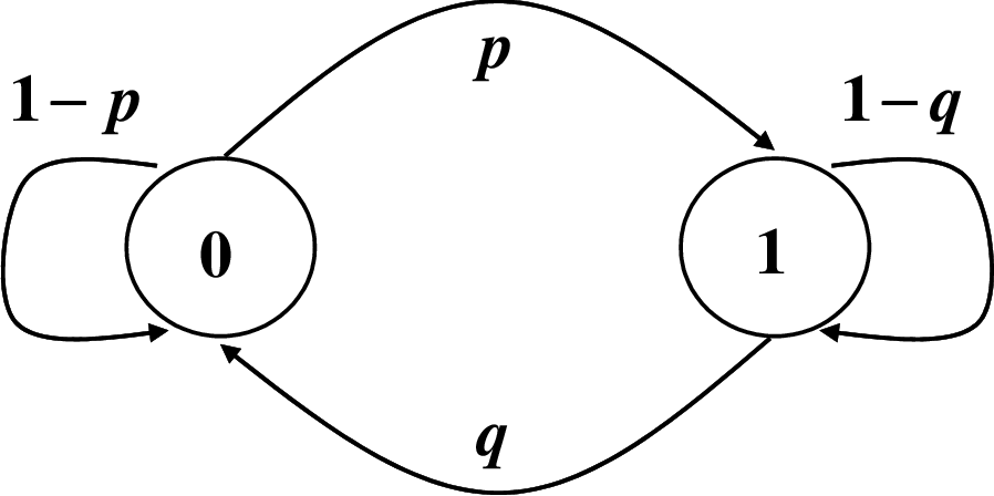
Refer to caption
Fig. 2: The description of the transition matrix.

We consider a binary transition matrix WW given by Fig. 2, i.e.,

W=[1−pqp1−q].\displaystyle W=\left[\begin{array}[]{cc}1-p&q\\ p&1-q\end{array}\right].

In this case, the stationary distribution is

P~​(0)\displaystyle\tilde{P}(0) =\displaystyle= qp+q,\displaystyle\frac{q}{p+q}, (169)
P~​(1)\displaystyle\tilde{P}(1) =\displaystyle= pp+q.\displaystyle\frac{p}{p+q}. (170)

The entropy is

HW​(X)=qp+q​h​(p)+pp+q​h​(q),\displaystyle H^{W}(X)=\frac{q}{p+q}h(p)+\frac{p}{p+q}h(q), (171)

where h⁡(⋅)h(\cdot) is the binary entropy function. The tilted transition matrix is

W~θ=[(1−p)1+θq1+θp1+θ(1−q)1+θ].\displaystyle\tilde{W}_{\theta}=\left[\begin{array}[]{cc}(1-p)^{1+\theta}&q^{1+\theta}\\ p^{1+\theta}&(1-q)^{1+\theta}\end{array}\right].

The Perron-Frobenius eigenvalue is

λθ=\displaystyle\lambda_{\theta}= (1−p)1+θ+(1−q)1+θ2\displaystyle\frac{(1-p)^{1+\theta}+(1-q)^{1+\theta}}{2}
+{(1−p)1+θ−(1−q)1+θ}2+4​p1+θ​q1+θ2\displaystyle+\frac{\sqrt{\{(1-p)^{1+\theta}-(1-q)^{1+\theta}\}^{2}+4p^{1+\theta}q^{1+\theta}}}{2} (175)

and its normalized eigenvector is

P~θ​(0)\displaystyle\tilde{P}_{\theta}(0) =\displaystyle= q1+θλθ−(1−p)1+θ+q1+θ,\displaystyle\frac{q^{1+\theta}}{\lambda_{\theta}-(1-p)^{1+\theta}+q^{1+\theta}}, (176)
P~θ​(1)\displaystyle\tilde{P}_{\theta}(1) =\displaystyle= λθ−(1−p)1+θλθ−(1−p)1+θ+q1+θ.\displaystyle\frac{\lambda_{\theta}-(1-p)^{1+\theta}}{\lambda_{\theta}-(1-p)^{1+\theta}+q^{1+\theta}}. (177)

The eigenvector of W~θT\tilde{W}_{\theta}^{T} satisfying (64) is also given by

vθ​(0)\displaystyle v_{\theta}(0) =\displaystyle= q1+θmin⁡(λθ−(1−p)1+θ,q1+θ),\displaystyle\frac{q^{1+\theta}}{\min(\lambda_{\theta}-(1-p)^{1+\theta},q^{1+\theta})}, (178)
vθ​(1)\displaystyle v_{\theta}(1) =\displaystyle= λθ−(1−p)1+θmin⁡(λθ−(1−p)1+θ,q1+θ).\displaystyle\frac{\lambda_{\theta}-(1-p)^{1+\theta}}{\min(\lambda_{\theta}-(1-p)^{1+\theta},q^{1+\theta})}. (179)

From these calculations, we can evaluate the bounds in Theorems 10, 11, and 12. When the initial distribution is given as PX​(0)=1P_{X}(0)=1 and PX​(1)=0P_{X}(1)=0, for p=0.1p=0.1, q=0.2q=0.2, we plotted the bounds in Fig. 1 for fixed block length n=10000n=10000 and n=1000000n=1000000 and varying ε=Δ⁡(M)\varepsilon=\Delta(M) or Δ¯​(M)\overline{\Delta}(M). The two bounds in Theorems 11 and 12 have similar values in the left of Fig. 1. However, the bound in Theorem 12 has a clear advantage in the right of Fig. 1. That is, to clarify the advantage of Theorem 12, we need a very huge size nn and a very small ϵ\epsilon. Although one may consider that n=1000000n=1000000 is too large to realize, this size is realizable as follows. A typical two-universal hash family can be realized by using Toeplitz matrix. This kind two-universal hash family with n=108n=10^{8} was realized efficiently by using a typical personal computer [10, Appendix B][9].

IV Secure Uniform Random Number Generation

In this section, we investigate the secure random number generation with partial information leakage, which is also known as the privacy amplification. We start this section by showing the problem setting in Section IV-A. Then, we review and introduce some single-shot bounds in Section IV-B. We derive non-asymptotic bounds for the Markov chain in Section IV-C. Then, in Sections IV-D and IV-E, we show the asymptotic characterization for the large deviation regime and the moderate deviation regime by using those non-asymptotic bounds. We also derive the second order rate in Section IV-F.

The results shown in this section are summarized in Table III. The checkmarks ✓\checkmark indicate that the tight asymptotic bounds (large deviation, moderate deviation, and second order) can be obtained from those bounds. The marks ✓∗\checkmark^{*} indicate that the large deviation bound can be derived up to the critical rate. The computational complexity ”Tail” indicates that the computational complexities of those bounds depend on the computational complexities of tail probabilites. It should be noted that Theorem 23 is derived from a special case (QY=PYQ_{Y}=P_{Y}) of Lemma 27. The asymptotically optimal choice is QY=PY(1+θ)Q_{Y}=P_{Y}^{(1+\theta)}, which corresponds to (194) of Lemma 27. Under Assumption 1, we can derive the bound of the Markov case only for that special choice of QYQ_{Y}, while under Assumption 2, we can derive the bound of the Markov case for the optimal choice of QYQ_{Y}. Here, we didn’t call several lemmas as theorems although they derive the asymptotic tight bound. This is because they are not computable form as explained in the beginning of Section III.

IV-A Problem Formulation

The privacy amplification is conducted by a function f:𝒳→{1,…,M}f:{\cal X}\to\{1,\ldots,M\}. The security of the generated key is evaluated by

Δ⁡[f]:=12​‖Pf⁡(X)​Y−PU¯×PY‖1,\displaystyle\Delta[f]:=\frac{1}{2}\|P_{f(X)Y}-P_{\overline{U}}\times P_{Y}\|_{1}, (180)

where U¯\overline{U} is the uniform random variable on {1,…,M}\{1,\ldots,M\} and ∥⋅∥1\|\cdot\|_{1} is the variational distance. For notational convenience, we introduce the infimum of the security criterion under the condition that the range size is MM:

Δ⁡(M):=inffΔ⁡[f].\displaystyle\Delta(M):=\inf_{f}\Delta[f]. (181)

When we construct a function for the privacy amplification, we often use a two-universal hash family ℱ{\cal F} and a random function FF on ℱ{\cal F}. Then, we bound the security criterion averaged over the random function by only using the property of two-universality. As explained in Subsection I-E, to take into the practical aspects, we introduce the worst leaked information:

Δ¯​(M):=supF𝔼⁡[Δ⁡[F]],\displaystyle\overline{\Delta}(M):=\sup_{F}\mathbb{E}[\Delta[F]], (182)

where the supremum is taken over all two-universal hash families from 𝒳{\cal X} to {1,…,M}\{1,\ldots,M\}. From the definition, we obviously have

Δ​(M)≤Δ¯​(M).\displaystyle\Delta(M)\leq\overline{\Delta}(M). (183)

When we consider nn-fold extension, the security criteria are denoted by Δ⁡(Mn)\Delta(M_{n}) or Δ¯​(Mn)\overline{\Delta}(M_{n}). As in the single-terminal case, we also introduce the quantities M⁡(n,ε)M(n,\varepsilon) and M¯​(n,ε)\overline{M}(n,\varepsilon) (cf. (106) and (107)).

Remark 5

Note that the security definition in (180) implies the universal composable security criterion [50, 51]. A slightly weaker security criterion defined by

infQY12​‖Pf⁡(X)​Y−PU¯×QY‖1\displaystyle\inf_{Q_{Y}}\frac{1}{2}\|P_{f(X)Y}-P_{\overline{U}}\times Q_{Y}\|_{1} (184)

also implies the universal composable security criterion. In fact some literatures employs this kinds of security criteria [52, 26, 53]. Since the triangle inequality and the information processing inequality ‖QY−PY‖1≤‖PU¯×QY−Pf⁡(X)​Y‖1\|Q_{Y}-P_{Y}\|_{1}\leq\|P_{\overline{U}}\times Q_{Y}-P_{f(X)Y}\|_{1} imply

12​‖Pf⁡(X)​Y−PU¯×PY‖1\displaystyle\frac{1}{2}\|P_{f(X)Y}-P_{\overline{U}}\times P_{Y}\|_{1}
≤\displaystyle\leq 12​‖Pf⁡(X)​Y−PU¯×QY‖1+12​‖PU¯×QY−PU¯×PY‖1\displaystyle\frac{1}{2}\|P_{f(X)Y}-P_{\overline{U}}\times Q_{Y}\|_{1}+\frac{1}{2}\|P_{\overline{U}}\times Q_{Y}-P_{\overline{U}}\times P_{Y}\|_{1}
=\displaystyle= 12​‖Pf⁡(X)​Y−PU¯×QY‖1+12​‖QY−PY‖1\displaystyle\frac{1}{2}\|P_{f(X)Y}-P_{\overline{U}}\times Q_{Y}\|_{1}+\frac{1}{2}\|Q_{Y}-P_{Y}\|_{1}
≤\displaystyle\leq 12​‖Pf⁡(X)​Y−PU¯×QY‖1+12​‖PU¯×QY−Pf⁡(X)​Y‖1,\displaystyle\frac{1}{2}\|P_{f(X)Y}-P_{\overline{U}}\times Q_{Y}\|_{1}+\frac{1}{2}\|P_{\overline{U}}\times Q_{Y}-P_{f(X)Y}\|_{1},

we have

12​‖Pf⁡(X)​Y−PU¯×PY‖1≤‖Pf⁡(X)​Y−PU¯×QY‖1\displaystyle\frac{1}{2}\|P_{f(X)Y}-P_{\overline{U}}\times P_{Y}\|_{1}\leq\|P_{f(X)Y}-P_{\overline{U}}\times Q_{Y}\|_{1} (185)

holds for any QYQ_{Y}. Thus, the two criteria differ only in constant factor, which means that the asymptotic behaviors of the large deviation regime and the moderate deviation regime are not affected by the choice of the security criteria.

For the second order regime, the same fact can be shown as follows. The achievability part (Lemma 26 given in Subsection IV-B) can be used without modification since the optimization over QYQ_{Y} is already incorporated into the bound. For the converse part, we need to replace Hminε​(PX​Y|PY)H_{\min}^{\varepsilon}(P_{XY}|P_{Y}) with Hminε​(PX​Y|QY)H_{\min}^{\varepsilon}(P_{XY}|Q_{Y}) in Lemma 28 given in Subsection IV-B. Then, the converse bound in Lemma 29 given in Subsection IV-B is modified accordingly, i.e.,

Δ(M)≥infQYmaxγ≥0[PX​Y{logQY​(y)PX​Y​(x,y)<γ}(1−eγM)].\displaystyle\Delta(M)\geq\inf_{Q_{Y}}\max_{\gamma\geq 0}\left[P_{XY}\left\{\log\frac{Q_{Y}(y)}{P_{XY}(x,y)}<\gamma\right\}\left(1-\frac{e^{\gamma}}{M}\right)\right].

However, by noting the inequality

PX​Y{logQY​(y)PX​Y​(x,y)<γ}\displaystyle P_{XY}\left\{\log\frac{Q_{Y}(y)}{P_{XY}(x,y)}<\gamma\right\}
≥\displaystyle\geq PX​Y{log1PX|Y​(x|y)<γ−ν}−PX​Y{logQY​(y)PY​(y)>ν}\displaystyle P_{XY}\left\{\log\frac{1}{P_{X|Y}(x|y)}<\gamma-\nu\right\}-P_{XY}\left\{\log\frac{Q_{Y}(y)}{P_{Y}(y)}>\nu\right\}
≥\displaystyle\geq PX​Y{log1PX|Y​(x|y)<γ−ν}−e−ν\displaystyle P_{XY}\left\{\log\frac{1}{P_{X|Y}(x|y)}<\gamma-\nu\right\}-e^{-\nu} (186)

for any ν>0\nu>0, the choice QY=PYQ_{Y}=P_{Y} turns out to be the optimal choice asymptotically up to o⁡(n)o(\sqrt{n}). Thus, the asymptotic behavior of the second order regime is also not affected by the choice of the security criteria.

When the output size MM is too large, Δ⁡(M)\Delta(M) is close to 11 anymore. In this case, to quantify the performance of the output random number, according to Csiszár-Narayan [29], we focus on the relative entropy between the generated random number and the ideal random number as follows.

D(Pf⁡(X)​Y∥PU¯×PY)=\displaystyle D(P_{f(X)Y}\|P_{\overline{U}}\times P_{Y})= log⁡M−H⁡(f⁡(X)|Y)\displaystyle\log M-H(f(X)|Y)
=\displaystyle= I(f(X);Y)+D(Pf⁡(X)∥PU¯).\displaystyle I(f(X);Y)+D(P_{f(X)}\|P_{\overline{U}}). (187)

Since this quantity can be regarded as a modification of the mutual information I⁡(f⁡(X),Y)I(f(X);Y), we call it the modified mutual information. This quantity is naturally given under axiomatic conditions [28]. Then, we address the following quantities.

D⁡(M):=\displaystyle D(M):= inffD(Pf⁡(X)​Y∥PU¯×PY)\displaystyle\inf_{f}D(P_{f(X)Y}\|P_{\overline{U}}\times P_{Y}) (188)
D¯​(M):=\displaystyle\overline{D}(M):= supF𝔼[D(PF⁡(X)​Y​F∥PU¯×PY)]\displaystyle\sup_{F}\mathbb{E}[D(P_{F(X)YF}\|P_{\overline{U}}\times P_{Y})]
=\displaystyle= D(PF⁡(X)​Y​F∥PU¯×PY×PF)\displaystyle D(P_{F(X)YF}\|P_{\overline{U}}\times P_{Y}\times P_{F}) (189)

where the supremum is taken over all two-universal hash families from 𝒳{\cal X} to {1,…,M}\{1,\ldots,M\}. The reason why we consider such a supremum is the same as the case of Δ¯​(M)\overline{\Delta}(M).

IV-B Single Shot Bounds

In this section, we review existing single shot bounds, and show a novel converse bound. For the information measures used below, see Section II. We also introduce the following information measures. For PX​Y∈𝒫¯​(𝒳×𝒴)P_{XY}\in\overline{{\cal P}}({\cal X}\times{\cal Y}) and QY∈𝒫⁡(𝒴)Q_{Y}\in{\cal P}({\cal Y})1414 14 Technically, we restrict QYQ_{Y} to be such that supp⁡(PY)⊂supp⁡(QY)\mathrm{supp}(P_{Y})\subset\mathrm{supp}(Q_{Y})., let

Hmin​(PX​Y|QY):=−log⁡maxx,y⁡PX​Y​(x,y)QY​(y)\displaystyle H_{\min}(P_{XY}|Q_{Y}):=-\log\max_{x,y}\frac{P_{XY}(x,y)}{Q_{Y}(y)} (190)

be the conditional min\min-entropy. Then, for PX​Y∈𝒫⁡(𝒳×𝒴)P_{XY}\in{\cal P}({\cal X}\times{\cal Y}), let

Hminε​(PX​Y|QY):=maxPX​Y′∈ℬε​(PX​Y)⁡Hmin​(PX​Y′|QY)\displaystyle H_{\min}^{\varepsilon}(P_{XY}|Q_{Y}):=\max_{P^{\prime}_{XY}\in{\cal B}^{\varepsilon}(P_{XY})}H_{\min}(P^{\prime}_{XY}|Q_{Y}) (191)

and

H¯minε​(PX​Y|QY):=maxPX​Y′∈ℬ¯ε​(PX​Y)⁡Hmin​(PX​Y′|QY)\displaystyle\overline{H}_{\min}^{\varepsilon}(P_{XY}|Q_{Y}):=\max_{P^{\prime}_{XY}\in\overline{{\cal B}}^{\varepsilon}(P_{XY})}H_{\min}(P^{\prime}_{XY}|Q_{Y}) (192)

be the smooth min\min-entropy, where

ℬ⁡(PX​Y):=\displaystyle{\cal B}(P_{XY}):= {PX​Y′∈𝒫⁡(𝒳×𝒴):12​‖PX​Y−PX​Y′‖1≤ε},\displaystyle\left\{P^{\prime}_{XY}\in{\cal P}({\cal X}\times{\cal Y}):\frac{1}{2}\|P_{XY}-P^{\prime}_{XY}\|_{1}\leq\varepsilon\right\},
ℬ¯​(PX​Y):=\displaystyle\overline{{\cal B}}(P_{XY}):= {PX​Y′∈𝒫¯​(𝒳×𝒴):12​‖PX​Y−PX​Y′‖1≤ε}.\displaystyle\left\{P^{\prime}_{XY}\in\overline{{\cal P}}({\cal X}\times{\cal Y}):\frac{1}{2}\|P_{XY}-P^{\prime}_{XY}\|_{1}\leq\varepsilon\right\}.

By using the two-universal hash family, we can derive the following bound.

Lemma 25 ([25])

For any QY∈𝒫⁡(𝒴)Q_{Y}\in{\cal P}({\cal Y}), we have

Δ¯​(M)≤2​ε+12​M​e−H¯minε​(PX​Y|QY).\displaystyle\overline{\Delta}(M)\leq 2\varepsilon+\frac{1}{2}\sqrt{Me^{-\overline{H}_{\min}^{\varepsilon}(P_{XY}|Q_{Y})}}.

However, the bound in Lemma 25 cannot be directly calculated in the Markovian chain. To resolve this problem, we slightly loosen Lemma 25 as follows. (cf. [28, Theorem 23] or [27, Lemma 3]).

Lemma 26

For any QY∈𝒫⁡(𝒴)Q_{Y}\in{\cal P}({\cal Y}), we have

Δ¯(M)≤infγ≥0[PX​Y{logQY​(y)PX​Y​(x,y)<γ}+12Meγ].\displaystyle\overline{\Delta}(M)\leq\inf_{\gamma\geq 0}\left[P_{XY}\left\{\log\frac{Q_{Y}(y)}{P_{XY}(x,y)}<\gamma\right\}+\frac{1}{2}\sqrt{\frac{M}{e^{\gamma}}}\right].

We also have the following exponential bound.

Lemma 27 ([12])

We have

Δ¯​(M)\displaystyle\overline{\Delta}(M)
≤\displaystyle\leq min⁡inf0≤θ≤1QY∈𝒫⁡(𝒴)⁡32​Mθ1+θ​e−θ1+θ​H1+θ​(PX​Y|QY)\displaystyle\min_{Q_{Y}\in{\cal P}({\cal Y})}\inf_{0\leq\theta\leq 1}\frac{3}{2}M^{\frac{\theta}{1+\theta}}e^{-\frac{\theta}{1+\theta}H_{1+\theta}(P_{XY}|Q_{Y})} (193)
=\displaystyle= inf0≤θ≤132​Mθ1+θ​e−θ1+θ​H1+θ↑​(X|Y).\displaystyle\inf_{0\leq\theta\leq 1}\frac{3}{2}M^{\frac{\theta}{1+\theta}}e^{-\frac{\theta}{1+\theta}H_{1+\theta}^{\uparrow}(X|Y)}. (194)

For the converse bound, the following is known1515 15 See also [27] for a proof that is specialized for the classical case..

Lemma 28 ([25])

We have

Δ⁡(M)≥minHminε​(PX​Y|PY)≥log⁡M⁡ε.\displaystyle\Delta(M)\geq\min_{H_{\min}^{\varepsilon}(P_{XY}|P_{Y})\geq\log M}\varepsilon. (195)

Similar to Lemma 25, the bound in Lemma 28 cannot be directly calculated in the Markovian chain. To resolve this problem, we slightly loosen Lemma 28 as follows.

Lemma 29

We have

Δ(M)≥maxγ≥0[PX​Y{log1PX|Y​(x|y)<γ}(1−eγM)].\displaystyle\Delta(M)\geq\max_{\gamma\geq 0}\left[P_{XY}\left\{\log\frac{1}{P_{X|Y}(x|y)}<\gamma\right\}\left(1-\frac{e^{\gamma}}{M}\right)\right]. (196)
Proof.

The proof is exactly the same as Lemma 21. ∎

Although Lemma 29 is useful for the large deviation regime and the moderate deviation regime, it is not useful for the second order regime. To resolve this problem, we loosen Lemma 29 as follows.

Lemma 30

We have

Δ(M)≥supγ≥0[PX​Y{log1PX|Y​(x|y)<γ}−eγM].\displaystyle\Delta(M)\geq\sup_{\gamma\geq 0}\left[P_{XY}\left\{\log\frac{1}{P_{X|Y}(x|y)}<\gamma\right\}-\frac{e^{\gamma}}{M}\right]. (197)

Furthermore, by using a property of the strong universal hash family, we can derive the following converse as a generalization of Lemma 23.

Lemma 31

For {Ωy}y∈𝒴\{\Omega_{y}\}_{y\in{\cal Y}} such that |Ωy|≤N≤M|\Omega_{y}|\leq N\leq M for every y∈𝒴y\in{\cal Y}, let Ω=∪y∈𝒴Ωy×{y}\Omega=\cup_{y\in{\cal Y}}\Omega_{y}\times\{y\}. Then, we have

Δ¯​(M)≥(1−NM)2​PX​Y​(Ω).\displaystyle\overline{\Delta}(M)\geq\left(1-\frac{N}{M}\right)^{2}P_{XY}(\Omega). (198)
Proof.

We apply Lemma 23 to each PX|Y(⋅|y)P_{X|Y}(\cdot|y) and take average over yy. Then, we can derive the lemma since |Ωy|≤N|\Omega_{y}|\leq N by the assumption. ∎

Similar to Lemmas 25 and 28, the bound in Lemma 31 cannot be directly calculated in the Markovian chain. To resolve this problem, we slightly loosen Lemma 31 as follows.

Lemma 32

For any 0<ν<10<\nu<1, we have

Δ¯(M)≥(1−ν)2PX​Y{logPY(1+θ⁡(a⁡(R)))​(y)PX​Y​(x,y)≤a(R)},\displaystyle\overline{\Delta}(M)\geq(1-\nu)^{2}P_{XY}\left\{\log\frac{P_{Y}^{(1+\theta(a(R)))}(y)}{P_{XY}(x,y)}\leq a(R)\right\}, (199)

where R=log⁡(M​ν)R=\log(M\nu), and θ⁡(a)\theta(a) and a⁡(R)a(R) are the inverse functions θ↑​(a)\theta^{\uparrow}(a) and a↑​(R)a^{\uparrow}(R) defined by (20) and (21) respectively.

Proof.

See Appendix H. ∎

To derive a converse bound for Δ⁡(M){\Delta}(M) based on the conditional Rényi entropy, we substitute the formula in Proposition 3 in Appendix A into the bound in Lemma 29 for a=γ=log⁡(M/2)a=\gamma=\log(M/2). So, we have the following.

Theorem 20

We have

−log⁡Δ⁡(M)\displaystyle-\log\Delta(M)
≤\displaystyle\leq infs>0θ~>θ⁡(a)1s[(1+s)θ~(H1+θ~↓(X|Y)−H1+(1+s)​θ~↓(X|Y))\displaystyle\inf_{s>0\atop\tilde{\theta}>\theta(a)}\frac{1}{s}\Bigg[(1+s)\tilde{\theta}\bigg(H_{1+\tilde{\theta}}^{\downarrow}(X|Y)-H_{1+(1+s)\tilde{\theta}}^{\downarrow}(X|Y)\bigg)
−(1+s)​log⁡(1CLOSE\displaystyle\hskip 12.91663pt-(1+s)\log\bigg(1
−e(θ⁡(a)−θ~)​a−θ⁡(a)​H1+θ⁡(a)↓​(X|Y)+θ~​H1+θ~↓​(X|Y))]\displaystyle\hskip 38.74988pt-e^{(\theta(a)-\tilde{\theta})a-\theta(a)H_{1+\theta(a)}^{\downarrow}(X|Y)+\tilde{\theta}H_{1+\tilde{\theta}}^{\downarrow}(X|Y)}\bigg)\Bigg]
+log⁡2,\displaystyle+\log 2, (200)

where a=log⁡(M/2)a=\log(M/2), and θ⁡(a)\theta(a) is the inverse function θ↓​(a)\theta^{\downarrow}(a) defined by (18).

Proof.

Theorem 20 can be shown by the same way as Theorem 11 with replacing the role of Lemma 21 by Lemma 20. ∎

To derive a converse bound for Δ¯​(M)\overline{\Delta}(M) based on the conditional Rényi entropy, we substitute the formula in Proposition 3 in Appendix A into the bound in Lemma 21 for ν=12\nu=\frac{1}{2}. So, we have the following.

Theorem 21

We have

−log⁡Δ¯​(M)\displaystyle-\log\overline{\Delta}(M)
≤\displaystyle\leq infs>0θ~>θ⁡(a⁡(R))1s[(1+s)θ~(H1+θ~,1+θ⁡(a⁡(R))(X|Y)\displaystyle\inf_{s>0\atop\tilde{\theta}>\theta(a(R))}\frac{1}{s}\bigg[(1+s)\tilde{\theta}\bigg(H_{1+\tilde{\theta},1+\theta(a(R))}(X|Y)
−H1+(1+s)​θ~,1+θ⁡(a⁡(R))(X|Y))−(1+s)log(1−eC2,n)]\displaystyle-H_{1+(1+s)\tilde{\theta},1+\theta(a(R))}(X|Y)\bigg)-(1+s)\log\left(1-e^{C_{2,n}}\right)\bigg]
+2​log⁡2,\displaystyle+2\log 2, (201)

where R=log⁡(M/2)R=\log(M/2),

C2,n:=\displaystyle C_{2,n}:= [θ⁡(a⁡(R))−θ~]​a​(R)−θ⁡(a⁡(R))​H1+θ⁡(a⁡(R))↑​(X|Y)\displaystyle[\theta(a(R))-\tilde{\theta}]a(R)-\theta(a(R))H_{1+\theta(a(R))}^{\uparrow}(X|Y)
+θ~​H1+θ~,1+θ⁡(a⁡(R))​(X|Y),\displaystyle+\tilde{\theta}H_{1+\tilde{\theta},1+\theta(a(R))}(X|Y),

and θ⁡(a)\theta(a) and a⁡(R)a(R) are the inverse functions θ↑​(a)\theta^{\uparrow}(a) and a↑​(R)a^{\uparrow}(R) defined by (20) and (21) respectively.

Proof.

Theorem 21 can be shown by the same way as Theorem 8 with replacing the role of Lemma 24 by Lemma 32. ∎

Finally, we address the modified mutual information rate (MMIR). As the direct part, we have the following theorem.

Theorem 22

The maximum modified mutual information D¯​(M)\overline{D}(M) among two-universal hash family is bounded as

D¯​(M)≤1θ​log⁡(1+Mθ​e−θ​H1+θ​(X|Y)).\displaystyle\overline{D}(M)\leq\frac{1}{\theta}\log(1+M^{\theta}e^{-\theta H_{1+\theta}(X|Y)}). (202)
Proof.

Lemma 10 of [47] shows that any two-universal hash function FF satisfies the relation

𝔼⁡(Mθ​e−θ​H1+θ​(F⁡(X|Y)))≤1+Mθ​e−θ​H1+θ​(X|Y),\displaystyle\mathbb{E}(M^{\theta}e^{-\theta H_{1+\theta}(F(X|Y))})\leq 1+M^{\theta}e^{-\theta H_{1+\theta}(X|Y)}, (203)

which implies that 𝔼⁡[log⁡M−H⁡(F⁡(X|Y))]≤𝔼⁡[log⁡M−H1+s​(F⁡(X)|Y)]≤1s​log⁡𝔼⁡(Ms​e−s​H1+s​(F⁡(X)|Y))≤1s​log⁡(1+Ms​e−s​H1+s​(X|Y))\mathbb{E}[\log M-H(F(X|Y))]\leq\mathbb{E}[\log M-H_{1+s}(F(X)|Y)]\leq\frac{1}{s}\log\mathbb{E}(M^{s}e^{-sH_{1+s}(F(X)|Y)})\leq\frac{1}{s}\log(1+M^{s}e^{-sH_{1+s}(X|Y)}). ∎

As the converse part, we have the following theorem.

Proposition 2
D⁡(M)≥log⁡M−H⁡(PX)\displaystyle D(M)\geq\log M-H(P_{X}) (204)
Proof.

Inequality (204) follows from the inequality H⁡(X|Y)≥H⁡(f⁡(X)|Y)H(X|Y)\geq H(f(X)|Y). ∎

IV-C Finite-Length Bounds for Markov Source

Since we assume the irreducibility for the transition matrix describing the Markovian chain, the following bounds hold with any initial distribution. To lower bound −log⁡Δ¯​(Mn)-\log\overline{\Delta}(M_{n}) by the lower conditional Rényi entropy of transition matrix, we substitute the formula for the lower conditional Rényi entropy given in Lemma 8 into the bound in Lemma 27 for QYn=PYnQ_{Y^{n}}=P_{Y^{n}}, we have the following achievability bound.

Theorem 23

Suppose that a transition matrix WW satisfies Assumption 1. Let R:=1n​log⁡MnR:=\frac{1}{n}\log M_{n}. Then we have

−log⁡Δ¯​(Mn)\displaystyle-\log\overline{\Delta}(M_{n})
≥\displaystyle\geq sup0≤θ≤1−θ​n​R+(n−1)​θ​H1+θ↓,W​(X|Y)+δ¯​(θ)1+θ−log⁡(3/2).\displaystyle\sup_{0\leq\theta\leq 1}\frac{-\theta nR+(n-1)\theta H_{1+\theta}^{\downarrow,W}(X|Y)+\underline{\delta}(\theta)}{1+\theta}-\log(3/2). (205)

To upper bound −log⁡Δ⁡(Mn)-\log{\Delta}(M_{n}) by the lower conditional Rényi entropy of transition matrix, we substitute the formula for the tail probability given in and Proposition 4 with a=Ra=R into the bound in Lemma 29 with γ=n​R\gamma=nR, we have the following converse bound.

Theorem 24

Suppose that a transition matrix WW satisfies Assumption 1. Let R:=1n​log⁡(Mn/2)R:=\frac{1}{n}\log(M_{n}/2). For any a¯<R<HW​(X|Y)\underline{a}<R<H^{W}(X|Y), we have

−log⁡Δ⁡(Mn)\displaystyle-\log\Delta(M_{n})
≤\displaystyle\leq infs>0θ~>θ⁡(a)1s[(n−1)(1+s)θ~(H1+θ~↓,W(X|Y)\displaystyle\inf_{s>0\atop\tilde{\theta}>\theta(a)}\frac{1}{s}\Bigg[(n-1)(1+s)\tilde{\theta}\bigg(H_{1+\tilde{\theta}}^{\downarrow,W}(X|Y)
−H1+(1+s)​θ~↓,W(X|Y))+δ1−(1+s)log(1−eC3,n)]\displaystyle-H_{1+(1+s)\tilde{\theta}}^{\downarrow,W}(X|Y)\bigg)+\delta_{1}-(1+s)\log\left(1-e^{C_{3,n}}\right)\Bigg]
+log⁡2,\displaystyle+\log 2, (206)

where θ⁡(a)\theta(a) is the inverse function θ↓​(a)\theta^{\downarrow}(a) defined by (46), and

C3,n:=\displaystyle C_{3,n}:= (n−1)​((θ⁡(R)−θ~)​R−θ⁡(R)​H1+θ⁡(R)↓,W​(X|Y)CLOSE\displaystyle(n-1)\bigg((\theta(R)-\tilde{\theta})R-\theta(R)H_{1+\theta(R)}^{\downarrow,W}(X|Y)
OPEN+θ~​H1+θ~↓,W​(X|Y))+δ2,\displaystyle\hskip 43.05542pt+\tilde{\theta}H_{1+\tilde{\theta}}^{\downarrow,W}(X|Y)\bigg)+\delta_{2}, (207)
δ1:=\displaystyle\delta_{1}:= (1+s)​δ¯​(θ~)−δ¯​((1+s)​θ~),\displaystyle(1+s)\overline{\delta}(\tilde{\theta})-\underline{\delta}((1+s)\tilde{\theta}), (208)
δ2:=\displaystyle\delta_{2}:= (θ⁡(R)−θ~)​R−δ¯​(θ⁡(R))+δ¯​(θ~).\displaystyle(\theta(R)-\tilde{\theta})R-\underline{\delta}(\theta(R))+\overline{\delta}(\tilde{\theta}). (209)
Proof.

Theorem 24 can be shown by the same way as Theorem 11 with replacing the roles of Lemma 21 and Proposition 3 in Appendix A by Lemma 20 and Proposition 4. ∎

Next, we derive tighter bounds under Assumption 2. To lower bound −log⁡Δ¯​(Mn)-\log\overline{\Delta}(M_{n}) by the upper conditional Rényi entropy of transition matrix, we substitute the formula for the upper conditional Rényi entropy given in Lemma 9 into the bound in Lemma 27, we have the following achievability bound.

Theorem 25

Suppose that a transition matrix WW satisfies Assumption 2. Let R:=1n​log⁡MnR:=\frac{1}{n}\log M_{n}. Then we have

−log⁡Δ¯​(Mn)\displaystyle-\log\overline{\Delta}(M_{n})
≥\displaystyle\geq sup0≤θ≤1−θ​n​R+(n−1)​θ​H1+θ↑,W​(X|Y)1+θ+ξ¯​(θ)−log⁡(3/2).\displaystyle\sup_{0\leq\theta\leq 1}\frac{-\theta nR+(n-1)\theta H_{1+\theta}^{\uparrow,W}(X|Y)}{1+\theta}+\underline{\xi}(\theta)-\log(3/2). (210)

To upper bound −log⁡Δ⁡(Mn)-\log{\Delta}(M_{n}) by the upper conditional Rényi entropy of transition matrix, we substitute the formula for the tail probability given in and Proposition 3 in Appendix A into the bound in Lemma 311616 16 We cannot apply Proposition 4 here since we cannot apply Lemma 34 for ϕ⁡(ρ~;PXn​Yn|QYn(1−ρ))\phi(\tilde{\rho};P_{X^{n}Y^{n}}|Q_{Y^{n}}^{(1-\rho)}). Instead, we need to apply Lemma 10., we have the following converse bound.

Theorem 26

Suppose that a transition matrix WW satisfies Assumption 2. Let RR be such that

(n−1)​R+((1+θ⁡(a⁡(R)))​(a⁡(R)−ξ¯​(θ⁡(a⁡(R)))))\displaystyle(n-1)R+\Bigg((1+\theta(a(R)))(a(R)-\underline{\xi}(\theta(a(R))))\Bigg)
=\displaystyle= log⁡(Mn/2).\displaystyle\log(M_{n}/2). (211)

If R⁡(a¯)<R<HW​(X|Y)R(\underline{a})<R<H^{W}(X|Y), then we have

−log⁡Δ¯​(Mn)\displaystyle-\log\overline{\Delta}(M_{n})
≤\displaystyle\leq infs>0θ~>θ⁡(a⁡(R))1s[(n−1)(1+s)θ~(H1+θ~,1+θ⁡(a⁡(R))W(X|Y)\displaystyle\inf_{s>0\atop\tilde{\theta}>\theta(a(R))}\frac{1}{s}\Bigg[(n-1)(1+s)\tilde{\theta}\bigg(H_{1+\tilde{\theta},1+\theta(a(R))}^{W}(X|Y)
OPEN−H1+(1+s)​θ~,1+θ⁡(a⁡(R))W​(X|Y))+δ1\displaystyle\hskip 47.36096pt-H_{1+(1+s)\tilde{\theta},1+\theta(a(R))}^{W}(X|Y)\bigg)+\delta_{1}
−(1+s)log(1−eC4,n)]+2log2,\displaystyle\hskip 47.36096pt-(1+s)\log\left(1-e^{C_{4,n}}\right)\Bigg]+2\log 2, (212)

where θ⁡(a)\theta(a) and a⁡(R)a(R) are the inverse functions θ↑​(a)\theta^{\uparrow}(a) and a↑​(R)a^{\uparrow}(R) defined by (56) and (58) respectively,

C4,n:=\displaystyle C_{4,n}:= (n−1)[(θ(a(R))−θ~)(a(R))\displaystyle(n-1)\Big[(\theta(a(R))-\tilde{\theta})(a(R))
−θ⁡(a⁡(R))​H1+θ⁡(a⁡(R))↑,W​(X|Y)\displaystyle\hskip 34.44434pt-\theta(a(R))H_{1+\theta(a(R))}^{\uparrow,W}(X|Y)
+θ~H1+θ~,1+θ⁡(a⁡(R))W(X|Y)]+δ2\displaystyle\hskip 47.36096pt+\tilde{\theta}H_{1+\tilde{\theta},1+\theta(a(R))}^{W}(X|Y)\Big]+\delta_{2} (213)
δ1:=\displaystyle\delta_{1}:= (1+s)​ζ¯​(θ~,θ⁡(a⁡(R)))−ζ¯​((1+s)​θ~,θ⁡(a⁡(R))),\displaystyle(1+s)\overline{\zeta}(\tilde{\theta},\theta(a(R)))-\underline{\zeta}((1+s)\tilde{\theta},\theta(a(R))), (214)
δ2:=\displaystyle\delta_{2}:= (θ⁡(a⁡(R))−θ~)​(a⁡(R))−ζ¯​(θ⁡(a⁡(R)),θ⁡(a⁡(R)))\displaystyle(\theta(a(R))-\tilde{\theta})(a(R))-\underline{\zeta}(\theta(a(R)),\theta(a(R)))
+ζ¯​(θ~,θ​(a​(R))).\displaystyle+\overline{\zeta}(\tilde{\theta},\theta(a(R))). (215)
Proof.

See Appendix I. ∎

We derive finite-length bounds for modified mutual information rate under Assumption 1 by substituting the formula for the lower conditional Rényi entropy given in Lemma 8 into the bound in Theorem 22.

Theorem 27

When R−H1+θ↓,W​(X|Y)≥0R-H_{1+\theta}^{\downarrow,W}(X|Y)\geq 0, for θ∈[0,1]\theta\in[0,1], we have

OPENOPEND¯​(en​R)≤n​R−(n−1)​H1+θ↓,W​(X|Y))+1θ​(log⁡2−δ¯​(θ))).\displaystyle\overline{D}(e^{nR})\leq nR-(n-1)H^{\downarrow,W}_{1+\theta}(X|Y))+\frac{1}{\theta}(\log 2-\underline{\delta}(\theta))). (216)
Proof.

Theorem 27 can be shown as the same way as Theorem 13 by replacing H1+θW​(X)H^{W}_{1+\theta}(X) and Theorem 9 by H1+θ↓,W​(X|Y)H^{\downarrow,W}_{1+\theta}(X|Y) and Theorem 22, respectively. ∎

To lower bound D¯​(en​R)\overline{D}(e^{nR}) by the lower conditional Rényi entropy of transition matrix, we substitute the other formula for the lower conditional Rényi entropy given in Lemma 8 into the bound in Proposition 2, we have the following bound.

Theorem 28

For θ∈[0,1]\theta\in[0,1], we have

D⁡(en​R)≥n​R−(n−1)​H1−θ↓,W​(X)+δ¯​(−θ)θ\displaystyle D(e^{nR})\geq nR-(n-1)H^{\downarrow,W}_{1-\theta}(X)+\frac{\underline{\delta}(-\theta)}{\theta} (217)
Proof.

Theorem 28 can be shown as the same way as Theorem 14 by replacing H1−θW​(X)H^{W}_{1-\theta}(X) and Proposition 1 by H1−θ↓,W​(X|Y)H^{\downarrow,W}_{1-\theta}(X|Y) and Proposition 2, respectively. ∎

IV-D Large Deviation

We can show the following theorem in the same way as Theorem 15 by taking the limit in Theorems 23 and 24 with use of Lemma 6.

Theorem 29

Suppose that a transition matrix WW satisfies Assumption 1. For R<HW​(X|Y)R<H^{W}(X|Y), we have

lim infn→∞−1nlogΔ¯(en​R)≥sup0≤θ≤1−θ​R+θ​H1+θ↓,W​(X|Y)1+θ.\displaystyle\liminf_{n\to\infty}-\frac{1}{n}\log\overline{\Delta}\left(e^{nR}\right)\geq\sup_{0\leq\theta\leq 1}\frac{-\theta R+\theta H_{1+\theta}^{\downarrow,W}(X|Y)}{1+\theta}. (218)

On the other hand, for a¯<R<HW​(X|Y)\underline{a}<R<H^{W}(X|Y), we have

lim supn→∞−1nlogΔ(en​R)\displaystyle\limsup_{n\to\infty}-\frac{1}{n}\log\Delta\left(e^{nR}\right)
≤\displaystyle\leq −θ⁡(R)​R+θ⁡(R)​H1+θ⁡(R)↓,W​(X|Y)\displaystyle-\theta(R)R+\theta(R)H_{1+\theta(R)}^{\downarrow,W}(X|Y) (219)
=\displaystyle= sup0≤θ−θR+θH1+θ↓,W(X|Y),\displaystyle\sup_{0\leq\theta}-\theta R+\theta H_{1+\theta}^{\downarrow,W}(X|Y), (220)

where θ⁡(a)\theta(a) is the inverse function θ↓​(a)\theta^{\downarrow}(a) defined by (46).

Under Assumption 2, taking the limit in Theorems 25 and 26, we have the following tighter bound.

Theorem 30

Suppose that a transition matrix WW satisfies Assumption 2. For R<HW​(X|Y)R<H^{W}(X|Y), we have

lim infn→∞−1nlogΔ¯(en​R)≥sup0≤θ≤1−θ​R+θ​H1+θ↑,W​(X|Y)1+θ.\displaystyle\liminf_{n\to\infty}-\frac{1}{n}\log\overline{\Delta}\left(e^{nR}\right)\geq\sup_{0\leq\theta\leq 1}\frac{-\theta R+\theta H_{1+\theta}^{\uparrow,W}(X|Y)}{1+\theta}. (221)

On the other hand, for R⁡(a¯)<R<HW​(X|Y)R(\underline{a})<R<H^{W}(X|Y), we have

lim supn→∞−1nlogΔ¯(en​R)\displaystyle\limsup_{n\to\infty}-\frac{1}{n}\log\overline{\Delta}\left(e^{nR}\right)
≤\displaystyle\leq −θ⁡(a⁡(R))​a​(R)+θ⁡(a⁡(R))​H1+θ⁡(a⁡(R))↑,W​(X|Y)\displaystyle-\theta(a(R))a(R)+\theta(a(R))H_{1+\theta(a(R))}^{\uparrow,W}(X|Y) (222)
=\displaystyle= sup0≤θ−θ​R+θ​H1+θ↑,W​(X|Y)1+θ,\displaystyle\sup_{0\leq\theta}\frac{-\theta R+\theta H_{1+\theta}^{\uparrow,W}(X|Y)}{1+\theta}, (223)

where θ⁡(a)\theta(a) and a⁡(R)a(R) are the inverse functions θ↑​(a)\theta^{\uparrow}(a) and a↑​(R)a^{\uparrow}(R) defined by (56) and (58) respectively.

Due to Lemma 7, the lower bound (221) and the upper bound (222) coincide when RR is not less than the critical rate RcrR_{\mathrm{cr}}.

Proof.

(210) in Theorem 25 yields (221). Lemma 7 guarantees (223). So, we will prove (222).

We fix s>0s>0 and θ~>θ⁡(a⁡(R))\tilde{\theta}>\theta(a(R)). Then, (212) implies that

limn→∞−1nlogΔ¯(Mn)\displaystyle\lim_{n\to\infty}-\frac{1}{n}\log\overline{\Delta}(M_{n})
≤\displaystyle\leq +ss​θ~​(H1+θ~,1+θ⁡(a⁡(R))W​(X|Y)−H1+(1+s)​θ~,1+θ⁡(a⁡(R))W​(X|Y))\displaystyle\!\frac{1\!+\!s}{s}\!\tilde{\theta}\Biggl(H_{1+\tilde{\theta},1+\theta(a(R))}^{W}(X|Y)\!-\!H_{1+(1+s)\tilde{\theta},1+\theta(a(R))}^{W}(X|Y)\Biggr) (224)

Similar to (152), taking the limits s→0s\to 0 and θ~→θ⁡(a⁡(R))\tilde{\theta}\to\theta(a(R)), we have

1+ss​θ~​(H1+θ~,1+θ⁡(a⁡(R))W​(X|Y)CLOSE\displaystyle\frac{1+s}{s}\tilde{\theta}\Bigg(H_{1+\tilde{\theta},1+\theta(a(R))}^{W}(X|Y)
OPEN−H1+(1+s)​θ~,1+θ⁡(a⁡(R))W​(X|Y))\displaystyle\hskip 81.8053pt-H_{1+(1+s)\tilde{\theta},1+\theta(a(R))}^{W}(X|Y)\Bigg)
→\displaystyle\to −θ~​d​θ​H1+θ,1+θ⁡(a⁡(R))W​(X|Y)d​θ|θ=θ~\displaystyle-\tilde{\theta}\frac{d{\theta}H_{1+{\theta},1+\theta(a(R))}^{W}(X|Y)}{d\theta}\biggl|_{\theta=\tilde{\theta}}
+θ~​H1+θ~,1+θ⁡(a⁡(R))W​(X|Y)(as s→0)\displaystyle\hskip 64.58313pt+\tilde{\theta}H_{1+\tilde{\theta},1+\theta(a(R))}^{W}(X|Y)\quad\hbox{(as $s\to 0$)}
→\displaystyle\to −θ⁡(a⁡(R))​d​θ​H1+θ,1+θ⁡(a⁡(R))W​(X|Y)d​θ|θ=θ⁡(a⁡(R))\displaystyle-\theta(a(R))\frac{d{\theta}H_{1+{\theta},1+\theta(a(R))}^{W}(X|Y)}{d\theta}\biggl|_{\theta=\theta(a(R))}
+θ⁡(a⁡(R))​H1+θ⁡(a⁡(R))↑,W​(X|Y)(as θ~→θ⁡(a⁡(R)))\displaystyle\hskip 34.44434pt+\theta(a(R))H_{1+\theta(a(R))}^{\uparrow,W}(X|Y)\quad\hbox{(as $\tilde{\theta}\to\theta(a(R))$)}
=(a)\displaystyle\stackrel{{\scriptstyle(a)}}{{=}} θ⁡(a⁡(R))​a+θ⁡(a⁡(R))​H1+θ⁡(a⁡(R))↑,W​(X|Y).\displaystyle\theta(a(R))a+\theta(a(R))H_{1+\theta(a(R))}^{\uparrow,W}(X|Y). (225)

where (a)(a) follows from (56). Hence, (225) and (224) imply that

limn→∞−1nlogΔ¯(Mn)≤θ(a(R))a+θ(a(R))H1+θ⁡(a⁡(R))↑,W(X|Y),\displaystyle\lim_{n\to\infty}-\frac{1}{n}\log\overline{\Delta}(M_{n})\leq\theta(a(R))a+\theta(a(R))H_{1+\theta(a(R))}^{\uparrow,W}(X|Y), (226)

which implies (222). ∎

IV-E Moderate Deviation

Taking the limit with R=HW​(X|Y)−n−t​δR=H^{W}(X|Y)-n^{-t}\delta in Theorem 23 and Theorem 24, we have the following.

Theorem 31

Suppose that a transition matrix WW satisfies Assumption 1. For arbitrary t∈(0,1/2)t\in(0,1/2) and δ>0\delta>0, we have

limn→∞−1n1−2​tlogΔ(en​HW​(X|Y)−n1−t​δ)\displaystyle\lim_{n\to\infty}-\frac{1}{n^{1-2t}}\log\Delta\left(e^{nH^{W}(X|Y)-n^{1-t}\delta}\right)
=\displaystyle= limn→∞−1n1−2​tlogΔ¯(en​HW​(X|Y)−n1−t​δ)=δ22​𝖵W​(X|Y).\displaystyle\lim_{n\to\infty}-\frac{1}{n^{1-2t}}\log\overline{\Delta}\left(e^{nH^{W}(X|Y)-n^{1-t}\delta}\right)=\frac{\delta^{2}}{2\mathsf{V}^{W}(X|Y)}. (227)
Proof.

This theorem can be shown by the same way as Theorem 17 by replacing (138) and (139) by (205) and (206), respectively. ∎

IV-F Second Order

By applying the central limit theorem to Lemmas 26 and 30, and by using Theorem 2, we have the following.

Theorem 32

Suppose that a transition matrix WW satisfies Assumption 1. For arbitrary ε∈(0,1)\varepsilon\in(0,1), we have

limn→∞log⁡M⁡(n,ε)−n​HW​(X|Y)n\displaystyle\lim_{n\to\infty}\frac{\log M(n,\varepsilon)-nH^{W}(X|Y)}{\sqrt{n}}
=\displaystyle= limn→∞log⁡M¯​(n,ε)−n​HW​(X|Y)n\displaystyle\lim_{n\to\infty}\frac{\log\overline{M}(n,\varepsilon)-nH^{W}(X|Y)}{\sqrt{n}}
=\displaystyle= 𝖵W​(X|Y)​Φ−1​(ε).\displaystyle\sqrt{\mathsf{V}^{W}(X|Y)}\Phi^{-1}(\varepsilon). (228)
Proof.

The central limit theorem for Markovian process [41, 48, 49] [35, Corollary 6.2.] guarantees that the random variable (log⁡PXn|Yn​(Xn|Yn)−n​HW​(X|Y))/n(\log P_{X^{n}|Y^{n}}(X^{n}|Y^{n})-nH^{W}(X|Y))/\sqrt{n} asymptotically obeys the normal distribution with the average 00 and the variance 𝖵W​(X|Y)\mathsf{V}^{W}(X|Y). This theorem can be shown by the same way as Theorem 18 by replacing the roles of Lemmas 18 and 22 by those of Lemmas 26 and 30 with QY=PYQ_{Y}=P_{Y}, respectively. ∎

IV-G Modified Mutual Information Rate (MMIR)

Taking the limit in Theorems 27 and 28, we have the following.

Theorem 33

Suppose that a transition matrix WW satisfies Assumption 1. The modified mutual information rate (MMIR) is asymptotically calculated as

limn→∞1n​D​(en​R)=limn→∞1n​D¯​(en​R)=[R−HW​(X|Y)]+.\displaystyle\lim_{n\to\infty}\frac{1}{n}D(e^{nR})=\lim_{n\to\infty}\frac{1}{n}\overline{D}(e^{nR})=[R-H^{W}(X|Y)]_{+}. (229)
Proof.

Theorem 33 can be shown as the same way as Theorem 19. ∎

V Discussion and Conclusion

In this paper, we have derived the non-asymptotic bounds on the uniform random number generation with/without information leakage for the Markovian case. In these bounds, the difference between Δ⁡(M){\Delta}(M) and Δ¯​(M)\overline{\Delta}(M) is asymptotically negligible at least in the moderate deviation regime and the second order regime. The same relation holds between D⁡(M)D(M) and D¯​(M)\overline{D}(M). Hence, we can conclude that it is enough to employ any two-universal hash function even for the Markovian case.

Here, to discuss the practical importance of non-asymptotic results, we shall remark a difference of the uniform random number generation from channel and source coding. When we construct a practical system, we need to consider two issues:

  • •

    How to quantitatively guarantee the performance,

  • •

    How to implement the system efficiently.

The uniform random number generation do not have to care about decoding complexity although the coding problems requires decoding, which requires huge amount of calculation complexity. Furthermore, it is also known that universal2 hash functions can be constructed by combination of Toeplitz matrix and the identity matrix. This construction has small amount of complexity and was implemented in a real demonstration [9]. Hence, our non-asymptotic results can be directly used as a performance guarantee of a practical system even when the source distribution has a memory.

Recently, Tsurumaru et al [11] proposed a new class of hash functions, so called ε\varepsilon-almost dual universal hash functions. Then, the recent paper [10] invented more efficient hash functions with less random seeds, which belong to ε\varepsilon-almost dual universal hash functions. Hence, it is needed to extend our result to ε\varepsilon-almost dual universal hash functions. Fortunately, another recent paper [28] has already shown similar results with ε\varepsilon-almost dual universal hash functions in the i.i.d. case. So, it is not so difficult to extend the results in [28] to the Markovian case.

In this paper, we have assumed that the transition matrix describing the Markovian chain is irreducible. When the transition matrix has several irreducible components, we need to consider the mixture distribution among the possible irreducible components, which is defined by the initial distribution. As discussed in [54, Theorem 1], in the finite state space, the asymptotic behavior of the (conditional) Rényi entropy is characterized by the maximum (conditional) Rényi entropy among the possible irreducible components, which depend on the initial distribution. Hence, for large deviation and moderate deviation, the exponential decreasing rate of the leaked information can be evaluated by the minimum rate among the possible irreducible components. On the other hand, in the case of the mixture of the i.i.d. case, when we fix the first and second orders of the coding rate, the limit of the decoding error probability is given by the stochastic mixture of the Gaussian distributions corresponding to the i.i.d. sources [55]. So, for the second order analysis for the Markovian case, we can expect the similar characterization by using the stochastic mixture of the Gaussian distributions corresponding to the irreducible components. Such an analysis is remained for a future study.

Appendix A Tail probability

In converse proofs, we use some techniques to bound tail probabilities in [34, 35]. For this purpose, we need to translate some terminologies in statistics into terminologies in information theory. In this appendix, we introduce some terminologies and bounds from [34, 35]. For proofs, see [34, 35].

A-A Single-Shot Setting

Let ZZ be a real valued random variable with distribution PP. Let

ϕ(ρ):=log𝖤[eρ​Z]=log∑zP(z)eρ​z\displaystyle\phi(\rho):=\log\mathsf{E}\left[e^{\rho Z}\right]=\log\sum_{z}P(z)e^{\rho z} (230)

be the cumulant generating function (CGF). Let us introduce an exponential family

Pρ​(z):=P⁡(z)​eρ​z−ϕ⁡(ρ).\displaystyle P_{\rho}(z):=P(z)e^{\rho z-\phi(\rho)}. (231)

By differentiating the CGF, we find that

ϕ′​(ρ)=𝖤ρ​[Z]:=∑zPρ​(z)​z.\displaystyle\phi^{\prime}(\rho)=\mathsf{E}_{\rho}[Z]:=\sum_{z}P_{\rho}(z)z. (232)

We also find that

ϕ′′​(ρ)=∑zPρ​(z)​(z−𝖤ρ​[Z])2.\displaystyle\phi^{\prime\prime}(\rho)=\sum_{z}P_{\rho}(z)\left(z-\mathsf{E}_{\rho}[Z]\right)^{2}. (233)

We assume that ZZ is not constant. Then, (233) implies that ϕ⁡(ρ)\phi(\rho) is a strict convex function and ϕ′​(ρ)\phi^{\prime}(\rho) is monotonically increasing. Thus, we can define the inverse function ρ⁡(a)\rho(a) of ϕ′​(ρ)\phi^{\prime}(\rho) by

ϕ′​(ρ​(a))=a.\displaystyle\phi^{\prime}(\rho(a))=a. (234)

Let

D1+s(P∥Q):=1slog∑zP(z)1+sQ(z)−s\displaystyle D_{1+s}(P\|Q):=\frac{1}{s}\log\sum_{z}P(z)^{1+s}Q(z)^{-s} (235)

be the Rényi divergence. Then, we have the following relation:

sD1+s(Pρ~∥Pρ)=ϕ((1+s)ρ~−sρ)−(1+s)ϕ(ρ~)+sϕ(ρ).\displaystyle sD_{1+s}(P_{\tilde{\rho}}\|P_{\rho})=\phi((1+s)\tilde{\rho}-s\rho)-(1+s)\phi(\tilde{\rho})+s\phi(\rho). (236)

The following bounds on tail probabilities will be used later.

Proposition 3 ([35, Theorem A.2])

For any a>𝖤⁡[Z]a>\mathsf{E}[Z], we have

−logP{Z≥a}\displaystyle-\log P\{Z\geq a\}
≤\displaystyle\leq infs>0ρ~∈ℝ,σ≥01s[ϕ((1+s)ρ~)−(1+s)ϕ(ρ~)\displaystyle\inf_{s>0\atop\tilde{\rho}\in\mathbb{R},\sigma\geq 0}\frac{1}{s}\Bigg[\phi((1+s)\tilde{\rho})-(1+s)\phi(\tilde{\rho})
−(1+s)log(1−e−[σ​a−ϕ⁡(ρ~+σ)+ϕ⁡(ρ~)])]\displaystyle\hskip 21.52771pt-(1+s)\log\bigg(1-e^{-[\sigma a-\phi(\tilde{\rho}+\sigma)+\phi(\tilde{\rho})]}\bigg)\Bigg] (237)
≤\displaystyle\leq infs>0ρ~>ρ⁡(a)1s[ϕ((1+s)ρ~)−(1+s)ϕ(ρ~)\displaystyle\inf_{s>0\atop\tilde{\rho}>\rho(a)}\frac{1}{s}\Bigg[\phi((1+s)\tilde{\rho})-(1+s)\phi(\tilde{\rho})
−(1+s)log(1−e−[(ρ~−ρ⁡(a))​a−ϕ⁡(ρ~+σ)+ϕ⁡(ρ~)])].\displaystyle-(1+s)\log\bigg(1-e^{-[(\tilde{\rho}-\rho(a))a-\phi(\tilde{\rho}+\sigma)+\phi(\tilde{\rho})]}\bigg)\Bigg]. (238)

Similarly, for any a<𝖤⁡[Z]a<\mathsf{E}[Z], we have

−logP{Z≤a}\displaystyle-\log P\{Z\leq a\}
≤\displaystyle\leq infs>0ρ~∈ℝ,σ≥01s[ϕ((1+s)ρ~)−(1+s)ϕ(ρ~)\displaystyle\inf_{s>0\atop\tilde{\rho}\in\mathbb{R},\sigma\geq 0}\frac{1}{s}\Bigg[\phi((1+s)\tilde{\rho})-(1+s)\phi(\tilde{\rho})
−(1+s)log(1−e−[σ​a−ϕ⁡(ρ~+σ)+ϕ⁡(ρ~)])]\displaystyle\hskip 21.52771pt-(1+s)\log\bigg(1-e^{-[\sigma a-\phi(\tilde{\rho}+\sigma)+\phi(\tilde{\rho})]}\bigg)\Bigg] (239)
≤\displaystyle\leq infs>0ρ~<ρ⁡(a)1s[ϕ((1+s)ρ~)−(1+s)ϕ(ρ~)\displaystyle\inf_{s>0\atop\tilde{\rho}<\rho(a)}\frac{1}{s}\Bigg[\phi((1+s)\tilde{\rho})-(1+s)\phi(\tilde{\rho})
−(1+s)log(1−e−[(ρ⁡(a)−ρ~)​a−ϕ⁡(ρ~+σ)+ϕ⁡(ρ~)])].\displaystyle-(1+s)\log\bigg(1-e^{-[(\rho(a)-\tilde{\rho})a-\phi(\tilde{\rho}+\sigma)+\phi(\tilde{\rho})]}\bigg)\Bigg]. (240)

A-B Transition Matrix

The discussion in this and the next subsections is a generalization of that for the lower conditional Rényi entropy H1+θ↓,W​(X|Y)H_{1+\theta}^{\downarrow,W}(X|Y) in the following sense. In these subsections, the set 𝒵{\cal Z}, and the functions gg, g~\tilde{g}, and ϕ⁡(ρ)\phi(\rho) are addressed. The set 𝒵{\cal Z} is the generalization of 𝒳×𝒴{\cal X}\times{\cal Y}, and the functions gg, g~\tilde{g}, and ϕ⁡(ρ)\phi(\rho) are the generalizations of log⁡W−log⁡WY\log W-\log W_{Y}, log⁡PX1​Y1−log⁡PY1\log P_{X_{1}Y_{1}}-\log P_{Y_{1}}, and −θ​H1+θ↓,W​(X|Y)-\theta H_{1+\theta}^{\downarrow,W}(X|Y), respectively. Under this generalization, the same notation has the same meaning as for the lower conditional Rényi entropy H1+θ↓,W​(X|Y)H_{1+\theta}^{\downarrow,W}(X|Y).

Let {W⁡(z|z′)}(z,z′)∈𝒵2\{W(z|z^{\prime})\}_{(z,z^{\prime})\in{\cal Z}^{2}} be an ergodic and irreducible transition matrix, and let P~\tilde{P} be its stationary distribution. For a function g:𝒵×𝒵→ℝg:{\cal Z}\times{\cal Z}\to\mathbb{R}, let

𝖤⁡[g]:=∑z,z′P~​(z′)​W​(z|z′)​g​(z,z′).\displaystyle\mathsf{E}[g]:=\sum_{z,z^{\prime}}\tilde{P}(z^{\prime})W(z|z^{\prime})g(z,z^{\prime}). (241)

We also introduce the following tilted matrix:

W~ρ​(z|z′):=W⁡(z|z′)​eρ​g​(z,z′).\displaystyle\tilde{W}_{\rho}(z|z^{\prime}):=W(z|z^{\prime})e^{\rho g(z,z^{\prime})}. (242)

Let λρ\lambda_{\rho} be the Perron-Frobenius eigenvalue of WρW_{\rho}. Then, the CGF for WW with generator gg is defined by

ϕ⁡(ρ):=log⁡λρ.\displaystyle\phi(\rho):=\log\lambda_{\rho}. (243)
Lemma 33

The function ϕ⁡(ρ)\phi(\rho) is a convex function of ρ\rho, and it is strict convex iff. ϕ′′​(0)>0\phi^{\prime\prime}(0)>0.

From Lemma 33, ϕ′​(ρ)\phi^{\prime}(\rho) is monotone increasing function. Thus, we can define the inverse function ρ⁡(a)\rho(a) of ϕ′​(ρ)\phi^{\prime}(\rho) by

ϕ′​(ρ​(a))=a.\displaystyle\phi^{\prime}(\rho(a))=a. (244)

A-C Markov Chain

Let 𝐙={Zn}n=1∞\mathbf{Z}=\{Z^{n}\}_{n=1}^{\infty} be the Markov chain induced by W⁡(z|z′)W(z|z^{\prime}) and an initial distribution PZ1P_{Z_{1}}. For functions g:𝒵×𝒵→ℝg:{\cal Z}\times{\cal Z}\to\mathbb{R} and g~:𝒵→ℝ\tilde{g}:{\cal Z}\to\mathbb{R}, let Sn:=∑i=2ng⁡(Zi,Zi−1)+g~​(Z1)S_{n}:=\sum_{i=2}^{n}g(Z_{i},Z_{i-1})+\tilde{g}(Z_{1}). Then, the CGF for SnS_{n} is given by

ϕn​(ρ):=log⁡𝖤⁡[eρ​Sn].\displaystyle\phi_{n}(\rho):=\log\mathsf{E}\left[e^{\rho S_{n}}\right]. (245)

We will use the following finite evaluation for ϕn​(ρ)\phi_{n}(\rho).

Lemma 34 ([35, Lemma 5.1])

Let vρv_{\rho} be the eigenvector of W~ρT\tilde{W}_{\rho}^{T} with respect to the Perron-Frobenius eigenvalue λρ\lambda_{\rho} such that minz⁡vρ​(z)=1\min_{z}v_{\rho}(z)=1. Let wρ​(z):=PZ1​(z)​eρ​g~​(z)w_{\rho}(z):=P_{Z_{1}}(z)e^{\rho\tilde{g}(z)}. Then, we have

(n−1)​ϕ​(ρ)+δ¯ϕ​(ρ)≤ϕn​(ρ)≤(n−1)​ϕ​(ρ)+δ¯ϕ​(ρ),\displaystyle(n-1)\phi(\rho)+\underline{\delta}_{\phi}(\rho)\leq\phi_{n}(\rho)\leq(n-1)\phi(\rho)+\overline{\delta}_{\phi}(\rho), (246)

where

δ¯ϕ​(ρ)\displaystyle\overline{\delta}_{\phi}(\rho) :⁣=\displaystyle:= log⁡⟨vρ|wρ⟩,\displaystyle\log\langle v_{\rho}|w_{\rho}\rangle, (247)
δ¯ϕ​(ρ)\displaystyle\underline{\delta}_{\phi}(\rho) :⁣=\displaystyle:= log⁡⟨vρ|wρ⟩−log⁡maxz​vρ​(z).\displaystyle\log\langle v_{\rho}|w_{\rho}\rangle-\log\max_{z}v_{\rho}(z). (248)

From this lemma, we have the following.

Corollary 1

For any initial distribution and ρ∈ℝ\rho\in\mathbb{R}, we have

limn→∞ϕn​(ρ)=ϕ⁡(ρ).\displaystyle\lim_{n\to\infty}\phi_{n}(\rho)=\phi(\rho). (249)

The relation

limn→∞1n​𝖤​[Sn]=ϕ′​(0)=𝖤⁡[g]\displaystyle\lim_{n\to\infty}\frac{1}{n}\mathsf{E}[S_{n}]=\phi^{\prime}(0)=\mathsf{E}[g] (250)

is well known. Furthermore, we also have the following.

Lemma 35

For any initial distribution, we have

limn→∞1n​Var​[Sn]=ϕ′′​(0).\displaystyle\lim_{n\to\infty}\frac{1}{n}\mathrm{Var}\left[S_{n}\right]=\phi^{\prime\prime}(0). (251)

Finally, we also use the following bound on tail probabilities.

Proposition 4 ([35, Theorem 7.2])

For any a>𝖤⁡[g]a>\mathsf{E}[g], we have

−logP{Sn≥an}\displaystyle-\log P\{S_{n}\geq an\}
≤\displaystyle\leq infs>0ρ~>ρ⁡(a)1s[(n−1)(ϕ((1+s)ρ~)−(1+s)ϕ(ρ~))+δ1\displaystyle\inf_{s>0\atop\tilde{\rho}>\rho(a)}\frac{1}{s}\Bigg[(n-1)\big(\phi((1+s)\tilde{\rho})-(1+s)\phi(\tilde{\rho})\big)+\delta_{1}
−(1+s)log(1−e(n−1)​[(ρ~−ρ⁡(a))​a+ϕ⁡(ρ⁡(a))−ϕ⁡(ρ~)]+δ2)],\displaystyle-(1+s)\log\left(1-e^{(n-1)[(\tilde{\rho}-\rho(a))a+\phi(\rho(a))-\phi(\tilde{\rho})]+\delta_{2}}\right)\Bigg], (252)

where

δ1\displaystyle\delta_{1} :⁣=\displaystyle:= δ¯ϕ​((1+s)​ρ~)−(1+s)​δ¯ϕ​(ρ~),\displaystyle\overline{\delta}_{\phi}((1+s)\tilde{\rho})-(1+s)\underline{\delta}_{\phi}(\tilde{\rho}), (253)
δ2\displaystyle\delta_{2} :⁣=\displaystyle:= (ρ~−ρ⁡(a))​a+δ¯ϕ​(ρ⁡(a))−δ¯ϕ​(ρ~).\displaystyle(\tilde{\rho}-\rho(a))a+\overline{\delta}_{\phi}(\rho(a))-\underline{\delta}_{\phi}(\tilde{\rho}). (254)

Similarly, for any a<𝖤⁡[g]a<\mathsf{E}[g], we have

−logP{Sn≤an}\displaystyle-\log P\{S_{n}\leq an\}
≤\displaystyle\leq infs>0ρ~<ρ⁡(a)1s[(n−1)(ϕ((1+s)ρ~)−(1+s)ϕ(ρ~))+δ1\displaystyle\inf_{s>0\atop\tilde{\rho}<\rho(a)}\frac{1}{s}\Bigg[(n-1)\Big(\phi((1+s)\tilde{\rho})-(1+s)\phi(\tilde{\rho})\Big)+\delta_{1}
−(1+s)log(1−e(n−1)​[(ρ~−ρ⁡(a))​a+ϕ⁡(ρ⁡(a))−ϕ⁡(ρ~)]+δ2)].\displaystyle-(1+s)\log\left(1-e^{(n-1)[(\tilde{\rho}-\rho(a))a+\phi(\rho(a))-\phi(\tilde{\rho})]+\delta_{2}}\right)\Bigg]. (255)

Appendix B Proof of Lemma 12

We first prove the following lemma.

Lemma 36

Suppose that x1=xnx_{1}=x_{n}. Then, we have

∏i=2nW⁡(xi|xi−1)≤e−(n−1)​H∞W​(X).\displaystyle\prod_{i=2}^{n}W(x_{i}|x_{i-1})\leq e^{-(n-1)H_{\infty}^{W}(X)}. (256)
Proof.

When cycle c={(x1,x2),…,(xn−1,xn)}c=\{(x_{1},x_{2}),\ldots,(x_{n-1},x_{n})\} is a Hamilton cycle, the statement is obvious from the definition of H∞W​(X)H_{\infty}^{W}(X). Otherwise, there exists a Hamilton cycle c′={(xj,xj+1),…,(xk−1,xk)}c^{\prime}=\{(x_{j},x_{j+1}),\ldots,(x_{k-1},x_{k})\} in cc. Then, we have

∏i=2nW⁡(xi|xi−1)\displaystyle\prod_{i=2}^{n}W(x_{i}|x_{i-1})
=\displaystyle= ∏(x′,x)∈c\c′W⁡(x|x′)​∏(x′,x)∈c′W⁡(x|x′)\displaystyle\prod_{(x^{\prime},x)\in c\backslash c^{\prime}}W(x|x^{\prime})\prod_{(x^{\prime},x)\in c^{\prime}}W(x|x^{\prime})
≤\displaystyle\leq ∏(x′,x)∈c\c′W⁡(x|x′)​e−(k−j)​H∞W​(X).\displaystyle\prod_{(x^{\prime},x)\in c\backslash c^{\prime}}W(x|x^{\prime})e^{-(k-j)H_{\infty}^{W}(X)}. (257)

Since c\c′c\backslash c^{\prime} is also a cycle, by repeating this procedure, we have the statement of the lemma. ∎

We now go back to the proof of Lemma 12. To prove the left hand side inequality of (88), we need to upper bound maxxn⁡PXn​(xn)\max_{x^{n}}P_{X^{n}}(x^{n}).

For a given xnx^{n} satisfying the relation x1≠xnx_{1}\neq x_{n}, we chose an extension xm=(x1,…,xm)x^{m}=(x_{1},\ldots,x_{m}) of xnx^{n} as follows. (1) xmx_{m} is chosen to be x1x_{1}. (2) The path c={(xn,xn+1),…,(xm−1,xm)}c=\{(x_{n},x_{n+1}),\ldots,(x_{m-1},x_{m})\} from xnx_{n} to xmx_{m} is chosen as the Hamilton path argmaxc∈𝒞xn,x1∏(xa,xb)∈c^W⁡(xb|xa)\mathop{\rm argmax}\limits_{c\in{\cal C}_{x_{n},x_{1}}}\prod_{(x_{a},x_{b})\in\hat{c}}W(x_{b}|x_{a}). Then, we have

A​PXn​(xn)≤\displaystyle AP_{X^{n}}(x^{n})\leq PXm​(xm)≤(a)maxx⁡PX1​(x)​e−(m−1)​H∞W​(X)\displaystyle P_{X^{m}}(x^{m})\stackrel{{\scriptstyle(a)}}{{\leq}}\max_{x}P_{X_{1}}(x)e^{-(m-1)H_{\infty}^{W}(X)}
≤\displaystyle\leq maxx⁡PX1​(x)​e−(n−1)​H∞W​(X),\displaystyle\max_{x}P_{X_{1}}(x)e^{-(n-1)H_{\infty}^{W}(X)}, (258)

where (a)(a) follows from Lemma 36. For a given xnx^{n} satisfying the relation x1=xnx_{1}=x_{n}, Lemma 36 implies that

PXn​(xn)≤maxx⁡PX1​(x)​e−(n−1)​H∞W​(X).\displaystyle P_{X^{n}}(x^{n})\leq\max_{x}P_{X_{1}}(x)e^{-(n-1)H_{\infty}^{W}(X)}. (259)

Since A≤1A\leq 1, we have the left hand side inequality of (88) in the both case.

To show the opposite inequality, let x~=argmaxxPX1​(x)\tilde{x}=\mathop{\rm argmax}\limits_{x}P_{X_{1}}(x). Assume that x~≠x∗\tilde{x}\neq x^{*}. Then, let xmx^{m} be the sequence such that it start with x~\tilde{x}, the first part constitutes a Hamilton path co=argmaxc∈𝒞x~,x∗∏(xa,xb)∈c^W⁡(xb|xa)c_{o}=\mathop{\rm argmax}\limits_{c\in{\cal C}_{\tilde{x},x^{*}}}\prod_{(x_{a},x_{b})\in\hat{c}}W(x_{b}|x_{a}) and then the sequence corresponding to the cycle c∗c^{*} is repeated ⌈(n−|co|)/|c∗|⌉\lceil(n-|c_{o}|)/|c^{*}|\rceil times. Then, we have

maxxn⁡PXn​(xn)\displaystyle\max_{x^{n}}P_{X^{n}}(x^{n}) ≥maxxm′⁡PXm​(xm′)≥PXm​(xm)\displaystyle\geq\max_{{x^{m}}^{\prime}}P_{X^{m}}({x^{m}}^{\prime})\geq P_{X^{m}}(x^{m})
≥PX1​(x~)​A​e−⌈(n−|co|)/|c∗|⌉​|c∗|​H∞W​(X)\displaystyle\geq P_{X_{1}}(\tilde{x})Ae^{-\lceil(n-|c_{o}|)/|c^{*}|\rceil|c^{*}|H_{\infty}^{W}(X)}
≥PX1​(x~)​A​e−{(n−|co|)+|c∗|}​H∞W​(X)\displaystyle\geq P_{X_{1}}(\tilde{x})Ae^{-\{(n-|c_{o}|)+|c^{*}|\}H_{\infty}^{W}(X)}
≥PX1​(x~)​A​e−{(n−1)+|c∗|}​H∞W​(X).\displaystyle\geq P_{X_{1}}(\tilde{x})Ae^{-\{(n-1)+|c^{*}|\}H_{\infty}^{W}(X)}. (260)

Assume that x~=x∗\tilde{x}=x^{*}. Then, we construct xmx^{m} in the same way with omitting the first part. So, we have

maxxn⁡PXn​(xn)\displaystyle\max_{x^{n}}P_{X^{n}}(x^{n}) ≥maxxm′⁡PXm​(xm′)≥PXm​(xm)\displaystyle\geq\max_{{x^{m}}^{\prime}}P_{X^{m}}({x^{m}}^{\prime})\geq P_{X^{m}}(x^{m})
≥PX1​(x~)​e−⌈n/|c∗|⌉​|c∗|​H∞W​(X)\displaystyle\geq P_{X_{1}}(\tilde{x})e^{-\lceil n/|c^{*}|\rceil|c^{*}|H_{\infty}^{W}(X)}
=PX1​(x~)​e−{n+|c∗|}​H∞W​(X)\displaystyle=P_{X_{1}}(\tilde{x})e^{-\{n+|c^{*}|\}H_{\infty}^{W}(X)} (261)

Combining (260) and (261), we have the right hand side inequality of (88). ∎

Appendix C Proof of Lemma 11

To prove (86), we use the limiting results (68) and (91). More precisely, we have

limθ→∞H1+θW​(X)=limθ→∞limn→∞1n​H1+θ​(Xn)\displaystyle\lim_{\theta\to\infty}H_{1+\theta}^{W}(X)=\lim_{\theta\to\infty}\lim_{n\to\infty}\frac{1}{n}H_{1+\theta}(X^{n})
=\displaystyle= limn→∞limθ→∞1n​H1+θ​(Xn)=limn→∞1n​H∞​(Xn)=H∞W​(X).\displaystyle\lim_{n\to\infty}\lim_{\theta\to\infty}\frac{1}{n}H_{1+\theta}(X^{n})=\lim_{n\to\infty}\frac{1}{n}H_{\infty}(X^{n})=H_{\infty}^{W}(X). (262)

To complete the proof, we need to show that the order of the limits can be changed, which is justified if δ¯​(θ)/θ\overline{\delta}(\theta)/\theta and δ¯​(θ)/θ\underline{\delta}(\theta)/\theta are bounded. For this purpose, it suffices to show wθ​(x)≤M1+θw_{\theta}(x)\leq M^{1+\theta} and vθ​(x)≤M~1+θv_{\theta}(x)\leq\tilde{M}^{1+\theta} for some constants M,M~M,\tilde{M} because these relations imply that

−1θ​log⁡|𝒳|​(M​M~)1+θ≤δ¯​(θ)θ≤δ¯​(θ)θ\displaystyle-\frac{1}{\theta}\log|{\cal X}|(M\tilde{M})^{1+\theta}\leq\frac{\underline{\delta}(\theta)}{\theta}\leq\frac{\overline{\delta}(\theta)}{\theta}
≤\displaystyle\leq δ¯​(θ)θ+1θ​log⁡M~1+θ≤1θ​log⁡M~1+θ.\displaystyle\frac{\underline{\delta}(\theta)}{\theta}+\frac{1}{\theta}\log\tilde{M}^{1+\theta}\leq\frac{1}{\theta}\log\tilde{M}^{1+\theta}.

The former is obvious. To prove the latter, without loss of generality, we can assume that 𝒳={1,2,…,|𝒳|}{\cal X}=\{1,2,\ldots,|{\cal X}|\} and that vθ​(1)≥⋯≥vθ​(|𝒳|)=1v_{\theta}(1)\geq\cdots\geq v_{\theta}(|{\cal X}|)=1. Since W~θT\tilde{W}_{\theta}^{T} is irreducible, we can fix an integer mm such that (W~θT)m​(|𝒳||1)>0(\tilde{W}_{\theta}^{T})^{m}(|{\cal X}||1)>0. Since vθv_{\theta} is an eigenvector, we have

∑x′(W~θT)m​(x|x′)​vθ​(x′)=(λθ)m​vθ​(x).\displaystyle\sum_{x^{\prime}}(\tilde{W}_{\theta}^{T})^{m}(x|x^{\prime})v_{\theta}(x^{\prime})=(\lambda_{\theta})^{m}v_{\theta}(x). (263)

On the other hand, we have

(W~θT)m​(1|x′)\displaystyle(\tilde{W}_{\theta}^{T})^{m}(1|x^{\prime})
=\displaystyle= ∑x1,x2,…,xm−1W~θT(1|xm−1)⋯W~θT(x2|x1)W~θT(x1|x′)\displaystyle\sum_{x_{1},x_{2},\ldots,x_{m-1}}\tilde{W}_{\theta}^{T}(1|x_{m-1})\cdots\tilde{W}_{\theta}^{T}(x_{2}|x_{1})\tilde{W}_{\theta}^{T}(x_{1}|x^{\prime})
≤\displaystyle\leq |𝒳|m−1​(maxx,x¯⁡W~θT​(x|x¯))m=|𝒳|m−1​(maxx,x¯⁡W​(x¯|x)1+θ)m\displaystyle|{\cal X}|^{m-1}\left(\max_{x,\bar{x}}\tilde{W}_{\theta}^{T}(x|\bar{x})\right)^{m}\!\!=\!|{\cal X}|^{m-1}\left(\max_{x,\bar{x}}W(\bar{x}|x)^{1+\theta}\right)^{m}
=\displaystyle= |𝒳|m−1​(maxx,x¯⁡W⁡(x¯|x))m⁡(1+θ).\displaystyle|{\cal X}|^{m-1}\left(\max_{x,\bar{x}}W(\bar{x}|x)\right)^{m(1+\theta)}. (264)

Since there exists, at least, one sequence x1,x2,…,xm−1x_{1},x_{2},\ldots,x_{m-1} such that W~θT(|𝒳||xm−1)⋯W~θT(x2|x1)W~θT(x1|1)>0\tilde{W}_{\theta}^{T}(|{\cal X}||x_{m-1})\cdots\tilde{W}_{\theta}^{T}(x_{2}|x_{1})\tilde{W}_{\theta}^{T}(x_{1}|1)>0, we have

(W~θT)m​(|𝒳||1)\displaystyle(\tilde{W}_{\theta}^{T})^{m}(|{\cal X}||1)
=\displaystyle= ∑x1,x2,…,xm−1W~θT(|𝒳||xm−1)⋯W~θT(x2|x1)W~θT(x1|1)\displaystyle\sum_{x_{1},x_{2},\ldots,x_{m-1}}\tilde{W}_{\theta}^{T}(|{\cal X}||x_{m-1})\cdots\tilde{W}_{\theta}^{T}(x_{2}|x_{1})\tilde{W}_{\theta}^{T}(x_{1}|1)
≥\displaystyle\geq (minx,x¯W⁡(x¯|x)>0⁡W~θT​(x|x¯))m=(minx,x¯W⁡(x¯|x)>0⁡W⁡(x¯|x))m⁡(1+θ).\displaystyle\left(\min_{x,\bar{x}\atop W(\bar{x}|x)>0}\tilde{W}_{\theta}^{T}(x|\bar{x})\right)^{m}=\left(\min_{x,\bar{x}\atop W(\bar{x}|x)>0}W(\bar{x}|x)\right)^{m(1+\theta)}. (265)

Thus, we have

vθ​(1)=(λθ)m​vθ​(1)(λθ)m​vθ​(|𝒳|)=(a)∑x′(W~θT)m​(1|x′)​vθ​(x′)∑x′(W~θT)m​(|𝒳||x′)​vθ​(x′)\displaystyle v_{\theta}(1)=\frac{(\lambda_{\theta})^{m}v_{\theta}(1)}{(\lambda_{\theta})^{m}v_{\theta}(|{\cal X}|)}\stackrel{{\scriptstyle(a)}}{{=}}\frac{\sum_{x^{\prime}}(\tilde{W}_{\theta}^{T})^{m}(1|x^{\prime})v_{\theta}(x^{\prime})}{\sum_{x^{\prime}}(\tilde{W}_{\theta}^{T})^{m}(|{\cal X}||x^{\prime})v_{\theta}(x^{\prime})}
≤\displaystyle\leq ∑x′(W~θT)m​(1|x′)​vθ​(x′)(W~θT)m​(|𝒳||1)​vθ​(1)≤∑x′(W~θT)m​(1|x′)(W~θT)m​(|𝒳||1)\displaystyle\frac{\sum_{x^{\prime}}(\tilde{W}_{\theta}^{T})^{m}(1|x^{\prime})v_{\theta}(x^{\prime})}{(\tilde{W}_{\theta}^{T})^{m}(|{\cal X}||1)v_{\theta}(1)}\leq\sum_{x^{\prime}}\frac{(\tilde{W}_{\theta}^{T})^{m}(1|x^{\prime})}{(\tilde{W}_{\theta}^{T})^{m}(|{\cal X}||1)}
≤(b)\displaystyle\stackrel{{\scriptstyle(b)}}{{\leq}} ∑x′|𝒳|m−1​(maxx,x¯⁡W⁡(x¯|x))m(minx,x¯W⁡(x¯|x)>0⁡W⁡(x¯|x))m⁡(1+θ)\displaystyle\sum_{x^{\prime}}\frac{|{\cal X}|^{m-1}\left(\max_{x,\bar{x}}W(\bar{x}|x)\right)^{m}}{\left(\min_{x,\bar{x}\atop W(\bar{x}|x)>0}W(\bar{x}|x)\right)^{m(1+\theta)}}
=\displaystyle= |𝒳|m​((maxx,x¯⁡W⁡(x¯|x))m(minx,x¯W⁡(x¯|x)>0⁡W⁡(x¯|x))m)1+θ\displaystyle|{\cal X}|^{m}\left(\frac{\left(\max_{x,\bar{x}}W(\bar{x}|x)\right)^{m}}{\left(\min_{x,\bar{x}\atop W(\bar{x}|x)>0}W(\bar{x}|x)\right)^{m}}\right)^{1+\theta}
≤\displaystyle\leq (|𝒳|m​(maxx,x¯⁡W⁡(x¯|x))m⁡(1+θ)(minx,x¯W⁡(x¯|x)>0⁡W⁡(x¯|x))m)1+θ,\displaystyle\left(\frac{|{\cal X}|^{m}\left(\max_{x,\bar{x}}W(\bar{x}|x)\right)^{m(1+\theta)}}{\left(\min_{x,\bar{x}\atop W(\bar{x}|x)>0}W(\bar{x}|x)\right)^{m}}\right)^{1+\theta}, (266)

where (a)(a) and (b)(b) follow from (263) and the pair of (264) and (265), respectively. Hence, we have the desired bound. ∎

Appendix D Proof of Lemma 15

Since 1≤∑x(WX|X′,Y′,Y​(x|x′,y′,y)T⁡(y|y′))1+θ≤|𝒳|1\leq\sum_{x}\left(\frac{W_{X|X^{\prime},Y^{\prime},Y}(x|x^{\prime},y^{\prime},y)}{T(y|y^{\prime})}\right)^{1+\theta}\leq|{\cal X}|, we have

Kθ​(y|y′)\displaystyle K_{\theta}(y|y^{\prime})
=\displaystyle= WY​(y|y′)​T​(y|y′)​(∑x(WX|X′,Y′,Y​(x|x′,y′,y)T⁡(y|y′))1+θ)11+θ\displaystyle W_{Y}(y|y^{\prime})T(y|y^{\prime})\Bigg(\sum_{x}\!\bigg(\!\frac{W_{X|X^{\prime},Y^{\prime},Y}(x|x^{\prime},y^{\prime},y)}{T(y|y^{\prime})}\!\bigg)^{1+\theta}\!\Bigg)^{\frac{1}{1+\theta}}
→\displaystyle\to WY​(y|y′)​T​(y|y′)\displaystyle W_{Y}(y|y^{\prime})T(y|y^{\prime}) (267)

as θ→∞\theta\to\infty. Thus, by the continuity of eigenvalues with respect to the matrix, we have κθ→κ∞\kappa_{\theta}\to\kappa_{\infty}, which implies (100). ∎

Appendix E Proof of Theorem 6

To prove (101), we note that PXn|YnP_{X^{n}|Y^{n}} can be written as

PXn|Yn​(xn|yn)\displaystyle P_{X^{n}|Y^{n}}(x^{n}|y^{n})
=\displaystyle= PX1|Y1​(x1|y1)​∏i=2nWX|X′,Y′,Y​(xi|xi−1,yi−1,yi).\displaystyle P_{X_{1}|Y_{1}}(x_{1}|y_{1})\prod_{i=2}^{n}W_{X|X^{\prime},Y^{\prime},Y}(x_{i}|x_{i-1},y_{i-1},y_{i}). (268)

Thus, in a similar manner as the proof of Lemma 12, we can derive an upper bound and a lower bound on H∞↓​(Xn|Yn)H_{\infty}^{\downarrow}(X^{n}|Y^{n}), from which we can derive (101).

On the other hand, to show (102), we have

e−H∞↑​(Xn|Yn)\displaystyle e^{-H_{\infty}^{\uparrow}(X^{n}|Y^{n})}
=\displaystyle= ∑ynPYn​(yn)​maxxn​PXn|Yn​(xn|yn)\displaystyle\sum_{y^{n}}P_{Y^{n}}(y^{n})\max_{x^{n}}P_{X^{n}|Y^{n}}(x^{n}|y^{n})
=\displaystyle= PY1​(y1)​maxx1​PX1|Y1​(x1|y1)​∏i=2nWY​(yi|yi−1)​T​(yi|yi−1).\displaystyle P_{Y_{1}}(y_{1})\max_{x_{1}}P_{X_{1}|Y_{1}}(x_{1}|y_{1})\prod_{i=2}^{n}W_{Y}(y_{i}|y_{i-1})T(y_{i}|y_{i-1}). (269)

Thus, in a similar manner as the proof of Lemma 9 shown in [30, Lemma 10], we can derive an upper bound and a lower bound on H∞↑​(Xn|Yn)H_{\infty}^{\uparrow}(X^{n}|Y^{n}), from which we can derive (102).

Appendix F Proof of Lemma 24

Let

Ω={x:log⁡1PX​(x)≤a}.\displaystyle\Omega=\left\{x:\log\frac{1}{P_{X}(x)}\leq a\right\}. (270)

Then, for ρ≤1\rho\leq 1, we have

|Ω|≤\displaystyle|\Omega|\leq ∑x∈Ωe(1−ρ)​(a−log⁡1PX​(x))\displaystyle\sum_{x\in\Omega}e^{(1-\rho)\left(a-\log\frac{1}{P_{X}(x)}\right)}
≤\displaystyle\leq ∑xPX​(x)1−ρ​e(1−ρ)​a=e(1−ρ)​a+ϕ⁡(ρ,P),\displaystyle\sum_{x}P_{X}(x)^{1-\rho}e^{(1-\rho)a}=e^{(1-\rho)a+\phi(\rho;P)}, (271)

where ϕ⁡(ρ,P)\phi(\rho;P) is defined in (230). Here, we set ρ=ρ⁡(a)\rho=\rho(a) and a=a⁡(R)a=a(R). Then, by noting (50), we have

|Ω|≤eR=M​ν.\displaystyle|\Omega|\leq e^{R}=M\nu. (272)

Thus, by using Lemma 23, we have (131). ∎

Appendix G Proof of Theorem 12

The proof proceed almost in a similar manner as the proof of Lemma 24. Let

Ω={xn:log⁡1PXn​(xn)≤a​n}.\displaystyle\Omega=\left\{x^{n}:\log\frac{1}{P_{X^{n}}(x^{n})}\leq an\right\}. (273)

Then, for any ρ≤1\rho\leq 1, we have

|Ω|\displaystyle|\Omega| ≤\displaystyle\leq e(1−ρ)​a​n+ϕ⁡(ρ,PXn)\displaystyle e^{(1-\rho)an+\phi(\rho;P_{X^{n}})} (274)
=\displaystyle= e(1+θ)​a​n−θ​H1+θ​(Xn)\displaystyle e^{(1+\theta)an-\theta H_{1+\theta}(X^{n})}
≤\displaystyle\leq e(1+θ)​a​n−(n−1)​θ​H1+θW​(X)−δ¯​(θ),\displaystyle e^{(1+\theta)an-(n-1)\theta H_{1+\theta}^{W}(X)-\underline{\delta}(\theta)},

where we changed variable as ρ=−θ\rho=-\theta and used Lemma 8. Here, we set θ=θ⁡(a)\theta=\theta(a) and a=a⁡(R)a=a(R). Then, by noting (50), we have

|Ω|≤e(n−1)​R+{(1+θ⁡(a⁡(R)))​a​(R)−δ¯​(θ⁡(a⁡(R)))}=Mn2.\displaystyle|\Omega|\leq e^{(n-1)R+\left\{(1+\theta(a(R)))a(R)-\underline{\delta}(\theta(a(R)))\right\}}=\frac{M_{n}}{2}. (275)

Thus, by using Lemma 23, we have

Δ¯(Mn)≥14PXn{log1PXn​(xn)≤a(R)n}.\displaystyle\overline{\Delta}(M_{n})\geq\frac{1}{4}P_{X^{n}}\left\{\log\frac{1}{P_{X^{n}}(x^{n})}\leq a(R)n\right\}. (276)

Finally, by using Proposition 4, and changing the variable as ρ~=−θ~\tilde{\rho}=-\tilde{\theta}, we have the assertion of the theorem. ∎

Appendix H Proof of Lemma 32

Let

Ωy={x:log⁡PY(1+θ)​(y)PX​Y​(x,y)≤a}.\displaystyle\Omega_{y}=\left\{x:\log\frac{P_{Y}^{(1+\theta)}(y)}{P_{XY}(x,y)}\leq a\right\}. (277)

Then, for any θ≥−1\theta\geq-1, we have

|Ωy|≤\displaystyle|\Omega_{y}|\leq ∑x∈Ωye(1+θ)​(a−log⁡PY(1+θ)​(y)PX​Y​(x,y))\displaystyle\sum_{x\in\Omega_{y}}e^{(1+\theta)\left(a-\log\frac{P_{Y}^{(1+\theta)}(y)}{P_{XY}(x,y)}\right)}
≤\displaystyle\leq e(1+θ)​a​∑xPX​Y​(x,y)1+θPY(1+θ)​(y)1+θ\displaystyle e^{(1+\theta)a}\sum_{x}\frac{P_{XY}(x,y)^{1+\theta}}{P_{Y}^{(1+\theta)}(y)^{1+\theta}}
=(a)\displaystyle\stackrel{{\scriptstyle(a)}}{{=}} e(1+θ)​a∑x[PX​Y(x,y)1+θ\displaystyle e^{(1+\theta)a}\sum_{x}\Bigg[P_{XY}(x,y)^{1+\theta}
⋅[∑y(∑x′PX​Y​(x′,y)1+θ)11+θ]1+θ∑x′′PX​Y​(x′′,y)1+θ]\displaystyle\hskip 43.05542pt\cdot\frac{\left[\sum_{y}\left(\sum_{x^{\prime}}P_{XY}(x^{\prime},y)^{1+\theta}\right)^{\frac{1}{1+\theta}}\right]^{1+\theta}}{\sum_{x^{\prime\prime}}P_{XY}(x^{\prime\prime},y)^{1+\theta}}\Bigg]
=(b)\displaystyle\stackrel{{\scriptstyle(b)}}{{=}} e(1+θ)​a−θ​H1+θ↑​(X|Y),\displaystyle e^{(1+\theta)a-\theta H_{1+\theta}^{\uparrow}(X|Y)}, (278)

where (a)(a)and (b)(b) follow from (11) and (10), respectively. Thus, by setting θ=θ⁡(a)\theta=\theta(a) and a=a⁡(R)a=a(R), and by noting (21), we have

|Ωy|≤eR=M​ν.\displaystyle|\Omega_{y}|\leq e^{R}=M\nu. (279)

Thus, from Lemma 31, we have (199). ∎

Appendix I Proof of Theorem 26

The proof proceed in a similar manner as the proof of Lemma 32. Let

Ωyn={xn:log⁡PYn(1+θ)​(yn)PXn​Yn​(xn,yn)≤a​n}.\displaystyle\Omega_{y^{n}}=\left\{x^{n}:\log\frac{P_{Y^{n}}^{(1+\theta)}(y^{n})}{P_{X^{n}Y^{n}}(x^{n},y^{n})}\leq an\right\}. (280)

Then, for any θ≥−1\theta\geq-1, we have (cf. the proof of Lemma 32)

|Ωyn|\displaystyle|\Omega_{y^{n}}| ≤\displaystyle\leq e(1+θ)​a​n−θ​H1+θ↑​(Xn|Yn)\displaystyle e^{(1+\theta)an-\theta H^{\uparrow}_{1+\theta}(X^{n}|Y^{n})} (281)
≤\displaystyle\leq e(1+θ)​a​n−(n−1)​θ​H1+θ↑,W​(X|Y)−(1+θ)​ξ¯​(θ),\displaystyle e^{(1+\theta)an-(n-1)\theta H_{1+\theta}^{\uparrow,W}(X|Y)-(1+\theta)\underline{\xi}(\theta)},

where we used Lemma 9 in the inequality. Here, we set θ=θ⁡(a)\theta=\theta(a) and a=a⁡(R)a=a(R). Then, by noting (58), we have

|Ωyn|\displaystyle|\Omega_{y^{n}}| ≤\displaystyle\leq e(n−1)​R+{(1+θ⁡(a⁡(R)))​(a⁡(R)−ξ¯​(θ⁡(a⁡(R))))}\displaystyle e^{(n-1)R+\left\{(1+\theta(a(R)))(a(R)-\underline{\xi}(\theta(a(R))))\right\}} (282)
=\displaystyle= Mn2.\displaystyle\frac{M_{n}}{2}.

Thus, by using Lemma 31, we have

Δ¯(Mn)≥14PXn​Yn{logPYn(1+θ⁡(a⁡(R)))​(yn)PXn​Yn​(xn,yn)≤a(R)n}.\displaystyle\overline{\Delta}(M_{n})\geq\frac{1}{4}P_{X^{n}Y^{n}}\left\{\log\frac{P_{Y^{n}}^{(1+\theta(a(R)))}(y^{n})}{P_{X^{n}Y^{n}}(x^{n},y^{n})}\leq a(R)n\right\}. (283)

Here, we denote the CGF with Z=log⁡QY​(Y)PX​Y​(X,Y)Z=\log\frac{Q_{Y}(Y)}{P_{XY}(X,Y)} by ϕ⁡(θ;PX​Y|QY)\phi(\theta;P_{XY}|Q_{Y}). Then, we have

θ​H1+θ↑​(PX​Y|QY)=−ϕ⁡(−θ;PX​Y|PY(1+θ⁡(a⁡(R)))).\displaystyle\theta H_{1+\theta}^{\uparrow}(P_{XY}|Q_{Y})=-\phi(-\theta;P_{XY}|P_{Y}^{(1+\theta(a(R)))}). (284)

Applying (239) of Proposition 3 to the random variable Z=log⁡PY(1+θ⁡(a⁡(R)))​(Y)PX​Y​(X,Y)Z=\log\frac{P_{Y}^{(1+\theta(a(R)))}(Y)}{P_{XY}(X,Y)}, we have

−logPXn​Yn{logPYn(1+θ⁡(a⁡(R)))​(yn)PXn​Yn​(xn,yn)≤a(R)n}\displaystyle-\log P_{X^{n}Y^{n}}\left\{\log\frac{P_{Y^{n}}^{(1+\theta(a(R)))}(y^{n})}{P_{X^{n}Y^{n}}(x^{n},y^{n})}\leq a(R)n\right\}
≤\displaystyle\leq infs>0ρ~∈ℝ,σ≥01s[ϕ((1+s)ρ~;PXn​Yn|PYn(1+θ⁡(a⁡(R))))\displaystyle\inf_{s>0\atop\tilde{\rho}\in\mathbb{R},\sigma\geq 0}\frac{1}{s}\Biggl[\phi((1+s)\tilde{\rho};P_{X^{n}Y^{n}}|P_{Y^{n}}^{(1+\theta(a(R)))})
−(+s)ϕ(ρ~;PXn​Yn|PYn(1+θ⁡(a⁡(R))))−(+s)log(1−eC5)],\displaystyle-\!(\!1\!+\!s\!)\phi(\tilde{\rho};P_{X^{n}Y^{n}}|P_{Y^{n}}^{(1+\theta(a(R)))})-\!(\!1\!+\!s\!)\log\left(1-e^{C_{5}}\right)\Biggr],

where

C5:=\displaystyle C_{5}:= −[σa−ϕ(ρ~+σ;PXn​Yn|PYn(1+θ⁡(a⁡(R))))\displaystyle-\Big[\sigma a-\phi(\tilde{\rho}+\sigma;P_{X^{n}Y^{n}}|P_{Y^{n}}^{(1+\theta(a(R)))})
+ϕ(ρ~;PXn​Yn|PYn(1+θ⁡(a⁡(R))))].\displaystyle\hskip 90.41638pt+\phi(\tilde{\rho};P_{X^{n}Y^{n}}|P_{Y^{n}}^{(1+\theta(a(R)))})\Big].

We choose the variable ρ~\tilde{\rho} to be −θ~-\tilde{\theta} and restrict the variable σ\sigma to be θ~−θ⁡(a⁡(R))\tilde{\theta}-\theta(a(R)) with the condition θ~>θ⁡(a⁡(R))\tilde{\theta}>\theta(a(R)). Then, we use (284) and Lemma 10. Hence, we have the assertion of theorem. ∎

Acknowledgment

The authors would like to thank Prof. Junji Shikata for informing the authors of the alternative security criteria in Remark 5. The authors also would like to thank Dr. Marco Tomamichel and Dr. Mario Berta for valuable comments. HM is partially supported by a MEXT Grant-in-Aid for Scientific Research (A) No. 23246071. He is partially supported by the National Institute of Information and Communication Technology (NICT), Japan. SW is partially supported by JSPS Postdoctoral Fellowships for Research Abroad. The Centre for Quantum Technologies is funded by the Singapore Ministry of Education and the National Research Foundation as part of the Research Centres of Excellence programme.

References

  • [1] M. Hayashi and S. Watanabe, “Non-asymptotic and asymptotic analyses on Markov chains in several problems,” in Proceedings of 2014 Information Theory and Applications Workshop, Catamaran Resort, San Diego, USA, February 2014, pp. 1–14.
  • [2] P. Elias, “The efficient construction of an unbiased random sequence,” Ann. Math. Statist., vol. 43, pp. 865–870, 1972.
  • [3] S. Vembu and S. Verdú, “Generating random bits from arbitrary source:fundamental limits,” IEEE Trans. Inform. Theory, vol. 41, no. 5, pp. 1322–1332, September 1995.
  • [4] Y. Polyanskiy, H. V. Poor, and S. Verdú, “Channel coding rate in the finite blocklength regime,” IEEE Trans. Inform. Theory, vol. 56, no. 5, pp. 2307–2359, May 2010.
  • [5] M. Hayashi, “Information spectrum approach to second-order coding rate in channel coding,” IEEE Trans. Inform. Theory, vol. 55, no. 11, pp. 4947–4966, November 2009.
  • [6] ——, “Second-order asymptotics in fixed-length source coding and intrinsic randomness,” IEEE Trans. Inform. Theory, vol. 54, no. 10, pp. 4619–4637, October 2008, arXiv:cs/0503089.
  • [7] R. Renner and R. König, “Universally composable privacy amplification against quantum adversaries,” in Second Theory of Cryptography Conference TCC, ser. Lecture Notes in Computer Science, J. Killian, Ed., vol. 3378. Cambridge, MA, USA: Springer-Verlag, 2005, pp. 407–425, arXiv:quant-ph/0403133.
  • [8] M. Hayashi, “Exponential decreasing rate of leaked information in universal random privacy amplification,” IEEE Trans. Inform. Theory, vol. 57, no. 6, pp. 3989–4001, June 2011.
  • [9] T. Asai and T. Tsurumaru, “Efficient privacy amplification algorithms for quantum key distribution (in japanese),” in IEICE Technical Report (ISEC2010-121), 2011.
  • [10] M. Hayashi and T. Tsurumaru, “More efficient privacy amplification with less random seeds via dual universal hash function,” Accepted for publication in IEEE Trans. Inform. Theory, (arXiv:1311.5322).
  • [11] T. Tsurumaru and M. Hayashi, “Dual universality of hash functions and its applications to quantum cryptography,” IEEE Trans. Inform. Theory, vol. 59, pp. 4700–4717, 2013, arXiv:1101.0064v2.
  • [12] M. Hayashi, “Tight exponential analysis of universally composable privacy amplification and its applications,” IEEE Trans. Inform. Theory, vol. 59, no. 11, pp. 7728–7746, November 2013.
  • [13] T. S. Han, Information-Spectrum Methods in Information Theory. Springer, 2003.
  • [14] R. G. Gallager, Low Density Parity Check Codes. M.I.T. Press, 1963.
  • [15] Y. Altug and A. B. Wagner, “Moderate deviation analysis of channel coding: Discrete memoryless case,” in Proceedings of IEEE International Symposium on Information Theory, Austin, Texas, USA, June 2010, pp. 265–269.
  • [16] D. He, L. A. Lastras-Montano, E. Yang, A. Jagmohan, and J. Chen, “On the redundancy of slepian-wolf coding,” IEEE Trans. Inform. Theory, vol. 55, no. 12, pp. 5607–5627, December 2009.
  • [17] S. Kuzuoka, “A simple technique for bounding the redundancy of source coding with side information,” in Proc. IEEE Int. Symp. Inf. Theory 2012, Cambridge, MA, 2012, pp. 915–919.
  • [18] V. Strassen, “Asymptotische Abschätzungen in Shannons Informationstheorie,” in Trans. Third. Prague Conf. Inf. Th., 1962, pp. 689–723.
  • [19] V. Y. F. Tan, “Moderate-deviations of lossy source coding for discrete and gaussian sources,” in Proc. IEEE Int. Symp. Inf. Theory 2012, Cambridge, MA, 2012, pp. 920 – 924.
  • [20] U. Maurer, “Secret key agreement by public discussion from common information,” IEEE Trans. Inform. Theory, vol. 39, no. 3, pp. 733–742, May 1993.
  • [21] R. Ahlswede and I. Csiszár, “Common randomness in information theory and cryptography–part I: Secret sharing,” IEEE Trans. Inform. Theory, vol. 39, no. 4, pp. 1121–1132, July 1993.
  • [22] C. H. Bennett, G. Brassard, and J. M. Robert, “Privacy amplification by public discussion,” SIAM Journal on Computing, vol. 17, no. 2, pp. 210–229, Apr. 1988.
  • [23] C. H. Bennett, G. Brassard, C. Crépeau, and U. Maurer, “Generalized privacy amplification,” IEEE Trans. Inform. Theory, vol. 41, no. 6, pp. 1915–1923, Nov. 1995.
  • [24] J. Håstad, R. Impagliazzo, L. A. Levin, and M. Ludy, “A pseudorandom generator from any one-way function,” SIAM Journal on Computing, vol. 28, no. 4, pp. 1364–1396, 1999.
  • [25] R. Renner, “Security of quantum key distribution,” Ph.D. dissertation, Dipl. Phys. ETH, Switzerland, February 2005.
  • [26] M. Tomamichel and M. Hayashi, “A hierarchy of information quantities for finite block length analysis of quantum tasks,” IEEE Trans. Inform. Theory, vol. 59, no. 11, pp. 7693–7710, November 2013.
  • [27] S. Watanabe and M. Hayashi, “Non-asymptotic analysis of privacy amplification via Rényi entropy and inf-spectral entropy,” in Proc. IEEE Int. Symp. Inf. Theory 2013, Istanbul, Turkey, 2013, pp. 2715–2719, arXiv:1211.5252.
  • [28] M. Hayashi, “Security analysis of ε\varepsilon-almost dual universal2 hash functions: smoothing of min entropy vs. smoothing of rényi entropy of order 2,” 2013, arXiv:1309.1596.
  • [29] I. Csiszár and P. Narayan, “Secrecy capacities for multiple terminals,” IEEE Trans. Inform. Theory, vol. 50, no. 12, pp. 3047–3061, December 2004.
  • [30] M. Hayashi and S. Watanabe, “Non-asymptotic and asymptotic analyses of information processing on markov chains,” 2013, arXiv:1309.7528.
  • [31] A. Teixeira, A. Matos, and L. Antunes, “Conditional Rényi entropies,” IEEE Trans. Inform. Theory, vol. 58, no. 7, pp. 4273–4277, July 2012.
  • [32] M. Iwamoto and J. Shikata, “Information theoretic security for encryption based on conditional Rényi entropies,” 2013, http://eprint.iacr.org/2013/440.pdf.
  • [33] S. Arimoto, “Information measures and capacity of order α\alpha for discrete memoryless channels,” Colloquia Mathematica Societatis Janos Bolyai, 16. Topics in Information Theory, pp. 41–52, 1975.
  • [34] M. Hayashi and S. Watanabe, “Information geometry approach to parameter estimation in Markov chains,” Accepted for publication in Annals of Statistics, (arXiv:1401.3814).
  • [35] S. Watanabe and M. Hayashi, “Finite-length analysis on tail probability and simple hypothesis testing for Markov chain,” 2014, arXiv:1401.3801.
  • [36] A. D. Wyner, “The wire-tap channel,” Bell Syst. Tech. J., vol. 54, no. 8, pp. 1355–1387, 1975.
  • [37] M. Tomamichel and V. Y. F. Tan, “ε\varepsilon-capacities and second-order coding rates for channels with general state,” 2013, arXiv:1305.6789.
  • [38] J. G. Kemeny and J. Snell, Finite Markov Chains. Springer, 1976.
  • [39] W. Feller, An Introduction to Probability Theory and Its Applications, Vol. 2. Wiley, 1971.
  • [40] A. N. Tikhomirov, “On the convergence rate in the central limit theorem for weakly dependent random variables,” Theory of Probability & Its Applications, vol. 25, no. 4, pp. 5591–508, 1980.
  • [41] I. Kontoyiannis and P. Meyn, “Spectral theory and limit theorems for geometrically ergodic Markov processes,” The Annals of Applied Probability, vol. 13, no. 1, pp. 304–362, 2003.
  • [42] L. Hervé, J. Ledoux, and V. Patilea, “A uniform Berry-Esseen theorem on mm-estimators for geometrically ergodic Markov chains,” Bernoulli, vol. 18, no. 2, pp. 703–734, 2012.
  • [43] M. Tomamichel, M. Berta, and M. Hayashi, “A duality relation connecting different quantum generalizations of the conditional Rényi entropy,” J. Math. Phys., vol. 55, p. 082206, 2014.
  • [44] M. Hayashi, “Large deviation analysis for quantum security via smoothing of renyi entropy of order 2,” IEEE Trans. Inform. Theory, vol. 60, no. 10, pp. 6702–6732, October 2014.
  • [45] O. S. S. F. M. Muller-Lennert, F. Dupuis and M. Tomamichel, “On quantum rényi entropies: a new definition and some properties,” J. Math. Phys., vol. 54, no. 12, p. 122203, 2013.
  • [46] R. A. Horn and C. R. Johnson, Matrix Analysis. Cambridge University Express, 1985.
  • [47] R. Matsumoto and M. Hayashi, “Universal strongly secure network coding with dependent and non-uniform messages,” arXiv:1111.4174.
  • [48] G. L. Jones, “On the Markov chain central limit theorem,” Probability Surveys, vol. 1, pp. 299–320, 2004.
  • [49] S. P. Meyn and R. L. Tweedie, Markov Chains and Stochastic Stability. Springer-Verlag, 1993.
  • [50] R. Canetti, “Universally composable security: a new paradigm for cryptographic protocols,” in Proc. 42nd IEEE Symposium on Foundations of Computer Science (FOCS), Oct. 2001, pp. 136–145.
  • [51] B. Pfitzmann and M. Waidner, “Composition and integrity preservation of secure reactive systems,” in 7th ACM Conference on Computer and Communications Security. ACM press, 2000, pp. 245–254.
  • [52] J. Shikata, “Formalization of information-theoretic security for key agreement, revisited,” in Proc. IEEE Int. Symp. Inf. Theory 2013, Istanbul, Turkey, 2013, pp. 2720–2724.
  • [53] M. Koashi, “Simple security proof of quantum key distribution based on complementarity,” New Journal of Physics, vol. 11, no. 4, p. 045018, April 2009.
  • [54] F. A. Z. Rached and L. L. Campbell, “Rényi’s divergence and entropy rates for finite alphabetmarkov sources,” IEEE Trans. Inform. Theory, vol. 47, no. 4, pp. 1553 – 1561, April 2001.
  • [55] R. Nomura and T. S. Han, “Second-order resolvability, intrinsic randomness, and fixed-length source coding for mixed sources: Information spectrum approach,” IEEE Trans. Inform. Theory, vol. 59, no. 1, pp. 1–16, January 2013.
Masahito Hayashi (M’06–SM’13) was born in Japan in 1971. He received the B.S. degree from the Faculty of Sciences in Kyoto University, Japan, in 1994 and the M.S. and Ph.D. degrees in Mathematics from Kyoto University, Japan, in 1996 and 1999, respectively. He worked in Kyoto University as a Research Fellow of the Japan Society of the Promotion of Science (JSPS) from 1998 to 2000, and worked in the Laboratory for Mathematical Neuroscience, Brain Science Institute, RIKEN from 2000 to 2003, and worked in ERATO Quantum Computation and Information Project, Japan Science and Technology Agency (JST) as the Research Head from 2000 to 2006. He also worked in the Superrobust Computation Project Information Science and Technology Strategic Core (21st Century COE by MEXT) Graduate School of Information Science and Technology, The University of Tokyo as Adjunct Associate Professor from 2004 to 2007. In 2006, he published the book “Quantum Information: An Introduction” from Springer. He worked in the Graduate School of Information Sciences, Tohoku University as Associate Professor from 2007 to 2012. In 2012, he joined the Graduate School of Mathematics, Nagoya University as Professor. He also worked in Centre for Quantum Technologies, National University of Singapore as Visiting Research Associate Professor from 2009 to 2012 and as Visiting Research Professor from 2012 to now. In 2011, he received Information Theory Society Paper Award (2011) for Information-Spectrum Approach to Second-Order Coding Rate in Channel Coding. In 2016, he received the Japan Academy Medal from the Japan Academy and the JSPS Prize from Japan Society for the Promotion of Science. He is on the Editorial Board of International Journal of Quantum Information and International Journal On Advances in Security. His research interests include classical and quantum information theory and classical and quantum statistical inference.
Shun Watanabe (M’09) received the B.E., M.E., and Ph.D. degrees from the Tokyo Institute of Technology in 2005, 2007, and 2009, respectively. During April 2009 to February 2015, he was an Assistant Professor in the Department of Information Science and Intelligent Systems at the University of Tokushima. During April 2013 to March 2015, he was a visiting Assistant Professor in the Institute for Systems Research at the University of Maryland, College Park. Since February 2015, he has been an Associate Professor in the Department of Computer and Information Sciences at Tokyo University of Agriculture and Technology. His current research interests are in the areas of information theory, quantum information theory, cryptography, and computer science.