Numerical computation of the isospectral torus of finite gap sets and of IFS Cantor setsThanks: Computations for this paper were performed at the INFN computer center at Pisa.

Harmonic analysis have always been one of Ed’s interests, and while working on problems of theoretical sophistication, he never disdained the applicative side of the theory. Years ago we had the occasion to discuss the usage of Szegö polynomials in the determination of harmonic frequencies embedded in a real (or complex) signal [61, 62, 27, 1]. Ed has been a pioneer of the mathematical analysis of this approach, that is now being applied to challenging problems like gravitational waves detection by a long-time friend of Ed’s, Daniel Bessis [58].

In this paper I want to discuss a theoretical problem in which harmonic analysis plays a fundamental role, and where numerical experiments are important, for lack of a definitive theory. About twenty years ago [44] I conjectured that the entries of the Jacobi matrix associated with the devil’s staircase measure are almost periodic (all terms to be defined precisely later on), and I provided the first numerical evidence to that aim. The conjecture was rather natural, since another example of singular continuous measure supported on a Cantor set, that is, Julia set measures, possess almost periodic Jacobi matrices, provably so at least in a certain range of parameters [14, 13, 9, 16, 12], and the so-called almost periodic flu [40, 15, 37, 23, 15] had just raged. Moreover, in the inverse direction, almost periodic Jacobi matrices, like those constructed according to the Fibonacci rule have a spectral measure supported on Cantor sets with a clear hierarchical structure [65].

Although this conjecture had been reported repeatedly afterwards [45, 46, 47], orthogonal polynomials on I.F.S. Cantor sets remained confined to the study of quantum evolution of systems with singular spectra, see e.g. [48] in Ed’s 60th anniversary volume and references therein. This topic, and the conjecture, were recently brought to evidence by two papers that were motivated on the one hand [33] by the search for approximate identities with Dirichlet kernels, but went much further, and on the other hand [39] by the infinite generalization of results for the so–called finite gap sets, that is, set of intervals, that opened new perspectives in this problem. It is therefore timely to return to this problem. Although concerned with this dated question, the present paper is not simply review, but it introduces new ideas and techniques, as the occasion of Ed’s seventieth deserves. As they say, happy continuation, Ed!

Orthogonal polynomials, $\{p_{j}(\mu;s)\}_{j\in{\bf N}}$, of a positive Borel measure $\mu$ supported on a compact subset $E$ of the real axis are defined in a straightforward way by the relation $\int p_{j}(\mu;s)p_{m}(\mu;s)d\mu(s)=\delta_{jm}$, where $\delta_{jm}$ is the Kronecker delta. The well known three-terms recurrence relation

initialized by $b_{0}=0$ and $p_{-1}(\mu;s)=0$, $p_{0}(\mu;s)=1$, can be formally encoded in the Jacobi matrix $J(\mu)$:

For compact support $E$ the moment problem is determined [2], and the matrix $J(\mu)$ is in one–to–one relation with the measure $\mu$.

In this paper we will study the Jacobi matrix of a variety of measures supported on set of intervals, defined by Iterated Function Systems, reviewed in Sect. 3. This construction produces a sequence of finite unions of intervals, $\{E_{n}\}_{n\in{\bf N}}$, converging to a Cantor set when $n$ tends to infinity. Each $E_{n}$ is a compact set, that carries a unique equilibrium measure, $\nu_{n}$. A numerical procedure to compute this measure is described in Sect. 4, following [49]. This procedure yields the set of fundamental harmonic frequencies that are the basis of further developments. In sect. 5 a novel numerical method for the computation of the isospectral torus of the sets $E^{n}$ is described. The infinite Jacobi matrices so computed are then analyzed in their harmonic components in sect. 6, by using a refined technique outlined in Appendix. Validity of this technique is independently verified in the successive sect. 7, where we describe convergence to the isospectral torus of the Jacobi matrix elements of two significant I.F.S. examples. It might be that this is the first time that this convergence has been explicitly exhibited in a numerical example.

The final two sections touch upon two challenging problems. First, in sect. 8, we propose a definition of the isospectral torus of infinite gap sets–Cantor sets generated by I.F.S. that naturally leads to numerical computations. Finally, in the closing sect. 9 we propose a framework to assess the validity of the conjecture mentioned in the introduction, that is, we discuss whether the Jacobi matrix of an I.F.S. balanced measure—like the devil’s staircase measure—is asymptotically almost periodic. We study to what extent its matrix elements can be approximated by the trigonometric polynomials obtained by the harmonic analysis developed in the preceding sections.

Let us first construct finite gap sets, converging to a Cantor set. To do this, we use the simplest version of Iterated Function Systems (IFS) [52, 34, 11, 10]. These are collections of contractive maps $\phi_{i}:{\bf R}\rightarrow{\bf R}$, $i=1,\ldots,M$, for which there exists a unique set ${\mathcal{A}}$, called the attractor of the IFS, that solves the equation

The attractor ${\mathcal{A}}$ can also be seen the limit (in the Hausdorff metric) of the sequence $E^{n}:=\Phi^{n}(E^{0})$, where $E^{0}$ is any non-empty compact set: ${\cal A}=\lim_{n\to\infty}\Phi^{n}(E^{0}).$ We now choose a finite number of affine maps of the form:

where $\delta_{j}$ are real numbers between zero and one, called contraction ratios, and $\gamma_{j}$ are real constants, that geometrically correspond to the fixed points of the maps. Furthermore, we choose the set $E^{0}$ as the interval $E^{0}=[\min\gamma_{j},\max\gamma_{j}]$, and we also impose that $\phi_{i}(E^{0})\cap\phi_{j}(E^{0})=\emptyset$, for $i\neq j$. This gives rise to what is called a fully disconnected IFS, whose attractor ${\cal A}$ is a Cantor set. It follows from standard theory that $E^{0}$ is the convex hull of ${\cal A}$ and that $E^{n}$ is the union of $M^{n}$ disjoint, closed intervals, that we will denote as $E^{n}_{i}=[\alpha_{i},\beta_{i}]$:

In accordance with the spectral analysis of periodic solids, we will call the intervals $E^{n}_{i}$ at r.h.s. of eq. (5) bands at generation (or level) $n$. It appears from eq. (5) that all bands $E_{i}^{n}$ at level $n$ can be obtained by applying the transformations $\phi_{j}$, $j=1,\ldots,M$, to the bands at generation $n-1$. As a consequence, the length of these intervals, as well as their sum, tend to zero geometrically and the attractor is a Cantor set of null Lebesgue measure. Complementary to bands, in the convex hull of $E^{n}$, are the so–called gaps, for which we will use the notation

Crucial in the following is the role of the equilibrium measure for $E^{n}$, for an electrostatic charge, with a logarithmic law of repulsion. We now recall briefly the main facts of this theory [59, 60]. Let $\sigma$ any Borel probability measure, supported on $E^{n}$. The potential $V(\sigma;z)$, generated by $\sigma$ at the point $z$ in $\bf C$, is

The electrostatic energy ${\cal E}(\sigma)$ of the distribution $\sigma$ is the integral of $V(\sigma;z)$:

The equilibrium measure $\nu_{E^{n}}$ associated with any compact domain $E^{n}$ is the unique measure that minimizes the energy ${\cal E}(\sigma)$, when this latter is not identically infinite. This being easily proven in the case of a finite union of intervals, $\mbox{Cap}(E^{n}):=e^{-{\cal E}(\nu_{E^{n}})}$ defines the capacity of the set $E^{n}$, and the Green’s function can be written as

From a theoretical point of view, the solution of the equilibrium problem for a finite union of $N$ intervals $[\alpha_{i},\beta_{i}]$, $i=1,\ldots,N$, is well known. Let’s follow e.g. [69]. Define the polynomial $Y(z)$,

and its square root, $\sqrt{Y(z)}$, as the one which takes real values for $z$ real and large. Also, let the real number $\zeta_{i}$ belong to the open interval $(\beta_{i},\alpha_{i+1})$, for $i=1,\ldots,N-1$ (i.e. to the gap $G^{n}_{i}$). Define $Z(z)$ as the monic polynomial of degree $N-1$ with roots at all $\zeta_{i}$’s:

It is apparent from the previous equation that the measure $\nu^{n}$ is absolutely continuous with respect to the Lebesgue measure on $E^{n}$. Moreover, since the compact sets $E^{n}$ of positive capacity tend to $\cal A$ when $n$ grows, standard theory (see e.g. [5]) assures that

In two previous works [49, 51], we have shown how to solve numerically the set of equations (12) in a stable way, for sets of intervals of large cardinality. In [51] we have also quantified the rate of this convergence in terms of the orthogonal polynomials $p_{j}(\nu^{n};z)$.

Of particular relevance are the integrals of $\nu^{n}$ over the intervals composing $E^{n}$, $\nu^{n}([\alpha_{i},\beta_{i}])$. When these integrals are rational numbers, Peherestorfer [55] has proven that there exists a strict-T polynomial on $E^{n}$ , that is, a polynomial with oscillation properties mimicking, and extending, those of the classical Chebyshev polynomials on a single interval. This is notably the case when the I.F.S. maps defining $E^{n}$ are the inverse branches of a polynomial dynamics with a real Julia set (see [13, 9, 16, 12, 30] and [51] for a numerical investigation). On the contrary, this is not the typical case of intervals generated by affine maps of the kind (4). This fact has important consequences in the following. In fact, the harmonic analysis that we will develop features the fundamental harmonic frequencies:

where $\xi_{i}$ is any point in the $i-th$ gap $[\alpha_{i},\beta_{i+1}]$. Typically, for IFS affine maps, the values $\omega^{n}_{i}$, $i=1,\ldots,N-1$ are not rationally related.

The isospectral torus of Jacobi matrices associated with measures supported on a finite set of intervals arise naturally in the study of the asymptotics of orthogonal polynomials supported on these sets [69, 53, 7, 55, 56, 54, 18, 19, 20, 22]. Therefore it has been extensively studied and many equivalent definitions shed light on its nature [21, 39]. We want to adopt here a constructive definition [41],[42] that reads as follows. Let $Y(z)$ be defined as above, let $Z(\xi;z)=\prod_{i=1}^{N-1}(z-\xi_{i})$, where now $\xi_{i}$ are arbitrary values in the gaps and let $X$ be a polynomial constructed in such a way that the function

behaves as $1/z$ for large $z$ and $X(\xi_{i})=\sigma_{i}\sqrt{Y(\xi_{i})}$, with $|\sigma_{i}|=1$. Clearly, the $n-1$ numbers $\xi_{i}$ and the signs $\sigma_{i}$ label points in an $n-1$ dimensional torus. It can be shown that

Observe that the constants $A$ and $B_{i}$ depend on the parameters $\xi_{i}$ and $\sigma_{i}$ via eq. (16). The absolutely continuous part contains a generalized Chebyshev measure of the second kind.

This theorem prompts for a numerical computation of such Jacobi matrices, adapting the techniques of [51]. In essence, the theory run as follows:

• $\bullet$

  The absolutely continuous component in (17) is written as the (weak) limit of a sequence of atomic measures (Lemma 2 in [51]), constructed using the properties of Chebyshev measures, of first kind for the equilibrium measure, of second kind for the present application.

• $\bullet$

  The (truncated) Jacobi matrix of a finite sum of atomic measures is computed adapting and enhancing existent procedures. These techniques allow for a uniform control of convergence to the desired matrix elements: we can estimate $\max\{|a_{j}-\bar{a}_{j}|,|b_{j}-\bar{b}_{j}|,j=0,\ldots,J\}$, where the bar indicate the numerically computed matrix elements, and reduce this distance within acceptable limits, even for large values of $J$.

While our techniques are fully general, we need to choose a specific example for the numerical computations of this paper. At difference with Ref. [51], where the ternary Cantor set has been chosen, we focus here on a different I.F.S., that does not enjoy of the useful symmetry properties of the former, and represents a more significant instance of the general case. This is the following

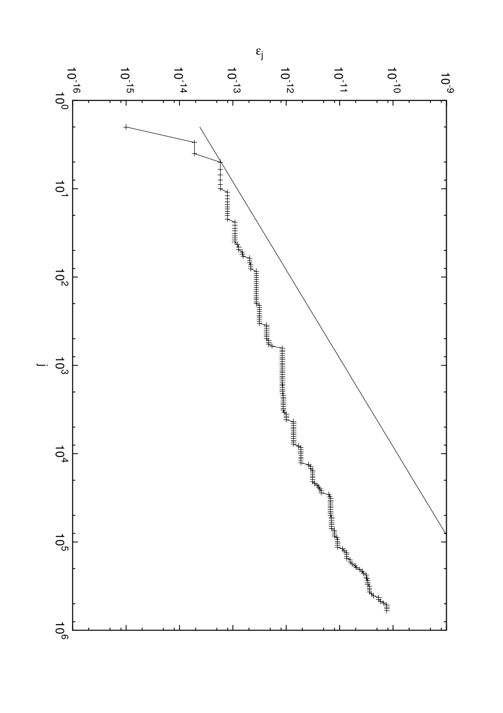
In figure 1 we draw the initial parts of the sequences $\{a_{j}\}_{j=1}^{\infty}$, $\{b_{j}\}_{j=1}^{\infty}$ for a point in the isospectral torus of the set $E^{4}$ generated by the IFS of example 1. Our technique allows for large–scale computations: in figure 2 an estimate of the infinity distance between the numerically computed elements and the true ones, i.e. $\epsilon_{j}=\max\{|b_{l}-\bar{b}_{l}|,l\leq j\}$ is plotted versus $j$. We observe a less than linear growth of the error that permits to obtain extremely accurate values even for matrix sizes in the order of hundreds of thousands.

In the previous section we have shown how to compute numerically the entries of Jacobi matrices in the isospectral torus of a finite number of intervals. It must be remarked that the same objects can also be expressed in terms of theta functions [7, 8], but this procedure seems to be numerically hard even for a small number of intervals. To the contrary, the approach adopted herein is capable of dealing satisfactorily with as many as $2^{18}$ intervals with moderate computer resources [51]. Before proceeding further with numerical techniques, we need an analytic result:

This result is the basis of our numerical approach to the isospectral torus. For instance, Figure 3 displays the function $\Psi(\alpha_{1},\alpha_{2})$ in a case composed of three intervals, i.e. two fundamental frequencies, a case that permits a graphical rendering in three dimensions. How to parameterize conveniently this function is the topic of our further development.

Let us from now on focus on the sequence of the outdiagonal matrix Jacobi matrix elements $\{b_{j}\}_{j=1}^{\infty}$, that is more significant mathematically than the sister $\{a_{j}\}_{j=0}^{\infty}$. All results will nonetheless apply also to this latter. Let us expand the analytic function $\Psi$ in Fourier series. Indicating by $\alpha$ the vector of arguments $\alpha_{1},\ldots,\alpha_{N-1}$, a $N-1$ dimensional real vector, and by $k$ a $N-1$ dimensional integer vector, we can write

The set of indices ${\cal K}$ is to be chosen so to reflect the reality of the function $\Psi$. Using this representation in eq. (18), one trivially finds that

However simple, the above equation reflects a significant, well known fact:

In equation (20), one observes the frequencies $\omega_{\mathbf{k}}:=2\pi\mathbf{k}\cdot\omega$ and the phases $\psi_{\mathbf{k}}:=2\pi\mathbf{k}\cdot\psi$. Recall that the function $\Psi$ does not depend on the specific matrix in the isospectral torus. Therefore, we discover that

The coefficient $C(\omega)$ of an almost periodic sequence $\{b_{j}\}_{j\in\mathbf{N}}$ is defined formally as the limit

We can therefore restate our approach to the isospectral torus associated with the set $E^{n}$ as follows:

To be rendered effective, this corollary needs a refined Fourier analysis of the sequence $\{b_{j}\}_{j\in\mathbf{N}}$. This can be achieved in three steps.

• $\bullet$

  We compute the frequencies $\omega_{\mathbf{k}}$. For this, we solve the set of equations (12) and we compute the fundamental frequencies $\omega^{n}_{i}$, following [49, 51].

• $\bullet$

  Using this information, we consider the numerical problem of computing the coefficients $C(\omega_{\bf k})$ in a more effective way than by the definition (21) that is theoretically significant but numerically ineffective. A technique to this aim is described in Appendix, when the set of indices ${\cal K}$ is replaced by a finite set.

• $\bullet$

  Finally, we organize the infinite set of indices as an increasing sequence of finite, nested sets.

The first two steps above being described in Appendix and in the references, let us concentrate on the third. A possibility in this respect is to use a metric in ${\mathbf{Z}}^{N-1}$, that includes ${\cal K}$, so to define

where $B_{L}$ is the ball of radius $L$ centered at the origin. Convergence of the Fourier sequence (19), when ${\cal K}$ is replaced by ${\cal K}_{L}$ and $L$ tends to infinity is a classical problem of harmonic analysis, see e.g. [25]. In Figure 4 we use the metric induced by the norm $\|\mathbf{k}\|=\sum_{i=1}^{N-1}|k_{i}|$, we set $L=8$ and we consider $E^{n}$, with $n=2$. In this case the support of the measure is made of four intervals: there are three fundamental frequencies $\omega^{2}_{i}$ and $\mathbf{k}$ is a three–dimensional vector. At the location of this vector in space, we display a color-coded point, in logarithmic scale, according to the amplitude $|C_{\mathbf{k}}|$.

We observe an exponential decrease of the amplitudes as $\|\mathbf{k}\|$ increases, that supports the relevance of the metric adopted. Yet, at an accurate inspection, this decrease is not uniform, but this observation leads to further discovery.

In fact, let us plot the values of $|C_{\mathbf{k}}|$ along lines from the origin directed as the coordinate axes. That is, fix all $k_{i}$ values to zero except one, and raise this latter from $1$ to $L$. We obtain fig. (5), now for $E^{3}$. The behavior observed for $n=3$ is typical, and consists of an exponential decay of amplitudes with $k_{i}$.

The decays starts off from the value of the amplitude of the principal harmonic $\omega^{n}_{i}$, that for simplicity we denote $|C^{n}_{i}|$. This harmonic is associated with the gap $G^{n}_{i}$ in the set $E^{n}$. It has been observed long ago in the theory of electronic states in solids, that an harmonic component in the potential of a tight binding Hamiltonian opens a gap in the spectrum of this latter. By perturbation theory arguments [67] it was established that the size of the gap is proportional to the amplitude of the harmonic component. We observe here the reverse behavior: proportionality is approximatively well verified, but it is the size of the gap that induces the amplitude of the principal harmonic: see fig. 6.

Remark that data points in figure 6 refer to four different orders $n$. Also notice that some points at different values of $n$ appear to be almost coincident. These observations are of relevance when considering the limit of infinite $n$, a thing that we shall do later on.

To conclude this section, we show in fig. 7 the harmonic amplitudes $C_{\mathbf{k}}$ versus $\omega_{\mathbf{k}}$ obtained by our technique for $n=3$. Remark two fundamental differences with respect to fig. 2 in [44] (or the analogous fig. 3.1 in [39]): a difference in technique—fast Fourier was there employed, limiting resolution, and a quite evident difference in symmetry. We are now in the presence of a typical spectrum (although still at a low value of $n$) of an IFS system. Also to test the reliability of the data so displayed, in the next section we want to tackle a difficult problem, that of convergence to the isospectral torus.

In this section we will study the convergence of Jacobi matrices of different measures supported on $E^{n}$ to their limit point in the isospectral torus. We will consider the following situation:

We denote by $\{a_{j}(\mu_{n})\}_{j\in\mathbf{N}}$, $\{b_{j}(\mu_{n})\}_{j\in\mathbf{N}}$ the sequences of Jacobi matrix elements of $\mu_{n}$. In this respect, the following theorem is notable

A comment is in order. The above theorem has been proven in [57] in a much more general setting than the one presented here. On the other hand, a strengthening of this result is possible for special classes of measures. Aptekarev [8] considered absolutely continuous measures on $E^{n}$ with densities on each interval $E^{n}_{i}$ of the kind $\rho(s)=w(s)(s-a_{i})^{\alpha_{i}}(b_{i}-s)^{\beta_{i}}$, being $\alpha_{i},\beta_{i}>-1$ and $w(s)$ locally analytical and non-negative. He proved that distance from the asymptotic limit provided by eq. (18) is asymptotically $O(1/j)$. Suetin [64], by requiring that $\rho(s)=w(s)/\sqrt{|Y(s)|}$ with a strictly positive, holomorphic $w$, proves that convergence is $O(\delta^{n})$, with a suitable constant $\delta<1$. We will now study numerically both cases.

To define measures satisfying Aptekarev or Suetin conditions, we make recourse once more to the IFS construction. Let us associate to each map $\phi_{j}$ in eq. (4) a positive weight $\pi_{j}$, $\sum_{j=1}^{M}\pi_{j}=1$ and let us define the operator $T$ acting on continuous functions on $\mathbf{R}$ given by $Tf=\sum_{j}\pi_{j}f\circ\phi_{j}$. Let $T^{*}$ be the dual operator of $T$, acting in the space of regular Borel probability measures. Then, the following theorem is standard

The devil’s staircase/Cantor measure considered in the Introduction is precisely of this kind. Observe that Theorem 6 applies to any initial measure $\mu_{0}$. We therefore make two choices. In case a) we use the normalized Lebesgue measure on $E^{0}$. In case b) $\mu_{0}$ is the (suitably rescaled) orthogonality measure of Chebyshev polynomials of second kind. It then easily follows that

Let us now apply a numerical technique for the stable computation of the Jacobi matrices $J_{\mu_{n}}$, that applies to both cases a) and b) just discussed. This technique has been introduced in ref. [46] and is radically different from the one described in [51] and in Sect. 4 of this work. On the force of the above theorems, these matrices converge to a point in the isospectral torus. This raises a challenging numerical problem.

We propose the following solution of this problem. In view of the harmonic analysis presented in Sect. 6 and of Lemma 2, we can reduce the previous problem to the determination of the shifts $\psi_{\mathbf{k}}$, for $\mathbf{k}\in{\cal K}_{L}$. It is then possible from these latter to reconstruct the precise isospectral matrix, since amplitudes and frequencies are universal in the isospectral torus and can be determined in advance. We denote by $\theta_{n}$ and $J_{\theta_{n}}$ measure and matrix in the isospectral torus that correspond to $\mu_{n}$.

Again, let us consider for simplicity the single sequence $\{b_{j}(\mu_{n})\}_{j\in\mathbf{N}}$. The associated set of phases $\psi_{\mathbf{k}}$ can be computed combining Fourier analysis with a suitable extrapolation procedure outlined in the second part of the Appendix. Let us comment here on the results that can be obtained in this way.

We start by examining case a). Fig. 8 exhibits convergence of $b_{j}(\mu_{n})$ to the corresponding matrix element $b_{j}(\theta_{n})$ of the measure $\theta_{n}$ in the isospectral torus of $E^{n}$, obtained as described above. Convergence is slow enough to permit us to appreciate visually how the two sequences are getting close.

To quantify convergence, we compute the difference $|b_{j}(\mu_{n})-b_{j}(\theta_{n})|$ and we plot it in double logarithmic scale in fig. 9. We observe that the decay of this difference is bounded from above by $A_{n}/j$, in accordance with [8]. At large values of $j$ this decay stops and difference between $b_{j}(\mu_{n})$ and $b_{j}(\theta_{n})$ oscillates at a low value due to the combination of two effects: on the one hand, computations are performed with a finite set of frequencies ${\cal K}_{L}$. When $n$ increases the cardinality of ${\cal K}_{L}$ increases as $L^{n}$, so that we are forced to reduce $L$ in order to keep the number of frequencies within acceptable limits (see Appendix). On the other hand, our Fourier analysis is performed on finite Jacobi matrices whose length is fixed, albeit large (typically, 800,000). Therefore, amplitudes and phases of $\omega^{n}_{\mathbf{k}}$ are determined less precisely when $n$ grows.

Next, let us consider case b). Figure 10 is the analogue of fig. 9, but it now compares cases a) and b) at the fixed value of $n=2$. The exponential decay of the latter is immediately appreciated.

Plotting the same data on a larger interval, and resorting to logarithmic scale, shows the $O(1/j)$ bound on the decay: see fig. 11. The exponential convergence of case b) appears even more dramatically here. The same comments on precision of the computation described above also apply in this case.

We can now conclude this section noting that the data presented confirm the validity of our approach in determining numerically the isospectral torus for finite collections of intervals. We can therefore move to the Cantor set case.

A recent paper by Krüger and Simon [39] discusses in the usual illuminating way various issues related to the definition(s) of an isospectral “torus” associated with measures supported on Cantor sets. Our approach to this problem is the following: in accordance with definition 1 we would like to define this object as

It is clear that the above definition can be extended beyond the realm of I.F.S. with a finite number of maps. Yet, we have been intentionally conservative, postponing generalizations. In fact, we believe that these hypotheses should be enough to assure weak convergence of the following procedure. Write the gaps in $E^{n}$ as:

where $H^{n}$ is the set of “new” gaps created at level $n$. $H^{n}$ is iteratively constructed as

starting from $H^{1}=(\beta^{1}_{1},\alpha^{1}_{2})\bigcup\ldots\bigcup(\beta^{1}_{M-1},\alpha^{1}_{M})$. The countable set of gaps $G^{\infty}$ in the I.F.S. Cantor set is then written as

In so doing, we can order the countable set of gaps of the Cantor set as they appear with $n$ in eq. (24), and for each $H^{n}$ in ascending order on the real line. This also imply an ordering of the infinite set of points $\{\xi_{i}\}_{i\in\mathbf{N}}$ (one in each gap) and of the Riemann surface indices $\{\sigma_{i}\}_{i\in\mathbf{N}}$.

Let us now consider such a double sequence $\{\xi_{i},\sigma_{i}\}_{i\in\mathbf{N}}$, that defines a sequence of measures $\{\theta_{n}\}_{i\in\mathbf{N}}$. If this sequence converges weakly, then the Jacobi matrix elements $a_{j}(\theta_{n})$ and $b_{j}(\theta_{n})$ also converge. As mentioned, we conjecture that IFS hyperbolicity should warrant this convergence.

Our technique permits to test this conjecture numerically. As a matter of fact, convergence seems to hold at a geometrical rate—as it might be expected, because of the hyperbolicity hypothesis. In fig. 12 we plot the absolute value of the difference $b_{j}(\theta_{n})-b_{j}(\theta_{n-1})$, versus both $n$ and $j$. On the surface defined by these values, we also plot the line $N(\varepsilon,n)$ indicating that for $j\leq N(\varepsilon,n)$ the difference between $b_{j}(\theta_{n})$ and its infinite limit is less than $\varepsilon$. This quantity is significant, because it indicates that, at precision $\varepsilon$, the truncated isospectral Jacobi matrix of rank $N(\varepsilon,n)$ is insensitive to the torus variables $\{\xi_{i},\sigma_{i}\}_{i>Q}$, with $Q=M^{n}$. As a consequence of geometric convergence, for any $\varepsilon$, $N(\varepsilon,n)$ grows asymptotically in an exponential way with $n$.

The same geometric convergence is observed in the harmonic analysis of these Jacobi matrices. This holds for both frequencies and amplitudes. For example, in Table 1 we report the fundamental frequency corresponding to the second gap in our ordering, and its amplitude. This geometrical convergence might be the key by which to resolve the conjecture mentioned in the introduction, at least numerically. We now turn to this last point in this paper.

As mentioned, the numerical techniques presented in this paper aim at providing hints to the resolution of the conjecture on the almost periodicity of hyperbolic IFS Jacobi matrices. We want to report here preliminary results in this direction. These results are not resolutive in a sense or another, but clarify the setting of the problem.

For sake of definiteness, let $\mu_{\infty}$ be the balanced measure of such an IFS, $J_{\mu}$ its Jacobi matrix, and $\{b_{j}(\mu)\}_{j\in\mathbf{N}}$ the sequence of its out-diagonal entries. Let also $\mu_{n}$ be the sequence of its IFS approximations, constructed starting from the Chebyshev measure of second kind, and $\theta_{n}$ the corresponding measures in the finite dimensional isospectral torus.

We have seen that as $j$ grows, $b_{j}(\theta_{n})$ and $b_{j}(\mu_{n})$ approach each other exponentially fast. It is now important to gauge the slope of this exponential. In figure 13 we plot the cases $n=1$ to $n=4$ for the example considered in this paper. The fitting exponential lines have form $c_{n}e^{-d_{n}j}$. They have been computed as a log-linear least squares fit, and appear to be approximately intersecting at $n\sim 1$. The important feature is then the decay coefficient $d_{n}$. In table 2 we report these values. It appears that, as $n$ grows, $d_{n}$ tends to zero. As a matter of fact, the sequence of $d_{n}$ values can be itself extremely well approximated by an exponential decay: $d_{n}\sim e^{-\delta n}$ with $\delta\simeq 0.644$.

Let us now fix a positive threshold $\varepsilon$. Extrapolating the data so far obtained, we can predict that for $j>J(\varepsilon,n)=\log(1/\varepsilon)e^{\delta n}$ the distance between $b_{j}(\theta_{n})$ and $b_{j}(\mu_{n})$ is less than $\varepsilon$.

Let us now consider the distance between $b_{j}(\mu_{n})$ and $b_{j}(\mu_{\infty})$. At difference with the previous, this distance can be bound by a fixed value $\varepsilon$ when $j$ is smaller than a value $N(\varepsilon,n)$. We therefore define $N(\varepsilon,n):=\max\{l\mbox{ s.t. }|b_{j}(\mu_{n})-b_{j}(\mu_{\infty})|\leq\varepsilon,0<j\leq l\}$. It was originally found in [46] that $N(\varepsilon,n)$ increases exponentially with $n$. Notice that the same dependence has been observed in Sect. 8 and fig. 12, but we are now in a completely different setting, because one of the terms, $\mu_{\infty}$, is the I.F.S. singular continuous measure that is the object of the debated conjecture. Suppose that it happens that for $\varepsilon$ sufficiently small, $N(\varepsilon,n)\sim e^{\kappa n}$. Then, if the inequality $\kappa>\delta$ holds, by choosing larger and larger values of $n$, the Jacobi matrix elements $b_{j}(\mu_{\infty})$ can be uniformly approximated by $b_{j}(\theta_{n})$ in the asymptotically long, asymptotically remote segments $j\in(e^{\delta n},e^{\kappa n})$.

Our original technique [43] of computing the Jacobi matrix associated with $\mu_{\infty}$ can be now put to work, in combination with that in [46], to compute the function $|b_{j}(\mu_{n})-b_{j}(\mu_{\infty})|$, that is plotted logarithmic scale in fig. 14. At the basis, the experimental curves $j(n)=N(\varepsilon,n)$ for various values of $\varepsilon$ are plotted, as well as $k(n)=e^{\delta n}$, with $\delta$ given by the extrapolation of the data in table 2. Even if the figure spans over various orders $n$ and up to Jacobi matrices of size in the hundreds of thousands, a clear-cut evidence in favor of the inequality $\kappa>\delta$, or its violation, cannot be obtained: the displayed data seem to be very close to the hedge between the two behaviors.

The harmonic problem required in this paper differs from the usual in that the frequencies present in the signal are known, being determined by eq. (20). Therefore, we act as follows. First, we multiply the “signal” $b_{j}$ by a window function $w_{j}$. For this, we choose the Dolph–Chebyshev window, well described in the classical paper [32]. Define the windowed discrete Fourier transform

Due to the property of the filter, the above is a finite summation. Next, we take into account the fact that the frequencies $\omega_{\mathbf{k}}$ are known. Since we restrict ${\mathbf{k}}$ to ${\cal K}_{L}$, this set is finite, and we can list frequencies in ascending order. Evaluating the windowed Fourier transform at any of these frequencies we find that

where $D_{\mathbf{k}^{\prime}}$ is a complex coefficient that encodes both $C_{\mathbf{k}^{\prime}}$ and $\psi_{\mathbf{k}^{\prime}}$. Actually, we work with two separate equations for real and imaginary part: this has several numerical advantages.

$W({\mathbf{k}},{\mathbf{k}^{\prime}})$ is a kernel that can be exactly computed, so that eq. (26) is a linear system for the unknowns $D_{\mathbf{k}^{\prime}}$. Taken at face value, this equation is discouraging, for the cardinality of the set ${\cal K}_{L}$ makes it untractable numerically. Yet, the Dolph-Chebyshev filter is such that $W$ is a function of the difference $\omega_{\mathbf{k}}-\omega_{\mathbf{k}^{\prime}}$, and this function can be made arbitrarily small outside of an interval centered at zero [32]. Therefore, in our numerical computations, by arranging frequencies in increasing order, $W({\mathbf{k}},{\mathbf{k}^{\prime}})$ becomes a banded matrix, and the system (26) can be swiftly solved. It is just the case to remark that this procedure yields results of a precision unattainable by the mere usage of the fast Fourier transform, that was applied to this problem in [44, 39].

Finally, a remark on the problem of extracting the phases $\psi_{\mathbf{k}}$ when examining the sequence $b_{j}(\mu_{n})$. In this case, the finite size window $w_{j}$ is shifted along the sequence, by a finite lag $l$. A sequence of lags $l_{m}$, $m=1,\ldots,M$ is performed, and the corresponding amplitudes and phases extracted. A fitting/extrapolation procedure is then performed that yields the asymptotic values $C_{\mathbf{k}}$ and $\psi_{\mathbf{k}}$. The former are then compared with those obtained by the isospectral torus to assess the validity of the procedure, while the latter yield the desired, unknown phases.

References

- [1] F. Aaron, D. Bessis, J.D. Fournier, G. Mantica, and G.A. Mezincescu, Distribution of Roots of Random Real Generalized Polynomials, J. Stat. Phys., 86 (1997) 675–705.
- [2] N.I. Akhiezer, The Classical Moment Problem, Hafner, New York, NY. (1965).
- [3] N. I. Akhieser, General theory of the P. L. Tchebycheff polynomials. Translated from the 1945 Russian original by B. Bojanov and G. Nikolov, East J. Approx. 12, 211–259 (2006).
- [4] N. I. Akhieser, Orthogonal polynomials on several intervals, Dokl. Akad. Nauk SSSR 134 9–12 (1960) (Russian); translated as Soviet Math. Dokl. 1 989–992 (1960)
- [5] V.V. Andrievskii, Constructive function theory on sets of the complex plane through potential theory and geometric function theory, Surveys in Approximation Theory, 2 1-52 (2006)
- [6] V.V. Andrievskii, On the Green function for a complement of a finite number of real intervals, Constr. Approx. 20 565–583 (2004).
- [7] A.I. Aptekarev, Asymptotic properties of polynomials orthogonal on a system of contours, and periodic motion of Toda lattices, Math. USSR Sb. 53 (1986) 233–260.
- [8] A.I. Aptekarev, Matrix Riemann–Hilbert analysis for the case of higher genus – asymptotics of polynomials orthogonal on a system of intervals, Keldysh Institute preprints 28 (2008) 233–260.
- [9] G.A. Baker, D. Bessis, P. Moussa, A family of almost periodic Schrödinger operators, Phys. A 124 61–77 (1984).
- [10] M. F. Barnsley, Fractals Everywhere, Academic Press, New York, NY (1988).
- [11] M. F. Barnsley and S. G. Demko, Iterated function systems and the global construction of fractals, Proc. R. Soc. London A 399 (1985) 243–275.
- [12] M. F. Barnsley, J. S. Geronimo and A. N. Harrington, Almost periodic Jacobi matrices associated with Julia sets for polynomials, Comm. Math. Phys. 99 303–317 (1985).
- [13] J. Bellissard, D. Bessis, and P. Moussa, Chaotic states of almost–periodic Schrödinger operators, Phys. Rev. Lett. 49 701–704 (1982).
- [14] J. Bellissard, J. Geronimo, A. Volberg, and P. Yuditski, If they are limit periodic?, arXiv:math/0401391 Published in Proc. Complex analysis and dynamical systems–dedicated to L. Zalcman (2003).
- [15] J. Bellissard, R. Lima, D. Testard, Almost periodic Schrödinger operators, in Mathematics + Physics 1, 1–64, World Sci. Publishing, Singapore, (1985).
- [16] D. Bessis, M.L. Mehta, P. Moussa, Orthogonal polynomials on a family of Cantor sets and the problem of iterations of quadratic mappings, Lett. Math. Phys. 6 123–140 (1982).
- [17] H. Brolin, Invariant sets under iterations of rational functions, Ark. Mat. 6 103-144 (1965).
- [18] J. S. Christiansen, B. Simon, M. Zinchenko, Finite gap Jacobi matrices, I. The isospectral torus, Constr. Approx. 32, 1–65 (2010).
- [19] J. S. Christiansen, B. Simon, M. Zinchenko, Finite gap Jacobi matrices, II. The Szegö class, Constr. Approx. 33, 365–403 (2011).
- [20] J. S. Christiansen, B. Simon, M. Zinchenko, Finite gap Jacobi matrices, III. Beyond the Szegö class, Constr. Approx. 35 259–272 (2012).
- [21] J. S. Christiansen, B. Simon, M. Zinchenko, Finite gap Jacobi matrices: A review, Proceedings of Symposia in Pure Mathematics 87 87–103 (2013).
- [22] J. S. Christiansen, Szegö’s theorem on Parreau-Widom sets, Adv. Math. 229 1180–1204 (2012).
- [23] H.L. Cycon, R.G. Froese, W. Kirsch, B. Simon, Schrödinger operators with application to quantum mechanics and global geometry, Springer-Verlag, Berlin (1987).
- [24] F. Delyon and B. Souillard, The rotation number for finite difference operators and its properties, Comm. Math. Phys. 89, 415–426 (1983).
- [25] C. L. Fefferman, Pointwise convergence of Fourier series, Ann. of Math. 98, 551–571 (1973).
- [26] H.-J. Fischer, Recurrence Coefficients of Orthogonal Polynomials with Respect to Some Self-Similar Singular Distributions, Z. Anal. Anwendungen 14, 141–155 (1995).
- [27] J.D. Fournier, G. Mantica, A. Mezincescu and D. Bessis, Universal Statistical Behavior of the Complex Zeros of Wiener Transfer Functions, Europhys. Lett. 22 (1993) 325–331.
- [28] W. Gautschi, Orthogonal polynomials: computation and approximation. Numerical Mathematics and Scientific Computation. Oxford Science Publications. Oxford University Press, New York, (2004)
- [29] J. S. Geronimo, W. Van Assche, Orthogonal polynomials with asymptotically periodic recurrence coefficients, J. Approx. Theory 46, 251–283 (1986).
- [30] J. S. Geronimo, W. Van Assche, Orthogonal polynomials on several intervals via a polynomial mapping, Trans. Amer. Math. Soc. 308, 559–581 (1988).
- [31] Ya. L. Geronimus, On certain asymptotic properties of polynomials. (Russian) Mat. Sbornik N. S. 23 77–88 (1948).
- [32] F. J. Harris, On the use of windows for harmonic analysis with the discrete Fourier transform, Proc. IEEE 66, 51–83 (1978).
- [33] S. M. Heilman, P. Owrutsky, and R. S. Strichartz, Orthogonal Polynomials with Respect to Self-Similar Measures, Experiment. Math. 20, (2011) 238–259.
- [34] J. Hutchinson, Fractals and self–similarity, Indiana J. Math. 30, (1981) 713–747.
- [35] P. Janardhan, D. Rosenblum and R. S. Strichartz, Numerical experiments in Fourier asymptotics of Cantor measures and wavelets, Experiment. Math. 1, 249–273 (1992).
- [36] R. A. Johnson, A review of recent work on almost periodic differential and difference operators, Acta Appl. Math. 1, 241–261 (1983).
- [37] R. A. Johnson, Cantor spectrum for the quasi-periodic Schrödinger equation, J. Differential Equations 91, 88–110 (1991).
- [38] G. Julia, Mémoire sur l’iteration des fonctions rationelles, J. Math. Ser. 7 (Paris) 4, 47–245 (1918).
- [39] H. Krüger and B. Simon, Cantor polynomials and some related classes of OPRL, J. Approx. Theory 191, 71–93 (2015).
- [40] Y. Last, Exotic spectra: a review of Barry Simon’s central contributions, in Spectral theory and mathematical physics: a Festschrift in honor of Barry Simon’s 60th birthday, Proc. Sympos. Pure Math. 76, 697–712 (2007), Amer. Math. Soc., Providence, RI.
- [41] A. Magnus, Recurrence coefficients for orthogonal polynomials on connected and nonconnected sets, in Padé approximation and its applications (Proc. Conf., Univ. Antwerp, Antwerp, 1979), Lecture Notes in Math. 765, 150–171, Springer, Berlin, (1979).
- [42] A. Magnus, Padé approximation to functions with branch points, Lecture notes 1998-1999, http://perso.uclouvain.be/alphonse.magnus/num3/m3xxx98.ps
- [43] G. Mantica, A Stieltjes Technique for Computing Jacobi Matrices Associated With Singular Measures, Constr. Appr. 12, (1996) 509–530.
- [44] G. Mantica, Quantum intermittency in almost periodic systems derived from their spectral properties, Physica D 103, (1997) 576–589.
- [45] G. Mantica, Generalized Bessel Functions: Theoretical Relevance, and Computational Techniques, in Self-Similar Systems and Orthogonal Polynomials: the Legacy of of Ya.L. Geronimus V.B. Priezzhev and V.P. Spiridonov Eds. 306-315 (1999).
- [46] G. Mantica, On Computing Jacobi Matrices associated with Recurrent and Möbius Iterated Functions Systems, J. Comp. and Appl. Math. 115 419-431 (2000).
- [47] G. Mantica, Wave propagation in almost-periodic structures, Physica D 109, (1997) 113–127.
- [48] G. Mantica, Fourier-Bessel functions of singular continuous measures and their many asymptotics, Electron. Trans. Numer. Anal. (Electronic) 25, (2006) 409–430.
- [49] G. Mantica, Computing the equilibrium measure of a system of intervals converging to a Cantor set, DRNA (Electronic) 6, 51–61 (2013).
- [50] G. Mantica, Direct and inverse computation of Jacobi matrices of infinite IFS, Numerische Math. 125, (2013) 705–731.
- [51] G. Mantica, Orthogonal polynomials of equilibrium measures supported on Cantor sets, arXiv:1311.4819 [math.NA], (2013). Submitted to J. Comp. Appl. Math.
- [52] P. A. P. Moran, Additive functions of intervals and Hausdorff measure, Proc. Camb. Phil. Soc. 42, (1946) 15–23.
- [53] J. Nuttall and S. R. Singh, Orthogonal polynomials and Padé approximants associated with a system of arcs, J. Approx. Theory 21, (1977) 1-42.
- [54] F. Peherstorfer, On Bernstein-Szegö orthogonal polynomials on several intervals, SIAM J. Math. Anal. 21, (1990) 461-482.
- [55] F. Peherstorfer, Orthogonal and extremal polynomials on several intervals, J. Comput. Appl. Math. 48 (1993) 187–205.
- [56] F. Peherstorfer, Zeros of polynomials orthogonal on several intervals, Int. Math. Res. Not. 7 (2003) 361–385.
- [57] F. Peherstorfer, P. Yuditskii, Asymptotic behavior of polynomials orthonormal on a homogeneous set, J. Anal. Math. 89 113–154 (2003).
- [58] L. Perotti, T. Regimbau, D. Vrinceanu, and D. Bessis, Identification of gravitational-wave bursts in high noise using Padé filters, Phys. Rev. D, 90 (2014) 124047.
- [59] T. Ransford, Potential theory in the complex plane, Cambridge University Press, Cambridge (1995).
- [60] E. B. Saff, Logarithmic potential theory with applications to approximation theory, Surveys in Approx. Theory 5 (2010) 165–200.
- [61] W. B. Jones, O. Njastad, E. B. Saff, Szegö polynomials associated with Wiener-Levinson filters, J. Comp. App. Math. 32 (1990) 387–406.
- [62] K. Pan, E. B. Saff, Asymptotics for zeros of Szegö polynomials associated with trigonometric polynomial signals, J. Approx. Theory 71 (1992) 239–251.
- [63] H. Stahl, V. Totik, General Orthogonal Polynomials, Cambridge University Press, Cambridge (2010).
- [64] S. P. Suetin, Trace formulae for a class of Jacobi Operators, Math. Sbornik 198 (2007) 857–885.
- [65] A. Süto, Singular continuous spectrum on a Cantor set of zero Lebesgue measure for the Fibonacci Hamiltonian, J. Statist. Phys. 56 525–531 (1989).
- [66] V. Totik, Metric properties of harmonic measures, Mem. Am. Math. Soc. 184 n. 867, (2006).
- [67] P. Turchi, F. Ducastelle, and G. Treglia, Band gaps and asymptotic behaviour of continued fraction coefficients, Journal of Physics C: Solid State Physics 15 2891 (1982).
- [68] W. Van Assche, Asymptotics for orthogonal polynomials and three-term recurrences, in Orthogonal Polynomials; Theory and Practice, NATO-ASI series C 294, 435–462 (1990).
- [69] H. Widom, Extremal polynomials associated with a system of curves in the complex plane, Adv. in Math. 3 (1969) 127–232.