On Graduated Optimization for Stochastic
Non-Convex Problems

Elad Hazan Note: Princeton University; ehazan@cs.princeton.edu. Kfir Y. Levy Note: Technion; kfiryl@tx.technion.ac.il. Shai Shalev-Shwartz Note: The Hebrew University; shais@cs.huji.ac.il.

May 2014

Abstract

The graduated optimization approach, also known as the continuation method, is a popular heuristic to solving non-convex problems that has received renewed interest over the last decade. Despite its popularity, very little is known in terms of theoretical convergence analysis.

In this paper we describe a new first-order algorithm based on graduated optimization and analyze its performance. We characterize a parameterized family of non-convex functions for which this algorithm provably converges to a global optimum. In particular, we prove that the algorithm converges to an $\varepsilon$ -approximate solution within $O(1/\varepsilon^{2})$ gradient-based steps. We extend our algorithm and analysis to the setting of stochastic non-convex optimization with noisy gradient feedback, attaining the same convergence rate. Additionally, we discuss the setting of “zero-order optimization”, and devise a a variant of our algorithm which converges at rate of $O(d^{2}/\varepsilon^{4})$ .

1 Introduction

Non-convex optimization programs are ubiquitous in machine learning and computer vision. Of particular interest are non-convex optimization problem that arise in the training of deep neural networks Bengio (2009). Often, such problems admit a multimodal structure, and therefore, the use of convex optimization machinery may lead to a local optima.

Graduated optimization (a.k.a. continuation), Blake and Zisserman (1987), is a methodology that attempts to overcome such numerous local optima. At first, a coarse-grained version of the problem is generated by a local smoothing operation. This coarse-grained version is easier to solve. Then, the method advances in stages by gradually refining the problem versions, using the solution of the previous stage as an initial point for the optimization in the next stage.

Despite its popularity, there are still many gaps concerning both theoretical and practical aspects of graduated optimization, and in particular we are not aware of a rigorous running time analysis to find a global optimum, or even conditions in which a global optimum is reached. Nor are we familiar with graudated optimization in the stochastic setting, in which only a noisy gradient or value oracle to the objective is given. Moreover, any practical application of graduated optimization requires an efficient construction of coarse-grained versions of the original function. For some special cases this construction can be made analytically Chapelle et al. (2006); Chaudhuri and Solar-Lezama (2011) . However, in the general case, it is commonly suggested in the literature to convolve the original function with a gaussian kernel Wu (1996). Yet, this operation is prohibitively inefficient in high dimensions.

In this paper we take an algorithmic / analytic approach to graduated optimization and show the following.

•

We characterise a family of non-convex multimodal functions that allows convergence to a global optimum. This parametrized family we call $\sigma$ -nice (see Definition 4.2 ).
•

We provide a stochastic algorithm inspired by graduated optimization, that performs only gradient updates and is ensured to find an $\varepsilon$ -optimal solution of $\sigma$ -nice functions within $O(1/\sigma^{2}\varepsilon^{2})$ iterations. The algorithm doesn’t require expensive convolutions and access the smoothed version of any function using random sampling. The algorithm only requires access to the objective function through a noisy gradient oracle.
•

We extend our method to the “zero-order optimization” model (a.k.a. “bandit feedback” model), in which the objective is only accessible through a noisy value oracle. We devise a variant of our algorithm that is guaranteed to find an $\varepsilon$ -optimal solution within $O(d^{2}/\sigma^{2}\varepsilon^{4})$ iterations.

Interestingly, the next question is raised in Bengio (2009) which reviews recent developments in the field of deep learning: “Can optimization strategies based on continuation methods deliver significantly improved training of deep architectures?”

As an initial empirical study, we examine the task of training a NN (Neural Network) over the MNIST data set. Our experiments support the theoretical guarantees, demonstrating that graduated optimization according to the methodology proposed accelerates convergence in training the NN. Moreover, we show examples in which $\sigma$ -nice functions capture non-convex structure/phenomena that exists in natural data.

1.1 Related Work

Among the machine vision community, the idea of graduated optimization was known since the 80’s. The term “Graduated Non-Convexity” (GNC) was coined by Blake and Zisserman (1987), who were the first to establish this idea explicitly. Similar attitudes in the machine vision literature appeared later in Yuille (1989); Yuille et al. (1990), and Terzopoulos (1988).

Concepts of the same nature appeared in the optimization literature Wu (1996), and in the field of numerical analysis Allgower and Georg (1990).

Over the last two decades, this concept was successfully applied to numerous problems in computer vision; among are: image deblurring Boccuto et al. (2002) , image restoration Nikolova et al. (2010), and optical flow Brox and Malik (2011). The method was also adopted by the machine learning community, demonstrating effective performance in tasks such as semi-supervised learning Chapelle et al. (2006), graph matching Zaslavskiy et al. (2009), and ranking Chapelle and Wu (2010). In Bengio (2009), it is suggested to consider some developments in deep belief architectures Hinton et al. (2006); Erhan et al. (2009) as a kind of continuation. These approaches, in the spirit of the continuation method, offer no guarantees on the quality of the obtained solution, and are tailored to specific applications.

A comprehensive survey of the graduated optimization literature can be found in Mobahi and Fisher III (2015a).

A recent work Mobahi and Fisher III (2015b) advances our theoretical understanding, by analyzing a continuation algorithm in the general setting. Yet, they offer no way to perform the smoothing efficiently, nor a way to optimize the smoothed versions; but rather assume that these are possible. Moreover, their guarantee is limited to a fixed precision that depends on the objective function and does not approach zero. In contrast, our approach can generate arbitrarily precise solutions.

2 Setting

We discuss an optimization of a non-convex loss function $f:\mathcal{K}\mapsto{\mathbb{R}}$ , where $\mathcal{K}\subseteq{\mathbb{R}}^{d}$ is a convex set. We assume that optimization lasts for $T$ rounds; On each round $t=1,\ldots,T$ , we may query a point $\mathbf{x}_{t}\in\mathcal{K}$ , and receive a feedback. After the last round, we choose $\bar{\mathbf{x}}_{T}\in\mathcal{K}$ , and our performance measure is the excess loss, defined as:

f(\bar{\mathbf{x}}_{T})-\min_{\mathbf{x}\in\mathcal{K}}f(\mathbf{x})

In Section 4.2 we characterize a family of non-convex multimodal functions we call $\sigma$ -nice. Given such a $\sigma$ -nice loss $f$ , we are interested in algorithms that with a high probability ensure a $\varepsilon$ -excess loss within $\text{poly}(1/\varepsilon)$ rounds.

We consider two kinds of feedback:

1.

Noisy Gradient feedback: Upon querying $\mathbf{x}_{t}$ we receive $\nabla f(\mathbf{x}_{t})+\xi_{t}$ , where $\{\xi_{\tau}\}_{\tau=1}^{T}$ are independent zero mean and bounded r.v.’s.
2.

Noisy Value feedback (Bandit feedback): Upon querying $\mathbf{x}_{t}$ we receive $f(\mathbf{x}_{t})+\xi_{t}$ , where $\{\xi_{\tau}\}_{\tau=1}^{T}$ are independent zero mean and bounded r.v.’s.

3 Preliminaries and Notation

Notation:

During this paper we use $\mathbb{B},\mathbb{S}$ to denote the unit Euclidean ball/sphere in ${\mathbb{R}}^{d}$ , and also $\mathbb{B}_{r}(\mathbf{x}),\mathbb{S}_{r}(\mathbf{x})$ as the Euclidean $r$ -ball/sphere in ${\mathbb{R}}^{d}$ centered at $\mathbf{x}$ . For a set $A\subset{\mathbb{R}}^{d}$ , $\mathbf{u}\sim A$ denotes a random variable distributed uniformly over $A$ .

3.1 Strong-Convexity

Recall the definition of strongly-convex functions:

Definition 3.1.

(Strong Convexity) We say that a function $F:{\mathbb{R}}^{n}\to{\mathbb{R}}$ is $\sigma$ -strongly convex over the set $\mathcal{K}$ if for all $\mathbf{x},\mathbf{y}\in\mathcal{K}$ it holds that,

\displaystyle F(\mathbf{y})\geq F(\mathbf{x})+\nabla F(\mathbf{x})^{\top}(\mathbf{y}-\mathbf{x})+\frac{\sigma}{2}\|\mathbf{x}-\mathbf{y}\|^{2}

Let $F$ be a $\sigma$ -strongly convex over convex set $\mathcal{K}$ , and let $\mathbf{x}^{*}$ be a point in $\mathcal{K}$ where $F$ is minimized, then the following inequality is satisfied:

\displaystyle\frac{\sigma}{2}\|\mathbf{x}-\mathbf{x}^{*}\|^{2}\leq F(\mathbf{x})-F(\mathbf{x}^{*})

(1)

This is immediate by the definition of strong convexity combined with $\nabla F(\mathbf{x}^{*})^{\top}(\mathbf{x}-\mathbf{x}^{*})\geq 0,\;\forall\mathbf{x}\in\mathcal{K}$ .

4 Smoothing and $\sigma$ -Nice functions

Constructing finer and finer approximations to the original objective function is at the heart of the continuation approach. In Section 4.1 we define the smoothed versions that we will employ. Next, in Section 4.1.1 we describe an efficient way to implicitly access the smoothed versions, which will enable us to perform optimization. Finally, in Section 4.2 we define a class of non-convex multimodal functions we denote as $\sigma$ -nice. As we will see in Section 7, these functions are rich enough to capture non-convex structure that exists in natural data. Additionally, these functions lend themselves to an efficient optimization, and we can ensure a convergence to $\varepsilon$ -solution within $\text{poly}(1/\varepsilon)$ iterations, as described in Sections 5,6.

4.1 Smoothing

Smoothing by local averaging is formally defined next.

Definition 4.1.

Given an $L$ -Lipschitz function $f:{\mathbb{R}}^{d}\mapsto{\mathbb{R}}$ define it’s $\delta$ -smooth version to be

{\hat{f}}_{\delta}(\mathbf{x})=\mbox{\bf E}_{\mathbf{u}\sim\mathbb{B}}[f(\mathbf{x}+\delta\mathbf{u})].

The next lemma bounds the bias between ${\hat{f}}_{\delta}$ and $f$ .

Lemma 4.1.

Let $\hat{f}_{\delta}$ be the $\delta$ -smoothed version of $f$ , then,

\forall\mathbf{x}\in{\mathbb{R}}^{d}:|\hat{f}_{\delta}(\mathbf{x})-f(\mathbf{x})|\leq\delta L

Proof of Lemma 4.1.

	$\displaystyle\|\hat{f}_{\delta}(\mathbf{x})-f(\mathbf{x})\|$	$\displaystyle=\|\mbox{\bf E}_{u\sim\mathbb{B}}\left[f(\mathbf{x}+\delta\mathbf{u})\right]-f(\mathbf{x})\|$
		$\displaystyle\leq\mbox{\bf E}_{\mathbf{u}\sim\mathbb{B}}\left[\|f(\mathbf{x}+\delta\mathbf{u})-f(\mathbf{x})\|\right]$
		$\displaystyle\leq\mbox{\bf E}_{\mathbf{u}\sim\mathbb{B}}\left[L\\|\delta\mathbf{u}\\|\right]$
		$\displaystyle\leq L\delta$

in the first inequality we used Jensen’s inequality, and in the last inequality we used $\|\mathbf{u}\|\leq 1$ , since $\mathbf{u}\in\mathbb{B}$ . ∎

4.1.1 Implicit Smoothing using Sampling

A direct way to optimize a smoothed version is by direct calculation of its gradients, nevertheless this calculation might be very costly in high dimensions. A much more efficient approach is to produce an unbiased estimate for the gradients of the smoothed version by sampling the function gradients/values. These estimates could then be used by a stochastic optimization algorithms such as SGD (Stochastic Gradient Descent). This sampling approach is outlined in Figures 1,2.

Oracle 1: $\text{SGO}_{G}$

Input: $\mathbf{x}\in{\mathbb{R}}^{d}$ , smoothing parameter $\delta$

Return: $\nabla f(\mathbf{x}+\delta\mathbf{u})$ , where $\mathbf{u}\sim\mathbb{B}$

Figure 1: Smoothed gradient oracle given gradient feedback.

Oracle 2: $\text{SGO}_{V}$

Input: $\mathbf{x}\in{\mathbb{R}}^{d}$ , smoothing parameter $\delta$

Return: $\frac{d}{\delta}f(\mathbf{x}+\delta\mathbf{v})\mathbf{v}$ , where $\mathbf{v}\sim\mathbb{S}$

Figure 2: Smoothed gradient oracle given value feedback.

The following two Lemmas state that the resulting estimates are unbiased and bounded:

Lemma 4.2.

Let $\mathbf{x}\in{\mathbb{R}}^{d}$ , $\delta\geq 0$ , and suppose that $f$ is $L$ -Lipschitz, then the output of $\text{SGO}_{G}$ (Figure 1) is bounded by $L$ and is an unbiased estimate for $\nabla{\hat{f}}_{\delta}(\mathbf{x})$ .

Proof.

$\text{SGO}_{G}$ outputs $\nabla f(\mathbf{x}+\delta\mathbf{u})$ for some $\mathbf{u}\in\mathbb{B}$ , so the first part is immediate by the Lipschitzness of $f$ . Now, by definition, ${\hat{f}}_{\delta}(\mathbf{x})=\mbox{\bf E}_{\mathbf{u}\sim\mathbb{B}}[f(\mathbf{x}+{\delta}\mathbf{u})]$ , deriving both sides we get the second part of the Lemma. ∎

Lemma 4.3.

Let $\mathbf{x}\in\mathcal{K}\subseteq{\mathbb{R}}^{d}$ , $\delta\geq 0$ , and suppose that $\max_{\mathbf{x}}|f(\mathbf{x})|\leq C$ , then the output of $\text{SGO}_{V}$ (Figure 2) is bounded by $\frac{dC}{\delta}$ and is an unbiased estimate for $\nabla{\hat{f}}_{\delta}(\mathbf{x})$ .

Proof.

$\text{SGO}_{V}$ outputs $\frac{d}{\delta}f(\mathbf{x}+\delta\mathbf{v})\mathbf{v}$ for some $\mathbf{v}\in\mathbb{S}$ , since $f$ is $C$ -Bounded over $\mathcal{K}$ the first part of the lemma is immediate. In order to prove the second part, we can use Stokes theorem to show that if $\mathbf{v}\sim\mathbb{S}$ , then:

\forall\mathbf{x}\in{\mathbb{R}}^{d}\ .\ \mbox{\bf E}_{\mathbf{v}\sim\mathbb{S}}[f(\mathbf{x}+\delta\mathbf{v})\mathbf{v}]=\frac{\delta}{d}\nabla\hat{f}_{\delta}(\mathbf{x})

(2)

A proof of Equation (2) is found in Flaxman et al. (2005).

∎

Note that the oracles depicted in Figures 1, 2 may require sampling function values outside $\mathcal{K}$ , (specifically in $\mathcal{K}+\delta\mathbb{B}$ ). We assume that this is possible, and that the bounds over the function gradients/values inside $\mathcal{K}$ , also apply in $\mathcal{K}+\delta\mathbb{B}$ .

Extensions to the noisy feedback settings:

Note that for ease of notation, the oracles that appear in Figures 1, 2, assume we can access exact gradients/values of $f$ . Given that we may only access noisy and bounded gradient/value estimates of $f$ (Sec. 2), we could use these instead of the exact ones that appear in Figures 1,2, and still produce unbiased and bounded gradient estimates for the smoothed versions of $f$ as shown in Lemmas 4.2,4.3.

Particularly, in the case we may only access noisy gradients of $f$ , then $\text{SGO}_{G}$ (Figure 1) will return $\nabla f(\mathbf{x}+\delta\mathbf{u})+\xi$ instead of $\nabla f(\mathbf{x}+\delta\mathbf{u})$ , where $\xi$ is a noise term. Since we assume zero bias and bounded noise this implies that $\nabla f(\mathbf{x}+\delta\mathbf{u})+\xi$ is an unbiased estimate of $\nabla{\hat{f}}_{\delta}(\mathbf{x})$ , bounded by $L+K$ where $K$ is the bound on the noise and $L$ is the Lipschitz constant of $f$ . We can show the same for $\text{SGO}_{V}$ (Figure 2), given a noisy value feedback.

4.2 $\sigma$ -Nice Functions

Following is our main definition

Definition 4.2.

A function $f:\mathcal{K}\mapsto{\mathbb{R}}$ is said to be $\sigma$ -nice if the following two conditions hold:

1.

Centering property: For every $\delta>0$ , and every $\mathbf{x}^{*}_{\delta}\in\argmin_{\mathbf{x}\in\mathcal{K}}{\hat{f}}_{\delta}(\mathbf{x})$ , there exists $\mathbf{x}^{*}_{\delta/2}\in\arg\min_{x\in\mathcal{K}}{\hat{f}}_{\delta/2}(\mathbf{x})$ , such that:

$\|\mathbf{x}^{*}_{\delta}-\mathbf{x}^{*}_{\delta/2}\|\leq\frac{\delta}{2}$
2.

Local strong convexity of the smoothed function: For every $\delta>0$ let $r_{\delta}=3\delta$ , and denote $\mathbf{x}^{*}_{\delta}=\argmin_{\mathbf{x}\in\mathcal{K}}{\hat{f}}_{\delta}(\mathbf{x})$ , then over $B_{r_{\delta}}(\mathbf{x}^{*}_{\delta})$ , the function ${\hat{f}}_{\delta}(\mathbf{x})$ is $\sigma$ -strongly-convex.

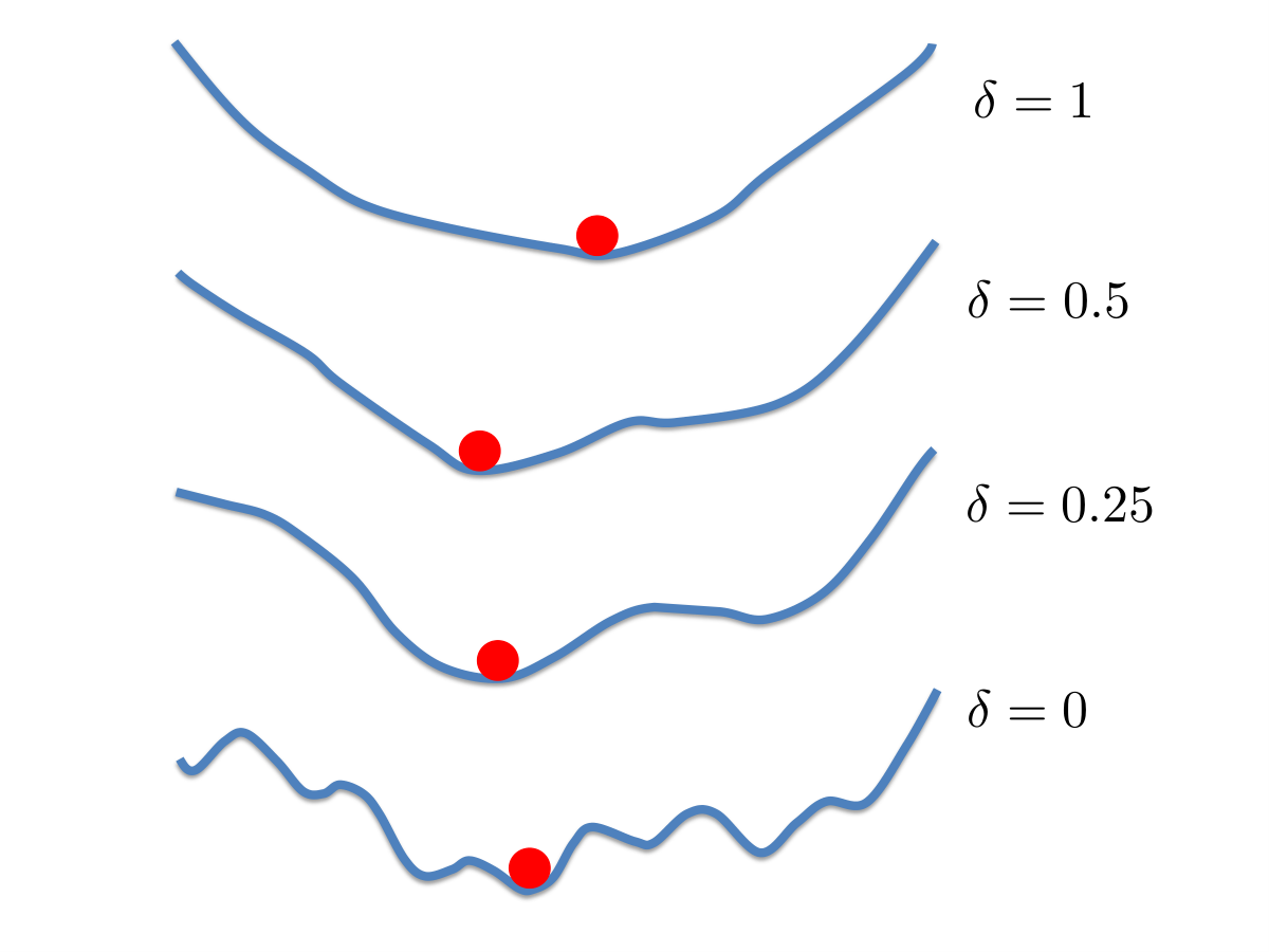
Hence, $\sigma$ -nice is a combination of two properties. Both together imply that optimizing the smoothed version on a scale $\delta$ is a good start for optimizing a finer version on a scale of $\delta/2$ , which is sufficient for a scheme based on graduated optimization to work as we show next. In Section 7 we show that $\sigma$ -nice functions arise naturally in data. An illustration of $\sigma$ -nice function in $1$ -dimension appears in Figure 3.

Refer to caption — Figure 3: A $1$ -dim $\sigma$ -nice function ( $\delta=0$ ), and its smoothed versions.

5 Graduated Optimization with a Gradient Oracle

In this section we assume that we can access a noisy gradient oracle for $f$ .

Thus, given $\mathbf{x}\in{\mathbb{R}}^{d},\delta\geq 0$ we can use $\text{SGO}_{G}$ (Figure 1) to obtain an unbiased and bounded estimate for $\nabla{\hat{f}}_{\delta}(\mathbf{x})$ , as ensured by Lemma 4.2. Note that for ease of notation $\text{SGO}_{G}$ (Figure 1) is listed using an exact gradient oracle for $f$ . As described at the end of Section 4.1.1, this could be replaced with a noisy gradient oracle for $f$ , and Lemma 4.2, will still hold.

Following is our main Theorem:

Theorem 5.1.

Let $\varepsilon\in(0,1)$ and $p\in(0,1/e)$ , also let $\mathcal{K}$ be a convex set, and $f$ be an $L$ -Lipschitz $\sigma$ -nice function. Suppose that we apply Algorithm 1, then after $\tilde{O}(1/\sigma^{2}\varepsilon^{2})$ rounds Algorithm 1 outputs a point $\bar{\mathbf{x}}_{M+1}$ which is $\varepsilon$ optimal with a probability greater than $1-p$ .

Algorithm 1

\text{GradOpt}_{G}

Input: target error

\varepsilon

, maximal failure probability

p

, decision set

\mathcal{K}

Choose

\bar{\mathbf{x}}_{1}\in\mathcal{K}

uniformly at random.

Set

\delta_{1}=\textrm{diam}(\mathcal{K})/2

\tilde{p}=p/M

, and

M=\log_{2}\frac{1}{\alpha_{0}\varepsilon}

where

\alpha_{0}=\min\{\frac{1}{2L\textrm{diam}(\mathcal{K})},\frac{2\sqrt{2}}{\sqrt{\sigma}\textrm{diam}(\mathcal{K})}\}

for

m=1

M

// Perform SGD over

{\hat{f}}_{\delta_{m}}

Set

\varepsilon_{m}:=\sigma\delta_{m}^{2}/32

, and

T_{F}=\frac{12480L^{2}}{\sigma\varepsilon_{m}}\log\big(\frac{2}{\tilde{p}}+2\log\frac{12480L^{2}}{\sigma\varepsilon_{m}}\big)

Set shrinked decision set,

\mathcal{K}_{m}:=\mathcal{K}\cap B(\bar{x}_{m},1.5\delta_{m})

Set gradient oracle for

{\hat{f}}_{\delta_{m}}

\text{GradOracle}(\cdot)=\text{SGO}_{G}(\cdot,\delta_{m})

Update:

\bar{\mathbf{x}}_{m+1}\leftarrow\text{Suffix-SGD}(T_{F},\mathcal{K}_{m},\bar{\mathbf{x}}_{m},\text{GradOracle})

\delta_{m+1}=\delta_{m}/2

end for

Return:

\bar{\mathbf{x}}_{M+1}

Algorithm 2 Suffix-SGD

Input: total time

T_{F}

, decision set

\mathcal{K}

, initial point

\mathbf{x}_{1}\in\mathcal{K}

, gradient oracle

\text{GradOracle}(\cdot)

for

t=1

T_{F}

Set

\eta_{t}=1/\sigma t

Query the gradient oracle at

\mathbf{x}_{t}

g_{t}\leftarrow\text{GradOracle}(\mathbf{x}_{t})

Update:

\mathbf{x}_{t+1}\leftarrow\Pi_{\mathcal{K}}(\mathbf{x}_{t}-\eta_{t}g_{t})

end for

Return:

\bar{\mathbf{x}}_{T_{F}}:=\frac{2}{T_{F}}\big(\mathbf{x}_{T_{F}/2+1}+\ldots+\mathbf{x}_{T_{F}}\big)

Algorithm 1 is divided into epochs, at epoch $m$ it uses $\text{SGO}_{G}$ to obtain unbiased estimates for the gradients of ${\hat{f}}_{\delta_{m}}$ which are then employed by Suffix-SGD (Algorithm 2), to optimize this smoothed version. This optimization over ${\hat{f}}_{\delta_{m}}$ is performed until we are ensured to reach a point close enough to $\mathbf{x}^{*}_{m+1}:=\argmin_{\mathbf{x}\in\mathcal{K}}{\hat{f}}_{\delta_{m+1}}(\mathbf{x})$ , i.e., the minimum of ${\hat{f}}_{\delta_{m+1}}$ . Also note that at epoch $m$ the optimization over ${\hat{f}}_{\delta_{m}}$ is initialized at $\bar{\mathbf{x}}_{m}$ which is the point reached at the previous epoch.

Suffix-SGD (Algorithm 2), is a stochastic optimization algorithm for strongly convex functions. Its guarantees are presented in Section 5.1.

5.1 Analysis

Let us first discuss Suffix-SGD (Algorithm 2). This algorithm performs projected gradient descent using the gradients received from $\text{GradOracle}(\cdot)$ . The projection operator $\Pi_{\mathcal{K}}$ , is defined $\forall\mathbf{y}\in{\mathbb{R}}^{d}$ as

\Pi_{\mathcal{K}}(\mathbf{y}):=\argmin_{\mathbf{x}\in\mathcal{K}}\|\mathbf{x}-\mathbf{y}\|~.

Now consider a $\sigma$ -strongly convex function $F:\mathcal{K}\to{\mathbb{R}}$ , and suppose that we have an oracle, $\text{GradOracle}(\cdot)$ , that upon querying a point $\mathbf{x}\in\mathcal{K}$ returns an unbiased and bounded gradient estimate, $g$ , i.e., $\mbox{\bf E}[g]=\nabla F(x)$ , and $\|g\|\leq G$ . Note the following result from Rakhlin et al. (2011) regarding stochastic optimization of $\sigma$ -strongly-convex functions, given such an oracle:

Theorem 5.2.

Let $p\in(0,1/e)$ , and $F$ be a $\sigma$ -strongly convex function. Suppose that $\text{GradOracle}(\cdot)$ produces G-bounded, and unbiased estimates of $\nabla F$ . Then after no more than $T_{F}$ rounds, the final point $\bar{\mathbf{x}}_{T_{F}}$ returned by Suffix-SGD (Algorithm 2 ) ensures that with a probability $\geq 1-p$ , we have:

F(\bar{\mathbf{x}}_{T_{F}})-\min_{\mathbf{x}\in\mathcal{K}}F(\mathbf{x})\leq\frac{6240\log\big(2\log(T_{F})/p\big)G^{2}}{\sigma T_{F}}

Corollary 5.1.

The latter means that for $T_{F}\geq\frac{12480G^{2}}{\sigma\varepsilon}\log\big(2/p+2\log(12480G^{2}/\sigma\varepsilon)\big)$ we will have an excess loss smaller than $\varepsilon$ .

Notice that at each epoch $m$ of $\text{GradOpt}_{G}$ , it initiates Suffix-SGD with a gradient oracle $\text{SGO}_{G}(\cdot,\delta_{m})$ . According to Lemma 4.2, $\text{SGO}_{G}(\cdot,\delta_{m})$ produces an unbiased and $L$ -bounded estimates of ${\hat{f}}_{\delta_{m}}$ , thus in the analysis of each epoch we can use Theorem 5.2 for ${\hat{f}}_{\delta_{m}}$ , taking $G=L$ .

Following is our key Lemma:

Lemma 5.1.

Consider $M$ , $\mathcal{K}_{m}$ and $\bar{\mathbf{x}}_{m+1}$ as defined in Algorithm 1. Also denote by $\mathbf{x}^{*}_{m}$ the minimizer of ${\hat{f}}_{\delta_{m}}$ in $\mathcal{K}$ . Then the following holds for all $1\leq m\leq M$ w.p. $\geq 1-p$ :

1.

The smoothed version ${\hat{f}}_{\delta_{m}}$ is $\sigma$ -strongly convex over $\mathcal{K}_{m}$ , and $\mathbf{x}_{m}^{*}\in\mathcal{K}_{m}$ .
2.

Also, ${\hat{f}}_{\delta_{m}}(\bar{\mathbf{x}}_{m+1})-{\hat{f}}_{\delta_{m}}(\mathbf{x}_{m}^{*})\leq\sigma\delta_{m+1}^{2}/8$

Proof.

We will prove by induction, let us prove it holds for $m=1$ . Note that $\delta_{1}=\textrm{diam}(\mathcal{K})/2$ , therefore $\mathcal{K}_{1}=\mathcal{K}$ , and also $\mathbf{x}_{1}^{*}\in\mathcal{K}_{1}$ . Also recall that $\sigma$ -niceness of $f$ implies that ${\hat{f}}_{\delta_{1}}$ is $\sigma$ -strongly convex in $\mathcal{K}$ , thus by Corollary 5.1, after less than $T_{F}=\tilde{\mathcal{O}}(\frac{12480L^{2}}{\sigma(\sigma\delta_{1}^{2}/32)})$ optimization steps of Suffix-SGD with a probability greater than $1-p/M$ , we will have:

{\hat{f}}_{\delta_{1}}(\bar{\mathbf{x}}_{2})-{\hat{f}}_{\delta_{1}}(\mathbf{x}_{1}^{*})\leq\sigma\delta_{1}^{2}/32=\sigma\delta_{2}^{2}/8

which establishes the case of $m=1$ . Now assume that lemma holds for $m>1$ . By this assumption, ${\hat{f}}_{\delta_{m}}(\bar{\mathbf{x}}_{m+1})-{\hat{f}}_{\delta_{m}}(\mathbf{x}_{m}^{*})\leq\sigma\delta_{m+1}^{2}/8$ , ${\hat{f}}_{\delta_{m}}$ is $\sigma$ -strongly convex in $\mathcal{K}_{m}$ , and also $\mathbf{x}_{m}^{*}\in\mathcal{K}_{m}$ . Hence, we can use Equation (1) to get:

\|\bar{\mathbf{x}}_{m+1}-\mathbf{x}_{m}^{*}\|\leq\sqrt{\frac{2}{\sigma}}\sqrt{{\hat{f}}_{\delta_{m}}(\bar{\mathbf{x}}_{m+1})-{\hat{f}}_{\delta_{m}}(\mathbf{x}_{m}^{*})}=\frac{\delta_{m+1}}{2}

Combining the latter with the centering property of $\sigma$ -niceness yields:

	$\displaystyle\\|\bar{\mathbf{x}}_{m+1}-\mathbf{x}_{m+1}^{*}\\|$	$\displaystyle\leq\\|\bar{\mathbf{x}}_{m+1}-\mathbf{x}_{m}^{}\\|+\\|\mathbf{x}_{m}^{}-\mathbf{x}_{m+1}^{*}\\|$
		$\displaystyle\leq 1.5\delta_{m+1}$

and it follows that,

\mathbf{x}_{m+1}^{*}\in B(\bar{\mathbf{x}}_{m+1},1.5\delta_{m+1})\subset B({\mathbf{x}}_{m+1}^{*},3\delta_{m+1})

Recalling that $\mathcal{K}_{m+1}:=B(\bar{\mathbf{x}}_{m+1},1.5\delta_{m+1})$ , and the local strong convexity property of $f$ (which is $\sigma$ -nice), then the induction step for first part of the lemma holds. Now, by Corollary 5.1, after less than $T_{F}=\tilde{\mathcal{O}}(\frac{12480L^{2}}{\sigma(\sigma\delta_{m+1}^{2}/32)})$ optimization steps of Suffix-SGD over ${\hat{f}}_{\delta_{m+1}}$ , we will have:

{\hat{f}}_{\delta_{m+1}}(\bar{\mathbf{x}}_{m+2})-{\hat{f}}_{\delta_{m+1}}(\mathbf{x}_{m+1}^{*})\leq\sigma\delta_{m+2}^{2}/8

which establishes the induction step for the second part of the lemma.

An analysis of fail probability: since we have $M$ epochs in total and at each epoch the fail probability is smaller than $p/M$ , then the total fail probability of our algorithm is smaller than $p$ . ∎

We are now ready to prove Theorem 5.1:

proof of Theorem 5.1.

Algorithm 1 terminates after $M=\log_{2}\frac{1}{\alpha_{0}\varepsilon}$ epochs meaning, $\delta_{M}=\textrm{diam}(\mathcal{K})\alpha_{0}\varepsilon/2$ . According to Lemma 5.1 the following holds w.p. $\geq 1-p$ , for every $\mathbf{x}\in\mathcal{K}$ ,

	$\displaystyle{\hat{f}}_{\delta_{M}}(\bar{\mathbf{x}}_{M+1})-{\hat{f}}_{\delta_{M}}(\mathbf{x})$	$\displaystyle\leq\sigma\delta_{M+1}^{2}/8$
		$\displaystyle=\left(\frac{\sqrt{\sigma}\textrm{diam}(\mathcal{K})\alpha_{0}\varepsilon}{8\sqrt{2}}\right)^{2}$

Due to Lemma 4.1, ${\hat{f}}_{\delta_{M}}$ is $L\delta_{M}$ biased from $f$ , thus for every $\mathbf{x}\in\mathcal{K}$ ,

	$\displaystyle f(\bar{\mathbf{x}}_{M+1})-f(\mathbf{x})$	$\displaystyle\leq L\textrm{diam}(\mathcal{K})\alpha_{0}\varepsilon+\left(\frac{\sqrt{\sigma}\textrm{diam}(\mathcal{K})\alpha_{0}\varepsilon}{8\sqrt{2}}\right)^{2}$
		$\displaystyle\leq\varepsilon$

we used $\alpha_{0}=\min\{\frac{1}{2L\textrm{diam}(\mathcal{K})},\frac{2\sqrt{2}}{\sqrt{\sigma}\textrm{diam}(\mathcal{K})}\}$ , and $\varepsilon<1$ .

Let $T_{\text{total}}$ , be the total number of queries made by Algorithm 1, then we have:

	$\displaystyle T_{\text{total}}$	$\displaystyle\leq\sum_{m=1}^{M}\frac{12480L^{2}}{\sigma\varepsilon_{m}}\log\Gamma$
		$\displaystyle\leq\sum_{m=1}^{M}\frac{12480L^{2}}{\sigma(\sigma\delta_{m}^{2}/32)}\log\Gamma$
		$\displaystyle\leq\frac{4\cdot 10^{5}L^{2}\log\Gamma}{\sigma^{2}}\sum_{i=1}^{M}\frac{4^{i-1}}{\delta_{1}^{2}}$
		$\displaystyle\leq\frac{14\cdot 10^{4}L^{2}\log\Gamma}{\sigma^{2}}\frac{4^{M}}{\delta_{1}^{2}}$
		$\displaystyle\leq\frac{14\cdot 10^{4}L^{2}\log\Gamma}{\sigma^{2}}\max\{{16L^{2}},{\sigma}/{2}\}\frac{1}{\varepsilon^{2}}$

here we used the notation:

	$\displaystyle\Gamma$	$\displaystyle:=\frac{2M}{p}+2\log(12480L^{2}/\sigma\varepsilon_{M})$
		$\displaystyle\leq\frac{2M}{p}+2\log(4\cdot 10^{5}L^{2}\max\{{16L^{2}},\frac{\sigma}{2}\}/\sigma^{2}\varepsilon^{2})$

∎

6 Graduated Optimization with a Value Oracle

In this section we assume that we can access a noisy value oracle for $f$ .

Thus, given $\mathbf{x}\in{\mathbb{R}}^{d},\delta\geq 0$ we can use $\text{SGO}_{V}$ (Figure 2) as an oracle that outputs an unbiased and bounded estimates for $\nabla{\hat{f}}_{\delta}(\mathbf{x})$ , as ensured by Lemma 4.3. Note that for ease of notation $\text{SGO}_{V}$ (Figure 2) is listed using an exact value oracle for $f$ . As described at the end of Section 4.1.1, this could be replaced with a noisy value oracle for $f$ , and Lemma 4.3, will still hold.

Following is our main Theorem:

Theorem 6.1.

Let $\varepsilon>0$ and $p\in(0,1/e)$ , also let $\mathcal{K}$ be a convex set, and $f$ be an $L$ -Lipschitz $\sigma$ -nice function. Assume also that $\max_{\mathbf{x}}|f(\mathbf{x})|\leq C$ . Suppose that we apply Algorithm 3, then after after $\tilde{O}(d^{2}/\sigma^{2}\varepsilon^{4})$ rounds Algorithm 3 outputs a point $\bar{\mathbf{x}}_{M+1}$ which is $\varepsilon$ optimal with a probability greater than $1-p$ .

Algorithm 3

\text{GradOpt}_{V}

Input: target error

\varepsilon

, maximal failure probability

p

, decision set

\mathcal{K}

Choose

\bar{\mathbf{x}}_{1}\in\mathcal{K}

uniformly at random.

Set

\delta_{1}=\textrm{diam}(\mathcal{K})/2

\tilde{p}=p/M

, and

M=\log_{2}\frac{1}{\alpha_{0}\varepsilon}

where

\alpha_{0}=\min\{\frac{1}{2L\textrm{diam}(\mathcal{K})},\frac{2\sqrt{2}}{\sqrt{\sigma}\textrm{diam}(\mathcal{K})}\}

for

m=1

M

// Perform SGD over

{\hat{f}}_{\delta_{m}}

Set

\varepsilon_{m}:=\sigma\delta_{m}^{2}/32

, and

T_{F}=\frac{12480}{\sigma\varepsilon_{m}}\frac{d^{2}C^{2}}{\delta_{m}^{2}}\log\big(\frac{2}{\tilde{p}}+2\log\frac{12480d^{2}C^{2}}{\sigma\varepsilon_{m}\delta_{m}^{2}}\big)

Set shrinked decision set,

\mathcal{K}_{m}:=\mathcal{K}\cap B(\bar{x}_{m},1.5\delta_{m})

Set gradient oracle for

{\hat{f}}_{\delta_{m}}

\text{GradOracle}(\cdot)=\text{SGO}_{V}(\cdot,\delta_{m})

Update:

\bar{\mathbf{x}}_{m+1}\leftarrow\text{Suffix-SGD}(T_{F},\mathcal{K}_{m},\bar{\mathbf{x}}_{m},\text{GradOracle})

\delta_{m+1}=\delta_{m}/2

end for

Return:

\bar{\mathbf{x}}_{M+1}

6.1 Analysis

Notice that at each epoch $m$ of $\text{GradOpt}_{V}$ , it initiates Suffix-SGD with a gradient oracle $\text{SGO}_{V}(\cdot,\delta_{m})$ . According to Lemma 4.3, $\text{SGO}_{V}(\cdot,\delta_{m})$ produces an unbiased and ${dC}/{\delta_{m}}$ -bounded estimates for the gradients of ${\hat{f}}_{\delta_{m}}$ , thus in the analysis of each epoch we can use Corollary 5.1 for ${\hat{f}}_{\delta_{m}}$ , taking $G={dC}/{\delta_{m}}$ .

Following is our key Lemma:

Lemma 6.1.

Consider $M$ , $\mathcal{K}_{m}$ and $\bar{\mathbf{x}}_{m+1}$ as defined in Algorithm 3. Also denote by $\mathbf{x}^{*}_{m}$ the minimizer of ${\hat{f}}_{\delta_{m}}$ in $\mathcal{K}$ . Then the following holds for all $1\leq m\leq M$ w.p. $\geq 1-p$ :

1.

The smoothed version ${\hat{f}}_{\delta_{m}}$ is $\sigma$ -strongly convex over $\mathcal{K}_{m}$ , and $\mathbf{x}_{m}^{*}\in\mathcal{K}_{m}$ .
2.

Also, ${\hat{f}}_{\delta_{m}}(\bar{\mathbf{x}}_{m+1})-{\hat{f}}_{\delta_{m}}(\mathbf{x}_{m}^{*})\leq\sigma\delta_{m+1}^{2}/8$

The proof of Lemma 6.1 is similar to the proof of Lemma 5.1 given in Section 5.1, we therefore omit the details.

We are now ready to prove Theorem 6.1:

proof of Theorem 6.1.

Let $\bar{\mathbf{x}}_{M+1}$ be the output of Algorithm 3. Similarly to the proof of Theorem 5.1, we can show that for every $\mathbf{x}\in\mathcal{K}$ :

\displaystyle f(\bar{\mathbf{x}}_{M+1})-f(\mathbf{x})\leq\varepsilon

Let $T_{\text{total}}$ , be the total number of queries made by Algorithm 3, then we have:

	$\displaystyle T_{\text{total}}$	$\displaystyle\leq\sum_{m=1}^{M}\frac{12480d^{2}C^{2}}{\sigma\varepsilon_{m}\delta_{m}^{2}}\log\Gamma$
		$\displaystyle\leq\sum_{m=1}^{M}\frac{12480d^{2}C^{2}}{\sigma(\sigma\delta_{m}^{2}/32)\delta_{m}^{2}}\log\Gamma$
		$\displaystyle\leq\frac{4\cdot 10^{5}d^{2}C^{2}\log\Gamma}{\sigma^{2}}\sum_{i=1}^{M}\frac{8^{i-1}}{\delta_{1}^{4}}$
		$\displaystyle\leq\frac{6\cdot 10^{4}d^{2}C^{2}\log\Gamma}{\sigma^{2}}\frac{8^{M}}{\delta_{1}^{4}}$
		$\displaystyle\leq\frac{6\cdot 10^{4}d^{2}C^{2}\log\Gamma}{\sigma^{2}}\max\{{256L^{4}},{\sigma^{2}}/{4}\}\frac{1}{\varepsilon^{4}}$

here we used the notation:

	$\displaystyle\Gamma$	$\displaystyle:=\frac{2M}{p}+2\log(12480d^{2}C^{2}/\sigma\varepsilon_{M}\delta_{M}^{2})$
		$\displaystyle\leq\frac{2M}{p}+2\log(4\cdot 10^{5}d^{2}C^{2}\max\{{256L^{4}},\frac{{\sigma^{2}}}{4}\}/\sigma^{2}\varepsilon^{4})$

∎

7 Experiments

In the last two decades, performing complex learning tasks using Neural-Network (NN) architectures has become an active and promising line of research. Since learning NN architectures essentially requires to solve a hard non-convex program, we have decided to focus our empirical study on this type of tasks. As a test case, we train a NN with a single hidden layer of $30$ units over the MNIST data set. We adopt the experimental setup of Dauphin et al. (2014) and train over a down-scaled version of the data, i.e., the original $28\times 28$ images of MNIST were down-sampled to the size of $10\times 10$ . We use a ReLU activation function, and minimize the square loss.

Figure 4: The objective near a stall point. Left:

\delta=0

. Middle:

\delta=3

. Right:

\delta=7

7.1 Smoothing the NN

First, we were interested in exploring the non-convex structure of the above NN learning task, and check whether our definition of $\sigma$ -nice complies with this structure. We started by running MSGD (Minibatch Stochastic Gradient Descent) on the problem, while using a batch size of $100$ , and a step size rule of the form $\eta_{t}=\eta_{0}(1+\gamma t)^{-3/4}$ , where $\eta_{0}=0.01,\;\gamma=10^{-4}$ . This choice of step size rule was the most effective among a grid of rules that we examined. We have found out that MSGD frequently “stalls” in areas with a relatively high loss, here we relate to points at the end of such run as stall-points.

In order to learn about the non-convex nature of the problem, we examined the objective values along two directions around stall-points. The first direction was the gradient at the stall point, and the second direction was the line connecting the stall-point to $\mathbf{x}^{*}$ , where $\mathbf{x}^{*}$ is the best weights configuration of the NN that we were able to find. A drawing depicting typical results appears on the left side of Figure 4. The stall-point appears in red, and $\mathbf{x}^{*}$ in green; also the axis marked as $X$ is the gradient direction, and one marked $Y$ is the direction between stall-point and $\mathbf{x}^{*}$ . Note that the stall-point is inside a narrow “valley”, which prevents MSGD from “seeing” $\mathbf{x}^{*}$ , and so it seems that MSGD slowly progresses downstream. Interestingly, the objective around $x^{*}$ seems strongly-convex in the direction of the stall point.

On the middle of Figure 4, we present the $\delta=3$ smoothed version of the same objective that appears on the left side of Figure 4. We can see that the “valley” has not vanished, but the gradient of the smoothed version leads us slightly towards $\mathbf{x}^{*}$ and out of the original “valley”. On the right side of Figure 4, we present the $\delta=7$ smoothed version of the objective. We can see that due to the coarse smoothing, the “valley” in which MSGD was stalled, has completely dissolved, and the gradient of this version leads us towards $\mathbf{x}^{*}$ .

7.2 Graduated Optimization of NN

Here we present experiments that demonstrate the effectiveness of $\text{GradOpt}_{G}$ (Algorithm 1) in training the NN mentioned above. First, we wanted to learn if smoothing can help us escape points where MSGD stalls. We used MSGD ( $\delta=0$ ) to train the NN, and as before we found that its progress slows down, yielding relatively high error. We then took the point that MSGD reached after $5\cdot 10^{4}$ iteration and initialized an optimization over the smoothed versions of the loss; this was done using smoothing values of $\{1,3,5,7\}$ . In Figure 5 we present the results of the above experiment.

Figure 5: Running optimization with fixed smoothing values, starting at the point where MSGD stuck after

5\cdot 10^{4}

iterations.

As seen in Figure 5, small $\delta$ ’s converge slower than large $\delta$ ’s, but produce a much better solution. Furthermore, the initial optimization progresses in leaps, for large $\delta$ ’s the leaps are sharper, and lower $\delta$ ’s demonstrate smaller leaps. We believe that these leaps are associated with the advance of the optimization from one local “valley” to another; Larger values of $\delta$ dissolve the “valleys” much easily, but converge to points with higher errors than small $\delta$ ’s, due to the increase of the bias with smoothing.

In Figure 6 we compare our complete graduated optimization algorithm, namely $\text{GradOpt}_{G}$ (Alg. 1) to MSGD. We started with an initial smoothing of $\delta=7$ , which decayed according to $\text{GradOpt}_{G}$ . Note that $\text{GradOpt}_{G}$ progresses very fast and yields a much better solution than MSGD.

Figure 6: Comparison between MSGD and

\text{GradOpt}_{G}

8 Discussion

We have described a family of non-convex functions which admit efficient optimization via the graduated optimization methodology, and gave the first rigorous analysis of a first-order algorithm in the stochastic setting.

We view it as only a first glimpse of the potential of graduated optimization to provable non-convex optimization, and amongst the interesting questions that remain we find

•

Is $\sigma$ -niceness necessary for convergence of first-order methods to a global optimum? Is there a more lenient property that better captures the power of graduated optimization?
•

Amongst the two properties of $\sigma$ -niceness, can their parameters be relaxed in terms of the ratio of smoothing to strong-convexity, or to centering?
•

Can second-order/other methods give rise to better convergence rates / faster algorithms for stochastic or offline $\sigma$ -nice non-convex optimization?

References

Allgower and Georg (1990) E. L. Allgower and K. Georg. Numerical continuation methods, volume 13. Springer-Verlag Berlin, 1990.
Bengio (2009) Y. Bengio. Learning deep architectures for ai. Foundations and trends in Machine Learning, 2(1):1–127, 2009.
Blake and Zisserman (1987) A. Blake and A. Zisserman. Visual reconstruction, volume 2. MIT press Cambridge, 1987.
Boccuto et al. (2002) A. Boccuto, M. Discepoli, I. Gerace, R. Pandolfi, and P. Pucci. A gnc algorithm for deblurring images with interacting discontinuities. Proc. VI SIMAI, pages 296–310, 2002.
Brox and Malik (2011) T. Brox and J. Malik. Large displacement optical flow: descriptor matching in variational motion estimation. IEEE Transactions on Pattern Analysis and Machine Intelligence, 33(3):500–513, 2011.
Chapelle and Wu (2010) O. Chapelle and M. Wu. Gradient descent optimization of smoothed information retrieval metrics. Information retrieval, 13(3):216–235, 2010.
Chapelle et al. (2006) O. Chapelle, M. Chi, and A. Zien. A continuation method for semi-supervised svms. In Proceedings of the 23rd international conference on Machine learning, pages 185–192. ACM, 2006.
Chaudhuri and Solar-Lezama (2011) S. Chaudhuri and A. Solar-Lezama. Smoothing a program soundly and robustly. In Computer Aided Verification, pages 277–292. Springer, 2011.
Dauphin et al. (2014) Y. N. Dauphin, R. Pascanu, C. Gulcehre, K. Cho, S. Ganguli, and Y. Bengio. Identifying and attacking the saddle point problem in high-dimensional non-convex optimization. In Advances in Neural Information Processing Systems, pages 2933–2941, 2014.
Erhan et al. (2009) D. Erhan, P.-A. Manzagol, Y. Bengio, S. Bengio, and P. Vincent. The difficulty of training deep architectures and the effect of unsupervised pre-training. In International Conference on Artificial Intelligence and Statistics, pages 153–160, 2009.
Flaxman et al. (2005) A. Flaxman, A. T. Kalai, and H. B. McMahan. Online convex optimization in the bandit setting: gradient descent without a gradient. In SODA, pages 385–394, 2005.
Hinton et al. (2006) G. Hinton, S. Osindero, and Y.-W. Teh. A fast learning algorithm for deep belief nets. Neural computation, 18(7):1527–1554, 2006.
Mobahi and Fisher III (2015a) H. Mobahi and J. W. Fisher III. On the link between gaussian homotopy continuation and convex envelopes. In Energy Minimization Methods in Computer Vision and Pattern Recognition, pages 43–56. Springer, 2015a.
Mobahi and Fisher III (2015b) H. Mobahi and J. W. Fisher III. A theoretical analysis of optimization by gaussian continuation. 2015b.
Nikolova et al. (2010) M. Nikolova, M. K. Ng, and C.-P. Tam. Fast nonconvex nonsmooth minimization methods for image restoration and reconstruction. IEEE Transactions on Image Processing, 19(12):3073, 2010.
Rakhlin et al. (2011) A. Rakhlin, O. Shamir, and K. Sridharan. Making gradient descent optimal for strongly convex stochastic optimization. arXiv preprint arXiv:1109.5647, 2011.
Terzopoulos (1988) D. Terzopoulos. The computation of visible-surface representations. IEEE Transactions on Pattern Analysis and Machine Intelligence, 10(4):417–438, 1988.
Wu (1996) Z. Wu. The effective energy transformation scheme as a special continuation approach to global optimization with application to molecular conformation. SIAM Journal on Optimization, 6(3):748–768, 1996.
Yuille (1989) A. Yuille. Energy functions for early vision and analog networks. Biological Cybernetics, 61(2):115–123, 1989.
Yuille et al. (1990) A. L. Yuille, D. Geiger, and H. Bülthoff. Stereo integration, mean field theory and psychophysics. In Computer Vision ECCV 90, pages 71–82. Springer, 1990.
Zaslavskiy et al. (2009) M. Zaslavskiy, F. Bach, and J.-P. Vert. A path following algorithm for the graph matching problem. Pattern Analysis and Machine Intelligence, IEEE Transactions on, 31(12):2227–2242, 2009.

	$\displaystyle\|\hat{f}_{\delta}(\mathbf{x})-f(\mathbf{x})\|$	$\displaystyle=\|\mbox{\bf E}_{u\sim\mathbb{B}}\left[f(\mathbf{x}+\delta\mathbf{u})\right]-f(\mathbf{x})\|$
		$\displaystyle\leq\mbox{\bf E}_{\mathbf{u}\sim\mathbb{B}}\left[\|f(\mathbf{x}+\delta\mathbf{u})-f(\mathbf{x})\|\right]$
		$\displaystyle\leq\mbox{\bf E}_{\mathbf{u}\sim\mathbb{B}}\left[L\\|\delta\mathbf{u}\\|\right]$
		$\displaystyle\leq L\delta$

On Graduated Optimization for Stochastic Non-Convex Problems

Abstract

1 Introduction

1.1 Related Work

2 Setting

3 Preliminaries and Notation

Notation:

3.1 Strong-Convexity

Definition 3.1.

4 Smoothing and σ\sigma-Nice functions

4.1 Smoothing

Definition 4.1.

Lemma 4.1.

Proof of Lemma 4.1.

4.1.1 Implicit Smoothing using Sampling

Lemma 4.2.

Proof.

Lemma 4.3.

Proof.

Extensions to the noisy feedback settings:

4.2 σ\sigma-Nice Functions

Definition 4.2.

5 Graduated Optimization with a Gradient Oracle

Theorem 5.1.

5.1 Analysis

Theorem 5.2.

Corollary 5.1.

Lemma 5.1.

Proof.

proof of Theorem 5.1.

6 Graduated Optimization with a Value Oracle

Theorem 6.1.

6.1 Analysis

Lemma 6.1.

proof of Theorem 6.1.

7 Experiments

7.1 Smoothing the NN

7.2 Graduated Optimization of NN

8 Discussion

References

On Graduated Optimization for Stochastic
Non-Convex Problems

4 Smoothing and $\sigma$ -Nice functions

4.2 $\sigma$ -Nice Functions