\copyrightdata

978-1-nnnn-nnnn-n/yy/mm nnnnnnn.nnnnnnn

\authorinfo

Chang Yao^‡, Divyakant Agrawal^♯, Gang Chen^§, Beng Chin Ooi^‡, Sai Wu^§ ^‡National University of Singapore, ^♯University of California at Santa Barbara, ^§Zhejiang University ^‡{yaochang,ooibc}@comp.nus.edu.sg, ^♯agrawal@cs.ucsb.edu, ^§{cg,wusai}@cs.zju.edu.cn

Adaptive Logging for Distributed In-memory Databases

Conference: Submission to SoCC ’15 August, 2015, Hawaii, USA

Abstract

A new type of logs, the command log, is being employed to replace the traditional data log (e.g., ARIES log) in the in-memory databases. Instead of recording how the tuples are updated, a command log only tracks the transactions being executed, thereby effectively reducing the size of the log and improving the performance. Command logging on the other hand increases the cost of recovery, because all the transactions in the log after the last checkpoint must be completely redone in case of a failure. In this paper, we first extend the command logging technique to a distributed environment, where all the nodes can perform recovery in parallel. We then propose an adaptive logging approach by combining data logging and command logging. The percentage of data logging versus command logging becomes an optimization between the performance of transaction processing and recovery to suit different OLTP applications. Our experimental study compares the performance of our proposed adaptive logging, ARIES-style data logging and command logging on top of H-Store. The results show that adaptive logging can achieve a 10x boost for recovery and a transaction throughput that is comparable to that of command logging.

1 Introduction

Harizopoulos et al. Harizopoulos et al. [2008] show that in in-memory databases, substantial amount of time is spent in logging, latching, locking, index maintenance, and buffer management. The existing techniques in relational databases will lead to suboptimal performance for in-memory databases, because the assumption of I/O being the main bottleneck is no longer valid. For instance, in conventional databases, the most widely used logging approach is the write-ahead log (e.g., ARIES log Mohan et al. [1992a]). Write-ahead logging records the history of transactional updates to the data tuples, and we shall refer to it as the data log in this paper.

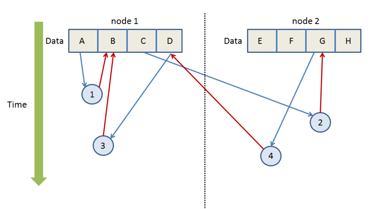
Refer to caption — Figure 1: Example of logging techniques

Consider an example shown in Figure 1. There are two nodes processing four concurrent transactions, $T_{1}$ to $T_{4}$ . All the transactions follow the same format:

f(x,y):y=2x

So $T_{1}=f(A,B)$ , indicating that $T_{1}$ reads the value of $A$ and then updates $B$ as $2A$ . Since different transactions may modify the same value, there should be a locking mechanism. Based on their timestamps, the correct serialized order of the transactions is $T_{1}$ , $T_{2}$ , $T_{3}$ and $T_{4}$ . Let $v(X)$ denote the value of parameter $X$ . The ARIES data log of the four transactions are listed as below:

Table 1: ARIES log

timestamp	transaction ID	parameter	old value	new value
100001	$T_{1}$	B	v(B)	2v(A)
100002	$T_{2}$	G	v(G)	2v(C)
100003	$T_{3}$	B	v(B)	2v(D)
100004	$T_{4}$	D	v(D)	2v(G)

ARIES log records how the data are modified by the transactions, and by using the log data, we can efficiently recover if there is a node failure. However, the recovery process of in-memory databases is sightly different from that of conventional disk-based databases. To recover, an in-memory database first loads the database snapshot recorded in the last checkpoint and then replays all the committed transactions in ARIES log. For uncommitted transactions, no roll-backs are required, since uncommitted writes will not be reflected onto disk.

ARIES log is a “heavy-weight” logging approach, as it incurs high overheads. In conventional database systems, where I/Os for processing transactions dominate the performance, the logging cost is tolerable. However, in an in-memory system, since all the transactions are processed in memory, logging cost becomes a dominant cost.

To reduce the logging overhead, a command logging approach Malviya et al. [2014] was proposed to only record the transaction information with which transaction can be fully replayed when facing a failure. In H-Store Kallman et al. [2008], each command log records the ID of the corresponding transaction and which stored procedure is applied to update the database along with input parameters. As an example, the command logging records for Figure 1 are simplified as below:

Table 2: Command log

transaction ID	timestamp	procedure pointer	parameters
1	100001	$p$	A, B
2	100002	$p$	C, G
3	100003	$p$	D, B
4	100004	$p$	G, D

As all four transactions follow the same routine, we only keep a pointer $p$ to the details of storage procedure: $f(x,y):y=2x$ . For recovery purposes, we also need to maintain the parameters for each transaction, so that the system can re-execute all the transactions from the last checkpoint when a failure happens. Compared to ARIES-style log, a command log is much more compact and hence reduces the I/O cost for materializing it onto disk. It was shown that command logging can significantly increase the throughput of transaction processing in in-memory databases Malviya et al. [2014]. However, the improvement is achieved at the expense of its recovery performance.

When there is a node failure, all the transactions have to be replayed in the command logging approach, while ARIES-style logging simply recovers the value of each column (Note that throughout the paper, we use ”attribute” to refer to a column defined in the schema and ”attribute value” to denote the value of a tuple in a specific column). For example, to fully redo $T_{1}$ , command logging needs to read the value of $A$ and update the value of $B$ , while if ARIES logging is adopted, we just set $B$ ’s value as $2v(A)$ as recorded in the log file. More importantly, command logging does not support parallel recovery in a distributed system. In the command logging Malviya et al. [2014], command logs of different nodes are merged at the master node during recovery, and to guarantee the correctness of recovery, transactions must be reprocessed in a serialized order based on their timestamps. For example, even in a network of two nodes, the transactions have to be replayed one by one due to their possible competition. For the earlier example, $T_{3}$ and $T_{4}$ cannot be concurrently processed by node 1 and 2 respectively, because both transactions need to lock the value of $D$ . For comparison, ARIES-style logging can start the recovery in node 1 and 2 concurrently and independently.

In summary, command logging reduces the I/O cost of processing transactions, but incurs a much higher cost for recovery than ARIES-style logging, especially in a distributed environment. To this end, we propose a new logging scheme which achieves a comparable performance as command logging for processing transactions, while enabling a much more efficient recovery. Our logging approach also allows the users to tune the parameters to achieve a preferable tradeoff between transaction processing and recovery.

In this paper, we first propose a distributed version of command logging. In the recovery process, before redoing the transactions, we first generate the dependency graph by scanning the log data. Transactions that read or write the same tuple will be linked together. A transaction can be reprocessed only if all its dependent transactions have been processed and committed. On the other hand, transactions that do not have dependency relationship can be concurrently processed. Based on this principle, we organize transactions into different processing groups. Transactions inside a group have dependency relationship, while transactions of different groups can be processed concurrently.

While distributed version of command logging effectively exploits the parallelism among the nodes to speed up recovery, some processing groups can be rather large, causing a few transactions to block the processing of many others. We subsequently propose an adaptive logging approach which adaptively makes use of the command logging and ARIES-style logging. More specifically, we identify the bottlenecks dynamically based on our cost model and resolve them using ARIES logging. We materialize the transactions identified as bottlenecks in ARIES log. So transactions depending on them can be recovered more efficiently.

It is indeed very challenging to classify transactions into the ones that may cause bottleneck and those that will not, because we have to make a real-time decision on either adopting command logging or ARIES logging. During transaction processing, we do not know the impending distribution of transactions. Even if the dependency graph of impending transactions is known before the processing starts, we note that the optimization problem of log creation is still an NP-hard problem. Hence, a heuristic approach is subsequently proposed to find an approximate solution based on our model. The idea is to estimate the importance of each transaction based on the access patterns of existing transactions.

Finally, we implement our two approaches, namely distributed command logging and adaptive logging, on top of H-Store Kallman et al. [2008] and compare them with ARIES logging and command logging. Our results show that adaptive logging can achieve a comparable performance for transaction processing as command logging, while it performs 10 times faster than command logging for recovery in a distributed system.

The rest of the paper is organized as follows. We present our distributed command logging approach in Section 2 and the new adaptive logging approach in Section 3. The experimental results are presented in Section 4 and we review some related work in Section 5. The paper is concluded in Section 6.

2 Distributed Command Logging

As described earlier, the command logging Malviya et al. [2014] only records the transaction ID, storage procedure and its input parameters. If some servers fail, the database can restore the last snapshot and redo all the transactions in the command log to re-establish the database state. Command logging operates at a much coarser granularity and writes much fewer bytes per transaction than ARIES-style logging.

However, the major concern of command logging is its recovery performance. In VoltDB¹¹ 1 http://voltdb.com/, command logs of different nodes are shuffled to the master node which merges them using the timestamp order. Since command logging does not record how the data are manipulated, we must redo all transactions one by one, incurring high recovery overhead. An alternative solution is to maintain multiple replicas Baker et al. [2011]; Corbett et al. [2013]; Rao et al. [2011]; Thomson et al. [2012]; Haughian [2014], so that data on the failed node can be recovered from their replicas. However, the drawback of such approach is twofold. First, keeping consistency between replicas incurs high synchronization overhead, further slowing down the transaction processing. Second, given a limited amount of memory, it is too expensive to maintain replicas in memory. Therefore, in this paper, we focus on the log-based approaches, although we also show the performance of a replication-based technique in our experimental study.

Before delving into the details of our approach, we first define the correctness of recovery in our system. Suppose the data are partitioned to $N$ cluster nodes. Let $\mathcal{T}$ be the set of transactions since the last checkpoint. For a transaction $t_{i}\in\mathcal{T}$ , if $t_{i}$ reads or writes a tuple on node $n_{x}\in N$ , $n_{x}$ becomes a participant of $t_{i}$ . Specifically, we use $f(t_{i})$ to return all those nodes involved in $t_{i}$ and we use $f^{-1}(n_{x})$ to represent all the transactions in which $n_{x}$ has participated. In a distributed system, we will assign each transaction a coordinator, typically the node that minimizes the data transfer for processing the transaction. The coordinator schedules the data accesses and monitors how its transaction is processed. Hence, we only need to create a command log entry in the coordinator Malviya et al. [2014]. We use $\theta(t_{i})$ to denote $t_{i}$ ’s coordinator. Obviously, we have $\theta(t_{i})\in f(t_{i})$ .

Given two transactions $t_{i}\in\mathcal{T}$ and $t_{j}\in\mathcal{T}$ , we define an order function $\prec$ as: $t_{i}\prec t_{j}$ , only if $t_{i}$ is committed before $t_{j}$ . When a node $n_{x}$ fails, we need to redo a set of transactions $f^{-1}(n_{x})$ . But these transactions may compete for the same tuple with other transactions. Let $s(t_{i})$ and $c(t_{i})$ denote the submission time and commit time respectively.

Definition 1

Transaction Competition
Transaction $t_{i}$ competes with transaction $t_{j}$ , if

1.

$s(t_{j})<s(t_{i})<c(t_{j})$ .
2.

$t_{i}$ and $t_{j}$ read or write the same tuple.

Note that we define the competition as a unidirectional relationship. $t_{i}$ competes with $t_{j}$ , and $t_{j}$ may compete with others which may modify the same set of tuples and commit before it. Let $\odot(t_{i})$ be the set of all the transactions that $t_{i}$ competes with. We define function $g$ for transaction set $\mathcal{T}_{j}$ as:

g(\mathcal{T}_{j})=\bigcup_{\forall t_{i}\in\mathcal{T}_{j}}\odot(t_{i})

To recover the database from $n_{x}$ ’s failure, we create an initial recovery set $\mathcal{T}^{x}_{0}=f^{-1}(n_{x})$ and set $\mathcal{T}^{x}_{i+1}=\mathcal{T}^{x}_{i}\cup g(\mathcal{T}^{x}_{i})$ . As we have a limited number of transactions, we can find a $L$ satisfying when $j\geq L$ , we have $\mathcal{T}^{x}_{j+1}=\mathcal{T}^{x}_{j}$ . This is because there are no more transactions accessing the same set of tuples since the last checkpoint. We call $\mathcal{T}^{x}_{L}$ the complete recovery set for $n_{x}$ .

Finally, we define the correctness of recovery in the distributed system as:

Definition 2

Correctness of Recovery
When node $n_{x}$ fails, we need to redo all the transactions in its complete recovery set by strictly following their commit order, e.g., if $t_{i}\prec t_{j}$ , then $t_{i}$ must be reprocessed before $t_{j}$ .

To recover from a node’s failure, we need to retrieve its complete recovery set. For this purpose, we build a dependency graph.

2.1 Dependency Graph

Dependency graph is defined as an acyclic direct graph $G=(V,E)$ , where each vertex $v_{i}$ in $V$ represents a transaction $t_{i}$ , containing the information about its timestamp ( $c(t_{i})$ and $s(t_{i})$ ) and coordinator $\theta(t_{i})$ . $v_{i}$ has an edge $e_{ij}$ to $v_{j}$ , iff

1.

$t_{i}\ in\odot(t_{j})$
2.

$\forall t_{m}\in\odot(t_{j}),c(t_{m})<c(t_{i})$

Figure 2: A running example

For a specific order of transaction processing, there is one unique dependency graph as shown in the following theorem.

Theorem 1

Given a transaction set $\mathcal{T}=\{t_{0},...,t_{k}\}$ , where $c(t_{i})<c(t_{i+1})$ , we can generate a unique dependency graph for $\mathcal{T}$ .

Proof 1

Since the vertices represent transactions, we always have the same set of vertices for the same set of transactions. We only need to prove that the edges are also unique. Based on the definition, edge $e_{ij}$ exists, only if $t_{j}$ accesses the same set of tuples that $t_{i}$ updates and no other transactions that commit after $t_{i}$ have that property. As for each transaction $t_{j}$ , there is only one such transaction $t_{i}$ . Therefore, edge $e_{ij}$ is a unique edge between $t_{i}$ and $t_{j}$ .

We use Figure 2 as a running example to illustrate the idea. In Figure 2, there are totally seven transactions since the last checkpoint, aligned based on their coordinators: node 1 and node 2. We show transaction IDs, timestamps, storage procedures and parameters in the table. Based on the definition, transaction $t_{2}$ competes with transaction $t_{1}$ , as both of them update $x_{1}$ . Transaction $t_{4}$ competes with transaction $t_{2}$ on $x_{3}$ . The complete recovery set for $t_{4}$ is $\{t_{1},t_{2},t_{4}\}$ . Note that although $t_{4}$ does not access the attribute that $t_{1}$ updates, $t_{1}$ is still in $t_{4}$ ’s recovery set because of the recursive dependency between $t_{1}$ , $t_{2}$ and $t_{4}$ . After constructing the dependency graph and generating the recovery set, we can adaptively recover the failed node. For example, to recover node 1, we do not have to reprocess transactions $t_{3}$ and $t_{5}$ .

2.2 Processing Group

In order to generate the complete recovery set efficiently, we organize transactions as processing groups. Algorithm 1 and 2 illustrate how we generate the groups from a dependency graph. In Algorithm 1, we start from the root vertex that represents the checkpoint to iterate all the vertices in the graph. The neighbors of the root vertex are transactions that do not compete with the others. We create one processing group for each of them (line 3-7). $AddGroup$ is a recursive function that explores all reachable vertices and adds them into the group. One transaction can exist in multiple groups if more than one transaction competes with it.

Algorithm 1 CreateGroup(DependencyGraph

G

)

1: Set

S=\emptyset

2: Vertex

v

G

.getRoot()

3: while

v

.hasMoreEdge() do

4: Vertex

v_{0}

v

.getEdge().endVertex()

5: Group

g

= new Group()

6: AddGroup(

g

v_{0}

)

S

.add(

g

)

8: return

S

Algorithm 2 AddGroup(Group

g

, Vertex

v

)

g

.add(

v

)

2: while

v

.hasMoreEdge() do

3: Vertex

v_{0}

v

.getEdge().endVertex()

4: AddGroup(

g

v_{0}

)

2.3 Algorithm for Distributed Command Logging

When we detect that node $n_{x}$ fails, we stop the transaction processing and start the recovery process. One new node starts up to reprocess all the transactions in $n_{x}$ ’s complete recovery set. Because some transactions are distributed transactions involving other nodes, the recovery algorithm runs as a distributed process.

Algorithm 3 shows the basic idea of recovery. First, we retrieve all the transactions that do not compete with the others since the last checkpoint (line 3). These transactions can be processed in parallel. Therefore, we find their coordinators and forward them correspondingly for processing. At each coordinator, we invoke Algorithm 4 to process a specific transaction $t$ . We first wait until all the transactions in $\odot(t)$ are processed. Then, if $t$ has not been processed yet, we will process it and retrieve all its neighbor transactions following the links in the dependency graph. If those transactions are also in the recovery set, we recursively invoke function ParallelRecovery to process them.

Algorithm 3 Recover(Node

n_{x}

, DependencyGraph

G

)

1: Set

S_{T}

= getAllTransactions(

n_{x}

)

2: CompleteRecoverySet

S

=getRecoverySet(

G

S_{T}

)

3: Set

S_{R}

= getRootTransactions(

S

)

4: for Transaction

t\in S_{R}

5: Node

n

t

.getCoordinator()

6: ParallelRecovery(

n

S_{T}

t

)

Algorithm 4 ParallelRecovery(Node

n

, Set

S_{T}

, Transaction

t

)

1: while wait(

\odot(t)

) do

2: sleep(timethreshold)

3: if

t

has not been processed then

4: process(

t

)

5: Set

S_{t}

g

.getDescendant(

t

)

6: for

\forall t_{i}\in S_{t}\cap S_{T}

7: Node

n_{i}

t

.getCoordinator()

8: ParallelRecovery(

n_{i}

S_{T}

t_{i}

)

Theorem 2

Algorithm 3 guarantees the correctness of the recovery.

Proof 2

In Algorithm 3, if two transactions $t_{i}$ and $t_{j}$ are in the same processing group and $c(t_{i})<c(t_{j})$ , $t_{i}$ must be processed before $t_{j}$ , as we follow the links of dependency graph. The complete recovery set of $t_{j}$ is the subset of the union of all the processing groups that $t_{j}$ joins. Therefore, we will redo all the transactions in the recovery set for a specific transaction as in Algorithm 3.

As an example, suppose node 1 fails in Figure 2. The recovery set is $\{t_{1},t_{2},t_{4},t_{6},t_{7}\}$ . We will first redo $t_{1}$ in node 2 which is the only transaction that can run without waiting for the other transactions. Note that although node 2 does not fail, we still need to reprocess $t_{1}$ , because it modifies the tuples that are accessed by those failed transactions. After $t_{1}$ and $t_{2}$ commit, we will ask the new node which replaces node 1 to reprocess $t_{4}$ . Simultaneously, node 2 will process $t_{6}$ in order to recover $t_{7}$ .

2.4 Footprint of Transactions

To reduce the overhead of transaction processing, a dependency graph is built offline. Before a recovery process starts, we scan the log to build the dependency graph. For this purpose, we introduce a light weight footprint for transactions. Footprint is a specific type of write ahead log. Once a transaction is committed, we record the transaction ID and the involved tuple ID as its footprint. Figure 3 illustrates the structures of footprint and ARIES log. ARIES log maintains detailed information about a transaction, including partition ID, table name, modified column, original value and updated value, based on which we can successfully redo a transaction. On the contrary, footprint only records IDs of those tuples that are read or updated by a transaction. It incurs much less storage overhead than ARIES log (on average, each record in ARIES log and footprint requires 3KB and 450B respectively) and hence, does not significantly affect the performance of transaction processing. The objective of recording footprints is not to recover lost transactions, but to build the dependency graph.

Figure 3: ARIES Log VS Footprint Log

3 Adaptive Logging

The bottleneck of our distributed command logging is caused by dependencies among transactions. To ensure causal consistency Bailis et al. [2013], transaction $t$ is blocked until all the transactions in $\odot(t)$ have been processed. If we fully or partially resolve dependencies among transactions, the overhead of recovery can be effectively reduced.

3.1 Basic Idea

As noted in the introduction, ARIES log allows each node to recover independently. If node $n_{x}$ fails, we just load its log data since the last checkpoint to redo all updates. We do not need to consider the dependencies among transactions, because the log completely records how a transaction modifies the data. Hence, the intuition of our adaptive logging approach is to combine command logging and ARIES logging. For transactions highly dependent on the others, we create ARIES log for these transactions to speed up their reprocessing. For other transactions, we apply command logging to reduce logging overhead.

For example, in Figure 2, if we create ARIES log for $t_{7}$ , we do not need to reprocess $t_{6}$ to recover node 1. Moreover, if ARIES log has been created for $t_{2}$ , we just need to redo $t_{2}$ and then $t_{4}$ , and the recovery process does not need to start from $t_{1}$ . In this case, to recover node 1, only three transactions need to be re-executed, namely $\{t_{2},t_{4},t_{7}\}$ . To determine whether a transaction depends on the results of other transactions, we need a new relationship other than the transaction competition that describes the causal consistency.

Definition 3

Time-Dependent Transaction
Transaction $t_{j}$ is $t_{i}$ ’s time-dependent transaction, if 1) $c(t_{i})>c(t_{j})$ ; 2) $t_{j}$ updates tuple an attribute $a_{x}$ of tuple $r$ which is accessed by $t_{i}$ ; and 3) there is no other transaction with commit time between $c(t_{i})$ and $c(t_{j})$ which also updates $r.a_{x}$ .

Let $\otimes(t_{i})$ denote all $t_{i}$ ’s time-dependent transactions. For transactions in $\otimes(t_{i})$ , we can recursively find their own time-dependent transactions, denoted as $\otimes^{2}(t_{i})=\otimes(\otimes(t_{i}))$ . This process continues until we find the minimal $x$ satisfying $\otimes^{x}(t_{i})=\otimes^{x+1}(t_{i})$ . $\otimes^{x}(t_{i})$ represents all transactions that must run before $t_{i}$ to guarantee the causal consistency. For a special case, if transaction $t_{i}$ does not compete with the others, it does not have time-dependent transactions (namely, $\otimes(t_{i})=\emptyset$ ) either. $\otimes^{x}(t_{i})$ is a subset of the complete recovery set of $t_{i}$ . Instead of redoing all the transactions in the complete recovery set, we only need to process those in $\otimes^{x}(t_{i})$ to guarantee that $t_{i}$ can be recovered correctly.

If we adaptively select some transactions in $\otimes^{x}(t_{i})$ to create ARIES logs, we can effectively reduce the recovery overhead of $t_{i}$ . That is, if we have created ARIES log for transaction $t_{j}$ , $\otimes(t_{j})=\emptyset$ and $\otimes^{x}(t_{j})=\emptyset$ , because $t_{j}$ now can recover by simply loading its ARIES log (in other words, it does not depend on the results of the other transactions).

More specifically, let $A=\{a_{0},a_{1},...,a_{m}\}$ denote the attributes that $t_{i}$ needs to access. These attributes may come from different tuples. We use $\otimes(t_{i}.a_{x})$ to represent the time-dependent transactions that have updated $a_{x}$ . Therefore, $\otimes(t_{i})=\otimes(t_{i}.a_{0})\cup...\cup\otimes(t_{i}.a_{m})$ . To formalize how ARIES log can reduce the recovery overhead, we introduce the following lemmas.

Lemma 1

If we have created an ARIES log for $t_{j}\in\otimes(t_{i})$ , transactions $t_{l}$ in $\otimes^{x-1}(t_{j})$ can be discarded from $\otimes^{x}(t_{i})$ , if

\not\exists t_{m}\in\otimes(t_{i}),t_{m}=t_{l}\vee t_{l}\in\otimes^{x-1}(t_{m})

Proof 3

The lemma indicates that all the time-dependent transactions of $t_{j}$ can be discarded, if they are not time-dependent transactions of the other transactions in $\otimes(t_{i})$ , which is obviously true.

The above lemma can be further extended for a random transaction in $\otimes^{x}(t_{i})$ .

Lemma 2

Suppose we have created an ARIES log for transaction $t_{j}\in\otimes^{x}(t_{i})$ which updates attribute set $\bar{A}$ . Transaction $t_{l}\in\otimes^{x}(t_{j})$ can be discarded, if

\not\exists a_{x}\in(A-\bar{A}),t_{l}\in\otimes^{x}(t_{i}.a_{x})

Proof 4

Because $t_{j}$ updates $\bar{A}$ , all the transactions in $\otimes^{x}(t_{j})$ that only update attribute values in $\bar{A}$ can be discarded without violating the correctness of casual consistency.

The lemma shows that all $t_{j}$ ’s time-dependent transactions are not necessary in the recovery process, if they are not time-dependent transactions of any attribute in $(A-\bar{A})$ . To recover the values of attribute set $\bar{A}$ for $t_{i}$ , we can start from $t_{j}$ ’s ARIES log to redo $t_{j}$ and then all transactions which also update $\bar{A}$ and have timestamps in the range of $(c(t_{j}),c(t_{i}))$ . To simplify the presentation, we use $\phi(t_{j},t_{i},t_{j}.\bar{A})$ to denote these transactions.

Finally, we summarize our observations as the following theorem, based on which we design our adaptive logging and recovery algorithm.

Theorem 3

Suppose we have created ARIES logs for transaction set $\mathcal{T}_{a}$ . To recover $t_{i}$ , we need to redo all the transactions in

\bigcup_{\forall a_{x}\in(A-\bigcup_{\forall t_{j}\in\mathcal{T}_{a}}t_{j}.\bar{A})}\otimes^{x}(t_{i}.a_{x})\cup\bigcup_{\forall t_{j}\in\mathcal{T}_{a}}\phi(t_{j},t_{i},t_{j}.\bar{A})

Proof 5

The first term represents all the transactions that are required to recover attribute values in $(A-\bigcup_{\forall t_{j}\in\mathcal{T}_{a}}t_{j}.\bar{A})$ . The second term denotes all those transactions that we need to do by recovering from ARIES logs and following the timestamp order.

3.2 Logging Strategy

By combining ARIES logging and command logging into a hybrid logging approach, we can effectively reduce the recovery cost. Given a limited I/O budget $B_{i/o}$ , our adaptive approach selects the transactions for ARIES logging to maximize the recovery performance. This decision has to be made during transaction processing, where we determine which type of logs to create for each transaction before it commits. However, since we do not know the future distribution of transactions, it is impossible to generate an optimal selection. In fact, even we know all the future transactions, the optimization problem is still NP-Hard.

Let $w^{aries}(t_{j})$ and $w^{cmd}(t_{j})$ denote the I/O costs of ARIES logging and command logging for transaction $t_{j}$ respectively. We use $r^{aries}(t_{j})$ and $r^{cmd}(t_{j})$ to represent the recovery cost of $t_{j}$ regarding to the ARIES logging and command logging respectively. If we create an ARIES log for transaction $t_{j}$ that is a time-dependent transaction of $t_{i}$ , the recovery cost is reduced by:

\small\Delta(t_{j},t_{i})=\sum_{\forall t_{x}\in\otimes^{x}(t_{i})}r^{cmd}(t_{x})-\sum_{\forall t_{x}\in\phi(t_{j},t_{i},t_{j}.\bar{A})}r^{cmd}(t_{x})-r^{aries}(t_{j})

(1)

If we decide to create ARIES log for more than one transaction in $\otimes^{x}(t_{i})$ , $\Delta(t_{j},t_{i})$ should be updated accordingly. Let $\mathcal{T}_{a}\subset\otimes^{x}(t_{i})$ be the transactions with ARIES logs. We define an attribute set:

p(\mathcal{T}_{a},t_{j})=\bigcup_{\forall t_{x}\in\mathcal{T}\wedge c(t_{x})>c(t_{j})}t_{x}.\bar{A}

$p(\mathcal{T}_{a},t_{j})$ represent the attributes that are updated after $t_{j}$ by the transactions with ARIES logs. Therefore, $\Delta(t_{j},t_{i})$ is adjusted as

	$\displaystyle\Delta(t_{j},t_{i},\mathcal{T}_{a})$	$\displaystyle=$	$\displaystyle\sum_{\forall t_{x}\in\otimes^{x}(t_{i})-\mathcal{T}_{a}}r^{cmd}(t_{x})-r^{aries}(t_{j})-$		(2)
			$\displaystyle\sum_{\forall t_{x}\in\phi(t_{j},t_{i},t_{j}.\bar{A}-p(\mathcal{T}_{a},t_{j}))}r^{cmd}(t_{x})$		(2)

Definition 4

Optimization Problem
For transaction $t_{i}$ , finding a transaction set $\mathcal{T}_{a}$ to create ARIES logs so that $\sum_{\forall t_{j}\in\mathcal{T}_{a}}\Delta(t_{j},t_{i},\mathcal{T}_{a})$ is maximized with the condition $\sum_{\forall t_{j}\in\mathcal{T}_{a}}w^{aries}(t_{j})\leq B_{i/o}$ .

Note that this is a simplified version of optimization problem, as we only consider a single transaction for recovery. In real systems, if node $n_{x}$ fails, all the transactions in $f(n_{x})$ should be recovered.

The single transaction case of optimization is analogous to the 0-1 knapsack problem, while the more general case is similar to the multi-objective knapsack problem. It becomes even harder when function $\Delta$ is also determined by the correlations of transactions.

3.2.1 Offline Algorithm

We first introduce our offline algorithm designed for the ideal case, where the impending distribution of transactions is known. The offline algorithm is only used to demonstrate the basic idea of adaptive logging, while our system employs its online variant. We use $\mathcal{T}$ to represent all the transactions from the last checkpoint to the point of failure.

For each transaction $t_{i}\in\mathcal{T}$ , we compute its benefit as:

b(t_{i})=\sum_{\forall t_{j}\in\mathcal{T}\wedge c(t_{i})<c(t_{j})}\Delta(t_{i},t_{j},\mathcal{T}_{a})\times\frac{1}{w^{aries}(t_{i})}

Initially, $\mathcal{T}_{a}=\emptyset$ .

We sort the transactions based on their benefit values. The one with the maximal benefit is selected and added to $\mathcal{T}_{a}$ . All the transactions update their benefits accordingly based on Equation 2. This process continues until

\sum_{\forall t_{j}\in\mathcal{T}_{a}}w^{aries}(t_{j})\leq B_{i/o}

. Algorithm 5 outlines the basic idea of the offline algorithm.

Algorithm 5 Offline(TransactionSet

\mathcal{T}

)

1: Set

\mathcal{T}_{a}=\emptyset

, Map benefits;

2: for

\forall t_{i}\in\mathcal{T}

3: benefits[

t_{i}

] = computeBenefit(

t_{i}

)

4: while getTotalCost(

\mathcal{T}_{a}

)

<B_{i/o}

5: sort(benefits)

\mathcal{T}_{a}

.add(benefits.keys().first())

7: return

\mathcal{T}_{a}

Since we need to re-sort all the transactions after each update to $\mathcal{T}_{a}$ , the complexity of the algorithm is $O(N^{2})$ , where $N$ is the number of transactions. In fact, full sorting is not necessary for most cases, because $\Delta(t_{i},t_{j},\mathcal{T}_{a})$ should be recalculated, only if both $t_{i}$ and $t_{j}$ update a value of the same attribute.

3.2.2 Online Algorithm

Our online algorithm is similar to the offline version, except that we must choose either ARIES logging or command logging in real-time. Since we have no knowledge about the distribution of future transactions, we use a histogram to approximate the distribution. In particular, for all the attributes $A=(a_{0},...,a_{k})$ involved in transactions, we record the number of transactions that read or write a specific attribute value, and use the histogram to estimate the probability of accessing an attribute $a_{i}$ , denoted as $P(a_{i})$ . Note that attributes in $A$ may come from the same tuple or different tuples. For tuple $v_{0}$ and $v_{1}$ , if both $v_{0}.a_{i}$ and $v_{1}.a_{i}$ appear in $A$ , we will represent them as two different attributes.

As defined in section 3.1, $\phi(t_{j},t_{i},t_{j}.\bar{A})$ denotes the transactions that commit between $t_{j}$ and $t_{i}$ and also update some attributes in $t_{j}.\bar{A}$ . As a matter of fact, we can rewrite as:

\phi(t_{j},t_{i},t_{j}.\bar{A})=\bigcup_{\forall a_{i}\in t_{j}.\bar{A}}\phi(t_{j},t_{i},a_{i})

Similarly, let $S=t_{j}.\bar{A}-p(\mathcal{T}_{a},t_{j})$ . The third term of Equation 2 can be computed as:

\displaystyle\sum_{\forall t_{x}\in\phi(t_{j},t_{i},S)}r^{cmd}(t_{x})

\displaystyle=

\displaystyle\sum_{\forall a_{x}\in S}(\sum_{\forall t_{x}\in\phi(t_{j},t_{i},a_{x})}r^{cmd}(t_{x}))

We use a constant $R^{cmd}$ to denote the average recovery cost of command logging. The above Equation can then be simplified as:

\displaystyle\sum_{\forall t_{x}\in\phi(t_{j},t_{i},S)}r^{cmd}(t_{x})

\displaystyle=

\displaystyle\sum_{\forall a_{x}\in S}(P(a_{x})R^{cmd})

(3)

The first term of Equation 2 estimating the cost of recovering $t_{j}$ ’s time-dependent transactions using command logging can be efficiently computed in real-time, if we maintain the dependency graph. Therefore, by combining Equation 2 and 3, we can estimate the benefit $b(t_{i})$ of a specific transaction during online processing. Suppose we have already created ARIES logs for transactions in $\mathcal{T}_{a}$ , the benefit should be updated based on Equation 2.

The last problem is how to define a threshold $\gamma$ . When the benefit of a transaction is greater than $\gamma$ , we create ARIES log for it. Let us consider the ideal case. Suppose the node fails while processing $t_{i}$ for which we have just created its ARIES log. This log achieves the maximal benefit which can be estimated as:

b^{opt}_{i}=(\mathds{N}R^{cmd}\sum_{\forall a_{x}\in A}P(a_{x})-R^{aries})\times\frac{1}{W^{aries}}

where $\mathds{N}$ denotes the number of transactions before $t_{i}$ , $R^{aries}$ and $W^{aries}$ are the average recovery cost and I/O cost of ARIES log respectively.

Suppose the failure happens arbitrarily following a Poisson distribution with parameter $\lambda$ . That is, the expected average failure time is $\lambda$ . Let $\rho(s)$ be the function that returns the number of committed transactions in $s$ . Before failure, there are approximate $\rho(\lambda)$ transactions. So the possibly maximal benefit is:

b^{opt}=(\rho(\lambda)R^{cmd}\sum_{\forall a_{x}\in A}P(a_{x})-R^{aries})\times\frac{1}{W^{aries}}

We define our threshold as $\gamma=\alpha b^{opt}$ , where $\alpha$ is a tunable parameter.

Given a limited I/O budget, we can create approximately $\frac{B_{i/o}}{W^{aries}}$ ARIES log records. As failures may happen randomly at anytime, the log should be evenly distributed over the timeline. More specifically, the cumulative distribution function (CDF) of the Poisson distribution is

P(fail\_time<k)=e^{-\lambda}\sum_{i=0}^{\lfloor k\rfloor}\frac{\lambda^{i}}{i!}

Hence, at the $k$ th second, we can maximally create

quota(k)=P(fail\_time<k)\frac{B_{i/o}}{W^{aries}}

log records. When time elapses, we should check whether we still have the quota for ARIES log. If not, we will not create any new ARIES log for the time being.

Finally, we summarize the idea of online adaptive logging scheme in Algorithm 6.

Algorithm 6 Online(Transaction

t_{i}

, int

usedQuota

)

1: int

q

= getQuota(

s(t_{i})

usedQuota

2: if

q>0

then

3: Benefit

b

=computeBenefit(

t

)

4: if

b>\tau

then

usedQuota

6: createAriesLog(

t_{i}

)

7: else

8: createCommandLog(

t_{i}

)

3.3 In-Memory Index

To help compute the benefit of each transaction, we create an in-memory inverted index in our master node. Figure 4 shows the structure of the index. The index data are organized by table ID and tuple ID. For each specific tuple, we record the transactions that read or write its attributes. As an example, in Figure 4, transaction $t_{2}$ reads the number of tuple 10001 and updates the price of tuple 10023.

Figure 4: In-memory index

Using the index, we can efficiently retrieve the time-dependent transactions. For transaction $t_{5}$ , let $A_{5}$ be the attributes that it accesses. We search the index to retrieve all transactions that update any attribute in $A_{5}$ before $t_{5}$ . In Figure 4, because discount value of tuple 10023 is updated by $t_{5}$ , we check its list and find that $t_{3}$ updates the same value before $t_{5}$ . Therefore, $t_{3}$ is a time-dependent transaction of $t_{5}$ . In fact, the index can also be employed to recover the dependency graph of transactions. We omit the details as it is quite straightforward.

4 Experimental Evaluation

In this section, we conduct the runtime cost analysis of our proposed adaptive logging and compare its query processing and recovery performance against other approaches’. Since both traditional ARIES logging and command logging are already supported by H-Store, for consistency, we implement distributed command logging and adaptive logging approaches on top of the H-store as well. In summary, we have the following four approaches:

•

ARIES – ARIES logging.
•

Command – command logging proposed in Malviya et al. [2014].
•

Dis-Command – distributed command logging approach.
•

Adapt-x% – adaptive logging approach, where we create ARIES log for x% of distributed transactions that involve multiple compute nodes. When x=100, adaptive logging adopts a simple strategy: ARIES logging for all distributed transactions and command logging for all single-node transactions.

All the experimental evaluations are conducted on our in-house cluster of 17 nodes. The head node is a powerful server equipped with an Intel(R) Xeon(R) 2.2 GHz 48-core CPU and 64GB RAM, and the compute nodes are blade servers with an Intel(R) Xeon(R) 1.8 GHz 8-core CPU and 16GB RAM. H-Store is deployed on the 16 compute nodes by partitioning the databases evenly. Each node runs a transaction site. By default, only 8 sites in H-Store are used, except in the scalability test. We use the TPC-C benchmark²² 2 http://www.tpc.org/tpcc/, with 100 clients being run concurrently in the head node to submit their transaction requests one by one. As H-Store does not support replications, we measure the effect of replication using its commercial version VoltDB with Voter benchmark³³ 3 http://hstore.cs.brown.edu/documentation/deployment/benchmarks/voter/Malviya et al. [2014].

4.1 Runtime Cost Analysis

We first compare the overheads of different logging strategies during the runtime. In this experiment, we use the number of New-Order transactions processed per second as the metric to evaluate the effect of different logging methods on the throughput of the system. To illustrate the behaviors of different logging techniques, we adopt two workloads: one workload contains only local transactions while the other one contains both local and distributed transactions.

Figure 5: Throughput without distributed transactions

Figure 6: Throughput with distributed transactions (with log scale on y-axis)

Figure 7: Latency without distributed transactions

Figure 8: Latency with distributed transactions (with log scale on y-axis)

4.1.1 Throughput Evaluation

Figure 8 shows the throughput of different approaches when only local transactions are involved and we vary the client rate, namely the total number of transactions submitted by all client threads per second. When the client rate is low, the system is not saturated and all incoming transactions can be completed within a bounded waiting time. Although different logging approaches incur different I/O costs, all logging approaches show a fairly similar performance due to the fact that I/O is not the bottleneck. However, as the client rate increases, the system with ARIES logging saturates the earliest at around the input rate of 20,000 transactions per second. The other approaches (i.e., adaptive logging, distributed logging and command logging), on the other hand, reach the saturation point around 30000 trasanctions per second which is slightly lower than the ideal case (represented as no logging approach). The throughput of distributed command logging is slightly lower than that of command logging primarily due to the overhead of extra book-keeping involved in distributed command logging.

Figure 8 shows the throughput variation (with log scale on y-axis) when there exist distributed transactions. We set the client rate to 30,000 transactions per second to keep all sites busy and vary the percentage of distributed transactions from 0% to 50%, so that the system performance is affected by both network communications and logging. To process distributed transactions, multiple sites have to cooperate with each other, and as a result, the coordination cost typically increases with the number of participating sites. To guarantee the correctness at the commit phase, we use the two-phase commit protocol which is supported by the H-store. In contrast to the local processing shown in Figure 8, the main bottleneck of distributed processing gradually shifts from logging cost to communication cost. Compared to local transaction, distributed transaction always incurs extra network overhead, with which the effect of logging is less significant.

As shown in Figure 8, when the percentage of distributed transactions is less than 30%, the throughput of the other logging strategies are still 1.4x better than ARIES logging. In this experiment, the threshold $x$ of adaptive logging is set to 100%, where we create ARIES logs for all distributed transactions. The purpose is to test the worst performance of adaptive logging.

Command logging is claimed to be more suitable for local transactions with multiple updates and ARIES logging is preferred for distributed transaction with few updates Malviya et al. [2014]. This claim is true in general. However, since the workload does change over time, neither command logging nor ARIES logging can fully satisfy all access patterns. On the other hand, our proposed adaptive logging has been designed to adapt to the real time variability in workload characteristics.

4.1.2 Latency Evaluation

Latency typically exhibits similar trend to that of throughput, but in the opposite direction, and the average latency of different logging strategies is expected to increase as the client rate increases. Figure 8 shows that the latency of distributed command logging is slightly higher than command logging. However, it still performs much better than ARIES logging. Like other OLTP systems, H-Store first buffers the incoming transactions in a transaction queue. The transaction engine will pull them out and process them one by one. H-Store adopts single-thread mechanism, in which each thread is responsible for one partition in order to reduce the overhead of concurrency control. When the system becomes saturated, newly arrived transactions need to wait in the queue, which leads to a higher latency.

Transactions usually commit at the server side which sends response information back to the client. Before committing, all log entries are flushed to disk. The proposed distributed command logging will materialize command log entries and footprint information before the transactions commit. When a transaction completes, it compresses the footprint information and as a result, contributes to a slight delay in response. However, the penalty becomes negligible when many distributed transactions are involved. Distributed transaction usually incur a higher latency due to the extra network overhead. In our experiments, group commit is enabled to optimize the disk I/O utility. With an increasing number of distributed transactions, the latency is less affected by the logging, all approaches show a similar performance as shown in Figure 8.

4.1.3 Online Algorithm Cost of Adaptive Logging

Figure 10 shows the overhead of the online algorithm. We analyze the computation cost of every minute by showing the percentages of time taken for making online decisions and for processing transactions. The overhead of the online algorithm increases when the system runs for a longer time, because more transaction information is maintained in the in-memory index. However, we observe that it takes only 5 seconds to execute the online algorithm in the 8th minute, the main bulk of time is still spent on transaction processing. Further, the online decision cost will not grow in an unlimited manner as it is bounded by the checkpointing interval. Since the online decision is made before the execution of a transaction, we could overlap the computation while the transaction is waiting in the transaction queue to further reduce the latency.

Figure 9: Cost of online decision algorithm

(a) Replication with 8 working sites

(b) Replication with 24 unique sites

Figure 10: Effects of replication

4.1.4 Effect of Replication

Replication is often used to ensure database correctness, improve performance, and provide high availability. However, it also incurs high synchronization overhead to achieve strong consistency. Figure 10(a) shows the results with different number of replicas, where the number of working execution sites is fixed to 8. With a fixed number of sites, creating more replicas increases the workload per node, and more computation resources (e.g., CPU and memory) are used. The performance drops by about 37% when there are three replicas. If available resources are limited, the system’s performance is very sensitive to the number for replicas. In Figure 10(b), we increase the number sites to 24. Namely, $N$ sites are maintaining the original data, while the other $24-N$ sites are handling the replicas. In this case, each site will have the same workload as the non-replication case. However, we find that if 3 replicas are enabled, the performance degrades by 72.5% when compared to no replication.

4.2 Recovery Cost Analysis

In this experiment, we evaluate the recovery performance of different logging approaches. We simulate two scenarios. In the first scenario, we run the system for one minute to process the transactions and then shut down an arbitrary site to simulate the recovery process. In the second scenario, each site will process 30,000 transactions before the process of a random site is terminated forcibly so that the recovery algorithm can be invoked. In both scenarios, we measure the elapsed time to recover the failed site.

Figure 11: 1 minute after the last checkpoint

Figure 12: After 30,000 transactions committed at each site

4.2.1 Recovery Evaluation

Except for ARIES logging, the recovery times of the other methods are affected by two factors, the number of committed transactions and the percentage of distributed transactions. Figure 12 and 12 summarize the recovery times of the four logging approaches. Intuitively, the recovery time is proportional to the number of transactions that must be reprocessed after a failure. In Figure 12, we note that fewer transactions can be completed within a given time as the percentage of distributed transactions is increased. So even though recovering a distributed transaction is costlier, with increased percentage of distributed transactions there are a fewer number of transactions processed per unit of time. Figure 12 demonstrates this trade-off in that the percentage of distributed transactions does not adversely affect the recovery times since the cost of recovering distributed transactions is offset by the reduction in the number of distributed transaction in a fixed unit of time. For the experiment shown in Figure 12, when we require all sites to complete at least 30,000 transactions, a higher recovery cost is observed with the increase in the percentage of distributed transactions.

In all cases, ARIES logging shows the best performance and is not affected by the percentage of distributed transactions, while command logging is always the worst. Our distributed command logging significantly reduces the recovery overhead of the command logging, achieving a 5x improvement. The adaptive logging further improves the performance by tuning the trade-off between recovery cost and transaction processing cost as discussed below.

ARIES logging supports independent parallel recovery, since each ARIES log entry contains one tuple’s data image before and after each operation. Intuitively, the recovery time of ARIES logging should be less than the time interval between checkpointing and the failure time, since read operations or transaction logics does not need to be repeated during the recovery. As a fine-grained logging approach, ARIES logging is not affected by the percentage of distributed transactions and the workload skew. The recovery time is typically proportional to the number of committed transactions.

Command logging incurs much higher overhead when performing a recovery process involving distributed transactions (even for a small portion, say 5%). This observation can be explained by Figure 14 which shows the recovery time of command logging with one failed site which has 30,000 committed transactions from the last checkpoint. The ideal performance of command logging is achieved by redoing all transactions in all sites without any synchronization. Of course, this results in an inconsistent state and we only use it here to underscore the overhead of synchronization. If no distributed transaction is involved, command logging can provide a similar performance as other schemes, because dependencies can be resolved within each site.

Distributed command logging effectively reduces the recovery time compared to the command logging, as shown in Figure 12. On the other hand, Figure 12 shows that the performance of distributed command logging is less sensitive to the percentage of distributed transactions when compared to command logging. One additional overhead of distributed command logging is the cost of scanning the footprints to build the dependency graph. For 1 minute workload, the time of building dependency graph increases from 2s to 5s when the percentage of distributed transactions ranges from 5% to 25%. Compared to the total recovery cost, the time for building the dependency graph is fairly negligible.

Figure 13: Synchronization cost of command logging

Figure 14: Recovery performance with varying

x

Adaptive logging technique selectively builds the ARIES log and command log. To reduce the I/O overhead of adaptive logging, in our online algorithm, we set a threshold $B_{i/o}$ in online algorithm. So at most, $N=\frac{B_{i/o}}{W^{aries}}$ ARIES logs can be created. In this experiment, we use a dynamic threshold, by setting $N$ as $x$ percentage of the total number of distributed transactions. In Figure 12 and 12, $x$ is set as 40%, 60 % or 100% to tune the recovery cost and transaction processing cost. In all the tests, the recovery performance of adaptive logging is much better than command logging. It only performs slightly worse than the pure ARIES logging. As $x$ increases, more ARIES logs are created by adaptive logging, which results in the reduction of the recovery time. In the extreme case, we create ARIES log for every distributed transaction by setting $x=100\%$ . Then, all dependencies of distributed transactions are resolved using ARIES logs, and each site can process its recovery independent of the others.

Figure 14 shows the effect of $x$ on the recovery performance. We vary the percentage of distributed transactions and show the results with different $x$ values. When $x=100\%$ , the recovery times are the same for all, independent of the percentage of distributed transactions, because all dependencies have been resolved. On the contrary, adaptive logging will degrade to distributed command logging, if we set $x=0$ . In this case, more distributed transactions result in higher recovery cost.

Table 3 shows the number of transactions that are reprocessed during the recovery in Figure 12. Compared to command logging, distributed command logging and adaptive logging efficiently reduce the number of transactions that need to be reprocessed.

Table 3: Number of reprocessed transactions

Percentage	Command	Dis-Command	Adapt-40%	Adapt-60%	Adapt-100%
0%	30031	30015	30201	30087	30076
5%	239321	35642	33742	32483	29290
10%	240597	39285	36054	34880	30674
15%	240392	42979	39687	37496	32201
20%	239853	48132	43808	40912	33994
25%	240197	57026	50465	46095	35617

4.2.2 Overall Performance Evaluation

The intuition of the adaptive logging approach is to balance the tradeoff between recovery and transaction processing time. It is widely expected that when commodity servers are used in a large number, failures are no longer an exception Vishwanath and Nagappan [2010]. That is, the system must be able to recover efficiently when a failure occurs and provide a good overall performance. In this set of experiments, we measure the overall performances of different approaches. In particular, we run the system for three hours and intentionally shut down a random node based on a predefined failure rate. The system will iteratively process transactions and perform recovery, and a new checkpoint is created every 10 minutes. Then, the total throughput of the entire system is computed as the average number of transactions processed per second in the three hours.

We show the total throughput for varying failure rate from Figure 15(a) to Figure 15(c) with three different mixes of distributed transactions. ARIES logging is superior to the other approaches when the failure rate is very high (e.g., there is one failure every 5 minutes). When the failure rate is low, distributed command logging shows the best performance, because it is just slightly slower than command logging for transaction processing, but recovers much faster than command logging. As the failure rate drops, Adapt-100% approach cannot provide a comparable performance to command logging, because Adapt-100% creates the ARIES log for every distributed transaction which is too costly in transaction processing.

(a) Overall throughput with 5% distributed transactions

(b) Overall throughput with 10% distributed transactions

Figure 15: Overall performance evaluation

Figure 16: Recovery time V.S. node number with distributed transactions

4.2.3 Scalability

In this experiment, we evaluate the scalability of our proposed approaches. In Figure 16, each site processes at least 30,000 transactions before we randomly terminate one site (other sites will detect it as a failed site). The percentage of distributed transactions is 10% which are uniformly distributed among all sites. We observe that command logging is not scalable, as the recovery time is linear to the number of sites, because all sites need to reprocess their lost transactions. The recovery cost of distributed command logging increases by about 50% when we increase the number of sites from 2 to 16. The other logging approaches show a scalable recovery performance. Adaptive logging selectively creates ARIES logs to break dependency relations among compute nodes. The number of transactions which are required to be reprocessed is greatly reduced during recovery.

5 Related Work

ARIESMohan et al. [1992b] logging is widely adopted for recovery in traditional disk-based database systems. As a fine-grained logging strategy, ARIES logging needs to construct log records for each modified tuple. Similar techniques are applied to in-memory database systemsEich [1986]; Jagadish et al. [1994]; Zheng et al. [2014]; Jagadish et al. [1993].

In Malviya et al. [2014], the authors argue that for in-memory systems, since the whole database is maintained in memory, the overhead of ARIES logging cannot be ignored. They proposed a different kind of coarse-grained logging strategy called command logging. It only records transaction’s name and parameters instead of concrete tuple modification information.

ARIES log records contain the tuples’ old values and new values. Dewitt et alDeWitt et al. [1984] try to reduce the log size by only writing the new values to log files. However, log records without old values cannot support undo operation. So it needs large enough stable memory which can hold the complete log records for active transactions. They also try to write log records in batch to optimize the disk I/O performance. Similar techniques such as group commitHagmann [1987] are also explored in modern database systems.

SystemsPos [] with asynchronous commit strategy allow transactions to complete without waiting log writing requests to finish. This strategy can reduce the overhead of log flush to an extent. But it sacrifice database’s durability, since the states of the committed transactions can be lost when failures happen.

Lomet et alLomet et al. [2011] propose a logical logging strategy. The recovery phase of ARIES logging combines physiological redo and logical undo. This work extends ARIES to work in a logical setting. This idea is used to make ARIES logging more suitable for in-memory database system. Systems like Kallman et al. [2008]; Kemper and Neumann [2011] adopt this logical strategy.

If non-volatile RAM is available, database systemsLi and Eich [1993] can use it to do some optimizations at the runtime to reduce the log size by using shadow pages for updates. With non-volatile RAM, recovery algorithms proposed by Lehman and GareyLehman and Carey [1987] can then be applied.

There are many research effortsZheng et al. [2014]; Cao et al. [2011]; DeWitt et al. [1984]; Pu [1986]; Rosenkrantz [1978]; Salem and Garcia-Molina [1989] devoted to efficient checkpointing for in-memory database systems. Recent works such asZheng et al. [2014]; Cao et al. [2011] focus on fast checkpointing to support efficient recovery. Usually checkpointing techniques need to combine with logging techniques and complement with each other to realize reliable recovery process. Salem et alSalem and Garcia-Molina [1990] survey many checkpointing techniques, which cover both inconsistent and consistent checkpointing with different logging strategies.

Johnson et alJohnson et al. [2010] identify logging-related impediments to database system scalability. The overhead of log related locking/latching contention decreases the performance of the database systems, since transactions need to hold locks while waiting for the log to write. Works such asJohnson et al. [2010]; Pandis et al. [2010]; Pandis et al. [2011] try to make logging more efficient by reducing the effects of locking contention.

RAM-CloudOngaro et al. [2011], a key-value storage for large-scale applications, replicates node’s memory across nearby disks. It is able to support very fast recovery by careful reconstructing the failed data from many other healthy machines.

6 Conclusion

In the context of in-memory databases, Compared to command loggingMalviya et al. [2014] shows a much better performance for transaction processing compared to the traditional write-ahead logging (ARIES loggingMohan et al. [1992b]). However, the trade-off is that command logging can significantly increase recovery times in the case of a failure. The reason is that command logging redoes all transactions in the log since the last checkpoint in a serial order. To address this problem, we first extend command logging to distributed systems to enable all the nodes to perform their recovery in parallel. We identify the transactions involved in the failed node by analyzing the dependency relations and only redo those involved transactions to reduce the recovery overhead. We find that the recovery bottleneck of command logging is the synchronization process to resolve data dependency. Consequentially, we design a novel adaptive logging approach to achieve an optimized trade-off between the performance of transaction processing and recovery. Our experiments on H-Store show that adaptive logging can achieve a 10x boost for recovery and its transaction throughput is comparable to command logging.

References

[1] Postgresql 8.3.23 documentation,chapter 28. reliability and the write-ahead log. http://www.postgresql.org/docs/8.3/static/wal-async-commit.html. Accessed: 2014-11-06.
Bailis et al. [2013] P. Bailis, A. Ghodsi, J. M. Hellerstein, and I. Stoica. Bolt-on causal consistency. In SIGMOD, pages 761–772, 2013.
Baker et al. [2011] J. Baker, C. Bond, J. C. Corbett, J. Furman, A. Khorlin, J. Larson, J.-M. Leon, Y. Li, A. Lloyd, and V. Yushprakh. Megastore: Providing scalable, highly available storage for interactive services. In CIDR, volume 11, pages 223–234, 2011.
Cao et al. [2011] T. Cao, M. A. V. Salles, B. Sowell, Y. Yue, A. J. Demers, J. Gehrke, and W. M. White. Fast checkpoint recovery algorithms for frequently consistent applications. In SIGMOD, pages 265–276, 2011.
Corbett et al. [2013] J. C. Corbett, J. Dean, M. Epstein, A. Fikes, C. Frost, J. J. Furman, S. Ghemawat, A. Gubarev, C. Heiser, P. Hochschild, et al. Spanner: Google’s globally distributed database. ACM Transactions on Computer Systems (TOCS), 31(3):8, 2013.
DeWitt et al. [1984] D. J. DeWitt, R. H. Katz, F. Olken, L. D. Shapiro, M. Stonebraker, and D. A. Wood. Implementation techniques for main memory database systems. In SIGMOD, pages 1–8, 1984.
Eich [1986] M. H. Eich. Main memory database recovery. In Proceedings of 1986 ACM Fall joint computer conference, pages 1226–1232. IEEE Computer Society Press, 1986.
Hagmann [1987] R. B. Hagmann. Reimplementing the cedar file system using logging and group commit. In SOSP, pages 155–162, 1987.
Harizopoulos et al. [2008] S. Harizopoulos, D. J. Abadi, S. Madden, and M. Stonebraker. OLTP through the looking glass, and what we found there. In SIGMOD, pages 981–992, 2008.
Haughian [2014] G. Haughian. Benchmarking replication in nosql data stores. 2014.
Jagadish et al. [1993] H. V. Jagadish, A. Silberschatz, and S. Sudarshan. Recovering from main-memory lapses. In VLDB, pages 391–404, 1993.
Jagadish et al. [1994] H. V. Jagadish, D. F. Lieuwen, R. Rastogi, A. Silberschatz, and S. Sudarshan. Dalí: A high performance main memory storage manager. In VLDB, pages 48–59, 1994.
Johnson et al. [2010] R. Johnson, I. Pandis, R. Stoica, M. Athanassoulis, and A. Ailamaki. Aether: A scalable approach to logging. PVLDB, 3(1):681–692, 2010.
Kallman et al. [2008] R. Kallman, H. Kimura, J. Natkins, A. Pavlo, A. Rasin, S. B. Zdonik, E. P. C. Jones, S. Madden, M. Stonebraker, Y. Zhang, J. Hugg, and D. J. Abadi. H-store: a high-performance, distributed main memory transaction processing system. PVLDB, 1(2):1496–1499, 2008.
Kemper and Neumann [2011] A. Kemper and T. Neumann. Hyper: A hybrid oltp&olap main memory database system based on virtual memory snapshots. In ICDE, pages 195–206, 2011.
Lehman and Carey [1987] T. J. Lehman and M. J. Carey. A recovery algorithm for A high-performance memory-resident database system. In SIGMOD, pages 104–117, 1987.
Li and Eich [1993] X. Li and M. H. Eich. Post-crash log processing for fuzzy checkpointing main memory databases. In ICDE, pages 117–124. IEEE, 1993.
Lomet et al. [2011] D. B. Lomet, K. Tzoumas, and M. J. Zwilling. Implementing performance competitive logical recovery. PVLDB, 4(7):430–439, 2011.
Malviya et al. [2014] N. Malviya, A. Weisberg, S. Madden, and M. Stonebraker. Rethinking main memory OLTP recovery. In ICDE, pages 604–615, 2014.
Mohan et al. [1992a] C. Mohan, D. J. Haderle, B. G. Lindsay, H. Pirahesh, and P. M. Schwarz. ARIES: A transaction recovery method supporting fine-granularity locking and partial rollbacks using write-ahead logging. ACM Trans. Database Syst., 17(1):94–162, 1992a.
Mohan et al. [1992b] C. Mohan, D. J. Haderle, B. G. Lindsay, H. Pirahesh, and P. M. Schwarz. ARIES: A transaction recovery method supporting fine-granularity locking and partial rollbacks using write-ahead logging. ACM Trans. Database Syst., 17(1):94–162, 1992b.
Ongaro et al. [2011] D. Ongaro, S. M. Rumble, R. Stutsman, J. K. Ousterhout, and M. Rosenblum. Fast crash recovery in ramcloud. In SOSP, pages 29–41, 2011.
Pandis et al. [2010] I. Pandis, R. Johnson, N. Hardavellas, and A. Ailamaki. Data-oriented transaction execution. PVLDB, 3(1):928–939, 2010.
Pandis et al. [2011] I. Pandis, P. Tözün, R. Johnson, and A. Ailamaki. PLP: page latch-free shared-everything OLTP. PVLDB, 4(10):610–621, 2011.
Pu [1986] C. Pu. On-the-fly, incremental, consistent reading of entire databases. Algorithmica, 1(1-4):271–287, 1986.
Rao et al. [2011] J. Rao, E. J. Shekita, and S. Tata. Using paxos to build a scalable, consistent, and highly available datastore. Proceedings of the VLDB Endowment, 4(4):243–254, 2011.
Rosenkrantz [1978] D. J. Rosenkrantz. Dynamic database dumping. In SIGMOD, pages 3–8, 1978.
Salem and Garcia-Molina [1989] K. Salem and H. Garcia-Molina. Checkpointing memory-resident databases. In ICDE, pages 452–462, 1989.
Salem and Garcia-Molina [1990] K. Salem and H. Garcia-Molina. System M: A transaction processing testbed for memory resident data. IEEE Trans. Knowl. Data Eng., 2(1):161–172, 1990.
Thomson et al. [2012] A. Thomson, T. Diamond, S.-C. Weng, K. Ren, P. Shao, and D. J. Abadi. Calvin: fast distributed transactions for partitioned database systems. In Proceedings of the 2012 ACM SIGMOD International Conference on Management of Data, pages 1–12. ACM, 2012.
Vishwanath and Nagappan [2010] K. V. Vishwanath and N. Nagappan. Characterizing cloud computing hardware reliability. In Proceedings of the 1st ACM symposium on Cloud computing, pages 193–204. ACM, 2010.
Zheng et al. [2014] W. Zheng, S. Tu, E. Kohler, and B. Liskov. Fast databases with fast durability and recovery through multicore parallelism. In OSDI, pages 465–477, Broomfield, CO, Oct. 2014.