跳到论文正文
W Papers独立论文阅读器 arXiv:1503.03549 论文正文 计算阅读时间 · 0%
引用这篇论文根据当前论文元数据生成,正式投稿前建议核对。


License: arXiv.org perpetual non-exclusive license
arXiv:1503.03549v2 [math.GT] 24 Nov 2015

Unified quantum invariants for integral homology spheres associated with simple Lie algebrasThanks: K.H. was partially supported by the Japan Society for the Promotion of Science, T. T. Q. L. was partially supported in part by National Science Foundation.
2010 Mathematics Classification: Primary 57M27. Secondary 57M25.
Key words and phrases: quantum invariants, integral homology spheres, quantized enveloping algebras, ring of analytic functions on roots of unity

Kazuo Habiro Address: Research Institute for Mathematical Sciences, Kyoto University, Kyoto 606-8502, Japan Email address: habiro@kurims.kyoto-u.ac.jp and Thang T. Q. Lê Address: School of Mathematics, 686 Cherry Street, Georgia Tech, Atlanta, GA 30332, USA Email address: letu@math.gatech.edu
Date: August 24, 2026
Abstract.

For each finite dimensional, simple, complex Lie algebra 𝔤\mathfrak{g} and each root of unity ξ\xi (with some mild restriction on the order) one can define the Witten-Reshetikhin-Turaev (WRT) quantum invariant τM𝔤​(ξ)∈ℂ\tau_{M}^{\mathfrak{g}}(\xi)\in{\mathbb{C}} of oriented 3-manifolds MM. In the present paper we construct an invariant JMJ_{M} of integral homology spheres MM with values in the cyclotomic completion ℤ⁡[q]^\widehat{{\mathbb{Z}}[q]} of the polynomial ring ℤ⁡[q]{\mathbb{Z}}[q], such that the evaluation of JMJ_{M} at each root of unity gives the WRT quantum invariant of MM at that root of unity. This result generalizes the case 𝔤=s​l2\mathfrak{g}=sl_{2} proved by the first author. It follows that JMJ_{M} unifies all the quantum invariants of MM associated with 𝔤\mathfrak{g}, and represents the quantum invariants as a kind of “analytic function” defined on the set of roots of unity. For example, τM​(ξ)\tau_{M}(\xi) for all roots of unity are determined by a “Taylor expansion” at any root of unity, and also by the values at infinitely many roots of unity of prime power orders. It follows that WRT quantum invariants τM​(ξ)\tau_{M}(\xi) for all roots of unity are determined by the Ohtsuki series, which can be regarded as the Taylor expansion at q=1q=1, and hence by the Le-Murakami-Ohtsuki invariant. Another consequence is that the WRT quantum invariants τM𝔤​(ξ)\tau_{M}^{\mathfrak{g}}(\xi) are algebraic integers. The construction of the invariant JMJ_{M} is done on the level of quantum group, and does not involve any finite dimensional representation, unlike the definition of the WRT quantum invariant. Thus, our construction gives a unified, “representation-free” definition of the quantum invariants of integral homology spheres.

1. Introduction

The main goal of the paper is to construct an invariant JM𝔤J^{\mathfrak{g}}_{M} of integral homology spheres MM associated to each finite dimensional simple Lie algebra 𝔤\mathfrak{g}, which unifies the Witten-Reshetikhin-Turaev quantum invariants at various roots of unity. The invariant JM𝔤J^{\mathfrak{g}}_{M} takes values in the completion ℤ⁡[q]^=lim←nℤ[q]/((1−q)(1−q2)⋯(1−qn))\widehat{{\mathbb{Z}}[q]}=\varprojlim_{n}{\mathbb{Z}}[q]/((1-q)(1-q^{2})\cdots(1-q^{n})) of the polynomial ring ℤ⁡[q]{\mathbb{Z}}[q], which may be regarded as a ring of analytic functions on roots of unity. This invariant unifies the quantum invariants at various roots of unity in the sense that for each root of unity ξ\xi, the evaluation evξ​(JM𝔤){\mathrm{ev}}_{\xi}(J^{\mathfrak{g}}_{M}) at q=ξq=\xi of JM𝔤J^{\mathfrak{g}}_{M} is equal to the WRT quantum invariant τM𝔤​(ξ)\tau^{\mathfrak{g}}_{M}(\xi) of MM at ξ\xi whenever τM𝔤​(ξ)\tau^{\mathfrak{g}}_{M}(\xi) is defined. This invariant is a generalization of the s​l2sl_{2} case constructed in [Ha7].

1.1. The WRT invariant

Witten [Wi], using non-mathematically rigorous path integrals in quantum field theory, gave a physics interpretation of the Jones polynomial [Jo] and predicted the existence of 33-manifold invariants associated to every simple Lie algebra and certain integer, called level. Using the quantum group Uq​(s​l2)U_{q}(sl_{2}) at roots of unity, Reshetikhin and Turaev [RT2] gave a rigorous construction of 33-manifold invariants, which are believed to coincide with the Witten invariants. These invariants are called the Witten-Reshetikhin-Turaev (WRT) quantum invariants. Later the machinery of quantum groups helped to generalize the WRT invariant τM𝔤​(ξ)\tau_{M}^{\mathfrak{g}}(\xi) to the case when 𝔤\mathfrak{g} is an arbitrary simple Lie algebra, and ξ\xi is a root of unity.

In this paper we will focus on the quantum invariants of an integral homology 33-sphere, i.e. a closed oriented 33-manifold MM such that H∗​(M,ℤ)=H∗​(S3,ℤ)H_{*}(M,\mathbb{Z})=H_{*}(S^{3},\mathbb{Z}).

Let 𝒵⊂ℂ\mathcal{Z}\subset\mathbb{C} denote the set of all roots of unity. For each simple Lie algebra 𝔤\mathfrak{g}, there is a subset 𝒵𝔤⊂𝒵\mathcal{Z}_{\mathfrak{g}}\subset\mathcal{Z} and the 𝔤\mathfrak{g} WRT invariant of an integral homology sphere MM gives a function

(1) τM𝔤:𝒵𝔤→ℂ,\displaystyle\tau^{\mathfrak{g}}_{M}\colon\mathcal{Z}_{\mathfrak{g}}\to\mathbb{C},

(We recall the definition of τM𝔤​(ξ)\tau_{M}^{\mathfrak{g}}(\xi) in Section 8. The definition of τM𝔤​(ξ)\tau_{M}^{\mathfrak{g}}(\xi) for closed 33-manifolds involves a choice of a certain root of ξ\xi, but it turns out that for integral homology spheres this choice is irrelevant.)

We are interested in the behavior of the WRT function (1) associated to each Lie algebra 𝔤\mathfrak{g}. It is natural to raise the following questions.

  • •

    Is it possible to extend the domain of the map τM𝔤\tau^{\mathfrak{g}}_{M} to 𝒵\mathcal{Z} in a natural way?

  • •

    How strongly are the values at different roots of unity ξ,ξ′∈𝒵𝔤\xi,\xi^{\prime}\in\mathcal{Z}_{\mathfrak{g}} related?

  • •

    Is there some restriction on the range of the function? In particular, is τM𝔤​(ξ)\tau_{M}^{\mathfrak{g}}(\xi) an algebraic integer for all 𝔤\mathfrak{g} and ξ\xi?

  • •

    How are the quantum invariants related to finite type invariants of 33-manifolds [Oht5, Ha1, Gou]? In particular, is there any relation between the quantum invariants and the Le-Murakami-Ohtsuki invariant [LMO]?

1.2. The ring ℤ⁡[q]^\widehat{{\mathbb{Z}}[q]} of analytic functions on roots of unity

Define a completion ℤ⁡[q]^\widehat{{\mathbb{Z}}[q]} of the polynomial ring ℤ⁡[q]{\mathbb{Z}}[q] by

ℤ⁡[q]^=lim←n⁡ℤ⁡[q]/((q,q)n),\widehat{{\mathbb{Z}}[q]}=\varprojlim_{n}{\mathbb{Z}}[q]/((q;q)_{n}),

where as usual

(x,q)n:=∏j=1n(1−x​qj−1).(x;q)_{n}:=\prod_{j=1}^{n}(1-xq^{j-1}).

The ring ℤ⁡[q]^\widehat{{\mathbb{Z}}[q]} may be regarded as the ring of “analytic functions defined on the set 𝒵{\mathcal{Z}} of roots of unity” [Ha3, Ha7]. This statement is justified by the following facts. For more details, see Section 1.2 of [Ha7].

For a root of unity ξ∈𝒵\xi\in{\mathcal{Z}} of order rr, we have (ξ,ξ)n=0(\xi;\xi)_{n}=0 for n≥rn\geq r. Hence the evaluation map

evξ:ℤ⁡[q]→ℤ⁡[ξ],f⁡(q)↦f⁡(ξ)\displaystyle{\mathrm{ev}}_{\xi}\colon{\mathbb{Z}}[q]\to{\mathbb{Z}}[\xi],\quad f(q)\mapsto f(\xi)

induces a ring homomorphism

evξ:ℤ⁡[q]^→ℤ⁡[ξ].\displaystyle{\mathrm{ev}}_{\xi}\colon\widehat{{\mathbb{Z}}[q]}\to{\mathbb{Z}}[\xi].

We write f⁡(ξ)=evξ​(f⁡(q))f(\xi)={\mathrm{ev}}_{\xi}(f(q)).

Each element f⁡(q)∈ℤ⁡[q]^f(q)\in\widehat{{\mathbb{Z}}[q]} defines a function from 𝒵{\mathcal{Z}} to ℂ{\mathbb{C}}. Thus we have a ring homomorphism

(2) ev:ℤ⁡[q]^→ℂ𝒵\displaystyle{\mathrm{ev}}\colon\widehat{{\mathbb{Z}}[q]}\to\mathbb{C}^{{\mathcal{Z}}}

defined by ev⁡(f⁡(q))​(ξ)=evξ​(f⁡(q)){\mathrm{ev}}(f(q))(\xi)={\mathrm{ev}}_{\xi}(f(q)). This homomorphism is injective [Ha3], i.e., f⁡(q)f(q) is determined by the values f⁡(ξ)f(\xi) for ξ∈𝒵\xi\in{\mathcal{Z}}. Therefore, we may regard f⁡(q)f(q) as a function on the set 𝒵{\mathcal{Z}}.

In fact, a function f⁡(q)∈ℤ⁡[q]^f(q)\in\widehat{{\mathbb{Z}}[q]} can be determined by values on a subset 𝒵′{\mathcal{Z}}^{\prime} of 𝒵{\mathcal{Z}} if 𝒵′{\mathcal{Z}}^{\prime} has a limit point ξ0∈𝒵\xi_{0}\in{\mathcal{Z}} with respect to a certain topology of 𝒵{\mathcal{Z}}, see [Ha3, Theorem 6.3]. In this topology, an element ξ∈𝒵\xi\in{\mathcal{Z}} is a limit point of a subset 𝒵′⊂𝒵{\mathcal{Z}}^{\prime}\subset{\mathcal{Z}} if and only if there are infinitely many ξ′∈𝒵′\xi^{\prime}\in{\mathcal{Z}}^{\prime} such that the orders (as roots of unity) of ξ′​ξ−1\xi^{\prime}\xi^{-1} are prime powers. For example, each f⁡(q)∈ℤ⁡[q]^f(q)\in\widehat{{\mathbb{Z}}[q]} is determined by the values at infinitely many roots of unity of prime orders.

For ξ∈𝒵\xi\in{\mathcal{Z}}, there is a ring homomorphism

Tξ:ℤ⁡[q]^→ℤ⁡[ξ]​[[q−ξ]]\displaystyle T_{\xi}\colon\widehat{{\mathbb{Z}}[q]}\to{\mathbb{Z}}[\xi][[q-\xi]]

induced by the inclusion ℤ​[q]⊂ℤ​[ξ]​[q]{\mathbb{Z}}[q]\subset{\mathbb{Z}}[\xi][q], since, for n≥0n\geq 0, the element (q,q)n​ord​(ξ)(q;q)_{n\,\mathrm{ord}(\xi)} is divisible by (q−ξ)n(q-\xi)^{n} in ℤ​[ξ]​[q]{\mathbb{Z}}[\xi][q]. The image Tξ​(f​(q))T_{\xi}(f(q)) of f⁡(q)∈ℤ⁡[q]^f(q)\in\widehat{{\mathbb{Z}}[q]} may be regarded as the “Taylor expansion” of f⁡(q)f(q) at ξ\xi. The homomorphism TξT_{\xi} is injective [Ha3, Theorem 5.2]. Hence a function f⁡(q)∈ℤ⁡[q]^f(q)\in\widehat{{\mathbb{Z}}[q]} is determined by its Taylor expansion at a point ξ∈𝒵\xi\in{\mathcal{Z}}. Injectivity of TξT_{\xi} implies that ℤ⁡[q]^\widehat{{\mathbb{Z}}[q]} is an integral domain.

The above-explained properties of ℤ⁡[q]^\widehat{{\mathbb{Z}}[q]} depend on the ground ring ℤ\mathbb{Z} of integers in an essential way. In fact, the similar completion ℚ⁡[q]^=lim←n⁡ℚ⁡[q]/((q,q)n)\widehat{\mathbb{Q}[q]}=\varprojlim_{n}\mathbb{Q}[q]/((q;q)_{n}) is radically different. For example, ℚ⁡[q]^\widehat{\mathbb{Q}[q]} is not an integral domain, and quite opposite to the case over ℤ\mathbb{Z}, the Taylor expansion map Tξ:ℚ⁡[q]^→ℚ⁡[ξ]​[[q−ξ]]T_{\xi}\colon\widehat{\mathbb{Q}[q]}\to\mathbb{Q}[\xi][[q-\xi]] is surjective but not injective, see [Ha3, Section 7.5].

Recently, Manin [Man] and Marcolli [Mar] have promoted the ring ℤ⁡[q]^\widehat{{\mathbb{Z}}[q]} as a candidate for the ring of analytic functions on the non-existing “field of one element”.

1.3. Main result and consequences

The following is the main result of the present paper.

Theorem 1.1.

For each simple Lie algebra 𝔤\mathfrak{g}, there is a unique invariant JM=JM𝔤∈ℤ⁡[q]^J_{M}=J^{\mathfrak{g}}_{M}\in\widehat{{\mathbb{Z}}[q]} of an integral homology sphere MM such that for all ξ∈𝒵𝔤\xi\in\mathcal{Z}_{\mathfrak{g}} we have

evξ⁡(JM)=τM𝔤​(ξ).\operatorname{ev}_{\xi}(J_{M})=\tau^{\mathfrak{g}}_{M}(\xi).

Theorem 1.1 is proved in Section 8.20. It follows from Theorems 2.22, 4.9, 7.3, and 8.1.

The case 𝔤=s​l2\mathfrak{g}=sl_{2} of Theorem 1.1 is announced in [Ha2] and proved in [Ha7]. For 𝔤=s​l2\mathfrak{g}=sl_{2}, the invariant JMJ_{M} has been generalized to invariants of rational homology spheres with values in modifications of ℤ⁡[q]^\widehat{{\mathbb{Z}}[q]} in [BBlL, Le5, BL, BBuL].

The theorem implies that for integral homology 33-spheres, τM𝔤​(ξ)\tau^{\mathfrak{g}}_{M}(\xi) does not depend on the choice of a root of ξ\xi which is used in the definition of τM𝔤​(ξ)\tau^{\mathfrak{g}}_{M}(\xi).

We list here a few consequences of Theorem 1.1. For the results stated without proof and with the s​l2sl_{2} case proved in [Ha7], the proof is the same as the proof of the corresponding result in [Ha7].

1.3.1. Analytic continuation of τM𝔤\tau^{\mathfrak{g}}_{M} to all roots of unity

Even if a root of unity ξ∈𝒵\xi\in{\mathcal{Z}} is not contained in 𝒵𝔤\mathcal{Z}_{\mathfrak{g}}, the domain of definition of the WRT function τM𝔤\tau^{\mathfrak{g}}_{M}, we have a well-defined value evξ​(JM)∈ℤ⁡[ξ]{\mathrm{ev}}_{\xi}(J_{M})\in{\mathbb{Z}}[\xi]. By the uniqueness of JMJ_{M}, it would be natural to define the 𝔤\mathfrak{g} WRT invariant τM𝔤​(ξ)\tau^{\mathfrak{g}}_{M}(\xi) at ξ∈𝒵∖𝒵𝔤\xi\in{\mathcal{Z}}\setminus\mathcal{Z}_{\mathfrak{g}} as evξ​(JM){\mathrm{ev}}_{\xi}(J_{M}). We may regard it as an analytic continuation of τM𝔤:𝒵𝔤→ℂ\tau^{\mathfrak{g}}_{M}\colon\mathcal{Z}_{\mathfrak{g}}\to\mathbb{C}.

The specializations evξ​(JM){\mathrm{ev}}_{\xi}(J_{M}) are compatible also with the projective version of the 𝔤\mathfrak{g} WRT invariant

(3) τMP​𝔤:𝒵P​𝔤→ℂ,\displaystyle\tau^{P\mathfrak{g}}_{M}\colon\mathcal{Z}_{P\mathfrak{g}}\to\mathbb{C},

where 𝒵P​𝔤\mathcal{Z}_{P\mathfrak{g}} is another subset of 𝒵\mathcal{Z}. See Section 8.

Proposition 1.2.

For an integral homology sphere MM and for ξ∈𝒵P​𝔤\xi\in\mathcal{Z}_{P\mathfrak{g}}, we have

evξ​(JM)=τMP​𝔤​(ξ).\displaystyle{\mathrm{ev}}_{\xi}(J_{M})=\tau^{P\mathfrak{g}}_{M}(\xi).

As a consequence, for ξ∈𝒵𝔤∩𝒵P​𝔤\xi\in\mathcal{Z}_{\mathfrak{g}}\cap\mathcal{Z}_{P\mathfrak{g}}, we have

(4) τM𝔤​(ξ)=τMP​𝔤​(ξ).\displaystyle\tau^{\mathfrak{g}}_{M}(\xi)=\tau^{P\mathfrak{g}}_{M}(\xi).
Remark 1.3.

For a closed 33-manifold MM which is not necessarily an integral homology sphere we do not have (4) but for some values of ξ\xi we have identities of the form

τM𝔤​(ξ)=τMP​𝔤​(ξ)​τ~M𝔤​(ξ)\displaystyle\tau^{\mathfrak{g}}_{M}(\xi)=\tau^{P\mathfrak{g}}_{M}(\xi)\tilde{\tau}^{\mathfrak{g}}_{M}(\xi)

where τ~M𝔤​(ξ)\tilde{\tau}^{\mathfrak{g}}_{M}(\xi) is an invariant of MM satisfying τ~M𝔤​(ξ)=1\tilde{\tau}^{\mathfrak{g}}_{M}(\xi)=1 for MM an integral homology sphere. For details, see e.g. [Bl, KM, KT, Le4].

1.3.2. Integrality of quantum invariants

An immediate consequence of Theorem 1.1 is the following integrality result.

Corollary 1.4.

For any integral homology sphere MM and for ξ∈𝒵𝔤\xi\in{\mathcal{Z}}_{\mathfrak{g}}, we have τM𝔤​(ξ)∈ℤ⁡[ξ]\tau^{\mathfrak{g}}_{M}(\xi)\in{\mathbb{Z}}[\xi]. In particular, τM𝔤​(ξ)\tau^{\mathfrak{g}}_{M}(\xi) is an algebraic integer.

Here we list related integrality results for quantum invariants for closed 33-manifolds, which are not necessarily integral homology spheres.

H. Murakami [Mu] (see also [MR]) proved that the P​s​l2Psl_{2} WRT invariant, also known as the quantum S​O​(3)SO(3) invariant [KM], of a closed 33-manifold at ξ∈𝒵\xi\in\mathcal{Z} of prime order is contained in ℤ⁡[ξ]{\mathbb{Z}}[\xi]. This result, for roots of unity of prime orders, has been generalized to s​lnsl_{n} by Masbaum and Wenzl [MW] and independently by Takata and Yokota [TY], and to all simple Lie algebras by the second author [Le4].

The case of roots of non-prime orders, conjectured by Lawrence [La2] in the s​l2sl_{2} case, has been developed later. The case 𝔤=s​l2\mathfrak{g}=sl_{2} of Corollary 1.4 is obtained by the first author in [Ha7]. Beliakova, Chen and the second author [BCL] proved that for any root of unity ξ\xi, τMs​l2​(ξ)\tau^{sl_{2}}_{M}(\xi) (which depends on a fourth root of ξ\xi) is an algebraic integer. For general Lie algebras, however, the proof in [BCL] does not work. Corollary 1.4 is the first integrality result, for general Lie algebras, in the case of non-prime orders.

1.3.3. Relationships between quantum invariants at different roots of unity

One can obtain from Theorem 1.1 results about the values of the WRT invariants, more refined than integrality.

Let ℚab⊂ℂ\mathbb{Q}^{\mathrm{ab}}\subset\mathbb{C} denote the maximal abelian extension of ℚ\mathbb{Q}, which is the smallest extension of ℚ\mathbb{Q} containing 𝒵{\mathcal{Z}}. The image of the WRT function τM𝔤\tau^{\mathfrak{g}}_{M} is contained in the integer ring 𝒪⁡(ℚab)\mathcal{O}(\mathbb{Q}^{\mathrm{ab}}) of ℚab\mathbb{Q}^{\mathrm{ab}}, which is the subring of ℚab\mathbb{Q}^{\mathrm{ab}} generated by 𝒵{\mathcal{Z}}. Note that an automorphism α∈Gal⁡(ℚab/ℚ)\alpha\in\mathrm{Gal}(\mathbb{Q}^{\mathrm{ab}}/\mathbb{Q}) maps each root of unity ξ\xi to a root of unity α⁡(ξ)\alpha(\xi) of the same order as ξ\xi. There is a canonical isomorphism

Gal⁡(ℚab/ℚ)≅AutGrp​(𝒵),\displaystyle\mathrm{Gal}(\mathbb{Q}^{\mathrm{ab}}/\mathbb{Q})\cong\mathrm{Aut}_{\mathrm{Grp}}({\mathcal{Z}}),

which maps α∈Gal⁡(ℚab/ℚ)\alpha\in\mathrm{Gal}(\mathbb{Q}^{\mathrm{ab}}/\mathbb{Q}) to its restriction to 𝒵{\mathcal{Z}}. Here AutGrp​(𝒵)\mathrm{Aut}_{\mathrm{Grp}}({\mathcal{Z}}) is the group of automorphisms of 𝒵{\mathcal{Z}}, considered as a subgroup of the multiplicative group ℂ∖{0}{\mathbb{C}}\setminus\{0\}.

Proposition 1.5.

For every integral homology sphere MM, the 𝔤\mathfrak{g} WRT function τM𝔤:𝒵→ℚab\tau^{\mathfrak{g}}_{M}\colon{\mathcal{Z}}\to\mathbb{Q}^{\mathrm{ab}} is Galois-equivariant in the sense that for each automorphism α∈Gal⁡(ℚab/ℚ)\alpha\in\mathrm{Gal}(\mathbb{Q}^{\mathrm{ab}}/\mathbb{Q}) we have

τM𝔤​(α⁡(ξ))=α⁡(τM𝔤​(ξ))\displaystyle\tau^{\mathfrak{g}}_{M}(\alpha(\xi))=\alpha(\tau^{\mathfrak{g}}_{M}(\xi))

The s​l2sl_{2} case of Proposition 1.5 is mentioned in [Ha7].

Proposition 1.6 below is proved in Section 8.21.

Proposition 1.6 ([Ha7] for 𝔤=s​l2\mathfrak{g}=sl_{2}).

We have ev1​(JM)=1{\mathrm{ev}}_{1}(J_{M})=1 for every integral homology sphere MM.

Proposition 1.7 ([Ha7] for 𝔤=s​l2\mathfrak{g}=sl_{2}).

For ξ,ξ′∈𝒵\xi,\xi^{\prime}\in\mathcal{Z} with ord⁡(ξ′​ξ−1)\mathrm{ord}(\xi^{\prime}\xi^{-1}) a prime power, we have

τM𝔤​(ξ)≡τM𝔤​(ξ′)(modξ′−ξ)\displaystyle\tau^{\mathfrak{g}}_{M}(\xi)\equiv\tau^{\mathfrak{g}}_{M}(\xi^{\prime})\pmod{\xi^{\prime}-\xi}

in ℤ⁡[ξ,ξ′]\mathbb{Z}[\xi,\xi^{\prime}].

Proposition 1.7 holds also when ord⁡(ξ′​ξ−1)\mathrm{ord}(\xi^{\prime}\xi^{-1}) is not a prime power, but in this case the statement is trivial since ξ′−ξ\xi^{\prime}-\xi is a unit in ℤ⁡[ξ,ξ′]\mathbb{Z}[\xi,\xi^{\prime}].

Corollary 1.8.

For every integral homology sphere MM and for every root of unity ξ∈𝒵\xi\in\mathcal{Z} of prime power order, we have

τM𝔤​(ξ)−1∈(1−ξ)​ℤ​[ξ].\displaystyle\tau^{\mathfrak{g}}_{M}(\xi)-1\in(1-\xi){\mathbb{Z}}[\xi].

Consequently, we have τM𝔤​(ξ)≠0\tau^{\mathfrak{g}}_{M}(\xi)\neq 0.

For 𝔤=s​l2\mathfrak{g}=sl_{2}, a refined version of Corollary 1.8 is given in [Ha7, Corollary 12.10].

1.3.4. Integrality of the Ohtsuki series

When MM is a rational homology sphere, Ohtsuki [Oht3] extracted a power series invariant, τ∞s​l2​(M)∈ℚ⁡[[q−1]]\tau^{sl_{2}}_{\infty}(M)\in\mathbb{Q}[[q-1]], from the values of τMP​s​l2​(ξ)\tau_{M}^{Psl_{2}}(\xi) at roots of unity of prime orders. The Ohtsuki series is characterized by certain congruence relations modulo odd primes. The existence of the Ohtsuki series invariant for other Lie algebras was proved in [Le3, Le4], see also [Roz1].

The Ohtsuki series τ∞𝔤​(M)∈ℚ⁡[[q−1]]\tau^{\mathfrak{g}}_{\infty}(M)\in\mathbb{Q}[[q-1]] and the unified WRT invariant JMJ_{M} are related as follows.

Proposition 1.9 ([Ha7] for s​l2sl_{2}).

For every integral homology sphere MM, we have

τ∞𝔤​(M)=T1​(JM)∈ℤ⁡[[q−1]].\displaystyle\tau^{\mathfrak{g}}_{\infty}(M)=T_{1}(J_{M})\in\mathbb{Z}[[q-1]].

In other words, the Ohtsuki series is equal to the Taylor expansion of the unified WRT invariant at q=1q=1. Moreover, all the coefficients in the Ohtsuki series are integers.

The fact τ∞𝔤​(M)∈ℤ⁡[[q−1]]\tau^{\mathfrak{g}}_{\infty}(M)\in\mathbb{Z}[[q-1]], for 𝔤=s​l2\mathfrak{g}=sl_{2}, was conjectured by R. Lawrence [La2], and first proved by Rozansky [Roz2]. Here we have general results for all simple Lie algebras.

1.3.5. Relation to the Le-Murakami-Ohtsuki invariant

The Le-Murakami-Ohtsuki (LMO) invariant [LMO] is a counterpart of the Kontsevich integral for homology 33-spheres; it is a universal invariant for finite type invariants of integral homology 33-spheres [Le1]. The LMO invariant τL​M​O​(M)\tau^{LMO}(M) of a closed 33-manifold takes values in an algebra 𝒜⁡(∅){\mathcal{A}}(\emptyset) of the so-called Jacobi diagrams, which are certain types of trivalent graphs. For each simple Lie algebra 𝔤\mathfrak{g}, there is a ring homomorphism (the weight map)

W𝔤:𝒜⁡(∅)→ℚ⁡[[h]].\displaystyle W_{\mathfrak{g}}\colon{\mathcal{A}}(\emptyset)\to\mathbb{Q}[[h]].

It was proved in [KLO] that

W𝔤​(τL​M​O​(M))=τ∞𝔤​(M)|q=eh.W_{\mathfrak{g}}(\tau^{LMO}(M))=\tau^{\mathfrak{g}}_{\infty}(M)|_{q=e^{h}}.

Hence, we have the following.

Corollary 1.10 ([Ha7] for s​l2sl_{2}).

For an integral homology 33-sphere MM, the LMO invariant totally determines the WRT invariant τM𝔤​(ξ)\tau_{M}^{\mathfrak{g}}(\xi) for every simple Lie algebra and every root of unity ξ∈𝒵𝔤\xi\in\mathcal{Z}_{\mathfrak{g}}.

It is still an open question whether the LMO invariant determines the WRT invariant for rational homology 33-spheres.

1.3.6. Determination of the quantum invariants

Corollary 1.11 ([Ha7] for s​l2sl_{2}).

For an integral homology 33-sphere, JMJ_{M} is determined by the WRT function τM𝔤\tau_{M}^{\mathfrak{g}}. (Thus JMJ_{M} and τM𝔤\tau^{\mathfrak{g}}_{M} have the same strength in distinguishing two integral homology 33-spheres.) Moreover, both JMJ_{M} and τM𝔤\tau^{\mathfrak{g}}_{M} are determined by the values of τM𝔤​(ξ)\tau^{\mathfrak{g}}_{M}(\xi) for ξ∈𝒵′\xi\in{\mathcal{Z}}^{\prime}, where 𝒵′⊂𝒵{\mathcal{Z}}^{\prime}\subset{\mathcal{Z}} is any infinite subset with at least one limit point in 𝒵\mathcal{Z} in the sense explained in Section 1.2.

For example, the value of τM𝔤​(ξ)\tau^{\mathfrak{g}}_{M}(\xi) at any root of unity ξ\xi is determined by the values τM𝔤​(ξk)\tau^{\mathfrak{g}}_{M}(\xi_{k}) at ξk=exp⁡(2​π​i/2k)\xi_{k}=\exp(2\pi i/2^{k}) for infinitely many integers k≥0k\geq 0.

1.4. Formal construction of the unified invariant

Here we outline the proof of Theorem 1.1. Since we are not able to directly generalize the proof of the case 𝔤=s​l2\mathfrak{g}=sl_{2} in [Ha7], we use another approach which involves deep results in quantized enveloping algebras (quantum groups). The conceptual definition of the unified invariant presented here is also different.

1.4.1. First step: construction of JMJ_{M}

The first step is to construct an invariant JM∈ℤ⁡[q]^J_{M}\in\widehat{{\mathbb{Z}}[q]} using the quantum group 𝐔h​(𝔤)\mathbf{U}_{h}(\mathfrak{g}) of 𝔤\mathfrak{g}. Here we use neither the definition of τM𝔤​(ξ)\tau^{\mathfrak{g}}_{M}(\xi) nor the quantum link invariants associated to finite-dimensional representations of 𝐔h​(𝔤)\mathbf{U}_{h}(\mathfrak{g}). Instead, we use the universal quantum invariant of bottom tangles and the full twist forms, which are partially defined functionals 𝒯±\mathcal{T}_{\pm} on the quantum group 𝐔h​(𝔤)\mathbf{U}_{h}(\mathfrak{g}) and play a role of ±1\pm 1-framed surgery on link components.

Every integral homology 33-sphere MM can be obtained as the result SL3S^{3}_{L} of surgery on S3S^{3} along an algebraically split link LL with framing ±1\pm 1 on each component. Here a link is said to be algebraically split if the linking number between any two distinct components is 00. Surgery on two algebraically split, ±1\pm 1 framing links LL and L′L^{\prime} give the orientation-preserving homeomorphic integral homology 33-spheres if and only if LL and L′L^{\prime} are related by a sequence of Hoste moves (see Figure 7) [Ha6]. Hence, in order to construct an invariant of integral homology 33-spheres, it suffices to construct an invariant of algebraically split, ±1\pm 1 framing links which is invariant under the Hoste moves.

To construct such a link invariant, we use the universal quantum invariant of bottom tangles associated to the quantum group 𝐔h​(𝔤)\mathbf{U}_{h}(\mathfrak{g}). Here a bottom tangle is a tangle in a cube consisting of arc components whose endpoints are on the bottom square in such a way that the two endpoints of each component is placed side by side (see Section 2.6). For an nn-component bottom tangle TT, the universal 𝔤\mathfrak{g} quantum invariant JT=JT𝔤J_{T}=J^{\mathfrak{g}}_{T} of TT is defined by using the universal RR-matrix and the ribbon element for the ribbon Hopf algebra structure of 𝐔h​(𝔤)\mathbf{U}_{h}(\mathfrak{g}), and takes values in the nn-fold completed tensor power 𝐔h​(𝔤)⊗^​n\mathbf{U}_{h}(\mathfrak{g})^{\hat{\otimes}n}.

The invariant JM∈ℤ⁡[q]^J_{M}\in\widehat{{\mathbb{Z}}[q]} is defined as follows. As above, let LL be an nn-component algebraically split framed link with framings ϵ1,…,ϵn∈{±1}\epsilon_{1},\ldots,\epsilon_{n}\in\{\pm 1\}, and assume that SL3≅MS^{3}_{L}\cong M. Let TT be an nn-component bottom tangle whose closure is isotopic to LL, where the framings of TT are switched to 00. Define

(5) JM:=(𝒯ϵ1⊗⋯⊗𝒯ϵn)(JT).\displaystyle J_{M}:=(\mathcal{T}_{\epsilon_{1}}\otimes\cdots\otimes\mathcal{T}_{\epsilon_{n}})(J_{T}).

Here 𝒯±:𝐔h​(𝔤)⇢ℂ⁡[[h]]\mathcal{T}_{\pm}\colon\mathbf{U}_{h}(\mathfrak{g})\dashrightarrow\mathbb{C}[[h]] are partial maps (i.e. maps defined on a submodule of 𝐔h\mathbf{U}_{h}) defined formally by

𝒯±​(x)=⟨x,𝐫±1⟩,\displaystyle\mathcal{T}_{\pm}(x)=\langle x,\mathbf{r}^{\pm 1}\rangle,

where 𝐫∈𝐔h​(𝔤)\mathbf{r}\in\mathbf{U}_{h}(\mathfrak{g}) is the ribbon element, and

⟨,⟩:𝐔h(𝔤)⊗^𝐔h(𝔤)⇢ℂ[[h]]\displaystyle\langle,\rangle\colon\mathbf{U}_{h}(\mathfrak{g})\hat{\otimes}\mathbf{U}_{h}(\mathfrak{g})\dashrightarrow\mathbb{C}[[h]]

is the quantum Killing form, which is a partial map. The tensor product 𝒯ϵ1⊗⋯⊗𝒯ϵn\mathcal{T}_{\epsilon_{1}}\otimes\cdots\otimes\mathcal{T}_{\epsilon_{n}} is not well defined on the whole 𝐔h​(𝔤)⊗^​n\mathbf{U}_{h}(\mathfrak{g})^{\hat{\otimes}n}, but is well defined on a ℤ⁡[q]^\widehat{{\mathbb{Z}}[q]}-submodule 𝒦~n⊂𝐔h​(𝔤)⊗^​n\widetilde{\mathcal{K}}_{n}\subset\mathbf{U}_{h}(\mathfrak{g})^{\hat{\otimes}n} and we have a ℤ⁡[q]^\widehat{{\mathbb{Z}}[q]}-module homomorphism

𝒯ϵ1⊗⋯⊗𝒯ϵn:𝒦~n→ℤ⁡[q]^.\displaystyle\mathcal{T}_{\epsilon_{1}}\otimes\cdots\otimes\mathcal{T}_{\epsilon_{n}}\colon\widetilde{\mathcal{K}}_{n}\rightarrow\widehat{{\mathbb{Z}}[q]}.

Here we regard ℤ⁡[q]^\widehat{{\mathbb{Z}}[q]} as a subring of ℂ⁡[[h]]\mathbb{C}[[h]] by setting q=exp⁡hq=\exp h. The module 𝒦~n\widetilde{\mathcal{K}}_{n} contains JTJ_{T} for all nn-component, algebraically split 00-framed links TT. We will prove that JMJ_{M} as defined in (5) does not depend on the choice of TT and is invariant under the Hoste moves. Hence JM∈ℤ⁡[q]^J_{M}\in\widehat{{\mathbb{Z}}[q]} is an invariant of an integral homology sphere.

One step in the construction of JMJ_{M} is to construct a certain integral form of the quantum group 𝐔h​(𝔤)\mathbf{U}_{h}(\mathfrak{g}) which is sandwiched between the Lusztig integral form and the De Concini-Procesi integral form.

1.4.2. Second step: specialization to the WRT invariant at roots of unity

The next step is to prove the specialization property evξ​(JM)=τM𝔤​(ξ){\mathrm{ev}}_{\xi}(J_{M})=\tau^{\mathfrak{g}}_{M}(\xi) for each ξ∈𝒵𝔤\xi\in\mathcal{Z}_{\mathfrak{g}}. Once we have proved this identity, uniqueness of JMJ_{M} follows since every element of ℤ⁡[q]^\widehat{{\mathbb{Z}}[q]} is determined by the values at infinitely many ξ∈𝒵\xi\in\mathcal{Z} of prime power order, see Section 1.2.

1.5. Organization of the paper

In Section 2 we give a general construction of an invariant of integral homology 3-spheres from what we call a core subalgebra of a ribbon Hopf algebra. Section 3 introduces the quantized enveloping algebra 𝐔h​(𝔤)\mathbf{U}_{h}(\mathfrak{g}) and its subalgebras. In Section 4 we construct a core subalgebra of the ribbon Hopf algebra 𝐔h{\mathbf{U}}_{\sqrt{h}}, which is 𝐔h\mathbf{U}_{h} with a slightly bigger ground ring. From the core subalgebra we get invariant JMJ_{M} of integral homology 3-spheres. In Section 5 we construct an integral version of the core algebra. Section 6 a (generically non-commutative) grading of the quantum group is introduced. In Section 7 we prove that JM∈ℤ⁡[q]^J_{M}\in\widehat{{\mathbb{Z}}[q]}. In Section 8 we show that the WRT invariant can be recovered from JMJ_{M}, proving the main results. In Appendices we give an independent proof of a duality result of Drinfel’d and Gavarini and provide proofs of a couple of technical results used in the main body of the paper.

1.6. Acknowledgements

The authors would like to thank H. Andersen, A. Beliakova, A. Bruguières, C. Kassel, G.  Masbaum, Y. Soibelman, S. Suzuki, T. Tanisaki, and N. Xi for helpful discussions. Part of this paper was written while the second author was visiting Aarhus University, University of Zurich, RIMS Kyoto University, ETH Zurich, University of Toulouse, and he would like to thank these institutions for the support.

2. Invariants of integral homology 33-spheres derived from ribbon Hopf algebras

In this section, we give the part of the proofs of our main results, which can be stated without giving the details of the structure of the quantized enveloping algebra 𝐔h=𝐔h​(𝔤)\mathbf{U}_{h}=\mathbf{U}_{h}(\mathfrak{g}). We introduce the notion of a core subalgebra of a ribbon Hopf algebra and show that every core subalgebra gives rise to an invariant of integral homology 3-spheres.

2.1. Modules over ℂ⁡[[h]]\mathbb{C}[[h]]

Let ℂ⁡[[h]]\mathbb{C}[[h]] be the ring of formal power ℂ{\mathbb{C}}-series in the variable hh.

Note that ℂ⁡[[h]]\mathbb{C}[[h]] is a local ring, with maximal ideal (h)=h​ℂ​[[h]](h)=h\mathbb{C}[[h]]. An element x=∑xk​hk∈ℂ⁡[[h]]x=\sum x_{k}h^{k}\in\mathbb{C}[[h]] is invertible if and only if the constant term x0x_{0} is non-zero.

2.1.1. hh-adic topology, separation and completeness

Let VV be a ℂ⁡[[h]]\mathbb{C}[[h]]-module. Then VV is equipped with the hh-adic topology given by the filtration hk​Vh^{k}V, k≥0k\geq 0. Any ℂ⁡[[h]]\mathbb{C}[[h]]-module homomorphism f:V→Wf:V\to W is automatically continuous. In general, the hh-adic topology of a ℂ⁡[[h]]\mathbb{C}[[h]]-submodule WW of a ℂ⁡[[h]]\mathbb{C}[[h]]-module VV is different from the topology of WW induced by the hh-adic topology of VV.

Suppose II is an index set. Let VIV^{I} be the set of all collections (xi)i∈I(x_{i})_{i\in I}, xi∈Vx_{i}\in V. We say that a collection (xi)i∈I∈VI(x_{i})_{i\in I}\in V^{I} is 00-convergent in VV if for every positive integer kk, xi∈hk​Vx_{i}\in h^{k}V except for a finite number of i∈Ii\in I. In this case, the sum ∑i∈Ixi\sum_{i\in I}x_{i} is convergent in the hh-adic topology of VV. If II is finite, then any collection (xi)i∈I(x_{i})_{i\in I} is 00-convergent.

The hh-adic completion V^\hat{V} of VV is defined by

V^=lim←k⁡V/hk​V.\displaystyle\hat{V}=\varprojlim_{k}V/h^{k}V.

A ℂ⁡[[h]]\mathbb{C}[[h]]-module VV is separated if the natural map V→V^V\to\hat{V} is injective, which is equivalent to ∩khkV={0}\cap_{k}h^{k}V=\{0\}. If VV is separated, we identify VV with the image of the embedding V↪V^V\hookrightarrow\hat{V}.

A ℂ⁡[[h]]\mathbb{C}[[h]]-module VV is complete if the natural map V→V^V\to\hat{V} is surjective.

For a ℂ⁡[[h]]\mathbb{C}[[h]]-submodule WW of a completed ℂ⁡[[h]]\mathbb{C}[[h]]-module VV, the topological completion of WW in VV is the image of W^\widehat{W} under the natural map W^→V^=V\widehat{W}\to\widehat{V}=V. One should not confuse the topological completion of WW and the topological closure of WW, the latter being the smallest closed (in the hh-adic topology) subset containing WW. See Example 2.2 below.

2.1.2. Topologically free modules

For a vector space AA over ℂ{\mathbb{C}}, let A⁡[[h]]A[[h]] denote the ℂ⁡[[h]]\mathbb{C}[[h]]-module of formal power series ∑n≥0an​hn\sum_{n\geq 0}a_{n}h^{n}, an∈Aa_{n}\in A. Then A⁡[[h]]A[[h]] is naturally isomorphic to the hh-adic completion of A⊗ℂℂ⁡[[h]]A\otimes_{{\mathbb{C}}}\mathbb{C}[[h]].

A ℂ⁡[[h]]\mathbb{C}[[h]]-module VV is said to be topologically free if VV is isomorphic to A⁡[[h]]A[[h]] for some vector space AA. A topological basis of VV is the image by an isomorphism A⁡[[h]]≅VA[[h]]\cong V of a basis of A⊂A⁡[[h]]A\subset A[[h]]. The cardinality of a topological basis of VV is called the topological rank of VV.

It is known that a ℂ⁡[[h]]\mathbb{C}[[h]]-module is topologically free if and only if it is separated, complete, and torsion-free, see e.g. [Kass, Proposition XVI.2.4].

Let II be a set. Let ℂ​[[h]]I=∏i∈Iℂ⁡[[h]]\mathbb{C}[[h]]^{I}=\prod_{i\in I}\mathbb{C}[[h]] be the set of all collections (xi)i∈I(x_{i})_{i\in I}, xi∈ℂ⁡[[h]]x_{i}\in\mathbb{C}[[h]]. Let (ℂ​[[h]]I)0⊂ℂ​[[h]]I(\mathbb{C}[[h]]^{I})_{0}\subset\mathbb{C}[[h]]^{I} be the ℂ⁡[[h]]\mathbb{C}[[h]]-submodule consisting of the 00-convergent collections. Then (ℂ​[[h]]I)0≅(ℂ​I)​[[h]](\mathbb{C}[[h]]^{I})_{0}\cong({\mathbb{C}}I)[[h]] is topologically free, where ℂ​I{\mathbb{C}}I is the vector space generated by II.

Note that ℂ​[[h]]I\mathbb{C}[[h]]^{I} also is topologically free. In fact, we have a ℂ⁡[[h]]\mathbb{C}[[h]]-module isomorphism ℂ​[[h]]I≅ℂI​[[h]]\mathbb{C}[[h]]^{I}\cong{\mathbb{C}}^{I}[[h]]. If II is infinite, then the topological rank of ℂ​[[h]]I\mathbb{C}[[h]]^{I} is uncountable.

For j∈Ij\in I, define a collection δj=((δj)i)i∈I∈(ℂ​[[h]]I)0\delta_{j}=((\delta_{j})_{i})_{i\in I}\in(\mathbb{C}[[h]]^{I})_{0} by

(6) (δj)i=δj,i={1if ​i=j0if ​i≠j.(\delta_{j})_{i}=\delta_{j,i}=\begin{cases}1\quad&\text{if }\ i=j\\ 0&\text{if }\ i\neq j.\end{cases}

Suppose VV is a topologically free ℂ⁡[[h]]\mathbb{C}[[h]]-module with the isomorphism f:(ℂ​[[h]]I)0→Vf:(\mathbb{C}[[h]]^{I})_{0}\to V. Let e⁡(i)=f⁡(δi)∈Ve(i)=f(\delta_{i})\in V. For x∈Vx\in V, the collection (xi)i∈I=f−1​(x)(x_{i})_{i\in I}=f^{-1}(x) is called the coordinates of xx in the topological basis {e⁡(i)}\{e(i)\}. We have then

(7) x=∑i∈Ixi​e​(i),x=\sum_{i\in I}x_{i}e(i),

where the sum on the right hand side converges to xx in the hh-adic topology of VV.

2.1.3. Formal series modules

A ℂ⁡[[h]]\mathbb{C}[[h]]–module VV is a formal series ℂ⁡[[h]]\mathbb{C}[[h]]-module if there is a ℂ⁡[[h]]\mathbb{C}[[h]]-module isomorphism f:ℂ​[[h]]I→Vf:\mathbb{C}[[h]]^{I}\to V for a countable set II.

Remark 2.1.

Besides the hh-adic topology, another natural topology on ℂ​[[h]]I=∏i∈Iℂ⁡[[h]]\mathbb{C}[[h]]^{I}=\prod_{i\in I}\mathbb{C}[[h]] is the product topology. (Recall that the product topology of ∏i∈Iℂ⁡[[h]]\prod_{i\in I}\mathbb{C}[[h]] is the coarsest topology with all the projections pi:∏i∈Iℂ⁡[[h]]→ℂ⁡[[h]]p_{i}:\prod_{i\in I}\mathbb{C}[[h]]\to\mathbb{C}[[h]] being continuous.)

Suppose VV is a formal series module, with an isomorphism f:ℂ​[[h]]I→Vf:\mathbb{C}[[h]]^{I}\to V. Let e⁡(i)=f⁡(δi)e(i)=f(\delta_{i}), where δi\delta_{i} is defined as in (6). The set {e⁡(i)∣i∈I}\{e(i)\mid i\in I\} is called a formal basis of VV.

For x∈Vx\in V the collection f−1​(x)∈ℂ​[[h]]If^{-1}(x)\in\mathbb{C}[[h]]^{I} is called the coordinates of xx in the formal basis {e⁡(i)∣i∈I}\{e(i)\mid i\in I\}. Unlike the case of topological bases, in general the sum ∑i∈Ixi​e​(i)\sum_{i\in I}x_{i}e(i) does not converge in the hh-adic topology of VV (but does converge to xx in the product topology). However, it is often the case that VV is a ℂ⁡[[h]]\mathbb{C}[[h]]-submodule of a bigger ℂ⁡[[h]]\mathbb{C}[[h]]-module V′V^{\prime} in which {e⁡(i)∣i∈I}\{e(i)\mid i\in I\} is 0-convergent. Then the sum ∑i∈Ixi​e​(i)\sum_{i\in I}x_{i}e(i), though not convergent in the hh-adic topology of VV, does converge (to xx) in the hh-adic topology of V′V^{\prime}.

Example 2.2.

The following example is important for us.

Suppose VV is a topologically free ℂ⁡[[h]]\mathbb{C}[[h]]-module with a countable topological basis {e⁡(i)∣i∈I}\{e(i)\mid i\in I\}. Assume that a:I→ℂ⁡[[h]]a:I\to\mathbb{C}[[h]] is a function such that a⁡(i)≠0a(i)\neq 0 for every i∈Ii\in I and (a⁡(i))i∈I(a(i))_{i\in I} is 0-convergent. Let V⁡(a)V(a) be the topological completion in VV of the ℂ⁡[[h]]\mathbb{C}[[h]]-span of {a⁡(i)​e​(i)∣i∈I}\{a(i)e(i)\mid i\in I\}. Then V⁡(a)V(a) is topologically free with {a⁡(i)​e​(i)∣i∈I}\{a(i)e(i)\mid i\in I\} as a topological basis.

The submodule V⁡(a)V(a) is not closed in the hh-adic topology of VV. The closure V⁡(a)¯\overline{V(a)} of V⁡(a)V(a) in the hh-adic topology is a formal series ℂ⁡[[h]]\mathbb{C}[[h]]-module, with an isomorphism

f:ℂ​[[h]]I→V,δi↦a⁡(i)​e​(i).\displaystyle f\colon\thinspace\mathbb{C}[[h]]^{I}\to V,\quad\delta_{i}\mapsto a(i)e(i).

The topology of V⁡(a)¯\overline{V(a)} induced by the hh-adic topology of VV is the product topology.

If x∈V⁡(a)x\in V(a), then we have a unique presentation

(8) x=∑i∈Ixi​(a⁡(i)​e​(i))x=\sum_{i\in I}x_{i}(a(i)e(i))

where (xi)i∈I∈(ℂ​[[h]]I)0(x_{i})_{i\in I}\in(\mathbb{C}[[h]]^{I})_{0}.

If x∈V⁡(a)¯x\in\overline{V(a)}, then xx also has a unique presentation (8), with (xi)i∈I∈ℂ​[[h]]I(x_{i})_{i\in I}\in\mathbb{C}[[h]]^{I}.

2.1.4. Completed tensor products

For two complete ℂ⁡[[h]]\mathbb{C}[[h]]-modules VV and V′V^{\prime}, the completed tensor product V​⊗^​V′V\hat{\otimes}V^{\prime} of VV and V′V^{\prime} is the hh-adic completion of V⊗V′V\otimes V^{\prime}, i.e.

V​⊗^​V′=lim←n⁡(V⊗V′)/hn​(V⊗V′).\displaystyle V\hat{\otimes}V^{\prime}=\varprojlim_{n}(V\otimes V^{\prime})/h^{n}(V\otimes V^{\prime}).

Suppose both VV and V′V^{\prime} are topologically free with topological bases {b⁡(i)∣i∈I}\{b(i)\mid i\in I\} and {b′​(j)∣j∈J}\{b^{\prime}(j)\mid j\in J\} respectively. Then V​⊗^​V′V\hat{\otimes}V^{\prime} is topologically free with a topological basis naturally identified with {b(i)⊗b′(j)∣i∈I,j∈J}\{b(i)\otimes b^{\prime}(j)\mid i\in I,j\in J\}.

Proposition 2.3.

Suppose W1,V1,W2,V2W_{1},V_{1},W_{2},V_{2} are topologically free ℂ⁡[[h]]\mathbb{C}[[h]]-modules, where WjW_{j} is a submodule of VjV_{j} for j=1,2j=1,2.

Then the natural maps W1⊗W2→V1⊗V2W_{1}\otimes W_{2}\to V_{1}\otimes V_{2} and W1​⊗^​W2→V1​⊗^​V2W_{1}\hat{\otimes}W_{2}\to V_{1}\hat{\otimes}V_{2} are injective.

Proof.

The map W1⊗W2→V1⊗V2W_{1}\otimes W_{2}\to V_{1}\otimes V_{2} is the composition of two maps W1⊗W2→W1⊗V2W_{1}\otimes W_{2}\to W_{1}\otimes V_{2} and W1⊗V2→V1⊗V2W_{1}\otimes V_{2}\to V_{1}\otimes V_{2}. This reduces the proposition to the case W2=V2W_{2}=V_{2}, which we will assume.

Let ι:W1↪V1\iota:W_{1}\hookrightarrow V_{1} be the inclusion map. We need to show that ι⊗id:W1⊗V2→V1⊗V2\iota\otimes\operatorname{id}:W_{1}\otimes V_{2}\to V_{1}\otimes V_{2} and ι​⊗^​id:W1​⊗^​V2→V1​⊗^​V2\iota\hat{\otimes}\operatorname{id}:W_{1}\hat{\otimes}V_{2}\to V_{1}\hat{\otimes}V_{2} are injective.

Since W1⊗V2W_{1}\otimes V_{2} is separated, we can consider W1⊗V2W_{1}\otimes V_{2} as a submodule of W1​⊗^​V2W_{1}\hat{\otimes}V_{2}. Then ι⊗id\iota\otimes\operatorname{id} is the restriction of ι​⊗^​id\iota\hat{\otimes}\operatorname{id}. Thus, it is enough to show that ι​⊗^​id\iota\hat{\otimes}\operatorname{id} is injective.

Suppose x∈W1​⊗^​V2x\in W_{1}\hat{\otimes}V_{2} such that (ι​⊗^​id)​(x)=0(\iota\hat{\otimes}\operatorname{id})(x)=0. We have to show that x=0x=0.

Let {b⁡(i),i∈I}\{b(i),i\in I\} be a topological basis of V2V_{2}. Using a topological basis of W1W_{1} one sees that xx has a unique presentation

(9) x=∑i∈Ixi⊗b⁡(i),x=\sum_{i\in I}x_{i}\otimes b(i),

where xi∈W1x_{i}\in W_{1}, and the collection (xi)i∈I(x_{i})_{i\in I} is 0-convergent in V1V_{1}. Then we have

0=(ι​⊗^​id)​(x)=∑i∈Iι⁡(xi)⊗b⁡(i)∈V1​⊗^​V2.0=(\iota\hat{\otimes}\operatorname{id})(x)=\sum_{i\in I}\iota(x_{i})\otimes b(i)\in V_{1}\hat{\otimes}V_{2}.

The uniqueness of the presentation of the form (9) for elements in V1​⊗^​V2V_{1}\hat{\otimes}V_{2} implies that ι⁡(xi)=0\iota(x_{i})=0 for every i∈Ii\in I. Because ι\iota is injective, we have xi=0x_{i}=0 for every ii. This means x=0x=0, and hence ι​⊗^​id\iota\hat{\otimes}\operatorname{id} is injective. ∎

2.2. Topological ribbon Hopf algebra

In this paper, by a topological Hopf algebra ℋ=(ℋ,𝝁,𝜼,Δ,ϵ,S)\mathscr{H}=(\mathscr{H},{\boldsymbol{\mu}},{\boldsymbol{\eta}},\Delta,{\boldsymbol{\epsilon}},S) we mean a topologically free ℂ⁡[[h]]\mathbb{C}[[h]]-module ℋ\mathscr{H} of countable topological rank, together with ℂ⁡[[h]]\mathbb{C}[[h]]-module homomorphisms

𝝁:ℋ​⊗^​ℋ→ℋ,𝜼:ℂ⁡[[h]]→ℋ,Δ:ℋ→ℋ​⊗^​ℋ,ϵ:ℋ→ℂ⁡[[h]],S:ℋ→ℋ\displaystyle{\boldsymbol{\mu}}\colon\thinspace\mathscr{H}\hat{\otimes}\mathscr{H}\rightarrow\mathscr{H},\quad{\boldsymbol{\eta}}\colon\thinspace{{\mathbb{C}}[[h]]}\rightarrow\mathscr{H},\quad\Delta\colon\thinspace\mathscr{H}\rightarrow\mathscr{H}\hat{\otimes}\mathscr{H},\quad{\boldsymbol{\epsilon}}\colon\thinspace\mathscr{H}\rightarrow{{\mathbb{C}}[[h]]},\quad S\colon\thinspace\mathscr{H}\rightarrow\mathscr{H}

which are the multiplication, unit, comultiplication, counit and antipode of ℋ\mathscr{H}, respectively, satisfying the usual axioms of a Hopf algebra. For simplicity, we include invertibility of the antipode in the axioms of Hopf algebra. We denote η⁡(1)\eta(1) by 1∈ℋ1\in\mathscr{H}.

Note that ℋ\mathscr{H} is a ℂ⁡[[h]]\mathbb{C}[[h]]-algebra in the usual (non-complete) sense, although ℋ\mathscr{H} is not a ℂ⁡[[h]]\mathbb{C}[[h]]-coalgebra in general. A (left) ℋ\mathscr{H}-module VV (in the usual sense) is said to be topologically free if VV is topologically free as a ℂ⁡[[h]]\mathbb{C}[[h]]-module. In that case, by continuity the left action ℋ⊗V→V\mathscr{H}\otimes V\to V induces a ℂ⁡[[h]]\mathbb{C}[[h]]-module homomorphism

ℋ​⊗^​V→V.\displaystyle\mathscr{H}\hat{\otimes}V\to V.

For details on topological Hopf algebras and topologically free modules, see e.g. [Kass, Section XVI.4].

Let 𝝁[n]:ℋ⊗^​n→ℋ\boldsymbol{\mu}^{[n]}:\mathscr{H}^{\hat{\otimes}n}\to\mathscr{H} and Δ[n]:ℋ→ℋ⊗^​n\Delta^{[n]}:\mathscr{H}\to\mathscr{H}^{\hat{\otimes}n} be respectively the multi-product and the multi-coproduct defined by

𝝁[n]\displaystyle\boldsymbol{\mu}^{[n]} =𝝁⁡(id⁡⊗^​𝝁)​…​(id⊗^​(n−3)⁡⊗^​𝝁)​(id⊗^​(n−2)⁡⊗^​𝝁)\displaystyle=\boldsymbol{\mu}(\operatorname{id}\hat{\otimes}\boldsymbol{\mu})\dots(\operatorname{id}^{\hat{\otimes}(n-3)}\hat{\otimes}\boldsymbol{\mu})(\operatorname{id}^{\hat{\otimes}(n-2)}\hat{\otimes}\boldsymbol{\mu})
Δ[n]\displaystyle\Delta^{[n]} =(id⊗^​(n−2)⁡⊗^​Δ)​(id⊗^​(n−3)⁡⊗^​Δ)​…​(id⁡⊗^​Δ)​Δ\displaystyle=(\operatorname{id}^{\hat{\otimes}(n-2)}\hat{\otimes}\Delta)(\operatorname{id}^{\hat{\otimes}(n-3)}\hat{\otimes}\Delta)\dots(\operatorname{id}\hat{\otimes}\Delta)\Delta

with the convention that Δ[1]=𝝁[1]=id\Delta^{[1]}=\boldsymbol{\mu}^{[1]}=\operatorname{id}, Δ[0]=ϵ\Delta^{[0]}=\boldsymbol{\epsilon}, and 𝝁[0]=𝜼\boldsymbol{\mu}^{[0]}=\boldsymbol{\eta}.

A universal RR-matrix [Dr] for ℋ\mathscr{H} is an invertible element ℛ=∑α⊗β∈ℋ​⊗^​ℋ\mathcal{R}=\sum\alpha\otimes\beta\in\mathscr{H}\hat{\otimes}\mathscr{H} satisfying

ℛ​Δ​(x)​ℛ−1=∑x(2)⊗x(1)for x∈ℋ,\displaystyle\mathcal{R}\Delta(x)\mathcal{R}^{-1}=\sum x_{(2)}\otimes x_{(1)}\quad\text{for $x\in\mathscr{H}$},
(Δ⊗id)(ℛ)=ℛ13ℛ23,(id⊗Δ)(ℛ)=ℛ13ℛ12,\displaystyle(\Delta\otimes\operatorname{id})(\mathcal{R})=\mathcal{R}_{13}\mathcal{R}_{23},\quad(\operatorname{id}\otimes\Delta)(\mathcal{R})=\mathcal{R}_{13}\mathcal{R}_{12},

where Δ⁡(x)=∑x(1)⊗x(2)\Delta(x)=\sum x_{(1)}\otimes x_{(2)} (Sweedler’s notation), and ℛ12=∑α⊗β⊗1\mathcal{R}_{12}=\sum\alpha\otimes\beta\otimes 1, ℛ13=∑α⊗1⊗β\mathcal{R}_{13}=\sum\alpha\otimes 1\otimes\beta, ℛ23=∑1⊗α⊗β\mathcal{R}_{23}=\sum 1\otimes\alpha\otimes\beta. A Hopf algebra with a universal RR-matrix is called a quasitriangular Hopf algebra. The universal RR-matrix satisfies

ℛ−1=(S⊗id)(ℛ)=(id⊗S−1)(ℛ),(ϵ⊗id)(ℛ)=(id⊗ϵ)(ℛ)=1\displaystyle\mathcal{R}^{-1}=(S\otimes\operatorname{id})(\mathcal{R})=(\operatorname{id}\otimes S^{-1})(\mathcal{R}),\quad({\boldsymbol{\epsilon}}\otimes\operatorname{id})(\mathcal{R})=(\operatorname{id}\otimes{\boldsymbol{\epsilon}})(\mathcal{R})=1
(10) (S⊗S)​(ℛ)=ℛ.\displaystyle(S\otimes S)(\mathcal{R})=\mathcal{R}.

A quasitriangular Hopf algebra (ℋ,ℛ)(\mathscr{H},\mathcal{R}) is called a ribbon Hopf algebra [RT1] if it is equipped with a ribbon element, which is defined to be an invertible, central element 𝐫∈ℋ\mathbf{r}\in\mathscr{H} satisfying

𝐫2=𝐮​S​(𝐮),S⁡(𝐫)=𝐫,ϵ⁡(𝐫)=1,Δ⁡(𝐫)=(𝐫⊗𝐫)​(ℛ21​ℛ)−1,\displaystyle\mathbf{r}^{2}=\mathbf{u}S(\mathbf{u}),\quad S(\mathbf{r})=\mathbf{r},\quad{\boldsymbol{\epsilon}}(\mathbf{r})=1,\quad\Delta(\mathbf{r})=(\mathbf{r}\otimes\mathbf{r})(\mathcal{R}_{21}\mathcal{R})^{-1},

where 𝐮=∑S⁡(β)​α∈ℋ\mathbf{u}=\sum S(\beta)\alpha\in\mathscr{H} and ℛ21=∑β⊗α∈ℋ⊗^​2\mathcal{R}_{21}=\sum\beta\otimes\alpha\in\mathscr{H}^{\hat{\otimes}2}.

The element 𝐠:=𝐮𝐫−1∈ℋ\mathbf{g}:=\mathbf{u}\mathbf{r}^{-1}\in\mathscr{H}, called the balanced element, satisfies

Δ(𝐠)=𝐠⊗𝐠,S(𝐠)=𝐠−1,𝐠x𝐠−1=S2(x)for x∈ℋ.\displaystyle\Delta(\mathbf{g})=\mathbf{g}\otimes\mathbf{g},\quad S(\mathbf{g})=\mathbf{g}^{-1},\quad\mathbf{g}x\mathbf{g}^{-1}=S^{2}(x)\quad\text{for $x\in\mathscr{H}$}.

See [Kass, Oht5, Tur] for more details on quasitriangular and ribbon Hopf algebras.

2.3. Topologically free ℋ\mathscr{H}-modules

The ground ring ℂ⁡[[h]]\mathbb{C}[[h]] is considered as a topologically free ℋ\mathscr{H}-module, called the trivial module, by the action of the co-unit:

a⋅x=ϵ⁡(a)​x.a\cdot x=\boldsymbol{\epsilon}(a)\,x.

Suppose V,WV,W are topologically free ℋ\mathscr{H}-modules. Then V​⊗^​WV\hat{\otimes}W has the structure of ℋ​⊗^​ℋ\mathscr{H}\hat{\otimes}\mathscr{H}-module, given by

(a⊗b)⋅(x⊗y)=(a⋅x)⊗(b⋅y).(a\otimes b)\cdot(x\otimes y)=(a\cdot x)\otimes(b\cdot y).

Using the comultiplication, V​⊗^​WV\hat{\otimes}W has an ℋ\mathscr{H}-module structure given by

a⋅(x⊗y):=Δ⁡(a)⋅(x⊗y)=∑a(1)​x⊗a(2)​y.a\cdot(x\otimes y):=\Delta(a)\cdot(x\otimes y)=\sum a_{(1)}x\otimes a_{(2)}y.

An element x∈Vx\in V is called invariant (or ℋ\mathscr{H}-invariant) if for every a∈ℋa\in\mathscr{H},

a⋅x=ϵ⁡(a)​x.a\cdot x=\boldsymbol{\epsilon}(a)\,x.

The set of invariant elements of VV is denoted by VinvV^{\mathrm{inv}}. The following is standard and well-known.

Proposition 2.4.

Suppose VV and WW are topologically free ℋ\mathscr{H}-modules, and f:V​⊗^​W→ℂ⁡[[h]]f:V\hat{\otimes}W\to\mathbb{C}[[h]] is a ℂ⁡[[h]]\mathbb{C}[[h]]-module homomorphism.

(a) An element x∈V​⊗^​Wx\in V\hat{\otimes}W is invariant if and only if for every a∈ℋa\in\mathscr{H},

(11) (S⁡(a)⊗1)⋅x=(1⊗a)⋅x.(S(a)\otimes 1)\cdot x=(1\otimes\,a)\cdot x.

(b) Dually, ff is an ℋ\mathscr{H}-module homomorphism if and only if for every a∈ℋa\in\mathscr{H} and x∈V​⊗^​Wx\in V\hat{\otimes}W,

f⁡[(a⊗1)⋅(x)]=f⁡[(1⊗S⁡(a))⋅(x)].f[(a\otimes 1)\cdot(x)]=f[(1\otimes S(a))\cdot(x)].

(c) Suppose ff is an ℋ\mathscr{H}-module homomorphism, and x∈Vx\in V is invariant. Then the ℂ⁡[[h]]\mathbb{C}[[h]]-module homomorphism

fx:W→ℂ⁡[[h]],y↦f⁡(x⊗y),f_{x}:W\to\mathbb{C}[[h]],\quad y\mapsto f(x\otimes y),

is an ℋ\mathscr{H}-module homomorphism.

(d) Suppose g:V→ℂ⁡[[h]]g:V\to\mathbb{C}[[h]] is an ℋ\mathscr{H}-module homomorphism. Then for every ii with 1≤i≤n1\leq i\leq n,

(id⊗^​(i−1)⁡⊗^​g​⊗^​id⊗^​(n−i))​((V⊗^​n)inv)⊂(V⊗^​(n−1))inv.(\operatorname{id}^{\hat{\otimes}(i-1)}\hat{\otimes}\,g\,\hat{\otimes}\operatorname{id}^{\hat{\otimes}(n-i)})\left((V^{\hat{\otimes}n})^{\mathrm{inv}}\right)\subset(V^{\hat{\otimes}(n-1)})^{\mathrm{inv}}.
Proof.

(a) Suppose one has (11). Let a∈ℋa\in\mathscr{H} with Δ⁡(a)=∑a(1)⊗a(2)\Delta(a)=\sum a_{(1)}\otimes a_{(2)}. Assume x=∑x′⊗x′′x=\sum x^{\prime}\otimes x^{\prime\prime}. By definition,

a⋅x\displaystyle a\cdot x =∑(a(1)⊗a(2))⋅(x′⊗x′′)=∑(a(1)⊗1)​(1⊗a(2))⋅(x′⊗x′′)\displaystyle=\sum(a_{(1)}\otimes a_{(2)})\cdot(x^{\prime}\otimes x^{\prime\prime})=\sum(a_{(1)}\otimes 1)(1\otimes a_{(2)})\cdot(x^{\prime}\otimes x^{\prime\prime})
=∑(a(1)⊗1)⋅(x′⊗a(2)⋅x′′)\displaystyle=\sum(a_{(1)}\otimes 1)\cdot(x^{\prime}\otimes a_{(2)}\cdot x^{\prime\prime})
=∑(a(1)⊗1)​(S⁡(a(2))⋅x′⊗x′′)\displaystyle=\sum(a_{(1)}\otimes 1)\left(S(a_{(2)})\cdot x^{\prime}\otimes x^{\prime\prime}\right)
=∑(a(1)​S​(a(2))⊗1)⋅(x′⊗x′′)=ϵ⁡(a)​x,\displaystyle=\sum(a_{(1)}S(a_{(2)})\otimes 1)\cdot(x^{\prime}\otimes x^{\prime\prime})=\boldsymbol{\epsilon}(a)\,x,

which show that xx is invariant.

Conversely, suppose xx is invariant. From axioms of a Hopf algebra,

1⊗a=∑(S⁡(a(1))⊗1)​Δ​(a(2)).1\otimes a=\sum(S(a_{(1)})\otimes 1)\,\Delta(a_{(2)}).

Applying both sides to xx, we have

(1⊗a)⋅x\displaystyle(1\otimes\,a)\cdot x =∑(S⁡(a(1))⊗1)⋅(a(2)⋅x)\displaystyle=\sum(S(a_{(1)})\otimes 1)\cdot\left(a_{(2)}\cdot x\right)
=∑(S(a(1))⊗1)⋅(ϵ(a(2))x)by invariance\displaystyle=\sum(S(a_{(1)})\otimes 1)\cdot\left(\boldsymbol{\epsilon}(a_{(2)})\,x\right)\quad\text{by invariance}
=(S⁡(a)⊗1)⋅x,\displaystyle=(S(a)\otimes 1)\cdot x,

which proves (11).

(b) The proof of (b) is similar and is left for the reader. Statement (b) is mentioned in textbooks [Ja, Section 6.20] and [KlS, Section 6.3.2].

(c) Let a∈ℋa\in\mathscr{H} and y∈Wy\in W. One has

fx​(a⋅y)\displaystyle f_{x}(a\cdot y) =f⁡(x⊗(a⋅y))\displaystyle=f(x\otimes(a\cdot y))
=f(S−1(a)⋅x⊗y)by part (b)\displaystyle=f(S^{-1}(a)\cdot x\otimes y)\quad\text{by part (b)}
=ϵ(S−1(a))f(x⊗y)by invariance of x\displaystyle=\boldsymbol{\epsilon}\left(S^{-1}(a)\right)f(x\otimes y)\quad\text{by invariance of $x$}
=ϵ⁡(a)​fx​(y)since ​ϵ​(S−1​(a))=ϵ⁡(a).\displaystyle=\boldsymbol{\epsilon}(a)f_{x}(y)\quad\text{since }\boldsymbol{\epsilon}\left(S^{-1}(a)\right)=\boldsymbol{\epsilon}(a).

This proves fxf_{x} is an ℋ\mathscr{H}-module homomorphism.

(d) The map g~:=id⊗^​(i−1)⁡⊗^​g​⊗^​id⊗^​(n−i)\tilde{g}:=\operatorname{id}^{\hat{\otimes}(i-1)}\hat{\otimes}\,g\,\hat{\otimes}\operatorname{id}^{\hat{\otimes}(n-i)} is also an ℋ\mathscr{H}-module homomorphism. Hence for every a∈ℋa\in\mathscr{H} and x∈(V⊗^​n)invx\in(V^{\hat{\otimes}n})^{\mathrm{inv}},

a⋅g~​(x)=g~​(a⋅x)=g~​(𝜺⁡(a)​x)=𝜺⁡(a)​g~​(x).a\cdot\tilde{g}(x)=\tilde{g}(a\cdot x)=\tilde{g}(\boldsymbol{\varepsilon}(a)x)=\boldsymbol{\varepsilon}(a)\tilde{g}(x).

This shows g~​(x)\tilde{g}(x) is invariant. ∎

2.4. Left image of an element

Let VV and WW be topologically free ℂ⁡[[h]]\mathbb{C}[[h]]-modules.

Suppose x∈V​⊗^​Wx\in V\hat{\otimes}W. Choose a topological basis {e⁡(i)∣i∈I}\{e(i)\mid i\in I\} of WW. Then xx can be uniquely presented as an hh-adically convergent sum

(12) x=∑i∈Ixi⊗e⁡(i),x=\sum_{i\in I}x_{i}\otimes e(i),

where {xi∈V∣i∈I}\{x_{i}\in V\mid i\in I\} is 0-convergent. The left image VxV_{x} of x∈V​⊗^​Wx\in V\hat{\otimes}W is the topological closure (in the hh-adic topology of VV) of the ℂ⁡[[h]]\mathbb{C}[[h]]-span of {xi∣i∈I}\{x_{i}\mid i\in I\}. It is easy to show that VxV_{x} does not depend on the choice of the topological basis {e⁡(i)∣i∈I}\{e(i)\mid i\in I\} of WW.

Proposition 2.5.

Suppose V,WV,W are topologically free ℋ\mathscr{H}-modules. Let x∈V​⊗^​Wx\in V\hat{\otimes}W and let Vx⊂VV_{x}\subset V be the left image of xx.

(a) If xx is ℋ\mathscr{H}-invariant, then VxV_{x} is ℋ\mathscr{H}-stable, i.e. ℋ⋅Vx⊂Vx\mathscr{H}\cdot V_{x}\subset V_{x}.

(b) If (f​⊗^​g)​(x)=x(f\hat{\otimes}g)(x)=x, where f:V→Vf:V\to V and g:W→Wg:W\to W are ℂ⁡[[h]]\mathbb{C}[[h]]-module isomorphisms, then f⁡(Vx)=Vxf(V_{x})=V_{x}.

Proof.

Let {e⁡(i)∣i∈I}\{e(i)\mid i\in I\} be a topological basis of WW, and xix_{i} be as in (12).

(a) By Proposition 2.4(a), the ℋ\mathscr{H}-invariance of xx implies that for every a∈ℋa\in\mathscr{H},

(13) ∑i∈Ia⋅xi⊗e⁡(i)=∑j∈Ixj⊗S−1​(a)⋅e⁡(j).\sum_{i\in I}a\cdot x_{i}\otimes e(i)=\sum_{j\in I}x_{j}\otimes S^{-1}(a)\cdot e(j).

Using the topological basis {e⁡(i)}\{e(i)\}, we have the structure constants

S−1​(a)⋅e⁡(j)=∑i∈Iaji​e​(i),S^{-1}(a)\cdot e(j)=\sum_{i\in I}a_{j}^{i}\,e(i),

where aji∈ℂ⁡[[h]]a_{j}^{i}\in\mathbb{C}[[h]]. Using this expression in (13),

∑i∈Ia⋅xi⊗e⁡(i)=∑i∈I∑j∈Iaji​xj⊗e⁡(i).\sum_{i\in I}a\cdot x_{i}\otimes e(i)=\sum_{i\in I}\sum_{j\in I}a_{j}^{i}x_{j}\otimes e(i).

The uniqueness of expression of the form (12) shows that

a⋅xi=∑j∈Iaji​xj∈Vx.a\cdot x_{i}=\sum_{j\in I}a_{j}^{i}x_{j}\in V_{x}.

Since the ℂ⁡[[h]]\mathbb{C}[[h]]-span of xix_{i} is dense in VxV_{x} and the action of aa is continuous in the hh-adic topology of VV, we have a⋅Vx⊂Vxa\cdot V_{x}\subset V_{x}.

(b) Using x=(f​⊗^​g)​(x)x=(f\hat{\otimes}g)(x), we have

x=∑if⁡(xi)⊗g⁡(ei).x=\sum_{i}f(x_{i})\otimes g(e_{i}).

Since gg is a ℂ⁡[[h]]\mathbb{C}[[h]]-module isomorphism, {g⁡(ei)}\{g(e_{i})\} is a topological basis of WW. It follows that VxV_{x} is the closure of the ℂ⁡[[h]]\mathbb{C}[[h]]-span of {f⁡(xi)∣i∈I}\{f(x_{i})\mid i\in I\}. At the same time VxV_{x} is the closure of the ℂ⁡[[h]]\mathbb{C}[[h]]-span of {xi∣i∈I}\{x_{i}\mid i\in I\}. Hence, we have f⁡(Vx)=Vxf(V_{x})=V_{x}. ∎

2.5. Adjoint action and ad-invariance

Suppose ℋ\mathscr{H} is a topological ribbon Hopf algebra. The (left) adjoint action

ad:ℋ​⊗^​ℋ→ℋ\displaystyle\mathrm{ad}\colon\thinspace\mathscr{H}\hat{\otimes}\mathscr{H}\rightarrow\mathscr{H}

of ℋ\mathscr{H} on itself is defined by

ad⁡(x⊗y)=∑x(1)​y​S​(x(2)).\displaystyle\mathrm{ad}(x\otimes y)=\sum x_{(1)}yS(x_{(2)}).

It is convenient to use an infix notation for ad\mathrm{ad}:

x⊳y=ad⁡(x⊗y).\displaystyle x\triangleright y=\mathrm{ad}(x\otimes y).

We regard ℋ\mathscr{H} as a (topologically free) ℋ\mathscr{H}-module via the adjoint action, unless otherwise stated. Then ℋ⊗^​n\mathscr{H}^{\hat{\otimes}n} becomes a topologically free ℋ\mathscr{H}-module, for every n≥0n\geq 0. The action of x∈ℋx\in\mathscr{H} on y∈ℋ⊗^​ny\in\mathscr{H}^{\hat{\otimes}n} is denoted by x⊳nyx\triangleright_{n}y.

To emphasize the adjoint action, we say that a ℂ⁡[[h]]\mathbb{C}[[h]]-submodule V⊂ℋ⊗^​nV\subset\mathscr{H}^{\hat{\otimes}n} is ad-stable if VV is an ℋ\mathscr{H}-submodule of ℋ⊗^​n\mathscr{H}^{\hat{\otimes}n}. An element x∈ℋ⊗^​nx\in\mathscr{H}^{\hat{\otimes}n} is ad-invariant if it is an invariant element of ℋ⊗^​n\mathscr{H}^{\hat{\otimes}n} under the adjoint actions. For example, an element of ℋ\mathscr{H} is ad-invariant if and only if it is central.

For ad-stable submodules V⊂ℋ⊗^​nV\subset\mathscr{H}^{\hat{\otimes}n} and W⊂ℋ⊗^​mW\subset\mathscr{H}^{\hat{\otimes}m}, a ℂ⁡[[h]]\mathbb{C}[[h]]-module homomorphism f:V→Wf:V\to W is ad-invariant if ff is an ℋ\mathscr{H}-module homomorphism.

In particular, a linear functional f:V→ℂ⁡[[h]]f:V\to\mathbb{C}[[h]], where V⊂ℋ⊗^​nV\subset\mathscr{H}^{\hat{\otimes}n}, is ad-invariant if VV is ad-stable and for x∈ℋx\in\mathscr{H}, y∈Vy\in V,

f(x⊳ny)=ϵ(x)f(y).\displaystyle f(x\triangleright_{n}y)=\boldsymbol{\epsilon}(x)f(y).

The main source of ad-invariant linear functionals comes from quantum traces. Here the quantum trace trqV:ℋ→ℂ⁡[[h]]\mathrm{tr}_{q}^{V}\colon\thinspace\mathscr{H}\rightarrow{{\mathbb{C}}[[h]]} for a finite-dimensional representation VV (i.e. a topologically free ℋ\mathscr{H}-module of finite topological rank) is defined by

trqV​(x)=trV​(𝐠​x)for x∈ℋ,\displaystyle\mathrm{tr}_{q}^{V}(x)=\mathrm{tr}^{V}(\mathbf{g}x)\quad\text{for $x\in\mathscr{H}$},

where trV\mathrm{tr}^{V} denotes the trace in VV. It is known that trqV:ℋ→ℂ⁡[[h]]\mathrm{tr}_{q}^{V}\colon\mathscr{H}\to{\mathbb{C}}[[h]] is ad-invariant.

2.6. Bottom tangles

Here we recall the definition of bottom tangles from [Ha4, Section 7.3].

An nn-component bottom tangle T=T1∪⋯∪TnT=T_{1}\cup\cdots\cup T_{n} is a framed tangle in a cube consisting of nn arc components T1,…,TnT_{1},\ldots,T_{n} such that all the endpoints of the TiT_{i} are in a bottom line and that for each ii, the component TiT_{i} runs from the 2​i2ith endpoint to the (2​i−1)(2i-1)th endpoint, where the endpoints are counted from the left. See Figure 1 (a)

Refer to caption
Figure 1. (a) A 33-component bottom tangle T=T1∪T2∪T3T=T_{1}\cup T_{2}\cup T_{3}. (b) Its closure cl⁡(T)=L1∪L2∪L3\operatorname{cl}(T)=L_{1}\cup L_{2}\cup L_{3}.

for an example. In figures, framings are specified by the blackboard framing convention.

The closure cl⁡(T)\operatorname{cl}(T) of TT is the nn-component, oriented, ordered framed link in S3S^{3}, obtained from TT by pasting a “∪\cup-shaped tangle” to each component of LL, as depicted in Figure 1 (b). For any oriented, ordered framed link LL, there is a bottom tangle whose closure is isotopic to LL.

The linking matrix of a bottom tangle T=T1∪⋯∪TnT=T_{1}\cup\cdots\cup T_{n} is defined as that of the closure TT. Thus the linking number of TiT_{i} and TjT_{j}, i≠ji\neq j, is defined as the linking number of the corresponding components in cl⁡(T)\operatorname{cl}(T), and the framing of TiT_{i} is defined as the framing of the closure of TiT_{i}.

A link or a bottom tangle is called algebraically-split if the linking matrix is diagonal.

2.7. Universal invariant and quantum link invariants

Reshetikhin and Turaev [RT1] constructed quantum invariants of framed links colored by finite dimensional representations of a ribbon Hopf algebra, e.g. the quantum group 𝐔h​(𝔤)\mathbf{U}_{h}(\mathfrak{g}). Lawrence, Reshetikhin, Ohtsuki and Kauffman [La1, Res, Oht1, Kau] constructed “universal quantum invariants” of links and tangles with values in (quotients of) tensor powers of the ribbon Hopf algebra, where the links and tangles are not colored by representations. We recall here construction of link invariants via the universal invariant of bottom tangles. We refer the readers to [Ha4] for details.

Fix a ribbon Hopf algebra ℋ\mathscr{H}. Let TT be a bottom tangle with nn components. We choose a diagram for TT, which is obtained from copies of fundamental tangles, see Figure 2, by pasting horizontally and vertically.

Refer to caption
Figure 2. Fundamental tangles: vertical line, positive and negative crossings, local minimum and local maximum. Here the orientations are arbitrary.

For each copy of fundamental tangle in the diagram of TT, we put elements of ℋ\mathscr{H} with the rule described in Figure 3.


1 ⁢ S ′ ( α ) ⁢ S ′ ( β ) ⁢ S ′ ( ¯ β ) 1 1 g g - 1 ⁢ S ′ ( ¯ α )
Figure 3. How to put elements of ℋ\mathscr{H} on the strings. Here R=∑α⊗βR=\sum\alpha\otimes\beta and R−1=∑α¯⊗β¯R^{-1}=\sum\bar{\alpha}\otimes\bar{\beta}. For each string in the positive and the negative crossings, “S′S^{\prime}” should be replaced by id\operatorname{id} if the string is oriented downward, and by SS otherwise.

We set

JT:=∑x1⊗⋯⊗xn∈ℋ⊗^​n,J_{T}:=\sum x_{1}\otimes\cdots\otimes x_{n}\in\mathscr{H}^{\hat{\otimes}n},

where each xix_{i} is the product of the elements put on the ii-th component TiT_{i}, with product taken in the order reversing the order of the orientation. The (generally infinite) sum comes from the decompositions of ℛ±1\mathcal{R}^{\pm 1} as (infinite) sums of tensor products. It is known that JTJ_{T} gives an isotopy invariant of bottom tangles, called the universal invariant of TT. Moreover, JTJ_{T} is ad-invariant ([Ke], see also [Ha4]).

Let χ1,…,χn:ℋ→ℂ⁡[[h]]\chi_{1},\ldots,\chi_{n}\colon\thinspace\mathscr{H}\rightarrow{{\mathbb{C}}[[h]]} be ad-invariant. In other words, χ1,…,χn\chi_{1},\ldots,\chi_{n} are ℋ\mathscr{H}-module homomorphisms. As explained in [Ha4], the quantity

(χ1⊗^⋯⊗^χn)(JT)∈ℂ[[h]]\displaystyle(\chi_{1}\hat{\otimes}\cdots\hat{\otimes}\chi_{n})(J_{T})\in{{\mathbb{C}}[[h]]}

is a link invariant of the closure link cl⁡(T)\operatorname{cl}(T) of TT.

In particular, if χ1,…,χn\chi_{1},\ldots,\chi_{n} are the quantum traces trqV1,…,trqVn\mathrm{tr}_{q}^{V_{1}},\ldots,\mathrm{tr}_{q}^{V_{n}} in finite-dimensional representations V1,…,VnV_{1},\ldots,V_{n}, respectively, then

(trqV1⊗^⋯⊗^trqVn)(JT)∈ℂ[[h]]\displaystyle(\mathrm{tr}_{q}^{V_{1}}\hat{\otimes}\cdots\hat{\otimes}\mathrm{tr}_{q}^{V_{n}})(J_{T})\in{{\mathbb{C}}[[h]]}

is the quantum link invariant for cl⁡(T)\operatorname{cl}(T) colored by the representations V1,…,VnV_{1},\ldots,V_{n}.

2.8. Mirror image of bottom tangles

Definition 1.

A mirror homomorphism of a topological ribbon Hopf algebra ℋ\mathscr{H} is an hh-adically continuous ℂ{\mathbb{C}}-algebra homomorphism φ:ℋ→ℋ\varphi:\mathscr{H}\to\mathscr{H} satisfying

(14) (φ​⊗^​φ)​ℛ\displaystyle(\varphi\hat{\otimes}\varphi)\mathcal{R} =ℛ21−1\displaystyle=\mathcal{R}_{21}^{-1}
(15) (φ​⊗^​φ)2​ℛ\displaystyle(\varphi\hat{\otimes}\varphi)^{2}\mathcal{R} =ℛ\displaystyle=\mathcal{R}
(16) φ⁡(𝐠)\displaystyle\varphi(\mathbf{g}) =𝐠.\displaystyle=\mathbf{g}.

In general, such a φ\varphi is not a ℂ⁡[[h]]\mathbb{C}[[h]]-algebra homomorphism. In fact, what we will have in the future is φ⁡(h)=−h\varphi(h)=-h.

For a bottom tangle TT with diagram DD let the mirror image of TT be the bottom tangle whose diagram is obtained from DD by switch over/under crossing at every crossing.

Proposition 2.6.

Suppose φ\varphi is a mirror homomorphism of a ribbon Hopf algebra ℋ\mathscr{H}. If T′T^{\prime} is the mirror image of an nn-component bottom tangle TT, then

JT′=φ⊗^​n​(JT).J_{T^{\prime}}=\varphi^{\hat{\otimes}n}(J_{T}).
Proof.

Let DD be a diagram of TT. By rotations if necessary at crossings, we can assume that the two strands at each crossing of DD are oriented downwards. Then at each crossing, we assign α\alpha and β\beta to the strands if the it is positive, and we assign β¯\bar{\beta} and α¯\bar{\alpha} to the strands if it is negative, at the same spots where we would assign α\alpha and β\beta if the crossing were positive, see Figure 4.

Refer to caption
Figure 4. Assignments on positive and negative crossings.

Here ℛ=∑α⊗β\mathcal{R}=\sum\alpha\otimes\beta and ℛ−1=∑α¯⊗β¯\mathcal{R}^{-1}=\sum\bar{\alpha}\otimes\bar{\beta}. Conditions (14), (15) implies that

∑β¯⊗α¯=∑φ⁡(α)⊗φ⁡(β),∑α⊗β=∑φ⁡(β¯)⊗φ⁡(α¯).\sum\bar{\beta}\otimes\bar{\alpha}=\sum\varphi(\alpha)\otimes\varphi(\beta),\quad\sum\alpha\otimes\beta=\sum\varphi(\bar{\beta})\otimes\varphi(\bar{\alpha}).

Together with (16) this shows that the assignments to strands of diagram D′D^{\prime} of T′T^{\prime} can be obtained by applying φ\varphi to the corresponding assignments to strands of DD. Since φ\varphi is a ℂ{\mathbb{C}}-algebra homomorphism, we get JT′=φ⊗^​n​(JT).J_{T^{\prime}}=\varphi^{\hat{\otimes}n}(J_{T}). ∎

2.9. Braiding and transmutation

Let ℛ=∑α⊗β\mathcal{R}=\sum\alpha\otimes\beta be the RR-matrix. The braiding for ℋ\mathscr{H} and its inverse

𝝍±1:ℋ​⊗^​ℋ→ℋ​⊗^​ℋ\displaystyle{\boldsymbol{\psi}}^{\pm 1}\colon\thinspace\mathscr{H}\hat{\otimes}\mathscr{H}\rightarrow\mathscr{H}\hat{\otimes}\mathscr{H}

are given by

(17) 𝝍⁡(x⊗y)=∑(β⊳y)⊗(α⊳x),𝝍−1​(x⊗y)=∑(S⁡(α)⊳y)⊗(β⊳x).\displaystyle{\boldsymbol{\psi}}(x\otimes y)=\sum(\beta\triangleright y)\otimes(\alpha\triangleright x),\quad{\boldsymbol{\psi}}^{-1}(x\otimes y)=\sum(S(\alpha)\triangleright y)\otimes(\beta\triangleright x).

The maps 𝝁,𝜼,ϵ{\boldsymbol{\mu}},{\boldsymbol{\eta}},{\boldsymbol{\epsilon}} are ℋ\mathscr{H}-module homomorphisms. In particular, we have

(18) x⊳y​z=∑(x(1)⊳y)​(x(2)⊳z)for x,y,z∈ℋ.\displaystyle x\triangleright yz=\sum(x_{(1)}\triangleright y)(x_{(2)}\triangleright z)\quad\text{for $x,y,z\in\mathscr{H}$}.

In general, Δ\Delta and SS are not ℋ\mathscr{H}-module homomorphisms, but the following twisted versions of Δ\Delta and SS introduced by Majid (see [Maj1, Maj2])

Δ¯:ℋ→ℋ​⊗^​ℋ,S¯:ℋ→ℋ\displaystyle\underline{\Delta}\colon\thinspace\mathscr{H}\rightarrow\mathscr{H}\hat{\otimes}\mathscr{H},\quad\underline{S}\colon\thinspace\mathscr{H}\rightarrow\mathscr{H}

defined by

(19) Δ¯​(x)=∑x(1)​S​(β)⊗(α⊳x(2))=∑(β⊳x(2))⊗α​x(1),\displaystyle\underline{\Delta}(x)=\sum x_{(1)}S(\beta)\otimes(\alpha\triangleright x_{(2)})=\sum(\beta\triangleright x_{(2)})\otimes\alpha x_{(1)},
(20) S¯​(x)=∑β​S​(α⊳x)=∑S−1​(β⊳x)​S​(α),\displaystyle\underline{S}(x)=\sum\beta S(\alpha\triangleright x)=\sum S^{-1}(\beta\triangleright x)S(\alpha),

for x∈ℋx\in\mathscr{H}, are ℋ\mathscr{H}-module homomorphisms. Geometric interpretations of Δ¯\underline{\Delta} and S¯\underline{S} are given in [Ha4].

Remark 2.7.

ℋ¯:=(ℋ,𝝁,𝜼,Δ¯,ϵ,S¯)\underline{\mathscr{H}}:=(\mathscr{H},{\boldsymbol{\mu}},{\boldsymbol{\eta}},\underline{\Delta},{\boldsymbol{\epsilon}},\underline{S}) forms a braided Hopf algebra in the braided category of topologically free ℋ\mathscr{H}-modules, called the transmutation of ℋ\mathscr{H} [Maj1, Maj2].

2.10. Clasp bottom tangle

Let C+C^{+} be the clasp tangle depicted in Figure 5.
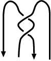
Refer to caption
Figure 5. The clasp tangle C+C^{+}.

We call 𝐜=JC+∈ℋ⊗^​2\mathbf{c}=J_{C^{+}}\in\mathscr{H}^{\hat{\otimes}2} the clasp element for ℋ\mathscr{H}. With ℛ=∑α⊗β=∑α′⊗β′\mathcal{R}=\sum\alpha\otimes\beta=\sum\alpha^{\prime}\otimes\beta^{\prime}, we have

(21) 𝐜=(S​⊗^​id)​(ℛ21​ℛ)=∑S⁡(α)​S​(β′)⊗α′​β.\displaystyle\mathbf{c}=(S\hat{\otimes}\operatorname{id})(\mathcal{R}_{21}\mathcal{R})=\sum S(\alpha)S(\beta^{\prime})\otimes\alpha^{\prime}\beta.

Let C−C^{-} be the mirror image of C+C^{+}, see Figure 6, and 𝐜−=JC−∈ℋ⊗^​2\mathbf{c}^{-}=J_{C^{-}}\in\mathscr{H}^{\hat{\otimes}2}.

Let (C+)′(C^{+})^{\prime} be the tangle obtained by reversing the orientation of the second component of C+C^{+}, and (C+)′′(C^{+})^{\prime\prime} be the result of putting (C+)′(C^{+})^{\prime} on top of the tangle  [Uncaptioned image] , see Figure 6.

Refer to caption
Figure 6. The negative clasp C−C^{-} (on the left) and (C+)′′(C^{+})^{\prime\prime} are isotopic.

By the geometric interpretation of S¯\underline{S}, see [Ha4, Formula 8–10], we have

J(C+)′′=(id⁡⊗^​S¯)​JC+.J_{(C^{+})^{\prime\prime}}=(\operatorname{id}\hat{\otimes}\underline{S})J_{C^{+}}.

Since (C+)′′(C^{+})^{\prime\prime} is isotopic to C−C^{-}, we have

(22) 𝐜−=(id⁡⊗^​S¯)​(𝐜).\displaystyle\mathbf{c}^{-}=(\operatorname{id}\hat{\otimes}\underline{S})(\mathbf{c}).

2.11. Hoste moves

It is known that every integral homology 33-sphere can be obtained by surgery on S3S^{3} along an algebraically split link with ±1\pm 1 framings.

The following refinement of the Kirby–Fenn–Rourke theorem on framed links was first essentially conjectured by Hoste [Ho]. (Hoste stated it in a more general form related to Rolfsen’s calculus for rationally framed links.)

Theorem 2.8 ([Ha6]).

Let LL and L′L^{\prime} be two (non-oriented, non-ordered) algebraically-split ±1\pm 1-framed links in S3S^{3}. Then LL and L′L^{\prime} give orientation-preserving homeomorphic results of surgery if and only if LL and L′L^{\prime} are related by a sequence of ambient isotopy and Hoste moves. Here a Hoste move is a Fenn–Rourke (FR) move between two algebraically-split, ±1\pm 1-framed links, see Figure 7.

Refer to caption
Figure 7. A Hoste move (including the case when there are no vertical strands). Here both these two framed links are algebraically-split and ±1\pm 1-framed.

Theorem 2.8 implies that, to construct an invariant of integral homology spheres, it suffices to construct an invariant of algebraically-split, ±1\pm 1-framed links which is invariant under the Hoste moves.

Lemma 2.9.

Suppose ff is an invariant of oriented, unordered, algebraically-split ±1\pm 1-framed links which is invariant under Hoste moves. Then f⁡(L)f(L) does not depend on the orientation of the link LL. Consequently, ff descends to an invariant of integral homology 3-spheres, i.e. if the results of surgery along two oriented, unordered, algebraically-split ±1\pm 1-framed links LL and L′L^{\prime} are homeomorphic integral homology 3-spheres, then f⁡(L)=f⁡(L′)f(L)=f(L^{\prime}).

Proof.

Suppose KK is a component of LL so that L=L1∪KL=L_{1}\cup K. We will show that ff does not depend on the orientation of KK by induction on the unknotting number of KK.

First assume that KK is an unknot. We first apply the Hoste move to KK, then apply the Hoste move in the reverse way, obtaining L1∪(−K)L_{1}\cup(-K), where −K-K is the orientation-reversal of KK. This shows f⁡(L1∪K)=f⁡(L1∪(−K))f(L_{1}\cup K)=f(L_{1}\cup(-K)).

Suppose KK is an arbitrary knot with positive unknotting number. We can use a Hoste move to realize a self-crossing change of KK, reducing the unknotting number. Induction on the unknotting number shows that ff does not depend on the orientation of KK. ∎

2.12. Definition of the invariant JMJ_{M} for the case when the ground ring is a field

In this subsection, we explain a construction of an invariant of integral homology spheres associated to a ribbon Hopf algebra over a field 𝐤\mathbf{k}, equipped with “full twist forms”. In this section (Section 2.12), and only in this section, we will assume that ℋ\mathscr{H} is a ribbon Hopf algebra over a field 𝐤\mathbf{k}. This assumption simplifies the definition of the invariant.

2.12.1. Full twist forms

Recall that 𝐜=JC+∈ℋ⊗ℋ\mathbf{c}=J_{C^{+}}\in\mathscr{H}\otimes\mathscr{H} is the universal invariant of the clasp bottom tangle, and 𝐫\mathbf{r} is the ribbon element.

A pair of ad-invariant linear functionals 𝒯+,𝒯−:ℋ→𝐤\mathcal{T}_{+},\mathcal{T}_{-}\colon\thinspace\mathscr{H}\rightarrow\mathbf{k} are called full twist forms for ℋ\mathscr{H} if

(23) (𝒯±⊗id)(𝐜)=𝐫±1.\displaystyle(\mathcal{T}_{\pm}\otimes\operatorname{id})(\mathbf{c})=\mathbf{r}^{\pm 1}.

The following lemma essentially shows how the universal link invariant behaves under the Hoste move, if there are full twist forms.

Lemma 2.10.

Suppose that a ribbon Hopf algebra ℋ\mathscr{H} admits full twist forms (𝒯+,𝒯−)(\mathcal{T}_{+},\mathcal{T}_{-}). Let T=T1∪⋯∪TnT=T_{1}\cup\cdots\cup T_{n} be an nn-component bottom tangle (n≥1n\geq 1) such that the first component T1T_{1} of TT is a 11-component trivial bottom tangle (see Figure 8).

Figure 8. The trivial bottom tangle.

Let T′=T2′∪⋯∪Tn′T^{\prime}=T^{\prime}_{2}\cup\cdots\cup T^{\prime}_{n} be the (n−1)(n-1)-component bottom tangle obtained from T∖T1=T2∪⋯∪TnT\setminus T_{1}=T_{2}\cup\cdots\cup T_{n} by surgery along the closure of T1T_{1} with framing ±1\pm 1 (see Figure 9).

. . .tangle t …
Figure 9. (a) The tangle TT. (b) The tangle T′T^{\prime}.

Then we have

(24) JT′=(𝒯±⊗id⊗(n−1))​(JT).\displaystyle J_{T^{\prime}}=(\mathcal{T}_{\pm}\otimes\operatorname{id}^{\otimes(n-1)})(J_{T}).
Proof.

In this proof we use the universal invariant for tangles that are not bottom tangles. For details, see [Ha4, Section 7.3].

If Tp,qT_{p,q} is a (p+q+1)(p+q+1)-component tangle as depicted in Figure 10(a) with p,q≥0p,q\geq 0, then we have

JTp,q=(id⊗id⊗p⊗S⊗q)​(id⊗Δ[p+q])​(𝐜).\displaystyle J_{T_{p,q}}=(\operatorname{id}\otimes\operatorname{id}^{\otimes p}\otimes S^{\otimes q})(\operatorname{id}\otimes\Delta^{[p+q]})(\mathbf{c}).
…………………… T 1 p q p q (b)(a) ∓ 1
Figure 10. (a) The tangle Tp,qT_{p,q}. (b) The tangle Tp,q;±1′T^{\prime}_{p,q;\pm 1}.

The tangle Tp,q;±1′T^{\prime}_{p,q;\pm 1} obtained from Tp,q∖T1T_{p,q}\setminus T_{1} by surgery along the closure of the first component T1T_{1} of Tp,qT_{p,q} with framing ±1\pm 1 (see Figure 10(b)) has the universal invariant

JTp,q;±1′=(id⊗p⊗S⊗q)​Δ[p+q]​(𝐫±1).\displaystyle J_{T^{\prime}_{p,q;\pm 1}}=(\operatorname{id}^{\otimes p}\otimes S^{\otimes q})\Delta^{[p+q]}(\mathbf{r}^{\pm 1}).

Since 𝒯±\mathcal{T}_{\pm} is a full twist form, it follows that

(𝒯±⊗id⊗(p+q))​(JTp,q)=JTp,q′.\displaystyle(\mathcal{T}_{\pm}\otimes\operatorname{id}^{\otimes(p+q)})(J_{T_{p,q}})=J_{T^{\prime}_{p,q}}.

The general case follows from the above case and functoriality of the universal invariant, since TT can be obtained from some Tp,qT_{p,q} by tensoring and composing appropriate tangles. ∎

2.12.2. Invariant of integral homology 3-spheres

We will show here that a ribbon Hopf algebra ℋ\mathscr{H} with full twist forms 𝒯±\mathcal{T}_{\pm} gives rise to an invariant of integral homology spheres.

Suppose TT is an nn-component bottom tangle with zero linking matrix and ε1,…,εn∈{1,−1}\varepsilon_{1},\ldots,\varepsilon_{n}\in\{1,-1\}. Let M=M⁡(T,ε1,…,εn)M=M(T;\varepsilon_{1},\ldots,\varepsilon_{n}) be the oriented 3-manifold obtained by surgery on S3S^{3} along the framed link L=L⁡(T,ε1,…,εn)L=L(T;\varepsilon_{1},\ldots,\varepsilon_{n}), which is the closure link of TT with the framing on the ii-th component switched to εi\varepsilon_{i}. Since LL is an algebraically split link with ±1\pm 1 framing on each component, MM is an integral homology 3-sphere. Every integral homology 3-sphere can be obtained in this way.

Proposition 2.11.

Suppose ℋ\mathscr{H} is a ribbon Hopf algebra with full twist forms 𝒯±\mathcal{T}_{\pm}, and M=M⁡(T,ε1,…,εn)M=M(T;\varepsilon_{1},\ldots,\varepsilon_{n}) is an integral homology 3-sphere. Then

JM:=(𝒯ϵ1⊗⋯⊗𝒯ϵn)​(JT)∈𝐤J_{M}:=(\mathcal{T}_{\epsilon_{1}}\otimes\dots\otimes\mathcal{T}_{\epsilon_{n}})(J_{T})\in\mathbf{k}

is an invariant of MM. In other words, if M⁡(T,ε1,…,εn)≅M⁡(T′,ε1′,…,εn′′)M(T;\varepsilon_{1},\ldots,\varepsilon_{n})\cong M(T^{\prime};\varepsilon^{\prime}_{1},\dots,\varepsilon^{\prime}_{n^{\prime}}), then

(𝒯ϵ1⊗⋯⊗𝒯ϵn)​(JT)=(𝒯ϵ1′⊗⋯⊗𝒯ϵn′′)​(JT′).(\mathcal{T}_{\epsilon_{1}}\otimes\dots\otimes\mathcal{T}_{\epsilon_{n}})(J_{T})=(\mathcal{T}_{\epsilon^{\prime}_{1}}\otimes\dots\otimes\mathcal{T}_{\epsilon^{\prime}_{n^{\prime}}})(J_{T^{\prime}}).
Proof.

Since 𝒯±\mathcal{T}_{\pm} are ad-invariant, (𝒯ϵ1⊗⋯⊗𝒯ϵn)​(JT)(\mathcal{T}_{\epsilon_{1}}\otimes\dots\otimes\mathcal{T}_{\epsilon_{n}})(J_{T}) depends only on ϵ1,…,ϵn\epsilon_{1},\ldots,\epsilon_{n} and the oriented, ordered framed link cl⁡(T)\operatorname{cl}(T), but not on the choice of TT, see e.g. [Ha4, Section 11.1]. This shows (𝒯ϵ1⊗⋯⊗𝒯ϵn)​(JT)(\mathcal{T}_{\epsilon_{1}}\otimes\dots\otimes\mathcal{T}_{\epsilon_{n}})(J_{T}) is an invariant of framed link L⁡(T,ε1,…,εn)L(T;\varepsilon_{1},\dots,\varepsilon_{n}).

We now show that (𝒯ϵ1⊗⋯⊗𝒯ϵn)​(JT)(\mathcal{T}_{\epsilon_{1}}\otimes\dots\otimes\mathcal{T}_{\epsilon_{n}})(J_{T}) does not depend on the order of the components of LL. Suppose L=L⁡(T,ε1,…,εn)L=L(T;\varepsilon_{1},\dots,\varepsilon_{n}) and L′L^{\prime} is the same LL, with the orders of the (i+1)(i+1)-th and (i+2)(i+2)-th switched. Then L′=L⁡(T′,ε1′,…,εn′)L^{\prime}=L(T^{\prime};\varepsilon^{\prime}_{1},\dots,\varepsilon^{\prime}_{n}), where T′T^{\prime} is TT on top of a simple braid of bands which switches the i+1i+1 and i+2i+2 components, see Figure 11. Also, εj′=εj\varepsilon^{\prime}_{j}=\varepsilon_{j} for j≠i+1,i+2j\neq i+1,i+2, and εi+1′=εi+2\varepsilon_{i+1}^{\prime}=\varepsilon_{i+2}, εi+2′=εi+1\varepsilon_{i+2}^{\prime}=\varepsilon_{i+1}.

Refer to caption
Figure 11. Modification of a bottom tangle with a braid of bands.

According to the geometric interpretation of the braiding [Ha4, Proposition 8.1],

JT′=(id⊗i⊗𝝍⊗id⊗n−i−2)​(JT).J_{T^{\prime}}=(\operatorname{id}^{\otimes i}\otimes\boldsymbol{\psi}\otimes\operatorname{id}^{\otimes n-i-2})(J_{T}).

By (17),

𝝍⁡(x⊗y)=∑(β⊳y)⊗(α⊳x), where ​ℛ=∑α⊗β.\boldsymbol{\psi}(x\otimes y)=\sum(\beta\triangleright y)\otimes(\alpha\triangleright x),\quad\text{ where }\mathcal{R}=\sum\alpha\otimes\beta.

Since (ϵ⊗ϵ)​(ℛ)=1(\boldsymbol{\epsilon}\otimes\boldsymbol{\epsilon})(\mathcal{R})=1 and 𝒯±\mathcal{T}_{\pm} are ad-invariant,

(𝒯ϵ1⊗⋯⊗𝒯ϵn)​(JT)=(𝒯ϵ1′⊗⋯⊗𝒯ϵn′)​(JT′).(\mathcal{T}_{\epsilon_{1}}\otimes\dots\otimes\mathcal{T}_{\epsilon_{n}})(J_{T})=(\mathcal{T}_{\epsilon_{1}^{\prime}}\otimes\dots\otimes\mathcal{T}_{\epsilon_{n}^{\prime}})(J_{T^{\prime}}).

Thus, (𝒯ϵ1⊗⋯⊗𝒯ϵn)​(JT)(\mathcal{T}_{\epsilon_{1}}\otimes\dots\otimes\mathcal{T}_{\epsilon_{n}})(J_{T}) is an invariant of oriented, unordered framed links.

By Proposition 2.10, (𝒯ϵ1⊗⋯⊗𝒯ϵn)​(JT)(\mathcal{T}_{\epsilon_{1}}\otimes\dots\otimes\mathcal{T}_{\epsilon_{n}})(J_{T}) is invariant under the Hoste moves. Lemma 2.9 implies that (𝒯ϵ1⊗⋯⊗𝒯ϵn)​(JT)(\mathcal{T}_{\epsilon_{1}}\otimes\dots\otimes\mathcal{T}_{\epsilon_{n}})(J_{T}) descends to an invariant of integral homology 3-spheres. ∎

2.12.3. Examples of full twist forms: Factorizable case

A finite-dimensional, quasitriangular Hopf algebra over a field 𝐤\mathbf{k} is said to be factorizable if the clasp element 𝐜∈ℋ⊗𝐤ℋ\mathbf{c}\in\mathscr{H}\otimes_{\mathbf{k}}\mathscr{H} is non-degenerate in the sense that there exist bases {𝐜′​(i),i∈I}\{\mathbf{c}^{\prime}(i),i\in I\} and {𝐜′′​(i),i∈I}\{\mathbf{c}^{\prime\prime}(i),i\in I\} of ℋ\mathscr{H} such that

𝐜=∑i∈I𝐜′​(i)⊗𝐜′′​(i).\mathbf{c}=\sum_{i\in I}\mathbf{c}^{\prime}(i)\otimes\mathbf{c}^{\prime\prime}(i).

This definition of factorizability is equivalent to the original definition by Reshetikhin and Semenov-Tian-Shansky [RS].

Suppose ℋ\mathscr{H} is a factorizable ribbon Hopf algebra. The non-degeneracy condition shows that there is a unique bilinear form, called the clasp form,

ℒ:ℋ⊗ℋ→𝐤\mathscr{L}\colon\thinspace\mathscr{H}\otimes\mathscr{H}\rightarrow\mathbf{k}

such that for every x∈ℋx\in\mathscr{H},

(25) (ℒ⊗id)(x⊗𝐜)=x,(id⊗ℒ)(𝐜⊗x)=x.\displaystyle(\mathscr{L}\otimes\operatorname{id})(x\otimes\mathbf{c})=x,\quad(\operatorname{id}\otimes\mathscr{L})(\mathbf{c}\otimes x)=x.

Using the ad-invariance of 𝐜\mathbf{c}, one can show that ℒ:ℋ⊗ℋ→𝐤\mathscr{L}\colon\thinspace\mathscr{H}\otimes\mathscr{H}\rightarrow\mathbf{k} is ad-invariant. Since 𝐫±1\mathbf{r}^{\pm 1} are ad-invariant, the form 𝒯±:ℋ→𝐤\mathcal{T}_{\pm}\colon\thinspace\mathscr{H}\to\mathbf{k} defined by

(26) 𝒯±​(x):=ℒ⁡(𝐫±1⊗x),\displaystyle\mathcal{T}_{\pm}(x):=\mathscr{L}(\mathbf{r}^{\pm 1}\otimes x),

is ad-invariant and satisfies (23) due to (25). Hence 𝒯+\mathcal{T}_{+} and 𝒯−\mathcal{T}_{-} are full twist forms for ℋ\mathscr{H}, and defines an invariant of integral homology 3-sphere according to Proposition 2.11.

Remark 2.12.

Given a finite-dimensional, factorizable, ribbon Hopf algebra ℋ\mathscr{H}, one can construct the Hennings invariant for closed 33-manifolds [He, KR, Oht2, Ke, Ly, Sa, Vi, Ha4]. The invariant given in Proposition 2.11 constructed from the full twist forms in (26) is equal to the Hennings invariant.

2.13. Partially defined twist forms and invariant JMJ_{M}

Let us return to the case when ℋ\mathscr{H} is a ribbon Hopf algebra over ℂ⁡[[h]]\mathbb{C}[[h]]. Recall that ℋ\mathscr{H} is a topologically free ℋ\mathscr{H}-module with the adjoint action. In general ℋ\mathscr{H} does not admit full twist forms.

In the construction of the invariant of integral homology 3-spheres in Proposition 2.11, one first constructs the universal invariant of algebraically split tangles JTJ_{T}, then feeds the result to the functionals 𝒯ϵ1⊗⋯⊗𝒯ϵn\mathcal{T}_{\epsilon_{1}}\otimes\cdots\otimes\mathcal{T}_{\epsilon_{n}} which come from the twist forms 𝒯±\mathcal{T}_{\pm}. We will show that the conclusion of Proposition 2.11 holds true if the twist forms 𝒯±\mathcal{T}_{\pm} are defined on a submodule large enough so that the domain of 𝒯ϵ1⊗⋯⊗𝒯ϵn\mathcal{T}_{\epsilon_{1}}\otimes\cdots\otimes\mathcal{T}_{\epsilon_{n}} contains all the values of JTJ_{T}, with TT algebraically split bottom tangles.

2.13.1. Partially defined twist forms

Suppose 𝒳⊂ℋ\mathscr{X}\subset\mathscr{H} is a topologically free ℂ⁡[[h]]\mathbb{C}[[h]]-submodule. By Proposition 2.3 all the natural maps 𝒳⊗n→𝒳⊗^​n→ℋ⊗^​n\mathscr{X}^{\otimes n}\to\mathscr{X}^{\hat{\otimes}n}\to\mathscr{H}^{\hat{\otimes}n} and 𝒳​⊗^​ℋ⊗^​(n−1)→ℋ⊗^​n\mathscr{X}\hat{\otimes}\mathscr{H}^{\hat{\otimes}(n-1)}\to\mathscr{H}^{\hat{\otimes}n} are injective. Hence we will consider 𝒳⊗n\mathscr{X}^{\otimes n}, 𝒳⊗^​n\mathscr{X}^{\hat{\otimes}n}, and 𝒳​⊗^​ℋ⊗^​(n−1)\mathscr{X}\hat{\otimes}\mathscr{H}^{\hat{\otimes}(n-1)} as submodules of ℋ⊗^​n\mathscr{H}^{\hat{\otimes}n}. This will explain the meaning of statements like “𝐜∈𝒳​⊗^​ℋ\mathbf{c}\in\mathscr{X}\hat{\otimes}\mathscr{H}”.

Definition 2.

A twist system 𝒯=(𝒯±,𝒳)\mathcal{T}=(\mathcal{T}_{\pm},\mathscr{X}) of a topological ribbon Hopf algebra ℋ\mathscr{H} consists of a topologically free ℂ⁡[[h]]\mathbb{C}[[h]]-submodule 𝒳⊂ℋ\mathscr{X}\subset\mathscr{H} and a pair of ℂ⁡[[h]]\mathbb{C}[[h]]-linear functionals 𝒯±:𝒳→ℂ⁡[[h]]\mathcal{T}_{\pm}:\mathscr{X}\to\mathbb{C}[[h]] satisfying the following conditions.

(i) 𝒳\mathscr{X} is ad-stable (i.e. 𝒳\mathscr{X} is stable under the adjoint action of ℋ\mathscr{H}) and 𝒯±\mathcal{T}_{\pm} are ad-invariant.

(ii) 𝐜∈𝒳​⊗^​ℋ\mathbf{c}\in\mathscr{X}\hat{\otimes}\mathscr{H}.

(iii) One has

(𝒯±​⊗^​id)​(𝐜)=𝐫±1.(\mathcal{T}_{\pm}\hat{\otimes}\operatorname{id})(\mathbf{c})=\mathbf{r}^{\pm 1}.

Recall that for an nn-component bottom tangle TT with zero linking matrix and ε1,…,εn∈{1,−1}\varepsilon_{1},\ldots,\varepsilon_{n}\in\{1,-1\}, M⁡(T,ε1,…,εn)M(T;\varepsilon_{1},\ldots,\varepsilon_{n}) is the integral homology sphere obtained by surgery on S3S^{3} along the framed link L⁡(T,ε1,…,εn)L(T;\varepsilon_{1},\ldots,\varepsilon_{n}), which is the closure link of TT with the framing on the ii-th component switched to εi\varepsilon_{i}.

Proposition 2.13.

Suppose 𝒯=(𝒯±,𝒳)\mathcal{T}=(\mathcal{T}_{\pm},\mathscr{X}) is a twist system of a topological ribbon Hopf algebra ℋ\mathscr{H} such that JT∈𝒳⊗^​nJ_{T}\in\mathscr{X}^{\hat{\otimes}n} for any nn-component algebraically split 0-framed bottom tangle TT. Let M=M⁡(T,ε1,…,εn)M=M(T;\varepsilon_{1},\ldots,\varepsilon_{n}) be an integral homology 3-sphere. Then

JM:=(𝒯ϵ1​⊗^​…​⊗^​𝒯ϵn)​(JT)∈ℂ⁡[[h]]J_{M}:=(\mathcal{T}_{\epsilon_{1}}\hat{\otimes}\dots\hat{\otimes}\mathcal{T}_{\epsilon_{n}})(J_{T})\in\mathbb{C}[[h]]

is an invariant of MM. In other words, if M⁡(T,ε1,…,εn)=M⁡(T′,ε1′,…,εn′′)M(T;\varepsilon_{1},\ldots,\varepsilon_{n})=M(T^{\prime};\varepsilon^{\prime}_{1},\dots,\varepsilon^{\prime}_{n^{\prime}}), then

(𝒯ϵ1​⊗^​…​⊗^​𝒯ϵn)​(JT)=(𝒯ϵ1′​⊗^​…​⊗^​𝒯ϵn′′)​(JT′).(\mathcal{T}_{\epsilon_{1}}\hat{\otimes}\dots\hat{\otimes}\mathcal{T}_{\epsilon_{n}})(J_{T})=(\mathcal{T}_{\epsilon^{\prime}_{1}}\hat{\otimes}\dots\hat{\otimes}\mathcal{T}_{\epsilon^{\prime}_{n^{\prime}}})(J_{T^{\prime}}).
Proof.

First we show the following claim, which is a refinement of Lemma 2.10.

Claim. Let TT and T′T^{\prime} be tangles as in Lemma 2.10. Then JT∈𝒳​⊗^​ℋ⊗^​(n−1)J_{T}\in{\mathscr{X}\hat{\otimes}\mathscr{H}^{\hat{\otimes}(n-1)}}, and

(27) JT′=(𝒯±​⊗^​id⊗^​(n−1))​(JT)∈ℋ⊗^​(n−1).\displaystyle J_{T^{\prime}}=(\mathcal{T}_{\pm}\hat{\otimes}\operatorname{id}^{\hat{\otimes}(n-1)})(J_{T})\in\mathscr{H}^{\hat{\otimes}(n-1)}.
Proof of Claim.

If Tp,qT_{p,q} is a (p+q+1)(p+q+1)-component tangle as depicted in Figure 10(a) with p,q≥0p,q\geq 0, then we have

JTp,q=(id⁡⊗^​id⊗^​p​⊗^​S⊗^​q)​(id⁡⊗^​Δ[p+q])​(𝐜).\displaystyle J_{T_{p,q}}=(\operatorname{id}\hat{\otimes}\operatorname{id}^{\hat{\otimes}p}\hat{\otimes}S^{\hat{\otimes}q})(\operatorname{id}\hat{\otimes}\Delta^{[p+q]})(\mathbf{c}).

Since 𝐜∈𝒳​⊗^​ℋ\mathbf{c}\in\mathscr{X}\hat{\otimes}\mathscr{H}, we have

JTp,q∈𝒳​⊗^​ℋ⊗^​p+q.J_{T_{p,q}}\in\mathscr{X}\hat{\otimes}\mathscr{H}^{\hat{\otimes}p+q}.

Since TT is obtained from Tp,qT_{p,q} by tensoring and composing appropriate tangles which do not involve the first component, we also have

JT∈𝒳​⊗^​ℋ⊗^​n.J_{T}\in\mathscr{X}\hat{\otimes}\mathscr{H}^{\hat{\otimes}n}.

The remaining part of the proof follows exactly the proof of Proposition 2.10. One first verifies the case of Tp,qT_{p,q} using conditions (ii) and (iii) in the definition of twist system, from which the general case follows. This proves the claim. ∎

Using the ad-invariance of 𝒯±\mathcal{T}_{\pm} and (27), one can repeat verbatim the proof of Proposition 2.11, replacing ⊗\otimes by ⊗^\hat{\otimes} everywhere, to get Proposition 2.13. ∎

2.13.2. Values of the universal invariant of algebraically split tangles

In Proposition 2.13, we need JT∈𝒳⊗^​nJ_{T}\in\mathscr{X}^{\hat{\otimes}n} for an nn-component bottom tangle TT with zero linking matrix. To help proving statement like that, we use the following result.

Let 𝒦n⊂ℋ⊗^​n\mathcal{K}_{n}\subset\mathscr{\mathscr{H}}^{\hat{\otimes}n}, n≥0n\geq 0, be a family of subsets. A ℂ⁡[[h]]{\mathbb{C}}[[h]]-module homomorphism f:𝐔h⊗^​a→𝐔h⊗^​bf\colon\thinspace\mathbf{U}_{h}^{\hat{\otimes}a}\rightarrow\mathbf{U}_{h}^{\hat{\otimes}b}, a,b≥0a,b\geq 0, is said to be (𝒦n)(\mathcal{K}_{n})-admissible if we have

(28) f(i,j)​(𝒦i+j+a)⊂𝒦i+j+b.\displaystyle f_{(i,j)}(\mathcal{K}_{i+j+a})\subset\mathcal{K}_{i+j+b}.

for all i,j≥0i,j\geq 0. Here f(i,j):=id⊗^​i⁡⊗^​f​⊗^​id⊗^​jf_{(i,j)}:=\operatorname{id}^{\hat{\otimes}i}\hat{\otimes}f\hat{\otimes}\operatorname{id}^{\hat{\otimes}j}.

Proposition 2.14 (Cf. Corollary 9.15 of [Ha4]).

Let 𝒦n⊂ℋ⊗^​n\mathcal{K}_{n}\subset\mathscr{H}^{\hat{\otimes}n}, n≥0n\geq 0, be a family of subsets such that

(i) 1ℂ⁡[[h]]∈𝒦01_{{\mathbb{C}}[[h]]}\in\mathcal{K}_{0}, 1ℋ∈𝒦11_{\mathscr{H}}\in\mathcal{K}_{1}, 𝐛∈𝒦3\mathbf{b}\in\mathcal{K}_{3},

(ii) for x∈𝒦nx\in\mathcal{K}_{n} and y∈𝒦my\in\mathcal{K}_{m} one has x⊗y∈𝒦n+mx\otimes y\in\mathcal{K}_{n+m}, and

(iii) each of 𝛍,𝛙±1,Δ¯,S¯{\boldsymbol{\mu}},{\boldsymbol{\psi}}^{\pm 1},\underline{\Delta},\underline{S} is (𝒦n)(\mathcal{K}_{n})-admissible.

Then, we have JT∈𝒦nJ_{T}\in\mathcal{K}_{n} for any nn-component algebraically split, 00-framed bottom tangle TT.

Here 𝐛∈𝐔h⊗^​3\mathbf{b}\in\mathbf{U}_{h}^{\hat{\otimes}3} is the universal invariant of the Borromean bottom tangle depicted in Figure 12

Refer to caption
Figure 12. The Borromean tangle

.

2.14. Core subalgebra

We define here a core subalgebra of a topological ribbon Hopf algebra, and show that every core subalgebra gives rise to an invariant of integral homology 3-spheres.

In the following we use overline to denote the closure in the hh-adic topology of ℋ⊗^​n\mathscr{H}^{\hat{\otimes}n}.

A topological Hopf subalgebra of a topological Hopf algebra ℋ\mathscr{H} is a ℂ⁡[[h]]\mathbb{C}[[h]]-subalgebra ℋ′⊂ℋ\mathscr{H}^{\prime}\subset\mathscr{H} such that ℋ′\mathscr{H}^{\prime} is topologically free as a ℂ⁡[[h]]\mathbb{C}[[h]]-module and

Δ⁡(ℋ′)⊂ℋ′​⊗^​ℋ′,S±1​(ℋ′)⊂ℋ′.\displaystyle\Delta(\mathscr{H}^{\prime})\subset\mathscr{H}^{\prime}\hat{\otimes}\mathscr{H}^{\prime},\quad S^{\pm 1}(\mathscr{H}^{\prime})\subset\mathscr{H}^{\prime}.

In general, ℋ′\mathscr{H}^{\prime} is not closed in ℋ\mathscr{H}.

Definition 3.

A topological Hopf subalgebra 𝒳⊂ℋ\mathscr{X}\subset\mathscr{H} of a topological ribbon Hopf algebra ℋ\mathscr{H} is called a core subalgebra of ℋ\mathscr{H} if

(i) 𝒳\mathscr{X} is ℋ\mathscr{H}-ad-stable, i.e. it is an ℋ\mathscr{H}-submodule of ℋ\mathscr{H},

(ii) ℛ∈𝒳⊗𝒳¯\mathcal{R}\in\overline{\mathscr{X}\otimes\mathscr{X}} and 𝐠∈𝒳¯\mathbf{g}\in\overline{\mathscr{X}}, and

(iii) The clasp element 𝐜\mathbf{c}, which is contained in 𝒳⊗𝒳¯\overline{\mathscr{X}\otimes\mathscr{X}} by (ii) (see below), has a presentation

(29) 𝐜=∑i∈I𝐜′​(i)⊗𝐜′′​(i),\mathbf{c}=\sum_{i\in I}\mathbf{c}^{\prime}(i)\otimes\mathbf{c}^{\prime\prime}(i),

where each of the two sets {𝐜′​(i)∣i∈I}\{\mathbf{c}^{\prime}(i)\mid i\in I\} and {𝐜′′​(i)∣i∈I}\{\mathbf{c}^{\prime\prime}(i)\mid i\in I\} is

  • •

    0-convergent in ℋ\mathscr{H}, and

  • •

    a topological basis of 𝒳\mathscr{X}.

Some clarifications are in order. As a topological Hopf subalgebra, 𝒳\mathscr{X} is topologically free as a ℂ⁡[[h]]\mathbb{C}[[h]]-module. By Proposition 2.3, all the natural maps 𝒳⊗n→𝒳⊗^​n→ℋ⊗^​n\mathscr{X}^{\otimes n}\to\mathscr{X}^{\hat{\otimes}n}\to\mathscr{H}^{\hat{\otimes}n} are injective. We will consider 𝒳⊗n\mathscr{X}^{\otimes n} as a ℂ⁡[[h]]\mathbb{C}[[h]]-submodule of ℋ⊗^​n\mathscr{H}^{\hat{\otimes}n} in (ii) above when we take its closure in the hh-adic topology of ℋ⊗^​n\mathscr{H}^{\hat{\otimes}n}. Furthermore, since ℛ−1=(S​⊗^​id)​(ℛ)\mathcal{R}^{-1}=(S\hat{\otimes}\operatorname{id})(\mathcal{R}) and 𝐠−1=S⁡(𝐠)\mathbf{g}^{-1}=S(\mathbf{g}), condition (ii) implies that ℛ±1∈𝒳⊗𝒳¯\mathcal{R}^{\pm 1}\in\overline{\mathscr{X}\otimes\mathscr{X}} and 𝐠±1∈𝒳¯\mathbf{g}^{\pm 1}\in\overline{\mathscr{X}}. Since JTJ_{T}, the universal invariant of an nn-component bottom tangle TT, is built from ℛ±1\mathcal{R}^{\pm 1} and 𝐠±1\mathbf{g}^{\pm 1}, condition (ii) implies that JT∈𝒳⊗n¯J_{T}\in\overline{\mathscr{X}^{\otimes n}}. In particular, 𝐜∈𝒳⊗𝒳¯\mathbf{c}\in\overline{\mathscr{X}\otimes\mathscr{X}}.

Remark 2.15.

A core subalgebra has properties similar to, but still different from, those of both a minimal Hopf algebra [Rad] and a factorizable Hopf algebra [RS]. Note that the notions of a minimal algebra and a factorizable algebra were introduced only for the case when the ground ring is a field. Over ℂ⁡[[h]]\mathbb{C}[[h]] the picture is much more complicated. For example, in [Rad] it was shown that a minimal algebra over a field is always finite-dimensional. Here our core algebras are of infinite rank over ℂ⁡[[h]]\mathbb{C}[[h]].

From now on we fix a core subalgebra 𝒳\mathscr{X} of a topological ribbon Hopf algebra ℋ\mathscr{H}.

Lemma 2.16.

Suppose f:ℋ→ℋf:\mathscr{H}\to\mathscr{H} is a ℂ⁡[[h]]\mathbb{C}[[h]]-module homomorphism such that f⁡(𝒳)⊂𝒳f(\mathscr{X})\subset\mathscr{X}. Then f⁡(𝒳¯)⊂𝒳¯f(\overline{\mathscr{X}})\subset\overline{\mathscr{X}}. In particular, 𝒳¯\overline{\mathscr{X}} is ad-stable.

Proof.

Since ff is continuous in the topology of ℋ\mathscr{H}, we have f⁡(𝒳¯)⊂𝒳¯f(\overline{\mathscr{X}})\subset\overline{\mathscr{X}}. ∎

2.14.1. Clasp form associated to a core subalgebra

Suppose 𝒳⊂ℋ\mathscr{X}\subset\mathscr{H} is a core subalgebra with the presentation (29) for 𝐜\mathbf{c}. Since {𝐜′​(i)}\{\mathbf{c}^{\prime}(i)\} is a topological basis of 𝒳\mathscr{X}, every y∈𝒳y\in\mathscr{X} has its coordinates yi′∈ℂ⁡[[h]]y^{\prime}_{i}\in\mathbb{C}[[h]] such that

y=∑i∈Iyi′​𝐜′​(i),y=\sum_{i\in I}y^{\prime}_{i}\mathbf{c}^{\prime}(i),

where (yi′)i∈I(y^{\prime}_{i})_{i\in I} is 0-convergent, i.e. (yi′)i∈I∈(ℂ​[[h]]I)0(y^{\prime}_{i})_{i\in I}\in(\mathbb{C}[[h]]^{I})_{0}. The map y↦(yi′)y\mapsto(y^{\prime}_{i}) is a ℂ⁡[[h]]\mathbb{C}[[h]]-module isomorphism from 𝒳\mathscr{X} to (ℂ​[[h]]I)0(\mathbb{C}[[h]]^{I})_{0}.

The set {𝐜′′​(i)}\{\mathbf{c}^{\prime\prime}(i)\} is a formal basis of 𝒳¯\overline{\mathscr{X}}, which is a formal series ℂ⁡[[h]]\mathbb{C}[[h]]-module. Every x∈𝒳¯x\in\overline{\mathscr{X}} has its coordinates xi′′∈ℂ⁡[[h]]x^{\prime\prime}_{i}\in\mathbb{C}[[h]] such that in the hh-adic topology of ℋ\mathscr{H},

(30) x=∑i∈Ixi′′​𝐜′′​(i),x=\sum_{i\in I}x^{\prime\prime}_{i}\mathbf{c}^{\prime\prime}(i),

where (xi′′)i∈I∈ℂ​[[h]]I(x^{\prime\prime}_{i})_{i\in I}\in\mathbb{C}[[h]]^{I}. The map x↦(xi′′)x\mapsto(x_{i}^{\prime\prime}) is an ℂ⁡[[h]]\mathbb{C}[[h]]-module isomorphism from 𝒳¯\overline{\mathscr{X}} to ℂ​[[h]]I\mathbb{C}[[h]]^{I}.

Define a bilinear form ℒ=⟨.,.⟩:𝒳¯⊗𝒳→ℂ[[h]]\mathscr{L}=\langle.,.\rangle:\overline{\mathscr{X}}\otimes\mathscr{X}\to\mathbb{C}[[h]], called the clasp form, by

⟨x,y⟩:=∑i∈Ixi′′​yi′.\langle x,y\rangle:=\sum_{i\in I}x^{\prime\prime}_{i}\,y^{\prime}_{i}.

The sum on the right hand side is convergent since (yi′)i∈I(y^{\prime}_{i})_{i\in I} is 0-convergent. The bilinear form is defined so that {𝐜′′​(i)}\{\mathbf{c}^{\prime\prime}(i)\} and {𝐜′​(i)}\{\mathbf{c}^{\prime}(i)\} are dual to each other:

(31) ⟨𝐜′′​(i),𝐜′​(j)⟩=δi​j.\langle\mathbf{c}^{\prime\prime}(i),\mathbf{c}^{\prime}(j)\rangle=\delta_{ij}.

By continuity (in the hh-adic topology), ℒ\mathscr{L} extends to a ℂ⁡[[h]]\mathbb{C}[[h]]-module map, also denoted by ℒ\mathscr{L},

ℒ:𝒳¯​⊗^​𝒳→ℂ⁡[[h]].\mathscr{L}:\overline{\mathscr{X}}\hat{\otimes}\mathscr{X}\to\mathbb{C}[[h]].

The following lemma says that the above bilinear form is dual to 𝐜\mathbf{c}.

Lemma 2.17.

(a) One has 𝐜∈(𝒳​⊗^​ℋ)∩(ℋ​⊗^​𝒳)\mathbf{c}\in(\mathscr{X}\hat{\otimes}\mathscr{H})\cap(\mathscr{H}\hat{\otimes}\mathscr{X}).

(b) For every x∈𝒳¯x\in\overline{\mathscr{X}} and y∈𝒳y\in\mathscr{X} one has

(32) (ℒ​⊗^​id)​(x⊗𝐜)\displaystyle(\mathscr{L}\hat{\otimes}\operatorname{id})(x\otimes\mathbf{c}) =x\displaystyle=x
(33) (id⁡⊗^​ℒ)​(𝐜⊗y)\displaystyle(\operatorname{id}\hat{\otimes}\mathscr{L})(\mathbf{c}\otimes y) =y\displaystyle=y
Remark 2.18.

By part (a), 𝐜∈𝒳​⊗^​ℋ\mathbf{c}\in\mathscr{X}\hat{\otimes}\mathscr{H}, hence x⊗𝐜∈𝒳¯​⊗^​𝒳​⊗^​ℋx\otimes\mathbf{c}\in\overline{\mathscr{X}}\hat{\otimes}\mathscr{X}\hat{\otimes}\mathscr{H}. This is the reason why the left hand side of (32) is well-defined as an element of ℋ\mathscr{H}. Similarly the left hand side of (33) is well-defined. With this well-definedness, all the proofs will be the same as in the case of finite-dimensional vector spaces over a field.

Proof.

(a) Since {𝐜′′​(i)}\{\mathbf{c}^{\prime\prime}(i)\} is 0-convergent in ℋ\mathscr{H}, 𝐜=∑i𝐜′​(i)⊗𝐜′′​(i)∈𝒳​⊗^​ℋ\mathbf{c}=\sum_{i}\mathbf{c}^{\prime}(i)\otimes\mathbf{c}^{\prime\prime}(i)\in\mathscr{X}\hat{\otimes}\mathscr{H}. Similarly, 𝐜∈ℋ​⊗^​𝒳\mathbf{c}\in\mathscr{H}\hat{\otimes}\mathscr{X}.

(b) Suppose xx has the presentation (30). By (31), we have

(34) ⟨x,𝐜′​(i)⟩=x′′​(i).\langle x,\mathbf{c}^{\prime}(i)\rangle=x^{\prime\prime}(i).

Thus, we have

(35) x=∑i⟨x,𝐜′​(i)⟩​𝐜′′​(i),x=\sum_{i}\langle x,\mathbf{c}^{\prime}(i)\rangle\,\mathbf{c}^{\prime\prime}(i),

which is (32). The identity (33) is proved similarly. ∎

Because 𝐫±1∈𝒳¯\mathbf{r}^{\pm 1}\in\overline{\mathscr{X}}, one can define the ℂ⁡[[h]]\mathbb{C}[[h]]-module homomorphisms

(36) 𝒯±:𝒳→ℂ⁡[[h]] by𝒯±​(y)=⟨𝐫±1,y⟩.\mathcal{T}_{\pm}:\mathscr{X}\to\mathbb{C}[[h]]\qquad\text{ by}\quad\mathcal{T}_{\pm}(y)=\langle\mathbf{r}^{\pm 1},y\rangle.

Since 𝐜\mathbf{c} is ad-invariant, one can expect the following.

Lemma 2.19.

(a) The clasp form ℒ:𝒳¯​⊗^​𝒳→ℂ⁡[[h]]\mathscr{L}:\overline{\mathscr{X}}\hat{\otimes}\mathscr{X}\to\mathbb{C}[[h]] is ad-invariant, i.e. it is an ℋ\mathscr{H}-module homomorphism.

(b) The maps 𝒯±:𝒳→ℂ⁡[[h]]\mathcal{T}_{\pm}:\mathscr{X}\to\mathbb{C}[[h]] are ad-invariant.

Proof.

(a) By Proposition 2.4(b), ℒ\mathscr{L} is ad-invariant if and only if for every a∈ℋa\in\mathscr{H}, x∈𝒳¯x\in\overline{\mathscr{X}}, and y∈𝒳y\in\mathscr{X},

(37) ⟨a⊳x,y⟩=⟨x,S⁡(a)⊳y⟩,\langle a\triangleright x,y\rangle=\langle x,S(a)\triangleright y\rangle,

which we will prove now.

Since 𝐜=∑i𝐜′​(i)⊗𝐜′′​(i)\mathbf{c}=\sum_{i}\mathbf{c}^{\prime}(i)\otimes\mathbf{c}^{\prime\prime}(i) is ad-invariant, by Proposition 2.4(a),

∑iS⁡(a)⊳𝐜′​(i)⊗𝐜′′​(i)=∑i𝐜′​(i)⊗a⊳𝐜′′​(i).\sum_{i}S(a)\triangleright\mathbf{c}^{\prime}(i)\otimes\mathbf{c}^{\prime\prime}(i)=\sum_{i}\mathbf{c}^{\prime}(i)\otimes a\triangleright\mathbf{c}^{\prime\prime}(i).

Tensoring with xx on the left, and applying ℒ⊗id\mathscr{L}\otimes\operatorname{id},

∑i⟨x,S⁡(a)⊳𝐜′​(i)⟩​𝐜′′​(i)\displaystyle\sum_{i}\langle x,S(a)\triangleright\mathbf{c}^{\prime}(i)\rangle\,\mathbf{c}^{\prime\prime}(i) =∑i⟨x,𝐜′​(i)⟩​a⊳𝐜′′​(i)\displaystyle=\sum_{i}\langle x,\mathbf{c}^{\prime}(i)\rangle\,a\triangleright\mathbf{c}^{\prime\prime}(i)
=∑ix′′​(i)​a⊳𝐜′′​(i)\displaystyle=\sum_{i}x^{\prime\prime}(i)\,a\triangleright\mathbf{c}^{\prime\prime}(i)
=a⊳(∑ix′′​(i)​𝐜′′​(i))=a⊳x.\displaystyle=a\triangleright\left(\sum_{i}x^{\prime\prime}(i)\,\mathbf{c}^{\prime\prime}(i)\right)=a\triangleright x.

Tensoring on the right with 𝐜′​(j)\mathbf{c}^{\prime}(j) then applying ℒ\mathscr{L}, one has

⟨x,S⁡(a)⊳𝐜′​(j)⟩=⟨a⊳x,𝐜′​(j)⟩,\langle x,S(a)\triangleright\mathbf{c}^{\prime}(j)\rangle=\langle a\triangleright x,\mathbf{c}^{\prime}(j)\rangle,

which is (37) with y=𝐜′​(j)y=\mathbf{c}^{\prime}(j). Since {𝐜′​(j)}\{\mathbf{c}^{\prime}(j)\} is a topological basis of 𝒳\mathscr{X}, (37) holds for any y∈𝒳y\in\mathscr{X}.

(b) follows from Proposition 2.4(c). ∎

Proposition 2.20.

Suppose f:ℋ→ℋf:\mathscr{H}\to\mathscr{H} and g:ℋ→ℋg:\mathscr{H}\to\mathscr{H} are ℂ⁡[[h]]\mathbb{C}[[h]]-module isomorphisms such that f⁡(𝒳)=𝒳f(\mathscr{X})=\mathscr{X}, g⁡(𝒳)=𝒳g(\mathscr{X})=\mathscr{X}, and (f​⊗^​g)​(𝐜)=𝐜(f\hat{\otimes}g)(\mathbf{c})=\mathbf{c}. Then g⁡(𝒳¯)=𝒳¯g(\overline{\mathscr{X}})=\overline{\mathscr{X}}, and for every x∈𝒳¯x\in\overline{\mathscr{X}}, y∈𝒳y\in\mathscr{X}, one has

(38) ⟨g⁡(x),f⁡(y)⟩=⟨x,y⟩.\langle g(x),f(y)\rangle=\langle x,y\rangle.
Proof.

By Lemma 2.16, g±1​(𝒳¯)⊂𝒳¯g^{\pm 1}(\overline{\mathscr{X}})\subset\overline{\mathscr{X}}. It follows that g⁡(𝒳¯)=𝒳¯g(\overline{\mathscr{X}})=\overline{\mathscr{X}}. One has

𝐜=∑i𝐜′​(i)⊗𝐜′′​(i)=∑if⁡(𝐜′​(i))⊗g⁡(𝐜′′​(i)).\mathbf{c}=\sum_{i}\mathbf{c}^{\prime}(i)\otimes\mathbf{c}^{\prime\prime}(i)=\sum_{i}f(\mathbf{c}^{\prime}(i))\otimes g(\mathbf{c}^{\prime\prime}(i)).

Since g⁡(x)∈𝒳¯g(x)\in\overline{\mathscr{X}}, one can replace xx by g⁡(x)g(x) in (32),

g⁡(x)\displaystyle g(x) =(ℒ​⊗^​id)​(g⁡(x)⊗𝐜)=∑i(ℒ​⊗^​id)​(g⁡(x)⊗f⁡(𝐜′​(i))⊗g⁡(𝐜′′​(i)))\displaystyle=(\mathscr{L}\hat{\otimes}\operatorname{id})(g(x)\otimes\mathbf{c})=\sum_{i}(\mathscr{L}\hat{\otimes}\operatorname{id})\left(g(x)\otimes f(\mathbf{c}^{\prime}(i))\otimes g(\mathbf{c}^{\prime\prime}(i))\right)
=∑i⟨g⁡(x),f⁡(𝐜′​(i))⟩​g​(𝐜′′​(i))\displaystyle=\sum_{i}\langle g(x),f(\mathbf{c}^{\prime}(i))\rangle\,g(\mathbf{c}^{\prime\prime}(i))
=g⁡(∑i⟨g⁡(x),f⁡(𝐜′​(i))⟩​g​(𝐜′′​(i)))\displaystyle=g\left(\sum_{i}\langle g(x),f(\mathbf{c}^{\prime}(i))\rangle\,g(\mathbf{c}^{\prime\prime}(i))\right)

Injectivity of gg implies

x=∑i⟨g⁡(x),f⁡(𝐜′​(i))⟩​𝐜′′​(i).x=\sum_{i}\langle g(x),f(\mathbf{c}^{\prime}(i))\rangle\,\mathbf{c}^{\prime\prime}(i).

Comparing with (35) we have, for every i∈Ii\in I,

⟨g⁡(x),f⁡(𝐜′​(i))⟩=⟨x,𝐜′​(i)⟩,\langle g(x),f(\mathbf{c}^{\prime}(i))\rangle=\langle x,\mathbf{c}^{\prime}(i)\rangle,

which shows that (38) holds for y=𝐜′​(i)y=\mathbf{c}^{\prime}(i), i∈Ii\in I. Hence, (38) holds for every y∈𝒳y\in\mathscr{X} since {𝐜′​(i)}\{\mathbf{c}^{\prime}(i)\} is a topological basis of 𝒳\mathscr{X}. ∎

2.14.2. Twist system from core subalgebra

Proposition 2.21.

The collection 𝒯=(𝒯±,𝒳)\mathcal{T}=(\mathcal{T}_{\pm},\mathscr{X}) is a twist system for ℋ\mathscr{H}.

Proof.

By definition, 𝒳\mathscr{X} is ad-stable. By Lemma 2.19, 𝒯±\mathcal{T}_{\pm} are ad-invariant. By Lemma 2.17(a), 𝐜∈𝒳​⊗^​ℋ\mathbf{c}\in\mathscr{X}\hat{\otimes}\mathscr{H}. Finally, Identity (32) with x=𝐫±1x=\mathbf{r}^{\pm 1} gives

(𝒯±​⊗^​id)​𝐜=𝐫±1.(\mathcal{T}_{\pm}\hat{\otimes}\operatorname{id})\mathbf{c}=\mathbf{r}^{\pm 1}.

This shows 𝒯=(𝒯±,𝒳)\mathcal{T}=(\mathcal{T}_{\pm},\mathscr{X}) is a twist system. ∎

2.15. From core subalgebra to invariant of integral homology 3-spheres

Theorem 2.22.

Let 𝒳\mathscr{X} be a core subalgebra of a topological ribbon Hopf algebra ℋ\mathscr{H}, with its associated ℋ\mathscr{H}-module homomorphisms 𝒯±:𝒳→ℂ⁡[[h]]\mathcal{T}_{\pm}:\mathscr{X}\to\mathbb{C}[[h]]. Assume TT is an nn-component bottom tangle with 0 linking matrix, εi∈{±1}\varepsilon_{i}\in\{\pm 1\} for i=1,…,ni=1,\dots,n, and M=M⁡(T,ε1,…,εn)M=M(T;\varepsilon_{1},\dots,\varepsilon_{n}) is the integral homology 3-sphere obtained from S3S^{3} by surgery along cl⁡(T)\operatorname{cl}(T), with framing of the ii-th component changed to εi\varepsilon_{i}.

Then JT∈𝒳⊗^​nJ_{T}\in\mathscr{X}^{\hat{\otimes}n}, and

JM:=(𝒯ε1​⊗^​…​⊗^​𝒯εn)​(JT)∈ℂ⁡[[h]]J_{M}:=(\mathcal{T}_{\varepsilon_{1}}\hat{\otimes}\dots\hat{\otimes}\mathcal{T}_{\varepsilon_{n}})(J_{T})\in\mathbb{C}[[h]]

defines an invariant of integral homology 3-spheres.

By Propositions 2.13 and 2.21, to prove Theorem 2.22, it is sufficient to show the following

Proposition 2.23.

Suppose 𝒳\mathscr{X} is a core subalgebra of a topological ribbon Hopf algebra ℋ\mathscr{H} and TT is an nn-component bottom tangle with 0 linking matrix. Then JT∈𝒳⊗^​nJ_{T}\in\mathscr{X}^{\hat{\otimes}n}.

The rest of this section is devoted for a proof of this proposition, based on Proposition 2.14.

2.15.1. (𝒳⊗^​n)(\mathscr{X}^{\hat{\otimes}n})-admissibility

The following lemma follows easily from the definition.

Lemma 2.24.

Suppose f:ℋ⊗^​a→ℋ⊗^​bf:\mathscr{H}^{\hat{\otimes}a}\to\mathscr{H}^{\hat{\otimes}b} is a ℂ⁡[[h]]\mathbb{C}[[h]]-module homomorphism having a presentation as an hh-adically convergent sum f=∑p∈Pfpf=\sum_{p\in P}f_{p} such that for each pp, fp​(𝒳⊗^​a)⊂𝒳⊗^​bf_{p}(\mathscr{X}^{\hat{\otimes}a})\subset\mathscr{X}^{\hat{\otimes}b}, where PP is a countable set. (Here, the sum ff being hh-adically convergent means that for each j≥0j\geq 0 we have fp​(ℋ⊗^​a)⊂hj​ℋ⊗^​bf_{p}(\mathscr{H}^{\hat{\otimes}a})\subset h^{j}\mathscr{H}^{\hat{\otimes}b} for all but finitely many p∈Pp\in P.) Then ff is (𝒳⊗^​n)(\mathscr{X}^{\hat{\otimes}n})-admissible.

Proposition 2.25.

Each of 𝛍,𝛙±1,Δ¯,S¯\boldsymbol{\mu},\boldsymbol{\psi}^{\pm 1},\underline{\Delta},\underline{S} is (𝒳⊗^​n)(\mathscr{X}^{\hat{\otimes}n})-admissible.

Proof.

(a) Because 𝝁⁡(𝒳​⊗^​𝒳)⊂𝒳\boldsymbol{\mu}(\mathscr{X}\hat{\otimes}\mathscr{X})\subset\mathscr{X}, by Lemma 2.24, 𝝁\boldsymbol{\mu} is (𝒳⊗^​n)(\mathscr{X}^{\hat{\otimes}n})-admissible.

(b) Because ℛ∈𝒳⊗𝒳¯\mathcal{R}\in\overline{\mathscr{X}\otimes\mathscr{X}}, ℛ\mathcal{R} has a presentation

ℛ=∑p∈Pℛ1​(p)⊗ℛ2​(p),ℛ1​(p),ℛ2​(p)∈𝒳,\mathcal{R}=\sum_{p\in P}\mathcal{R}_{1}(p)\otimes\mathcal{R}_{2}(p),\quad\mathcal{R}_{1}(p),\mathcal{R}_{2}(p)\in\mathscr{X},

where the sum is convergent in the hh-adic topology of ℋ​⊗^​ℋ\mathscr{H}\hat{\otimes}\mathscr{H}. Using the definitions (17)–(20), we the following presentations as hh-adically convergent sums

𝝍\displaystyle\boldsymbol{\psi} =∑p∈P𝝍p+,\displaystyle=\sum_{p\in P}\boldsymbol{\psi}^{+}_{p},\quad where 𝝍p+​(x⊗y)\displaystyle\boldsymbol{\psi}^{+}_{p}(x\otimes y) =∑ℛ2​(p)⊳y⊗ℛ1​(p)⊳x\displaystyle=\sum\mathcal{R}_{2}(p)\triangleright y\otimes\mathcal{R}_{1}(p)\triangleright x
𝝍−1\displaystyle\boldsymbol{\psi}^{-1} =∑p∈P𝝍p−\displaystyle=\sum_{p\in P}\boldsymbol{\psi}^{-}_{p} where 𝝍p−​(x⊗y)\displaystyle\boldsymbol{\psi}^{-}_{p}(x\otimes y) =∑S⁡(ℛ1​(p))⊳y⊗ℛ2​(p)⊳x\displaystyle=\sum S(\mathcal{R}_{1}(p))\triangleright y\otimes\mathcal{R}_{2}(p)\triangleright x
Δ¯\displaystyle\underline{\Delta} =∑p∈PΔ¯p\displaystyle=\sum_{p\in P}\underline{\Delta}_{p} where Δ¯p​(x)\displaystyle\underline{\Delta}_{p}(x) =∑ℛ2​(p)⊳x(2)⊗ℛ1​x(1)\displaystyle=\sum\mathcal{R}_{2}(p)\triangleright x_{(2)}\otimes\mathcal{R}_{1}x_{(1)}
S¯\displaystyle\underline{S} =∑p∈PS¯p\displaystyle=\sum_{p\in P}\underline{S}_{p} where S¯p​(x)\displaystyle\underline{S}_{p}(x) =∑ℛ2​(p)​S​(ℛ1⊳x).\displaystyle=\sum\mathcal{R}_{2}(p)\,S(\mathcal{R}_{1}\triangleright x).

Since ℛ1​(p),ℛ2​(p)∈𝒳\mathcal{R}_{1}(p),\mathcal{R}_{2}(p)\in\mathscr{X}, which is a topological Hopf algebra, we see that 𝝍p±​(𝒳​⊗^​𝒳)⊂𝒳​⊗^​𝒳\boldsymbol{\psi}^{\pm}_{p}(\mathscr{X}\hat{\otimes}\mathscr{X})\subset\mathscr{X}\hat{\otimes}\mathscr{X}, Δ¯p​(𝒳)⊂𝒳​⊗^​𝒳\underline{\Delta}_{p}(\mathscr{X})\subset\mathscr{X}\hat{\otimes}\mathscr{X}, and S¯p​(𝒳)⊂𝒳\underline{S}_{p}(\mathscr{X})\subset\mathscr{X}. By Lemma (2.24), all 𝝍±1,Δ¯,S¯\boldsymbol{\psi}^{\pm 1},\underline{\Delta},\underline{S} are (𝒳⊗^​n)(\mathscr{X}^{\hat{\otimes}n})-admissible. ∎

2.15.2. Braided commutator and Borromean tangle

We recall from [Ha1, Ha4] the definitions and properties of the braided commutator for a braided Hopf algebra and a formula for universal invariant of the Borromean tangle.

Define the braided commutator Υ:ℋ​⊗^​ℋ→ℋ{\Upsilon}\colon\thinspace\mathscr{H}\hat{\otimes}\mathscr{H}\rightarrow\mathscr{H} (for the braided Hopf algebra ℋ¯\underline{\mathscr{H}}) by

Υ=𝝁[4]​(id⁡⊗^​𝝍​⊗^​id)​(id⁡⊗^​S¯​⊗^​S¯​⊗^​id)​(Δ¯​⊗^​Δ¯).\displaystyle{\Upsilon}={\boldsymbol{\mu}}^{[4]}(\operatorname{id}\hat{\otimes}{\boldsymbol{\psi}}\hat{\otimes}\operatorname{id})(\operatorname{id}\hat{\otimes}\underline{S}\hat{\otimes}\underline{S}\hat{\otimes}\operatorname{id})(\underline{\Delta}\hat{\otimes}\underline{\Delta}).

As noted in [Ha4, Section 9.5], with 𝐜=∑i𝐜′​(i)⊗𝐜′′​(i)\mathbf{c}=\sum_{i}\mathbf{c}^{\prime}(i)\otimes\mathbf{c}^{\prime\prime}(i), we have

(39) 𝐛=∑i,j∈I(id⊗^​2⁡⊗^​Υ)​(𝐜′​(i)⊗𝐜′​(j)⊗𝐜′′​(j)⊗𝐜′′​(i))=∑i,j∈I𝐜′​(i)⊗𝐜′​(j)⊗Υ⁡(𝐜′′​(j)⊗𝐜′′​(i)).\displaystyle\mathbf{b}=\sum_{i,j\in I}(\operatorname{id}^{\hat{\otimes}2}\hat{\otimes}\Upsilon)\left(\mathbf{c}^{\prime}(i)\otimes\mathbf{c}^{\prime}(j)\otimes\mathbf{c}^{\prime\prime}(j)\otimes\mathbf{c}^{\prime\prime}(i)\right)=\sum_{i,j\in I}\mathbf{c}^{\prime}(i)\otimes\mathbf{c}^{\prime}(j)\otimes\Upsilon(\mathbf{c}^{\prime\prime}(j)\otimes\mathbf{c}^{\prime\prime}(i)).

Let 𝐛i,j\mathbf{b}_{i,j} be the (i,j)(i,j)-summand of the right hand side. Then each 𝐛i,j∈𝒳⊗^​3\mathbf{b}_{i,j}\in\mathscr{X}^{\hat{\otimes}3} and 𝐛=∑i,j𝐛i,j\mathbf{b}=\sum_{i,j}\mathbf{b}_{i,j}, with the sum converging in the hh-adic topology of ℋ⊗^​3\mathscr{H}^{\hat{\otimes}3}. We want to show that the sum ∑i,j𝐛i,j\sum_{i,j}\mathbf{b}_{i,j} is convergent in the hh-adic topology of 𝒳⊗^​3\mathscr{X}^{\hat{\otimes}3}.

2.15.3. Two definitions of braided commutator

From [Ha4, Section 9.3], we have

(40) Υ\displaystyle{\Upsilon} =𝝁⁡(ad​⊗^​id)​(id⁡⊗^​(S¯​⊗^​id)​Δ¯)\displaystyle={\boldsymbol{\mu}}(\mathrm{ad}\hat{\otimes}\operatorname{id})(\operatorname{id}\hat{\otimes}(\underline{S}\hat{\otimes}\operatorname{id})\underline{\Delta})
(41) =𝝁⁡(id⁡⊗^​adr¯)​((id⁡⊗^​S¯)​Δ¯​⊗^​id),\displaystyle={\boldsymbol{\mu}}(\operatorname{id}\hat{\otimes}\underline{\operatorname{ad^{\mathrm{r}}}})((\operatorname{id}\hat{\otimes}\underline{S})\underline{\Delta}\hat{\otimes}\operatorname{id}),

where adr¯\underline{\operatorname{ad^{\mathrm{r}}}} is the right adjoint action (of the braided Hopf algebra ℋ¯\underline{\mathscr{H}}) defined by

adr¯:=𝝁[3]​(S¯​⊗^​id⁡⊗^​id)​(𝝍​⊗^​id)​(id⁡⊗^​Δ¯).\displaystyle\underline{\operatorname{ad^{\mathrm{r}}}}:={\boldsymbol{\mu}}^{[3]}(\underline{S}\hat{\otimes}\operatorname{id}\hat{\otimes}\operatorname{id})({\boldsymbol{\psi}}\hat{\otimes}\operatorname{id})(\operatorname{id}\hat{\otimes}\underline{\Delta}).
Lemma 2.26.

For x,y∈ℋx,y\in\mathscr{H}, we have

(42) adr¯​(x⊗y)=S−1​(y)⊳x.\displaystyle\underline{\operatorname{ad^{\mathrm{r}}}}(x\otimes y)=S^{-1}(y)\triangleright x.
Proof.

In what follows we use ℛ=∑ℛ1⊗ℛ2=∑ℛ1′⊗ℛ2′=∑ℛ1′′⊗ℛ2′′=∑ℛ1′′′⊗ℛ2′′′\mathcal{R}=\sum\mathcal{R}_{1}\otimes\mathcal{R}_{2}=\sum\mathcal{R}_{1}^{\prime}\otimes\mathcal{R}_{2}^{\prime}=\sum\mathcal{R}_{1}^{\prime\prime}\otimes\mathcal{R}_{2}^{\prime\prime}=\sum\mathcal{R}_{1}^{\prime\prime\prime}\otimes\mathcal{R}_{2}^{\prime\prime\prime}. One can easily verify

(43) 𝝍⁡(x⊗y):=∑(ℛ2​ℛ2′⊳y)⊗ℛ1​x​S​(ℛ1′).\displaystyle{\boldsymbol{\psi}}(x\otimes y):=\sum(\mathcal{R}_{2}\mathcal{R}_{2}^{\prime}\triangleright y)\otimes\mathcal{R}_{1}\ x\,S(\mathcal{R}_{1}^{\prime}).

We have

adr¯​(x⊗y)=𝝁[3]​(S¯​⊗^​id⁡⊗^​id)​(𝝍​⊗^​id)​(x⊗Δ¯​(y))=∑𝝁[3]​(S¯​⊗^​id⁡⊗^​id)​(𝝍​⊗^​id)​(x⊗y(1)¯⊗y(2)¯)=∑𝝁[3]​(S¯​⊗^​id⁡⊗^​id)​(𝝍⁡(x⊗y(1)¯)⊗y(2)¯)=∑𝝁[3](S¯⊗^id⊗^id)(ℛ2ℛ2′⊳y(1)¯⊗ℛ1xS(ℛ1′)⊗y(2)¯)by (43)=∑𝝁[3]​(S¯​(ℛ2​ℛ2′⊳y(1)¯)⊗ℛ1​x​S​(ℛ1′)⊗y(2)¯)=∑S¯​(ℛ2​ℛ2′⊳y(1)¯)​ℛ1​x​S​(ℛ1′)​y(2)¯,\displaystyle\begin{split}\underline{\operatorname{ad^{\mathrm{r}}}}(x\otimes y)&={\boldsymbol{\mu}}^{[3]}(\underline{S}\hat{\otimes}\operatorname{id}\hat{\otimes}\operatorname{id})({\boldsymbol{\psi}}\hat{\otimes}\operatorname{id})(x\otimes\underline{\Delta}(y))\\ &=\sum{\boldsymbol{\mu}}^{[3]}(\underline{S}\hat{\otimes}\operatorname{id}\hat{\otimes}\operatorname{id})({\boldsymbol{\psi}}\hat{\otimes}\operatorname{id})(x\otimes y_{\underline{(1)}}\otimes y_{\underline{(2)}})\\ &=\sum{\boldsymbol{\mu}}^{[3]}(\underline{S}\hat{\otimes}\operatorname{id}\hat{\otimes}\operatorname{id})({\boldsymbol{\psi}}(x\otimes y_{\underline{(1)}})\otimes y_{\underline{(2)}})\\ &=\sum{\boldsymbol{\mu}}^{[3]}(\underline{S}\hat{\otimes}\operatorname{id}\hat{\otimes}\operatorname{id})(\mathcal{R}_{2}\mathcal{R}_{2}^{\prime}\triangleright y_{\underline{(1)}}\otimes\mathcal{R}_{1}xS(\mathcal{R}_{1}^{\prime})\otimes y_{\underline{(2)}})\quad\text{by \eqref{e37}}\\ &=\sum{\boldsymbol{\mu}}^{[3]}(\underline{S}(\mathcal{R}_{2}\mathcal{R}_{2}^{\prime}\triangleright y_{\underline{(1)}})\otimes\mathcal{R}_{1}xS(\mathcal{R}_{1}^{\prime})\otimes y_{\underline{(2)}})\\ &=\sum\underline{S}(\mathcal{R}_{2}\mathcal{R}_{2}^{\prime}\triangleright y_{\underline{(1)}})\mathcal{R}_{1}xS(\mathcal{R}_{1}^{\prime})y_{\underline{(2)}},\end{split}

where Δ¯​(y)=∑y(1)¯⊗y(2)¯\underline{\Delta}(y)=\sum y_{\underline{(1)}}\otimes y_{\underline{(2)}}. Using

∑y(1)¯⊗y(2)¯=∑(ℛ2′′⊳y(2))⊗ℛ1′′​y(1),\displaystyle\sum y_{\underline{(1)}}\otimes y_{\underline{(2)}}=\sum(\mathcal{R}_{2}^{\prime\prime}\triangleright y_{(2)})\otimes\mathcal{R}_{1}^{\prime\prime}y_{(1)},
S¯​(w)=∑S−1​(ℛ2′′′⊳w)​S​(ℛ1′′′),\displaystyle\underline{S}(w)=\sum S^{-1}(\mathcal{R}_{2}^{\prime\prime\prime}\triangleright w)S(\mathcal{R}_{1}^{\prime\prime\prime}),

we obtain

adr¯​(x⊗y)=∑S¯​(ℛ2​ℛ2′⊳y(1)¯)​ℛ1​x​S​(ℛ1′)​y(2)¯=∑S−1​(ℛ2′′′⊳(ℛ2​ℛ2′⊳(ℛ2′′⊳y(2))))​S​(ℛ1′′′)​ℛ1​x​S​(ℛ1′)​ℛ1′′​y(1)=∑S−1​(ℛ2′′′​ℛ2​ℛ2′​ℛ2′′⊳y(2))​S​(ℛ1′′′)​ℛ1​x​S​(ℛ1′)​ℛ1′′​y(1).\displaystyle\begin{split}\underline{\operatorname{ad^{\mathrm{r}}}}(x\otimes y)&=\sum\underline{S}(\mathcal{R}_{2}\mathcal{R}_{2}^{\prime}\triangleright y_{\underline{(1)}})\mathcal{R}_{1}xS(\mathcal{R}_{1}^{\prime})y_{\underline{(2)}}\\ &=\sum S^{-1}(\mathcal{R}_{2}^{\prime\prime\prime}\triangleright(\mathcal{R}_{2}\mathcal{R}_{2}^{\prime}\triangleright(\mathcal{R}_{2}^{\prime\prime}\triangleright y_{(2)})))S(\mathcal{R}_{1}^{\prime\prime\prime})\mathcal{R}_{1}xS(\mathcal{R}_{1}^{\prime})\mathcal{R}_{1}^{\prime\prime}y_{(1)}\\ &=\sum S^{-1}(\mathcal{R}_{2}^{\prime\prime\prime}\mathcal{R}_{2}\mathcal{R}_{2}^{\prime}\mathcal{R}_{2}^{\prime\prime}\triangleright y_{(2)})S(\mathcal{R}_{1}^{\prime\prime\prime})\mathcal{R}_{1}xS(\mathcal{R}_{1}^{\prime})\mathcal{R}_{1}^{\prime\prime}y_{(1)}.\end{split}

Since ∑ℛ2′′′​ℛ2⊗S⁡(ℛ1′′′)​ℛ1=∑ℛ2′​ℛ2′′⊗S⁡(ℛ1′)​ℛ1′′=ℛ21−1​ℛ21=1⊗1\sum\mathcal{R}_{2}^{\prime\prime\prime}\mathcal{R}_{2}\otimes S(\mathcal{R}_{1}^{\prime\prime\prime})\mathcal{R}_{1}=\sum\mathcal{R}_{2}^{\prime}\mathcal{R}_{2}^{\prime\prime}\otimes S(\mathcal{R}_{1}^{\prime})\mathcal{R}_{1}^{\prime\prime}=\mathcal{R}_{21}^{-1}\mathcal{R}_{21}=1\otimes 1, we obtain

adr¯​(x⊗y)=∑S−1​(y(2))​x​y(1)=S−1​(y)⊳x.\displaystyle\begin{split}\underline{\operatorname{ad^{\mathrm{r}}}}(x\otimes y)&=\sum S^{-1}(y_{(2)})xy_{(1)}=S^{-1}(y)\triangleright x.\end{split}

This completes the proof of the lemma. ∎

By Lemma 2.26 and ad⁡(ℋ​⊗^​𝒳)⊂𝒳\mathrm{ad}(\mathscr{H}\hat{\otimes}\mathscr{X})\subset\mathscr{X} we easily obtain

(44) adr¯​(𝒳​⊗^​ℋ)⊂𝒳.\displaystyle\underline{\operatorname{ad^{\mathrm{r}}}}(\mathscr{X}\hat{\otimes}\mathscr{H})\subset\mathscr{X}.
Lemma 2.27.

We have

(45) Υ⁡(ℋ​⊗^​𝒳)⊂𝒳,\displaystyle\Upsilon(\mathscr{H}\hat{\otimes}\mathscr{X})\subset\mathscr{X},
(46) Υ⁡(𝒳​⊗^​ℋ)⊂𝒳.\displaystyle\Upsilon(\mathscr{X}\hat{\otimes}\mathscr{H})\subset\mathscr{X}.
Proof.

Using (40) and ad⁡(ℋ​⊗^​𝒳)⊂𝒳\mathrm{ad}(\mathscr{H}\hat{\otimes}\mathscr{X})\subset\mathscr{X}, we have

Υ⁡(ℋ​⊗^​𝒳)=𝝁⁡(ad​⊗^​id)​(id⁡⊗^​S¯​⊗^​id)​(id⁡⊗^​Δ¯)​(ℋ​⊗^​𝒳)⊂𝝁⁡(ad​⊗^​id)​(id⁡⊗^​S¯​⊗^​id)​(ℋ​⊗^​𝒳​⊗^​𝒳)⊂𝝁⁡(ad​⊗^​id)​(ℋ​⊗^​𝒳​⊗^​𝒳)⊂𝝁⁡(𝒳​⊗^​𝒳)⊂𝒳.\displaystyle\begin{split}\Upsilon(\mathscr{H}\hat{\otimes}\mathscr{X})&={\boldsymbol{\mu}}(\mathrm{ad}\hat{\otimes}\operatorname{id})(\operatorname{id}\hat{\otimes}\underline{S}\hat{\otimes}\operatorname{id})(\operatorname{id}\hat{\otimes}\underline{\Delta})(\mathscr{H}\hat{\otimes}\mathscr{X})\\ &\subset{\boldsymbol{\mu}}(\mathrm{ad}\hat{\otimes}\operatorname{id})(\operatorname{id}\hat{\otimes}\underline{S}\hat{\otimes}\operatorname{id})(\mathscr{H}\hat{\otimes}\mathscr{X}\hat{\otimes}\mathscr{X})\\ &\subset{\boldsymbol{\mu}}(\mathrm{ad}\hat{\otimes}\operatorname{id})(\mathscr{H}\hat{\otimes}\mathscr{X}\hat{\otimes}\mathscr{X})\\ &\subset{\boldsymbol{\mu}}(\mathscr{X}\hat{\otimes}\mathscr{X})\\ &\subset\mathscr{X}.\end{split}

Using (41) and (44), we can similarly check that Υ⁡(𝒳​⊗^​ℋ)⊂𝒳\Upsilon(\mathscr{X}\hat{\otimes}\mathscr{H})\subset\mathscr{X}. ∎

2.15.4. Borromean tangle

Lemma 2.28.

One has 𝐛∈𝒳⊗^​3\mathbf{b}\in\mathscr{X}^{\hat{\otimes}3}.

Proof.

Since {𝐜′′​(i)∣i∈I}\{\mathbf{c}^{\prime\prime}(i)\mid i\in I\} is 0-convergent in ℋ\mathscr{H}, we have 𝐜′′​(i)=hki​𝐜~′′​(i)\mathbf{c}^{\prime\prime}(i)=h^{k_{i}}\tilde{\mathbf{c}}^{\prime\prime}(i), where 𝐜~′′​(i)∈ℋ\tilde{\mathbf{c}}^{\prime\prime}(i)\in\mathscr{H} and for any N≥0N\geq 0 we have ki≥Nk_{i}\geq N for all but finitely many ii.

Recall that, by (39), we have

(47) 𝐛=∑i,j∈I𝐛i,j,where𝐛i,j=𝐜′​(i)⊗𝐜′​(j)⊗Υ⁡(𝐜′′​(i)⊗𝐜′′​(j)).\displaystyle\begin{split}\mathbf{b}&=\sum_{i,j\in I}\mathbf{b}_{i,j},\quad\text{where}\quad\mathbf{b}_{i,j}=\mathbf{c}^{\prime}(i)\otimes\mathbf{c}^{\prime}(j)\otimes\Upsilon(\mathbf{c}^{\prime\prime}(i)\otimes\mathbf{c}^{\prime\prime}(j)).\end{split}

By (45) and (46), we have

Υ⁡(𝐜′′​(i)⊗𝐜′′​(j))=hki​Υ​(𝐜~′′​(i)⊗𝐜′′​(j))∈hki​𝒳,\displaystyle\Upsilon(\mathbf{c}^{\prime\prime}(i)\otimes\mathbf{c}^{\prime\prime}(j))=h^{k_{i}}\Upsilon(\tilde{\mathbf{c}}^{\prime\prime}(i)\otimes\mathbf{c}^{\prime\prime}(j))\in h^{k_{i}}\mathscr{X},
Υ⁡(𝐜′′​(i)⊗𝐜′′​(j))=hkj​Υ​(𝐜′′​(i)⊗𝐜~′′​(j))∈hkj​𝒳,\displaystyle\Upsilon(\mathbf{c}^{\prime\prime}(i)\otimes\mathbf{c}^{\prime\prime}(j))=h^{k_{j}}\Upsilon(\mathbf{c}^{\prime\prime}(i)\otimes\tilde{\mathbf{c}}^{\prime\prime}(j))\in h^{k_{j}}\mathscr{X},

respectively. Hence

(48) Υ⁡(𝐜′′​(i)⊗𝐜′′​(j))∈hmax⁡(ki,kj)​𝒳.\displaystyle\Upsilon(\mathbf{c}^{\prime\prime}(i)\otimes\mathbf{c}^{\prime\prime}(j))\in h^{\max(k_{i},k_{j})}\mathscr{X}.

Since 𝐜′​(i),𝐜′​(j)∈𝒳\mathbf{c}^{\prime}(i),\mathbf{c}^{\prime}(j)\in\mathscr{X}, the sum (47) defines an element of 𝒳⊗^​3\mathscr{X}^{\hat{\otimes}3}. ∎

2.15.5. Proof of Proposition 2.23

It is clear that 1∈𝒳0=ℂ⁡[[h]]1\in\mathscr{X}^{0}=\mathbb{C}[[h]], 1∈𝒳1\in\mathscr{X}, and 𝒳⊗^​n⊗𝒳⊗^​m⊂𝒳⊗^​n+m\mathscr{X}^{\hat{\otimes}n}\otimes\mathscr{X}^{\hat{\otimes}m}\subset\mathscr{X}^{\hat{\otimes}n+m}. By Proposition 2.25, each of 𝝁,𝝍±1,Δ¯,S¯\boldsymbol{\mu},\boldsymbol{\psi}^{\pm 1},\underline{\Delta},\underline{S} is (𝒳⊗^​n)(\mathscr{X}^{\hat{\otimes}n})-admissible. By Lemma 2.28, 𝐛∈𝒳⊗^​3\mathbf{b}\in\mathscr{X}^{\hat{\otimes}3}. Hence by Proposition 2.14, JT∈𝒳⊗^​nJ_{T}\in\mathscr{X}^{\hat{\otimes}n}.

This completes the proof of Proposition 2.23 and also the proof of Theorem 2.22.

2.16. Integrality of JMJ_{M}

Theorem 2.29.

Suppose 𝒳\mathscr{X} is a core subalgebra of a topological ribbon Hopf algebra ℋ\mathscr{H} with the associate twist system 𝒯±:𝒳→ℂ⁡[[h]]\mathcal{T}_{\pm}:\mathscr{X}\to\mathbb{C}[[h]]. Assume that there is a family of subsets 𝒦~n⊂𝒳⊗^​n\widetilde{\mathcal{K}}_{n}\subset\mathscr{\mathscr{X}}^{\hat{\otimes}n}, n≥0n\geq 0, such that

  • (AL1)

    1ℂ⁡[[h]]∈𝒦~01_{{\mathbb{C}}[[h]]}\in\widetilde{\mathcal{K}}_{0}, 1ℋ∈𝒦~11_{\mathscr{H}}\in\widetilde{\mathcal{K}}_{1}, 𝐛∈𝒦~3\mathbf{b}\in\widetilde{\mathcal{K}}_{3}, each of 𝝍±1,𝝁,Δ¯,S¯{\boldsymbol{\psi}}^{\pm 1},{\boldsymbol{\mu}},\underline{\Delta},\underline{S} is (𝒦~n)(\widetilde{\mathcal{K}}_{n})-admissible, and x⊗y∈𝒦~n+mx\otimes y\in\widetilde{\mathcal{K}}_{n+m} for any x∈𝒦~n,y∈𝒦~mx\in\widetilde{\mathcal{K}}_{n},y\in\widetilde{\mathcal{K}}_{m}.

  • (AL2)

    For any ε1,…,εn∈{±}\varepsilon_{1},\dots,\varepsilon_{n}\in\{\pm\},

    (𝒯ε1​⊗^​…​⊗^​𝒯εn)​(𝒦~n)⊂𝒦~0.(\mathcal{T}_{\varepsilon_{1}}\hat{\otimes}\dots\hat{\otimes}\mathcal{T}_{\varepsilon_{n}})(\widetilde{\mathcal{K}}_{n})\subset\widetilde{\mathcal{K}}_{0}.

Then the invariant JMJ_{M} of integral homology 3-spheres has values in 𝒦~0\widetilde{\mathcal{K}}_{0}.

Proof.

Suppose TT is an nn-component bottom tangle TT with zero linking matrix. By Proposition 2.14, Condition (AL1) implies that JT∈𝒦~nJ_{T}\in\widetilde{\mathcal{K}}_{n}. Condition (AL2) implies that

JM=(𝒯ε1​⊗^​…​⊗^​𝒯εn)​(JT)∈𝒦~0,J_{M}=(\mathcal{T}_{\varepsilon_{1}}\hat{\otimes}\dots\hat{\otimes}\mathcal{T}_{\varepsilon_{n}})\left(J_{T}\right)\in\widetilde{\mathcal{K}}_{0},

where M=M⁡(T,ε1,…,εn)M=M(T;\varepsilon_{1},\dots,\varepsilon_{n}). ∎

In the paper we will construct a core subalgebra 𝒳\mathscr{X} and a sequence of ℤ⁡[q]^\widehat{\mathbb{Z}[q]}-submodules 𝒦~n⊂𝒳⊗^​n\widetilde{\mathcal{K}}_{n}\subset\mathscr{X}^{\hat{\otimes}n} satisfying the assumptions (AL1) and (AL2) of Theorem 2.29 for the quantized universal enveloping algebra (of a simple Lie algebra) with 𝒦~0=ℤ⁡[q]^\widetilde{\mathcal{K}}_{0}=\widehat{\mathbb{Z}[q]}. By Theorem 2.29, the corresponding invariant of integral homology 3-spheres takes values in ℤ⁡[q]^\widehat{{\mathbb{Z}}[q]}. We then show that this invariant specializes to the Witten-Reshetikhin-Turaev invariant at roots of unity. In a sense, the (𝒦~n)(\widetilde{\mathcal{K}}_{n}) form an integral version of the (𝒳⊗^​n)(\mathscr{X}^{\hat{\otimes}n}). The construction of the integral objects 𝒦~n\widetilde{\mathcal{K}}_{n} is much more complicated than that of 𝒳\mathscr{X}.

3. Quantized enveloping algebras

In this section we present basic facts about the quantized enveloping algebras associated to a simple Lie algebra 𝔤\mathfrak{g}: the hh-adic version 𝐔h​(𝔤)\mathbf{U}_{h}(\mathfrak{g}), the qq-version 𝐔q​(𝔤)\mathbf{U}_{q}(\mathfrak{g}) and its simply-connected version 𝐔˘q​(𝔤)\breve{\mathbf{U}}_{q}(\mathfrak{g}). We discuss the well-known braid group actions, various automorphisms of 𝐔q\mathbf{U}_{q}, the universal RR-matrix and ribbon structure, and Poincaré-Birkhoff-Witt bases. New materials include gradings on the quantized enveloping algebras in Section 3.3.2, the mirror automorphism φ\varphi, and a calculation of the clasp element.

3.1. Quantized enveloping algebras 𝐔h\mathbf{U}_{h}, 𝐔q\mathbf{U}_{q}, and 𝐔˘q\breve{\mathbf{U}}_{q}

3.1.1. Simple Lie algebra

Suppose 𝔤\mathfrak{g} is a finite-dimensional, simple Lie algebra over ℂ{\mathbb{C}} of rank ℓ\ell. Fix a Cartan subalgebra 𝔥\mathfrak{h} of 𝔤\mathfrak{g} and a basis Π={α1,…,αℓ}\Pi=\{\alpha_{1},\ldots,\alpha_{\ell}\} of simple roots in the dual space 𝔥∗\mathfrak{h}^{*}. Set 𝔥ℝ∗=ℝ​Π⊂𝔥∗\mathfrak{h}^{*}_{\mathbb{R}}=\mathbb{R}\Pi\subset\mathfrak{h}^{*}. Let Y=ℤ​Π⊂𝔥ℝ∗Y={\mathbb{Z}}\Pi\subset\mathfrak{h}^{*}_{\mathbb{R}} denote the root lattice, Φ⊂Y\Phi\subset Y the set of all roots, and Φ+⊂Φ\Phi_{+}\subset\Phi the set of all positive roots. Denote by tt the number of positive roots, t=|Φ+|t=|\Phi_{+}|. Let (⋅,⋅)(\cdot,\cdot) denote the invariant inner product on 𝔥ℝ∗\mathfrak{h}^{*}_{\mathbb{R}} such that (α,α)=2(\alpha,\alpha)=2 for every short root α\alpha. For α∈Φ\alpha\in\Phi, set dα=(α,α)/2∈{1,2,3}d_{\alpha}=(\alpha,\alpha)/2\in\{1,2,3\}. Let XX be the weight lattice, i.e. X⊂𝔥ℝ∗X\subset\mathfrak{h}^{*}_{\mathbb{R}} is the ℤ\mathbb{Z}-span of the fundamental weights α˘1,…,α˘ℓ∈𝔥ℝ∗\breve{\alpha}_{1},\ldots,\breve{\alpha}_{\ell}\in\mathfrak{h}^{*}_{\mathbb{R}}, which are defined by (α˘i,αj)=δi​j​dαi(\breve{\alpha}_{i},\alpha_{j})=\delta_{ij}d_{\alpha_{i}}.

For γ=∑i=1ℓki​αi∈Y\gamma=\sum_{i=1}^{\ell}k_{i}\alpha_{i}\in Y, let ht⁡(γ)=∑iki\operatorname{ht}(\gamma)=\sum_{i}k_{i}. Let ρ\rho be the half-sum of positive roots, ρ=12​∑α∈Φ+α\rho=\frac{1}{2}\sum_{\alpha\in\Phi_{+}}\alpha. It is known that ρ=∑i=1ℓα˘i\rho=\sum_{i=1}^{\ell}\breve{\alpha}_{i}.

We list all simple Lie algebras and their constants in Table 1.

AℓA_{\ell} BℓB_{\ell} CℓC_{\ell} DℓD_{\ell} E6E_{6} E7E_{7} E8E_{8} F4F_{4} G2G_{2}
dd 11 22 2 1 1 1 1 2 3
DD ℓ+1\ell+1 2 2 4 3 2 1 1 1
h∨h^{\vee} ℓ+1\ell+1 2​ℓ−12\ell-1 ℓ+1\ell+1 2​ℓ−22\ell-2 12 18 30 9 4
Table 1. Constants d,D,h∨d,D,h^{\vee} of simple Lie algebras

3.1.2. Base rings

Let vv be an indeterminate, and set 𝒜:=ℤ⁡[v±1]⊂ℂ⁡(v){\mathcal{A}}:={\mathbb{Z}}[v^{\pm 1}]\subset{\mathbb{C}}(v). We regard 𝒜{\mathcal{A}} also as a subring of ℂ⁡[[h]]{\mathbb{C}}[[h]], with v=exp⁡(h/2)v=\exp(h/2). Set q=v2q=v^{2}.

Remark 3.1.

We will follow mostly Janzen’s book [Ja]. However, our vv, qq and hh are equal to “qq”, “q2q^{2}” and “−h-h”, respectively, of [Ja]. Since q=v2q=v^{2}, one could avoid using either qq or vv. We will use both qq and vv because on the one hand the use of half-integer powers of qq would be cumbersome, and on the other hand we would like to stress that many constructions in quantized enveloping algebras can be done over ℤ⁡[q±1]\mathbb{Z}[q^{\pm 1}].

For α∈Φ\alpha\in\Phi and integers n,k≥0n,k\geq 0, set

vα:=vdα,qα:=qdα=vα2,\displaystyle v_{\alpha}:=v^{d_{\alpha}},\quad q_{\alpha}:=q^{d_{\alpha}}=v_{\alpha}^{2},
[n]α:=vαn−vα−nvα−vα−1,[n]α!:=∏i=1n[i]α,[nk]α:=∏i=1k[n−i+1]α[i]α,\displaystyle[n]_{\alpha}:=\frac{v^{n}_{\alpha}-v^{-n}_{\alpha}}{v_{\alpha}-v^{-1}_{\alpha}},\quad[n]_{\alpha}!:=\prod_{i=1}^{n}[i]_{\alpha},\quad\begin{bmatrix}n\\ k\end{bmatrix}_{\alpha}:=\prod_{i=1}^{k}\frac{[n-i+1]_{\alpha}}{[i]_{\alpha}},
{n}α:=vαn−vα−n,{n}α!:=∏i=1n{i}α.\displaystyle\{n\}_{\alpha}:=v^{n}_{\alpha}-v^{-n}_{\alpha},\quad\{n\}_{\alpha}!:=\prod_{i=1}^{n}\{i\}_{\alpha}.

When α\alpha is a short root, we sometimes suppress the subscript α\alpha in these expressions.

Recall that for n≥0n\geq 0 and for any element xx in a ℤ⁡[q]{\mathbb{Z}}[q]-algebra,

(x,q)n:=∏j=0n−1(1−x​qj).\displaystyle(x;q)_{n}:=\prod_{j=0}^{n-1}(1-xq^{j}).

3.1.3. The algebra 𝐔h\mathbf{U}_{h}

The quantized enveloping algebra 𝐔h=𝐔h​(𝔤)\mathbf{U}_{h}=\mathbf{U}_{h}(\mathfrak{g}) is defined as the hh-adically complete ℂ⁡[[h]]{\mathbb{C}}[[h]]-algebra, topologically generated by Eα,Fα,HαE_{\alpha},F_{\alpha},H_{\alpha} for α∈Π\alpha\in\Pi, subject to the relations

(49) Hα​Hβ=Hβ​Hα,\displaystyle H_{\alpha}H_{\beta}=H_{\beta}H_{\alpha},
(50) Hα​Eβ−Eβ​Hα=(α,β)​Eβ,Hα​Fβ−Fβ​Hα=−(α,β)​Fβ,\displaystyle H_{\alpha}E_{\beta}-E_{\beta}H_{\alpha}=(\alpha,\beta)E_{\beta},\qquad H_{\alpha}F_{\beta}-F_{\beta}H_{\alpha}=-(\alpha,\beta)F_{\beta},
(51) Eα​Fβ−Fβ​Eα=δα​β​Kα−Kα−1vα−vα−1,where ​Kα=exp⁡(h​Hα/2),\displaystyle E_{\alpha}F_{\beta}-F_{\beta}E_{\alpha}=\delta_{\alpha\beta}\frac{K_{\alpha}-K_{\alpha}^{-1}}{v_{\alpha}-v_{\alpha}^{-1}},\quad\text{where }K_{\alpha}=\exp(hH_{\alpha}/2),
(52) ∑s=0r(−1)s​[rs]α​Eαr−s​Eβ​Eαs\displaystyle\sum_{s=0}^{r}(-1)^{s}\begin{bmatrix}r\\ s\end{bmatrix}_{\alpha}\,E_{\alpha}^{r-s}E_{\beta}E_{\alpha}^{s} =0,where ​r=1−(β,α)/dα,\displaystyle=0,\quad\text{where }r=1-(\beta,\alpha)/d_{\alpha},
(53) ∑s=0r(−1)s​[rs]α​Fαr−s​Fβ​Fαs\displaystyle\sum_{s=0}^{r}(-1)^{s}\begin{bmatrix}r\\ s\end{bmatrix}_{\alpha}\,F_{\alpha}^{r-s}F_{\beta}F_{\alpha}^{s} =0,where ​r=1−(β,α)/dα.\displaystyle=0,\quad\text{where }r=1-(\beta,\alpha)/d_{\alpha}.

We also write Ei,Fi,KiE_{i},F_{i},K_{i} respectively for Eαi,Fαi,KαiE_{\alpha_{i}},F_{\alpha_{i}},K_{\alpha_{i}}, for i=1,…,ℓi=1,\ldots,\ell.

For every λ=∑α∈Πkα​α∈𝔥ℝ∗\lambda=\sum_{\alpha\in\Pi}k_{\alpha}\alpha\in\mathfrak{h}^{*}_{\mathbb{R}}, define Hλ=∑αkα​HαH_{\lambda}=\sum_{\alpha}{k_{\alpha}}\,H_{\alpha} and Kλ=exp⁡(h2​Hλ)K_{\lambda}=\exp(\frac{h}{2}H_{\lambda}). In particular, one can define K˘α:=Kα˘\breve{K}_{\alpha}:=K_{\breve{\alpha}}, for α∈Π\alpha\in\Pi.

3.1.4. Hopf algebra structure

The algebra 𝐔h\mathbf{U}_{h} has a structure of a complete Hopf algebra over ℂ⁡[[h]]{\mathbb{C}}[[h]], where the comultiplication, counit and antipode are given by:

Δ⁡(Eα)\displaystyle\Delta(E_{\alpha}) =Eα⊗1+Kα⊗Eα,\displaystyle=E_{\alpha}\otimes 1+K_{\alpha}\otimes E_{\alpha}, ϵ⁡(Eα)\displaystyle{\boldsymbol{\epsilon}}(E_{\alpha}) =0,\displaystyle=0, S⁡(Eα)\displaystyle S(E_{\alpha}) =−Kα−1​Eα,\displaystyle=-K_{\alpha}^{-1}E_{\alpha},
Δ⁡(Fα)\displaystyle\Delta(F_{\alpha}) =Fα⊗Kα−1+1⊗Fα,\displaystyle=F_{\alpha}\otimes K_{\alpha}^{-1}+1\otimes F_{\alpha}, ϵ⁡(Fα)\displaystyle{\boldsymbol{\epsilon}}(F_{\alpha}) =0,\displaystyle=0, S⁡(Fα)\displaystyle S(F_{\alpha}) =−Fα​Kα,\displaystyle=-F_{\alpha}K_{\alpha},
Δ⁡(Hα)\displaystyle\Delta(H_{\alpha}) =Hα⊗1+1⊗Hα,\displaystyle=H_{\alpha}\otimes 1+1\otimes H_{\alpha}, ϵ⁡(Hα)\displaystyle{\boldsymbol{\epsilon}}(H_{\alpha}) =0,\displaystyle=0, S⁡(Hα)\displaystyle S(H_{\alpha}) =−Hα.\displaystyle=-H_{\alpha}.

3.1.5. The algebra 𝐔q\mathbf{U}_{q} and its simply-connected version 𝐔˘q\breve{\mathbf{U}}_{q}

Let 𝐔q\mathbf{U}_{q} denote the ℂ⁡(v){\mathbb{C}}(v)-subalgebra of 𝐔h​[h−1]=𝐔h⊗ℂ⁡[h]ℂ⁡[h,h−1]\mathbf{U}_{h}[h^{-1}]=\mathbf{U}_{h}\otimes_{{\mathbb{C}}[h]}{\mathbb{C}}[h,h^{-1}] generated by Eα,FαE_{\alpha},F_{\alpha}, and Kα±1K_{\alpha}^{\pm 1} for all α∈Π\alpha\in\Pi. Alternatively, 𝐔q\mathbf{U}_{q} is defined to be the ℂ⁡(v){\mathbb{C}}(v)-subalgebra generated by the elements KαK_{\alpha}, Kα−1K_{\alpha}^{-1}, EαE_{\alpha}, FαF_{\alpha} (α∈Π\alpha\in\Pi), with relations (51)–(53) and

(54) Kα​Kα−1=Kα−1​Kα=1,\displaystyle K_{\alpha}K_{\alpha}^{-1}=K_{\alpha}^{-1}K_{\alpha}=1,
(55) Kβ​Eα=v(β,α)​Eα​Kβ,Kβ​Fα=v−(β,α)​Eα​Kβ\displaystyle K_{\beta}E_{\alpha}=v^{(\beta,\alpha)}E_{\alpha}K_{\beta},\quad K_{\beta}F_{\alpha}=v^{-(\beta,\alpha)}E_{\alpha}K_{\beta}

for α,β∈Π\alpha,\beta\in\Pi.

The algebra 𝐔q\mathbf{U}_{q} inherits a Hopf algebra structure from 𝐔h​[h−1]\mathbf{U}_{h}[h^{-1}], where

Δ⁡(Kα)=Kα⊗Kα,ϵ⁡(Kα)=1,S⁡(Kα)=Kα−1.\displaystyle\Delta(K_{\alpha})=K_{\alpha}\otimes K_{\alpha},\quad{\boldsymbol{\epsilon}}(K_{\alpha})=1,\quad S(K_{\alpha})=K_{\alpha}^{-1}.

Similarly, the simply-connected version 𝐔˘q\breve{\mathbf{U}}_{q} is the ℂ⁡(v){\mathbb{C}}(v)-subalgebra of 𝐔h​[h−1]\mathbf{U}_{h}[h^{-1}] generated by Eα,FαE_{\alpha},F_{\alpha}, and K˘α±1\breve{K}_{\alpha}^{\pm 1} for all α∈Π\alpha\in\Pi. Again 𝐔˘q\breve{\mathbf{U}}_{q} is a ℂ⁡(v){\mathbb{C}}(v)-Hopf algebra, which contains 𝐔q\mathbf{U}_{q} as a Hopf subalgebra. Let 𝐔˘q0\breve{\mathbf{U}}_{q}^{0} be the ℂ⁡(v){\mathbb{C}}(v)-algebra generated by K˘α±1,α∈Π\breve{K}_{\alpha}^{\pm 1},\alpha\in\Pi. Then

(56) 𝐔˘q=𝐔˘q0​𝐔q.\breve{\mathbf{U}}_{q}=\breve{\mathbf{U}}_{q}^{0}\mathbf{U}_{q}.

The simply-connected version 𝐔˘q\breve{\mathbf{U}}_{q} has been studied in [DKP, Gav, Cal] in connection with quantum adjoint action and various duality results. We need the simply connected version 𝐔˘q​(𝔤)\breve{\mathbf{U}}_{q}(\mathfrak{g}) for a duality result, and also for the description of the RR-matrix.

3.2. Automorphisms

There are unique hh-adically continuous ℂ{\mathbb{C}}-algebra automorphisms ιbar,φ,ω\iota_{\mathrm{bar}},\varphi,\omega of 𝐔h\mathbf{U}_{h} defined by

ιbar​(h)\displaystyle\iota_{\mathrm{bar}}(h) =−h,\displaystyle=-h,\quad ιbar​(Hα)\displaystyle\iota_{\mathrm{bar}}(H_{\alpha}) =Hα,\displaystyle=H_{\alpha},\quad ιbar​(Eα)\displaystyle\iota_{\mathrm{bar}}(E_{\alpha}) =Eα,\displaystyle=E_{\alpha},\quad ιbar​(Fα)\displaystyle\iota_{\mathrm{bar}}(F_{\alpha}) =Fα\displaystyle=F_{\alpha}
ω⁡(h)\displaystyle\omega(h) =h,\displaystyle=h,\quad ω⁡(Hα)\displaystyle\omega(H_{\alpha}) =−Hα,\displaystyle=-H_{\alpha},\quad ω⁡(Eα)\displaystyle\omega(E_{\alpha}) =Fα,\displaystyle=F_{\alpha},\quad ω⁡(Fα)\displaystyle\omega(F_{\alpha}) =Eα\displaystyle=E_{\alpha}
φ⁡(h)\displaystyle\varphi(h) =−h,\displaystyle=-h,\quad φ⁡(Hα)\displaystyle\varphi(H_{\alpha}) =−Hα,\displaystyle=-H_{\alpha},\quad φ⁡(Eα)\displaystyle\varphi(E_{\alpha}) =−Fα​Kα,\displaystyle=-F_{\alpha}K_{\alpha},\quad φ⁡(Fα)\displaystyle\varphi(F_{\alpha}) =−Kα−1​Eα,\displaystyle=-K_{\alpha}^{-1}E_{\alpha},

and a unique hh-adically continuous ℂ{\mathbb{C}}-algebra anti-automorphism τ\tau defined by

τ⁡(h)=h,τ⁡(Hα)=−Hα,τ⁡(Eα)=Eα,τ⁡(Fα)=Fα.\tau(h)=h,\quad\tau(H_{\alpha})=-H_{\alpha},\quad\tau(E_{\alpha})=E_{\alpha},\quad\tau(F_{\alpha})=F_{\alpha}.

The map ιbar\iota_{\mathrm{bar}} is the bar operator of [Lu1], and τ,ω\tau,\omega are the same τ,ω\tau,\omega in [Ja]. All three are involutive, i.e. τ2=ιbar2=ω2=id\tau^{2}=\iota_{\mathrm{bar}}^{2}=\omega^{2}=\operatorname{id}. The restrictions of ιbar,φ,τ,ω\iota_{\mathrm{bar}},\varphi,\tau,\omega to 𝐔h∩𝐔q\mathbf{U}_{h}\cap\mathbf{U}_{q} naturally extend to maps from 𝐔q\mathbf{U}_{q} to 𝐔q\mathbf{U}_{q}, and we have

τ⁡(v)\displaystyle\tau(v) =ω⁡(v)=v,\displaystyle=\omega(v)=v,\quad τ⁡(Kα)\displaystyle\tau(K_{\alpha}) =ω⁡(Kα)=Kα−1,\displaystyle=\omega(K_{\alpha})=K_{\alpha}^{-1},
ιbar​(v)\displaystyle\iota_{\mathrm{bar}}(v) =v−1,\displaystyle=v^{-1},\quad ιbar​(Kα)\displaystyle\iota_{\mathrm{bar}}(K_{\alpha}) =Kα−1,\displaystyle=K_{\alpha}^{-1},
φ⁡(v)\displaystyle\varphi(v) =v−1,\displaystyle=v^{-1},\quad φ⁡(Kα)\displaystyle\varphi(K_{\alpha}) =Kα.\displaystyle=K_{\alpha}.

Unlike ιbar,τ,ω\iota_{\mathrm{bar}},\tau,\omega, the map φ\varphi is a ℂ{\mathbb{C}}-Hopf algebra homomorphism:

Proposition 3.2.

The ℂ{\mathbb{C}}-algebra automorphism φ\varphi commutes with SS and Δ\Delta, i.e.

φ​S=S​φ,(φ​⊗^​φ)​Δ=Δ​φ.\varphi S=S\varphi,\quad(\varphi\hat{\otimes}\varphi)\Delta=\Delta\varphi.

Besides φ=ιbar​τ​ω​S=ιbar​ω​τ​S=S​ιbar​τ​ω\varphi=\iota_{\mathrm{bar}}\tau\omega S=\iota_{\mathrm{bar}}\omega\tau S=S\iota_{\mathrm{bar}}\tau\omega, and

(57) φ2​(x)=S2​(x)=K−2​ρ​x​K2​ρ.\varphi^{2}(x)=S^{2}(x)=K_{-2\rho}xK_{2\rho}.
Proof.

All the statements can be easily checked on generators h,Hα,Eα,Fαh,H_{\alpha},E_{\alpha},F_{\alpha}. ∎

3.3. Gradings by root lattice

3.3.1. YY-grading

There are YY-gradings on 𝐔h\mathbf{U}_{h} and 𝐔q\mathbf{U}_{q} defined by

|Eα|=α,|Fα|=−α,|Hα|=|Kα|=0.\displaystyle|E_{\alpha}|=\alpha,\quad|F_{\alpha}|=-\alpha,\quad|H_{\alpha}|=|K_{\alpha}|=0.

For a subset A⊂𝐔hA\subset\mathbf{U}_{h}, denote by Aμ,μ∈YA_{\mu},\mu\in Y, the set of all elements of YY-grading μ\mu in AA.

We frequently use the following simple fact: If xx is YY-homogeneous and β∈Y\beta\in Y, then

(58) Kβ​x=v(β,|x|)​x​Kβ.\displaystyle K_{\beta}\,x=v^{(\beta,|x|)}xK_{\beta}.

In the language of representation theory, x∈𝐔hx\in\mathbf{U}_{h} has YY-grading β∈Y\beta\in Y if and only if it is an element of weight β\beta in the adjoint representation of 𝐔h\mathbf{U}_{h}.

3.3.2. (Y/2​Y)(Y/2Y)-grading and the even part of 𝐔q\mathbf{U}_{q}

Proposition 3.3.

There is a unique (Y/2​Y)(Y/2Y)-grading on the ℂ⁡(v){\mathbb{C}}(v)-algebra 𝐔q\mathbf{U}_{q} satisfying

deg⁡(Kα)≡α,deg⁡(Eα)≡0,deg⁡(Fα)≡α(mod2​Y)\displaystyle\deg(K_{\alpha})\equiv\alpha,\quad\deg(E_{\alpha})\equiv 0,\quad\deg(F_{\alpha})\equiv\alpha\pmod{2Y}

for α∈Π\alpha\in\Pi.

Proof.

Using the defining relations (51)–(55) for 𝐔q\mathbf{U}_{q}, one checks that the (Y/2​Y)(Y/2Y)-grading is well defined. ∎

The degree 00 part of 𝐔q\mathbf{U}_{q} in the (Y/2​Y)(Y/2Y)-grading, which is generated by Kα±2K_{\alpha}^{\pm 2}, EαE_{\alpha} and Fα​KαF_{\alpha}K_{\alpha} for α∈Π\alpha\in\Pi, is called the even part of 𝐔q\mathbf{U}_{q} and denoted by 𝐔qev\mathbf{U}_{q}^{\mathrm{ev}}. Elements of 𝐔qev\mathbf{U}_{q}^{\mathrm{ev}} are said to be even.

For each α∈Y\alpha\in Y, the degree (αmod2​Y)(\alpha\mod 2Y) part of 𝐔q\mathbf{U}_{q} is Kα​𝐔qevK_{\alpha}\mathbf{U}_{q}^{\mathrm{ev}}.

Lemma 3.4.

(a) Suppose μ∈Y\mu\in Y. Let (𝐔qev)μ(\mathbf{U}_{q}^{\mathrm{ev}})_{\mu} be the grading μ\mu part of 𝐔qev\mathbf{U}_{q}^{\mathrm{ev}}. Then

S⁡((𝐔qev)μ)\displaystyle S\left((\mathbf{U}_{q}^{\mathrm{ev}})_{\mu}\right) ⊂Kμ​𝐔qev,\displaystyle\subset K_{\mu}\,\mathbf{U}_{q}^{\mathrm{ev}},
Δ⁡((𝐔qev)μ)\displaystyle\Delta\left((\mathbf{U}_{q}^{\mathrm{ev}})_{\mu}\right) ⊂⨁λ∈YKλ​(𝐔qev)μ−λ⊗(𝐔qev)λ.\displaystyle\subset\bigoplus_{\lambda\in Y}K_{\lambda}\,(\mathbf{U}_{q}^{\mathrm{ev}})_{\mu-\lambda}\otimes(\mathbf{U}_{q}^{\mathrm{ev}})_{\lambda}.

In particular, Δ⁡(𝐔qev)⊂𝐔q⊗𝐔qev\Delta(\mathbf{U}_{q}^{\mathrm{ev}})\subset\mathbf{U}_{q}\otimes\mathbf{U}_{q}^{\mathrm{ev}}.

(b) The adjoint action preserves the even part, i.e. 𝐔q⊳𝐔qev⊂𝐔qev\mathbf{U}_{q}\triangleright\mathbf{U}_{q}^{\mathrm{ev}}\subset\mathbf{U}_{q}^{\mathrm{ev}}.

(c) Each of ιbar,τ\iota_{\mathrm{bar}},\tau, and φ\varphi leaves 𝐔qev\mathbf{U}_{q}^{\mathrm{ev}} stable, i.e. f⁡(𝐔qev)⊂𝐔qevf(\mathbf{U}_{q}^{\mathrm{ev}})\subset\mathbf{U}_{q}^{\mathrm{ev}} for f=ιbar,τ,φf=\iota_{\mathrm{bar}},\tau,\varphi.

Proof.

(a) Suppose x∈(𝐔qev)μx\in(\mathbf{U}_{q}^{\mathrm{ev}})_{\mu}. We have to show that

S⁡(x)\displaystyle S(x) ∈Kμ​𝐔qev,\displaystyle\in K_{\mu}\,\mathbf{U}_{q}^{\mathrm{ev}},
Δ⁡(x)\displaystyle\Delta(x) ∈⨁λ∈YKλ​(𝐔qev)μ−λ⊗(𝐔qev)λ.\displaystyle\in\bigoplus_{\lambda\in Y}K_{\lambda}\,(\mathbf{U}_{q}^{\mathrm{ev}})_{\mu-\lambda}\otimes(\mathbf{U}_{q}^{\mathrm{ev}})_{\lambda}.

If the statements hold for x=x1∈(𝐔qev)μ1x=x_{1}\in(\mathbf{U}_{q}^{\mathrm{ev}})_{\mu_{1}} and x=x2∈(𝐔qev)μ2x=x_{2}\in(\mathbf{U}_{q}^{\mathrm{ev}})_{\mu_{2}}, then they hold for x=x1​x2∈(𝐔qev)μ1+μ2x=x_{1}x_{2}\in(\mathbf{U}_{q}^{\mathrm{ev}})_{\mu_{1}+\mu_{2}}. Since 𝐔qev\mathbf{U}_{q}^{\mathrm{ev}} is generated as an algebra by Kα±2∈(𝐔qev)0K_{\alpha}^{\pm 2}\in(\mathbf{U}_{q}^{\mathrm{ev}})_{0}, Eα∈(𝐔qev)αE_{\alpha}\in(\mathbf{U}_{q}^{\mathrm{ev}})_{\alpha}, and Fα​Kα∈(𝐔qev)−αF_{\alpha}K_{\alpha}\in(\mathbf{U}_{q}^{\mathrm{ev}})_{-\alpha}, it is enough to prove the statements when xx is one of Kα±2,EαK_{\alpha}^{\pm 2},E_{\alpha}, or Fα​KαF_{\alpha}K_{\alpha}. For these special values of xx, the explicit formulas of S⁡(x)S(x) and Δ⁡(x)\Delta(x) are given in subsection 3.1.4, from which the statements follow immediately.

(b) For x∈𝐔qx\in\mathbf{U}_{q}, we have the following explicit formula for the adjoint actions

Kα⊳x\displaystyle K_{\alpha}\triangleright x =Kα​x​Kα−1\displaystyle=K_{\alpha}\,x\,K_{\alpha}^{-1}
(59) Eα⊳x\displaystyle E_{\alpha}\triangleright x =Eα​x−Kα​x​Kα−1​Eα\displaystyle=E_{\alpha}\,x-K_{\alpha}\,x\,K_{\alpha}^{-1}\,E_{\alpha}
Fα⊳x\displaystyle F_{\alpha}\triangleright x =(Fα​x−x​Fα)​Kα.\displaystyle=(F_{\alpha}\,x-x\,F_{\alpha})\,K_{\alpha}.

If xx is even, then all the right hand sides of the above are even. Since 𝐔q\mathbf{U}_{q} is generated by Kα,Eα,FαK_{\alpha},E_{\alpha},F_{\alpha}, we have 𝐔q⊳𝐔qev⊂𝐔qev\mathbf{U}_{q}\triangleright\mathbf{U}_{q}^{\mathrm{ev}}\subset\mathbf{U}_{q}^{\mathrm{ev}}.

(c) One can check directly that each of ιbar,τ\iota_{\mathrm{bar}},\tau, and φ\varphi maps any of the generators Kα±2,Eα,Fα​KαK_{\alpha}^{\pm 2},E_{\alpha},F_{\alpha}K_{\alpha} of 𝐔qev\mathbf{U}_{q}^{\mathrm{ev}} to an element of 𝐔qev\mathbf{U}_{q}^{\mathrm{ev}}. ∎

Remark 3.5.

In Section 6, we refine the Y/2​YY/2Y-grading of the ℂ⁡(v){\mathbb{C}}(v)-algebra 𝐔q\mathbf{U}_{q} to a grading of the ℂ⁡(v){\mathbb{C}}(v)-algebra 𝐔q\mathbf{U}_{q} by a noncommutative ℤ/2​ℤ{\mathbb{Z}}/2{\mathbb{Z}}-extension of Y/2​YY/2Y.

By (56), 𝐔˘q=𝐔˘q0​𝐔q\breve{\mathbf{U}}_{q}=\breve{\mathbf{U}}_{q}^{0}\mathbf{U}_{q}, where 𝐔˘q0=ℂ⁡(v)​[K˘1±1,…,K˘ℓ±1]\breve{\mathbf{U}}_{q}^{0}={\mathbb{C}}(v)[\breve{K}_{1}^{\pm 1},\dots,\breve{K}_{\ell}^{\pm 1}]. Here we set K˘i=K˘αi\breve{K}_{i}=\breve{K}_{\alpha_{i}} for i=1,…,ℓi=1,\dots,\ell. Let 𝐔˘qev,0=ℂ⁡(v)​[K˘1±2,…,K˘ℓ±2]\breve{\mathbf{U}}_{q}^{{\mathrm{ev}},0}={\mathbb{C}}(v)[\breve{K}_{1}^{\pm 2},\dots,\breve{K}_{\ell}^{\pm 2}] and

𝐔˘qev:=𝐔˘qev,0​𝐔qev.\breve{\mathbf{U}}_{q}^{\mathrm{ev}}:=\breve{\mathbf{U}}_{q}^{{\mathrm{ev}},0}\,\mathbf{U}_{q}^{\mathrm{ev}}.
Lemma 3.6.

One has 𝐔˘q⊳𝐔˘qev⊂𝐔˘qev\breve{\mathbf{U}}_{q}\triangleright\breve{\mathbf{U}}_{q}^{\mathrm{ev}}\subset\breve{\mathbf{U}}_{q}^{\mathrm{ev}} and 𝐔˘q⊳𝐔qev⊂𝐔qev\breve{\mathbf{U}}_{q}\triangleright\mathbf{U}_{q}^{\mathrm{ev}}\subset\mathbf{U}_{q}^{\mathrm{ev}}.

Proof.

The proof is similar to that of Lemma 3.4(b). ∎

3.4. Triangular decompositions and their even versions

Let 𝐔h+\mathbf{U}_{h}^{+} (resp. 𝐔h−\mathbf{U}_{h}^{-}, 𝐔h0\mathbf{U}_{h}^{0}) be the hh-adically closed ℂ⁡[[h]]{\mathbb{C}}[[h]]-subalgebra of 𝐔h\mathbf{U}_{h} topologically generated by EαE_{\alpha} (resp. FαF_{\alpha}, HαH_{\alpha}) for α∈Π\alpha\in\Pi.

Let 𝐔q+\mathbf{U}_{q}^{+} (resp. 𝐔q−\mathbf{U}_{q}^{-}, 𝐔q0\mathbf{U}_{q}^{0}) denote the ℂ⁡(v){\mathbb{C}}(v)-subalgebra of 𝐔q\mathbf{U}_{q} generated by EαE_{\alpha} (resp. FαF_{\alpha}, Kα±1K_{\alpha}^{\pm 1}) for α∈Π\alpha\in\Pi.

It is known that the multiplication map

𝐔q−⊗𝐔q0⊗𝐔q+⟶𝐔q,x⊗x′⊗x′′↦x​x′​x′′\displaystyle\mathbf{U}_{q}^{-}\otimes\mathbf{U}_{q}^{0}\otimes\mathbf{U}_{q}^{+}\longrightarrow\mathbf{U}_{q},\quad x\otimes x^{\prime}\otimes x^{\prime\prime}\mapsto xx^{\prime}x^{\prime\prime}

is an isomorphism of ℂ⁡(v){\mathbb{C}}(v)-vector spaces. This fact is called the triangular decomposition of 𝐔q\mathbf{U}_{q}. Similarly,

𝐔h−​⊗^​𝐔h0​⊗^​𝐔h+⟶𝐔h,x⊗x′⊗x′′↦x​x′​x′′,\displaystyle\mathbf{U}_{h}^{-}\hat{\otimes}\mathbf{U}_{h}^{0}\hat{\otimes}\mathbf{U}_{h}^{+}\longrightarrow\mathbf{U}_{h},\quad x\otimes x^{\prime}\otimes x^{\prime\prime}\mapsto xx^{\prime}x^{\prime\prime},

is an isomorphism of ℂ⁡[[h]]{\mathbb{C}}[[h]]-modules. These triangular decompositions descend to various subalgebras of 𝐔q\mathbf{U}_{q} and 𝐔h\mathbf{U}_{h} which we will introduce later.

We need also an even version of triangular decomposition for 𝐔qev\mathbf{U}_{q}^{\mathrm{ev}}. Although 𝐔q+⊂𝐔qev\mathbf{U}_{q}^{+}\subset\mathbf{U}_{q}^{\mathrm{ev}}, the negative part 𝐔q−\mathbf{U}_{q}^{-} is not even.

Let 𝐔qev,−:=φ⁡(𝐔q+)\mathbf{U}_{q}^{{\mathrm{ev}},-}:=\varphi(\mathbf{U}_{q}^{+}), which is the ℂ⁡(v){\mathbb{C}}(v)-subalgebra of 𝐔qev\mathbf{U}_{q}^{\mathrm{ev}} generated by Fα​Kα=−φ⁡(Eα)F_{\alpha}K_{\alpha}=-\varphi(E_{\alpha}), α∈Π\alpha\in\Pi. Then 𝐔qev,−⊂𝐔qev\mathbf{U}_{q}^{{\mathrm{ev}},-}\subset\mathbf{U}_{q}^{\mathrm{ev}}. Let 𝐔qev,0\mathbf{U}_{q}^{{\mathrm{ev}},0} be the even part of 𝐔q0\mathbf{U}_{q}^{0}, i.e.

𝐔qev,0:=𝐔qev∩𝐔q0=ℂ⁡(v)​[K1±2,…,Kℓ±2].\displaystyle\mathbf{U}_{q}^{{\mathrm{ev}},0}:=\mathbf{U}_{q}^{\mathrm{ev}}\cap\mathbf{U}_{q}^{0}={\mathbb{C}}(v)[K_{1}^{\pm 2},\dots,K_{\ell}^{\pm 2}].

Using (58), we obtain the following isomorphisms of vector spaces

(60) 𝐔qev,−⊗𝐔q0⊗𝐔q+​⟶≅​𝐔q,x⊗y⊗z↦x​y​z.\displaystyle\mathbf{U}_{q}^{{\mathrm{ev}},-}\otimes\mathbf{U}_{q}^{0}\otimes\mathbf{U}_{q}^{+}\overset{\cong}{\longrightarrow}\mathbf{U}_{q},\quad x\otimes y\otimes z\mapsto xyz.
(61) 𝐔qev,−⊗𝐔qev,0⊗𝐔q+​⟶≅​𝐔qev,x⊗y⊗z↦x​y​z.\displaystyle\mathbf{U}_{q}^{{\mathrm{ev}},-}\otimes\mathbf{U}_{q}^{{\mathrm{ev}},0}\otimes\mathbf{U}_{q}^{+}\overset{\cong}{\longrightarrow}\mathbf{U}_{q}^{\mathrm{ev}},\quad x\otimes y\otimes z\mapsto xyz.
(62) 𝐔hev,−⊗𝐔h0⊗𝐔h+​⟶≅​𝐔hev,x⊗y⊗z↦x​y​z.\displaystyle\mathbf{U}_{h}^{{\mathrm{ev}},-}\otimes\mathbf{U}_{h}^{0}\otimes\mathbf{U}_{h}^{+}\overset{\cong}{\longrightarrow}\mathbf{U}_{h}^{\mathrm{ev}},\quad x\otimes y\otimes z\mapsto xyz.

where we set 𝐔hev,−=φ⁡(𝐔h+)\mathbf{U}_{h}^{{\mathrm{ev}},-}=\varphi(\mathbf{U}_{h}^{+}), which is the hh-adically closed ℂ⁡[[h]]{\mathbb{C}}[[h]]-subalgebra of 𝐔h\mathbf{U}_{h} topologically generated by Fα​KαF_{\alpha}K_{\alpha}, α∈Π\alpha\in\Pi. We call (60), (61), and (62) respectively the even triangular decomposition of 𝐔q,𝐔qev\mathbf{U}_{q},\mathbf{U}_{q}^{\mathrm{ev}}, and 𝐔h\mathbf{U}_{h}.

3.5. Braid group action

3.5.1. Braid group and Weyl group

The braid group for the root system Φ\Phi has the presentation with generators TαT_{\alpha} for α∈Π\alpha\in\Pi and with relations

Tα​Tβ=Tβ​Tαfor α,β∈Π, (α,β)=0,\displaystyle T_{\alpha}T_{\beta}=T_{\beta}T_{\alpha}\quad\text{for $\alpha,\beta\in\Pi$, $(\alpha,\beta)=0$},\phantom{-}
Tα​Tβ​Tα=Tβ​Tα​Tβfor α,β∈Π, (α,β)=−1,\displaystyle T_{\alpha}T_{\beta}T_{\alpha}=T_{\beta}T_{\alpha}T_{\beta}\quad\text{for $\alpha,\beta\in\Pi$, $(\alpha,\beta)=-1$},
Tα​Tβ​Tα​Tβ=Tβ​Tα​Tβ​Tαfor α,β∈Π, (α,β)=−2,\displaystyle T_{\alpha}T_{\beta}T_{\alpha}T_{\beta}=T_{\beta}T_{\alpha}T_{\beta}T_{\alpha}\quad\text{for $\alpha,\beta\in\Pi$, $(\alpha,\beta)=-2$},
Tα​Tβ​Tα​Tβ​Tα​Tβ=Tβ​Tα​Tβ​Tα​Tβ​Tαfor α,β∈Π, (α,β)=−3.\displaystyle T_{\alpha}T_{\beta}T_{\alpha}T_{\beta}T_{\alpha}T_{\beta}=T_{\beta}T_{\alpha}T_{\beta}T_{\alpha}T_{\beta}T_{\alpha}\quad\text{for $\alpha,\beta\in\Pi$, $(\alpha,\beta)=-3$}.

The Weyl group 𝔚{\mathfrak{W}} of Φ\Phi is the quotient of braid group by the relations Tα2=1T_{\alpha}^{2}=1 for α∈Π\alpha\in\Pi. We denote the generator in 𝔚{\mathfrak{W}} corresponding to TαT_{\alpha} by sαs_{\alpha}. We set Ti=TαiT_{i}=T_{\alpha_{i}}, si=sαis_{i}=s_{\alpha_{i}} for i=1,…,ℓi=1,\ldots,\ell.

Suppose 𝐢=(i1,…,ik)\mathbf{i}=(i_{1},\ldots,i_{k}) with ij∈{1,2,…,ℓ}i_{j}\in\{1,2,\ldots,\ell\}. Let w(𝐢)=si1si2⋯sik∈𝔚w(\mathbf{i})=s_{i_{1}}s_{i_{2}}\cdots s_{i_{k}}\in{\mathfrak{W}}. If there is no shorter sequence 𝐣\mathbf{j} such that w⁡(𝐢)=w⁡(𝐣)w(\mathbf{i})=w(\mathbf{j}), then we say that the sequence 𝐢\mathbf{i} is reduced, and w⁡(𝐢)w(\mathbf{i}) has length kk. It is known that the length of any reduced sequence is less than or equal to t:=|Φ+|t:=|\Phi_{+}|, the number of positive roots of 𝔤\mathfrak{g}. A sequence 𝐢\mathbf{i} is called longest reduced if 𝐢\mathbf{i} is reduced and has length tt. There is a unique element w0∈𝔚w_{0}\in{\mathfrak{W}} such that for any longest reduced sequence 𝐢\mathbf{i} one has w⁡(𝐢)=w0w(\mathbf{i})=w_{0}.

3.5.2. Braid group action

As described in [Ja, Chapter 8], there is an action of the braid group on the ℂ⁡(v){\mathbb{C}}(v)-algebra 𝐔q\mathbf{U}_{q}. For α∈Π\alpha\in\Pi, Tα:𝐔q→𝐔qT_{\alpha}\colon\mathbf{U}_{q}\rightarrow\mathbf{U}_{q} is ℂ⁡(v){\mathbb{C}}(v)-algebra automorphism defined by

Tα​(Kγ)=Ksα​(γ),Tα​(Eα)=−Fα​Kα,Tα​(Fα)=−Kα−1​Eα,\displaystyle T_{\alpha}(K_{\gamma})=K_{s_{\alpha}(\gamma)},\quad T_{\alpha}(E_{\alpha})=-F_{\alpha}K_{\alpha},\quad T_{\alpha}(F_{\alpha})=-K_{\alpha}^{-1}E_{\alpha},
Tα​(Eβ)\displaystyle T_{\alpha}(E_{\beta}) =∑i=0r(−1)ivα−iEα(r−i)EβEα(i),with r=−(β,α)/dα,\displaystyle=\sum_{i=0}^{r}(-1)^{i}v_{\alpha}^{-i}E_{\alpha}^{(r-i)}E_{\beta}E_{\alpha}^{(i)},\quad\text{with }r=-(\beta,\alpha)/d_{\alpha},
Tα​(Fβ)\displaystyle T_{\alpha}(F_{\beta}) =∑i=0r(−1)ivαiFα(i)FβFα(r−i),with r=−(β,α)/dα,\displaystyle=\sum_{i=0}^{r}(-1)^{i}v_{\alpha}^{i}F_{\alpha}^{(i)}F_{\beta}F_{\alpha}^{(r-i)},\quad\text{with }r=-(\beta,\alpha)/d_{\alpha},

where γ∈Y\gamma\in Y, β∈Π∖{α}\beta\in\Pi\setminus\{\alpha\}. The restriction of TαT_{\alpha} to 𝐔q∩𝐔h\mathbf{U}_{q}\cap\mathbf{U}_{h} extends to a continuous ℂ⁡[[h]]{\mathbb{C}}[[h]]-algebra automorphism TαT_{\alpha} of 𝐔h\mathbf{U}_{h} by setting

Tα​(Hγ)=Hsα​(γ) for γ∈Y.\displaystyle T_{\alpha}(H_{\gamma})=H_{s_{\alpha}(\gamma)}\quad\text{ for $\gamma\in Y$.}
Remark 3.7.

Our TαT_{\alpha} is the same as TαT_{\alpha} of [Ja]. Our Ti=TαiT_{i}=T_{\alpha_{i}} is Ti,1′′T_{i,1}^{\prime\prime} of [Lu1], or T~i−1\tilde{T}_{i}^{-1} of [Lu3].

One can easily check that

(63) Tα±1​(Kβ​𝐔qev)⊂Ksα​(β)​𝐔qev.\displaystyle T_{\alpha}^{\pm 1}(K_{\beta}\mathbf{U}_{q}^{\mathrm{ev}})\subset K_{s_{\alpha}(\beta)}\mathbf{U}_{q}^{\mathrm{ev}}.

for α∈Π\alpha\in\Pi, β∈Y\beta\in Y. In particular, the even part 𝐔qev\mathbf{U}_{q}^{\mathrm{ev}} is stable under Tα±1T_{\alpha}^{\pm 1}. Thus, we have

Proposition 3.8.

The even part 𝐔qev\mathbf{U}_{q}^{\mathrm{ev}} is stable under the action of the braid group.

3.6. PBW type bases

3.6.1. Root vectors

Suppose 𝐢=(i1,…,it)\mathbf{i}=(i_{1},\ldots,i_{t}) is a longest reduced sequence. For j∈{1,…,t}j\in\{1,\ldots,t\}, set

γj=γj(𝐢):=si1si2⋯sij−1(αij).\displaystyle\gamma_{j}=\gamma_{j}(\mathbf{i}):=s_{i_{1}}s_{i_{2}}\cdots s_{i_{j-1}}(\alpha_{i_{j}}).

It is known that γ1,…,γt\gamma_{1},\ldots,\gamma_{t} are distinct positive roots and {γ1,…,γt}=Φ+\{\gamma_{1},\ldots,\gamma_{t}\}=\Phi_{+}. The elements

Eγj(𝐢):=Tαi1Tαi2⋯Tαij−1(Eαij),Fγj(𝐢):=Tαi1Tαi2⋯Tαij−1(Fαij)\displaystyle E_{\gamma_{j}}(\mathbf{i}):=T_{\alpha_{i_{1}}}T_{\alpha_{i_{2}}}\cdots T_{\alpha_{i_{j-1}}}(E_{\alpha_{i_{j}}}),\quad F_{\gamma_{j}}(\mathbf{i}):=T_{\alpha_{i_{1}}}T_{\alpha_{i_{2}}}\cdots T_{\alpha_{i_{j-1}}}(F_{\alpha_{i_{j}}})

are called root vectors corresponding to 𝐢\mathbf{i}. The YY-grading of the root vectors are |Eγj​(𝐢)|=γj=−|Fγj​(𝐢)||E_{\gamma_{j}}(\mathbf{i})|={\gamma_{j}}=-|F_{\gamma_{j}}(\mathbf{i})|. It is known that Eγj​(𝐢)∈𝐔q+E_{\gamma_{j}}(\mathbf{i})\in\mathbf{U}_{q}^{+} and Fγj​(𝐢)∈𝐔q−F_{\gamma_{j}}(\mathbf{i})\in\mathbf{U}_{q}^{-}.

In general, Eγj​(𝐢)E_{\gamma_{j}}(\mathbf{i}) and Fγj​(𝐢)F_{\gamma_{j}}(\mathbf{i}) depend on 𝐢\mathbf{i}, but if γj{\gamma_{j}} is a simple root, i.e. γj=α∈Π{\gamma_{j}}=\alpha\in\Pi, then we have Eγj​(𝐢)=EαE_{\gamma_{j}}(\mathbf{i})=E_{\alpha}, Fγj​(𝐢)=FαF_{\gamma_{j}}(\mathbf{i})=F_{\alpha}.

3.6.2. PBW type bases

Fix a longest reduced sequence 𝐢\mathbf{i}. In what follows, we often suppress 𝐢\mathbf{i} and write Eγ=Eγ​(𝐢)E_{\gamma}=E_{\gamma}(\mathbf{i}), Fγ=Fγ​(𝐢)F_{\gamma}=F_{\gamma}(\mathbf{i}) for all γ∈Φ+\gamma\in\Phi_{+}.

The divided powers Eγ(n)E_{\gamma}^{(n)}, Fγ(n)F_{\gamma}^{(n)} for γ∈Φ+\gamma\in\Phi_{+}, n≥0n\geq 0 are defined by:

Eγ(n):=Eγn/[n]γ!,Fγ(n)=Fγn/[n]γ!.\displaystyle E_{\gamma}^{(n)}:=E_{\gamma}^{n}/[n]_{\gamma}!,\quad F_{\gamma}^{(n)}=F_{\gamma}^{n}/[n]_{\gamma}!.

Following Bourbaki, we denote by ℕ\mathbb{N} the set of non-negative integers. For 𝐧∈ℕt\mathbf{n}\in\mathbb{N}^{t}, define

F(𝐧)=∏←γj∈Φ+Fγj(nj),E(𝐧)=∏←γj∈Φ+Eγj(nj),\displaystyle F^{(\mathbf{n})}=\operatorname{\overleftarrow{\prod}}_{\gamma_{j}\in\Phi_{+}}F_{\gamma_{j}}^{(n_{j})},\qquad E^{(\mathbf{n})}=\operatorname{\overleftarrow{\prod}}_{\gamma_{j}\in\Phi_{+}}E_{\gamma_{j}}^{(n_{j})},\quad

Here ∏←γj∈Φ+\operatorname{\overleftarrow{\prod}}_{\gamma_{j}\in\Phi_{+}} means to take the product in the reverse order of (γ1,γ2,…,γt)(\gamma_{1},\gamma_{2},\dots,\gamma_{t}). For example,

F(𝐧)=∏←γj∈Φ+Fγj(nj)=Fγt(nt)Fγt−1(nt−1)⋯Fγ1(n1).F^{(\mathbf{n})}=\operatorname{\overleftarrow{\prod}}_{\gamma_{j}\in\Phi_{+}}F_{\gamma_{j}}^{(n_{j})}=F_{\gamma_{t}}^{(n_{t})}\,F_{\gamma_{t-1}}^{(n_{t-1})}\cdots F_{\gamma_{1}}^{(n_{1})}.

The set {E(𝐧)∣𝐧∈ℕt}\{E^{(\mathbf{n})}\mid\mathbf{n}\in\mathbb{N}^{t}\} is a basis of the ℂ⁡(v){\mathbb{C}}(v)-vector space 𝐔q+\mathbf{U}_{q}^{+}, and a topological basis of 𝐔h\mathbf{U}_{h}.

Similarly, the set {F(𝐧)∣𝐧∈ℕt}\{F^{(\mathbf{n})}\mid\mathbf{n}\in\mathbb{N}^{t}\} is a basis of 𝐔q−\mathbf{U}_{q}^{-} and a topological basis of 𝐔h−\mathbf{U}_{h}^{-}.

On the other hand, {Kγ∣γ∈Y}\{K_{\gamma}\mid\gamma\in Y\} is a ℂ⁡(v){\mathbb{C}}(v)-basis of 𝐔q0\mathbf{U}_{q}^{0} and {H𝐤∣𝐤∈ℕℓ}\{H^{\mathbf{k}}\mid\mathbf{k}\in\mathbb{N}^{\ell}\}, where H𝐤=∏j=1ℓHjkjH^{\mathbf{k}}=\prod_{j=1}^{\ell}H_{j}^{k_{j}} for 𝐤=(k1,…,kℓ)\mathbf{k}=(k_{1},\dots,k_{\ell}), is a topological basis of 𝐔h0\mathbf{U}_{h}^{0}.

Combining these bases and using the even triangular decompositions (60)–(62), we get the following proposition, which describes the Poincaré-Birkhoff-Witt bases of 𝐔q\mathbf{U}_{q}, 𝐔qev\mathbf{U}_{q}^{\mathrm{ev}}, 𝐔h\mathbf{U}_{h}:

Proposition 3.9.

For any longest reduced sequence 𝐢\mathbf{i},

{F(𝐦)K𝐦KγE(𝐧)∣𝐦,𝐧∈ℕt,γ∈Y} is a ℂ⁡(v)-basis for 𝐔q\displaystyle\{F^{(\mathbf{m})}K_{\mathbf{m}}K_{\gamma}E^{(\mathbf{n})}\mid\mathbf{m},\mathbf{n}\in\mathbb{N}^{t},\gamma\in Y\}\text{ is a ${\mathbb{C}}(v)$-basis for }\mathbf{U}_{q}
{F(𝐦)K𝐦Kγ2E(𝐧)∣𝐦,𝐧∈ℕt,γ∈Y} is a ℂ⁡(v)-basis for 𝐔qev\displaystyle\{F^{(\mathbf{m})}K_{\mathbf{m}}K_{\gamma}^{2}E^{(\mathbf{n})}\mid\mathbf{m},\mathbf{n}\in\mathbb{N}^{t},\gamma\in Y\}\text{ is a ${\mathbb{C}}(v)$-basis for }\mathbf{U}_{q}^{\mathrm{ev}}
{F(𝐦)K𝐦H𝐤E(𝐧)∣𝐦,𝐧∈ℕt,𝐤∈ℕℓ} is a topological basis for 𝐔h.\displaystyle\{F^{(\mathbf{m})}K_{\mathbf{m}}H^{\mathbf{k}}E^{(\mathbf{n})}\mid\mathbf{m},\mathbf{n}\in\mathbb{N}^{t},\mathbf{k}\in\mathbb{N}^{\ell}\}\text{ is a topological basis for }\mathbf{U}_{h}.

where

(64) K𝐧:=∏j=1tKγjnj=K−|F(𝐧)|for 𝐧=(n1,…,nt)∈ℕt.\displaystyle K_{\mathbf{n}}:=\prod_{j=1}^{t}K_{\gamma_{j}}^{n_{j}}=K_{-|F^{(\mathbf{n})}|}\quad\text{for $\mathbf{n}=(n_{1},\ldots,n_{t})\in\mathbb{N}^{t}$.}

3.7. RR-matrix

3.7.1. Quasi-R-matrix

Fix a longest reduced sequence 𝐢\mathbf{i}. Recall that {k}α=vαk−vα−k\{k\}_{\alpha}=v_{\alpha}^{k}-v_{\alpha}^{-k}.

The quasi-R-matrix Θ∈𝐔h⊗^​2\Theta\in\mathbf{U}_{h}^{\hat{\otimes}2} is defined by (see [Ja, Lu1])

(65) Θ=∑𝐧∈ℕtF𝐧⊗E𝐧,\Theta=\sum_{\mathbf{n}\in\mathbb{N}^{t}}F_{\mathbf{n}}\otimes E_{\mathbf{n}},

where for 𝐧=(n1,…,nt)∈ℕt\mathbf{n}=(n_{1},\dots,n_{t})\in\mathbb{N}^{t},

(66) E𝐧\displaystyle E_{\mathbf{n}} :=E(𝐧)​∏j=1t{nj}γj!=∏←γj∈Φ+((vγj−vγj−1)​Eγj)nj,\displaystyle:=E^{(\mathbf{n})}\prod_{j=1}^{t}\{n_{j}\}_{\gamma_{j}}!=\operatorname{\overleftarrow{\prod}}_{\gamma_{j}\in\Phi_{+}}\Big((v_{\gamma_{j}}-v_{\gamma_{j}}^{-1})E_{\gamma_{j}}\Big)^{n_{j}},
(67) F𝐧\displaystyle F_{\mathbf{n}} :=F(𝐧)∏j=1t(−1)njvγj−nj(nj−1)/2=∏←γj∈Φ+(−1)njvγj−nj(nj−1)/2Fγj(nj).\displaystyle:=\,F^{(\mathbf{n})}\prod_{j=1}^{t}(-1)^{n_{j}}v_{\gamma_{j}}^{-n_{j}(n_{j}-1)/2}=\operatorname{\overleftarrow{\prod}}_{\gamma_{j}\in\Phi_{+}}(-1)^{n_{j}}v_{\gamma_{j}}^{-n_{j}(n_{j}-1)/2}\,F_{\gamma_{j}}^{(n_{j})}.

It is known that Θ\Theta does not depend on 𝐢\mathbf{i}, and

(68) Θ−1=(ιbar⊗ιbar)​(Θ)=∑𝐧∈ℕtF𝐧′⊗E𝐧′\displaystyle\Theta^{-1}=(\iota_{\mathrm{bar}}\otimes\iota_{\mathrm{bar}})(\Theta)=\sum_{\mathbf{n}\in\mathbb{N}^{t}}F^{\prime}_{\mathbf{n}}\otimes E^{\prime}_{\mathbf{n}}

where

F𝐧′=ιbar​(F𝐧),E𝐧′=ιbar​(E𝐧).F^{\prime}_{\mathbf{n}}=\iota_{\mathrm{bar}}(F_{\mathbf{n}}),\ E^{\prime}_{\mathbf{n}}=\iota_{\mathrm{bar}}(E_{\mathbf{n}}).

3.7.2. Universal RR-matrix and ribbon element

Define an inner product on 𝔥ℝ=Spanℝ⁡{Hα|α∈Π}\mathfrak{h}_{\mathbb{R}}=\operatorname{Span}_{\mathbb{R}}\{H_{\alpha}\,|\,\alpha\in\Pi\} by (Hα,Hβ)=(α,β)(H_{\alpha},H_{\beta})=(\alpha,\beta). Recall that α˘\breve{\alpha}’s are the fundamental weights. Let H˘α=Hα˘\breve{H}_{\alpha}=H_{\breve{\alpha}}. Then {H˘α/dα,α∈Π}\{\breve{H}_{\alpha}/d_{\alpha},\alpha\in\Pi\} is dual to {Hα,α∈Π}\{H_{\alpha},\alpha\in\Pi\} with respect to the inner product, i.e. (Hα,H˘β/dβ)=δα,β(H_{\alpha},\breve{H}_{\beta}/d_{\beta})=\delta_{\alpha,\beta} for α,β∈Π\alpha,\beta\in\Pi. Define the diagonal part, or the Cartan part, of the RR-matrix by

(69) 𝒟=exp⁡(h2​∑α∈Π(Hα⊗H˘α/dα))∈(𝐔h0)⊗^​2.\displaystyle{\mathcal{D}}=\exp\left(\frac{h}{2}\sum_{\alpha\in\Pi}(H_{\alpha}\otimes\breve{H}_{\alpha}/d_{\alpha})\right)\in(\mathbf{U}_{h}^{0})^{\hat{\otimes}2}.

We have 𝒟=𝒟21{\mathcal{D}}={\mathcal{D}}_{21}, where 𝒟21∈(𝐔h0)⊗^​2{\mathcal{D}}_{21}\in(\mathbf{U}_{h}^{0})^{\hat{\otimes}2} is obtained from 𝒟{\mathcal{D}} by permuting the first and the second tensorands.

A simple calculation shows that, for YY-homogeneous x,y∈𝐔hx,y\in\mathbf{U}_{h}, we have

(70) 𝒟⁡(x⊗y)​𝒟−1=x​K|y|⊗K|x|​y.\displaystyle{\mathcal{D}}(x\otimes y){\mathcal{D}}^{-1}=x\,K_{|y|}\otimes K_{|x|}\,y.

The universal RR-matrix and its inverse are given by

(71) ℛ=𝒟​Θ−1,ℛ−1=Θ​𝒟−1,\mathcal{R}={\mathcal{D}}\Theta^{-1},\quad\mathcal{R}^{-1}=\Theta\,{\mathcal{D}}^{-1},

Note that our RR-matrix is the inverse of the RR-matrix in [Ja].

The quasitriangular Hopf algebra (𝐔h,ℛ)({\mathbf{U}_{h}},\mathcal{R}) has a ribbon element 𝐫\mathbf{r} whose corresponding balanced element (see Section 2.2) is given by 𝐠=K−2​ρ\mathbf{g}=K_{-2\rho}. For YY-homogeneous x∈𝐔hx\in\mathbf{U}_{h} we have

(72) S2​(x)=K−2​ρ​x​K2​ρ=q−(ρ,|x|)​x.\displaystyle S^{2}(x)=K_{-2\rho}xK_{2\rho}=q^{-(\rho,|x|)}x.

With ℛ=∑ℛ1⊗ℛ2\mathcal{R}=\sum\mathcal{R}_{1}\otimes\mathcal{R}_{2}, the ribbon element and its inverse are given by

𝐫=∑S⁡(ℛ1)​K−2​ρ​ℛ2,𝐫−1=∑ℛ1​K2​ρ​ℛ2=∑ℛ2​K−2​ρ​ℛ1.\displaystyle\mathbf{r}=\sum S(\mathcal{R}_{1})K_{-2\rho}\mathcal{R}_{2},\quad\mathbf{r}^{-1}=\sum\mathcal{R}_{1}K_{2\rho}\mathcal{R}_{2}=\sum\mathcal{R}_{2}K_{-2\rho}\mathcal{R}_{1}.

One has 𝐫=JT\mathbf{r}=J_{T} and 𝐫−1=JT′\mathbf{r}^{-1}=J_{T^{\prime}}, where TT and T′T^{\prime} are the bottom tangles in Figure 13.

Refer to caption
Figure 13. Tangles TT (left) and T′T^{\prime} determining the ribbon element 𝐫\mathbf{r} and its inverse

Using (65) and (71), we obtain

(73) 𝐫=∑𝐧∈ℕtF𝐧​K𝐧​𝐫0​E𝐧,𝐫−1=∑𝐧∈ℕtF𝐧′​K𝐧−1​𝐫0−1​E𝐧′\displaystyle\mathbf{r}=\sum_{\mathbf{n}\in\mathbb{N}^{t}}F_{\mathbf{n}}K_{\mathbf{n}}\mathbf{r}_{0}E_{\mathbf{n}},\quad\mathbf{r}^{-1}=\sum_{\mathbf{n}\in\mathbb{N}^{t}}F_{\mathbf{n}}^{\prime}K_{\mathbf{n}}^{-1}\mathbf{r}_{0}^{-1}E_{\mathbf{n}}^{\prime}

where K𝐧K_{\mathbf{n}} is given by (64) and

𝐫0:=K−2​ρ𝝁(𝒟−1)=K−2​ρexp(−h2∑α∈ΠHαH˘α/dα).\mathbf{r}_{0}:=K_{-2\rho}\,{\boldsymbol{\mu}}({\mathcal{D}}^{-1})=K_{-2\rho}\,\exp(-\frac{h}{2}\sum_{\alpha\in\Pi}H_{\alpha}\,\breve{H}_{\alpha}/d_{\alpha}).

We also have

(74) S​(𝐫)=S¯​(𝐫)=𝐫.S(\mathbf{r})=\underline{S}(\mathbf{r})=\mathbf{r}.

3.8. Mirror homomorphism φ\varphi

We defined the ℂ{\mathbb{C}}-algebra homomorphism φ\varphi in Section 3.2.

Proposition 3.10.

The ℂ{\mathbb{C}}-automorphism φ\varphi is a mirror homomorphism for 𝐔h\mathbf{U}_{h}, i.e.

(75) φ⁡(K2​ρ)\displaystyle\varphi(K_{2\rho}) =K2​ρ\displaystyle=K_{2\rho}
(76) (φ​⊗^​φ)​(ℛ)\displaystyle(\varphi\hat{\otimes}\varphi)(\mathcal{R}) =(ℛ−1)21\displaystyle=(\mathcal{R}^{-1})_{21}
(77) (φ​⊗^​φ)2​(ℛ)\displaystyle(\varphi\hat{\otimes}\varphi)^{2}(\mathcal{R}) =ℛ.\displaystyle=\mathcal{R}.

Consequently, if T′T^{\prime} is the mirror image of an nn-component bottom tangle TT, then JT′=φ⊗^​n​(JT)J_{T^{\prime}}=\varphi^{\hat{\otimes}n}(J_{T}).

Proof.

Identity (75) is part of the definition of φ\varphi. One could prove the other two (76) and (77) by direct calculations. Here is an alternative proof using known identities.

By Proposition 3.2, φ=ιbar​ω​τ​S\varphi=\iota_{\mathrm{bar}}\omega\tau S. Hence (76) follows from the following four known identities:

(S​⊗^​S)​(ℛ)\displaystyle(S\hat{\otimes}S)(\mathcal{R}) =ℛby property of R-matrix, Equ. (10)\displaystyle=\mathcal{R}\quad\text{by property of $R$-matrix, Equ. \eqref{eq.SR}}
(τ​⊗^​τ)​ℛ\displaystyle(\tau\hat{\otimes}\tau)\mathcal{R} =(τ⊗^τ)(𝒟Θ−1)=Θ−1𝒟by [Ja, 7.1(2)]\displaystyle=(\tau\hat{\otimes}\tau)({\mathcal{D}}\Theta^{-1})=\Theta^{-1}{\mathcal{D}}\quad\text{by \cite[cite]{[\@@bibref{}{Jantzen}{}{}, 7.1(2)]}}
(ω​⊗^​ω)​(Θ−1​𝒟)\displaystyle(\omega\hat{\otimes}\omega)(\Theta^{-1}{\mathcal{D}}) =Θ21−1𝒟by [Ja, 7.1(3)]\displaystyle=\Theta_{21}^{-1}{\mathcal{D}}\quad\text{by \cite[cite]{[\@@bibref{}{Jantzen}{}{}, 7.1(3)]}}
(ιbar​⊗^​ιbar)​(Θ21−1​𝒟)\displaystyle(\iota_{\mathrm{bar}}\hat{\otimes}\iota_{\mathrm{bar}})(\Theta_{21}^{-1}{\mathcal{D}}) =Θ21𝒟−1=ℛ21−1by (68).\displaystyle=\Theta_{21}{\mathcal{D}}^{-1}=\mathcal{R}_{21}^{-1}\quad\text{by \eqref{e64}}.

Identity (77) follows from (57) and (10):

(φ2​⊗^​φ2)​(ℛ)=(S2⊗S2)​(ℛ)=ℛ.(\varphi^{2}\hat{\otimes}\varphi^{2})(\mathcal{R})=(S^{2}\otimes S^{2})(\mathcal{R})=\mathcal{R}.

This shows φ\varphi is a mirror homomorphism. By Proposition 2.6, JT′=φ⊗^​n​(JT)J_{T^{\prime}}=\varphi^{\hat{\otimes}n}(J_{T}). ∎

Because the negative twist is the mirror image of the positive one, we have the following.

Corollary 3.11.

One has φ⁡(𝐫)=𝐫−1\varphi(\mathbf{r})=\mathbf{r}^{-1}.

3.9. Clasp element and quasi-clasp element

Here we calculate explicitly the value of the clasp element 𝐜=JC+∈𝐔h​⊗^​𝐔h\mathbf{c}=J_{C^{+}}\in\mathbf{U}_{h}\hat{\otimes}\mathbf{U}_{h}, which is the universal invariant of the clasp tangle C+C^{+} of Figure 5. Recall that we have defined E𝐧E_{\mathbf{n}}, F𝐧F_{\mathbf{n}}, and 𝒟{\mathcal{D}} in Section 3.7. We call

(78) Γ:=𝐜​𝒟2\Gamma:=\mathbf{c}{\mathcal{D}}^{2}

the quasi-clasp element. Like the quasi-RR-matrix, the quasi-clasp element enjoy better integrality than the clasp element itself.

Lemma 3.12.

Fix a longest reduced sequence 𝐢\mathbf{i}. We have

(79) 𝐜\displaystyle\mathbf{c} =∑𝐦,𝐧∈ℕtq−(ρ,|E𝐧|)​(F𝐦​K𝐦⊗F𝐧​K𝐧)​(𝒟−2)​(E𝐧⊗E𝐦)\displaystyle=\sum_{\mathbf{m},\mathbf{n}\in{\mathbb{N}^{t}}}q^{-(\rho,|E_{\mathbf{n}}|)}\big(F_{\mathbf{m}}K_{\mathbf{m}}\otimes F_{\mathbf{n}}K_{\mathbf{n}}\big)\,\big({\mathcal{D}}^{-2}\big)\,\big(E_{\mathbf{n}}\otimes E_{\mathbf{m}}\big)
(80) Γ\displaystyle\Gamma =∑𝐦,𝐧∈ℕtq−(ρ,|E𝐧|)+(|E𝐦|,|E𝐧|)​(F𝐦​K𝐦−1​E𝐧⊗F𝐧​K𝐧−1​E𝐦)\displaystyle=\sum_{\mathbf{m},\mathbf{n}\in{\mathbb{N}^{t}}}q^{-(\rho,|E_{\mathbf{n}}|)+(|E_{\mathbf{m}}|,|E_{\mathbf{n}}|)}\big(F_{\mathbf{m}}K_{\mathbf{m}}^{-1}E_{\mathbf{n}}\otimes F_{\mathbf{n}}K_{\mathbf{n}}^{-1}\,E_{\mathbf{m}}\big)
(81) 𝐜\displaystyle\mathbf{c} =(φ⊗S¯−1​φ)​(𝐜).\displaystyle=(\varphi\otimes\underline{S}^{-1}\,\varphi)(\mathbf{c})\,.
Proof.

Let 𝒟−2=∑(𝒟−2)1⊗(𝒟−2)2{\mathcal{D}}^{-2}=\sum({\mathcal{D}}^{-2})_{1}\otimes({\mathcal{D}}^{-2})_{2}, and ℛ−1=∑ℛ¯1⊗ℛ¯2=∑ℛ¯1′⊗ℛ¯2′\mathcal{R}^{-1}=\sum\bar{\mathcal{R}}_{1}\otimes\bar{\mathcal{R}}_{2}=\sum\bar{\mathcal{R}}_{1}^{\prime}\otimes\bar{\mathcal{R}}_{2}^{\prime}. By (21), we obtain

𝐜=∑S⁡(ℛ1)​S​(ℛ2′)⊗ℛ1′​ℛ2=∑ℛ¯1​S2​(ℛ¯2′)⊗ℛ¯1′​ℛ¯2.\displaystyle\begin{split}\mathbf{c}&=\sum S(\mathcal{R}_{1})S(\mathcal{R}_{2}^{\prime})\otimes\mathcal{R}_{1}^{\prime}\mathcal{R}_{2}\\ &=\sum\bar{\mathcal{R}}_{1}S^{2}(\bar{\mathcal{R}}_{2}^{\prime})\otimes\bar{\mathcal{R}}_{1}^{\prime}\bar{\mathcal{R}}_{2}.\end{split}

We have

ℛ−1=Θ​𝒟−1=∑𝐦∈ℕtF𝐦​(𝒟−1)1⊗E𝐦​(𝒟−1)2=∑𝐦∈ℕtF𝐦​K𝐦​(𝒟−1)1⊗(𝒟−1)2​E𝐦.\displaystyle\mathcal{R}^{-1}=\Theta{\mathcal{D}}^{-1}=\sum_{\mathbf{m}\in{\mathbb{N}^{t}}}F_{\mathbf{m}}({\mathcal{D}}^{-1})_{1}\otimes E_{\mathbf{m}}({\mathcal{D}}^{-1})_{2}=\sum_{\mathbf{m}\in{\mathbb{N}^{t}}}F_{\mathbf{m}}K_{\mathbf{m}}({\mathcal{D}}^{-1})_{1}\otimes({\mathcal{D}}^{-1})_{2}E_{\mathbf{m}}.

Substituting this into the formula for 𝐜\mathbf{c}, we obtain

𝐜=∑𝐦,𝐧∈ℕtF𝐦​K𝐦​(𝒟−2)1​S2​(E𝐧)⊗F𝐧​K𝐧​(𝒟−2)2​E𝐦,\displaystyle\begin{split}\mathbf{c}&=\sum_{\mathbf{m},\mathbf{n}\in{\mathbb{N}^{t}}}F_{\mathbf{m}}K_{\mathbf{m}}({\mathcal{D}}^{-2})_{1}S^{2}(E_{\mathbf{n}})\otimes F_{\mathbf{n}}K_{\mathbf{n}}({\mathcal{D}}^{-2})_{2}E_{\mathbf{m}},\end{split}

which using (72) is (79). Identity (80) follows from (79), via (70).

Since C−C^{-} is the mirror image of C+C^{+}, by Proposition 3.10, 𝐜−=(φ⊗φ)​(𝐜),\mathbf{c}^{-}=(\varphi\otimes\varphi)(\mathbf{c}), which, together with (22), gives (81). ∎

From [Maj2, Proposition 2.1.14], one has

(82) (id⊗S2)​(𝐜)=𝐜21.(\operatorname{id}\otimes S^{2})(\mathbf{c})=\mathbf{c}_{21}.

4. Core subalgebra of 𝐔h{\mathbf{U}}_{\sqrt{h}} and quantum Killing form

In this section we construct a core subalgebra 𝐗h{\mathbf{X}}_{h} of the ribbon Hopf algebra

𝐔h:=𝐔h​⊗^ℂ⁡[[h]]​ℂ​[[h]],{\mathbf{U}}_{\sqrt{h}}:=\mathbf{U}_{h}\hat{\otimes}_{\mathbb{C}[[h]]}{{\mathbb{C}}[[\sqrt{h}]]},

which is the extension of 𝐔h\mathbf{U}_{h} when the ground ring is ℂ⁡[[h]]{{\mathbb{C}}[[\sqrt{h}]]}. We will use the Drinfel’d dual 𝐕h{\mathbf{V}}_{h} of 𝐔h\mathbf{U}_{h} to construct 𝐗h{\mathbf{X}}_{h}. To show that 𝐗h{\mathbf{X}}_{h} is a Hopf algebra we use a stability principle established in Section 4.3, which also finds applications later. We then discuss the clasp form of 𝐗h{\mathbf{X}}_{h} which turns out to coincide with the well-known quantum Killing form (or Rosso form) when restricted to 𝐔q\mathbf{U}_{q}. Thus, we get a geometric interpretation of the quantum Killing form.

4.1. A dual of 𝐔h\mathbf{U}_{h}

Fix a longest reduced sequence 𝐢\mathbf{i}. For 𝐧=(n1,…,nk)∈ℕk\mathbf{n}=(n_{1},\dots,n_{k})\in\mathbb{N}^{k} let

‖𝐧‖=∑j=1knj.\|\mathbf{n}\|=\sum_{j=1}^{k}n_{j}.

Let us recall the topological basis of 𝐔h\mathbf{U}_{h} described in Proposition 3.9. For 𝐧=(𝐧1,𝐧2,𝐧3)∈ℕt×ℕℓ×ℕt\mathbf{n}=(\mathbf{n}_{1},\mathbf{n}_{2},\mathbf{n}_{3})\in\mathbb{N}^{t}\times\mathbb{N}^{\ell}\times\mathbb{N}^{t}, let

𝐞h​(𝐧)=F(𝐧1)​K𝐧1​H𝐧2​E(𝐧3),\mathbf{e}_{h}(\mathbf{n})=F^{(\mathbf{n}_{1})}K_{\mathbf{n}_{1}}\,H^{\mathbf{n}_{2}}E^{(\mathbf{n}_{3})},

where F(𝐧1),K𝐧1,H𝐧2,E(𝐧3)F^{(\mathbf{n}_{1})},K_{\mathbf{n}_{1}},H^{\mathbf{n}_{2}},E^{(\mathbf{n}_{3})} are defined in Section 3.6.2. By Proposition 3.9,

{𝐞h​(𝐧)∣𝐧∈ℕt+ℓ+t}\{\mathbf{e}_{h}(\mathbf{n})\mid\mathbf{n}\in\mathbb{N}^{t+\ell+t}\}

is a topological basis of 𝐔h\mathbf{U}_{h}.

Let 𝐕h{\mathbf{V}}_{h} be closure (in the hh-adic topology of 𝐔h\mathbf{U}_{h}) of the ℂ⁡[[h]]\mathbb{C}[[h]]-span of the set

(83) {h‖𝐧‖​𝐞h​(𝐧)∣𝐧∈ℕt+ℓ+t}.\{h^{\|\mathbf{n}\|}\mathbf{e}_{h}(\mathbf{n})\mid\mathbf{n}\in\mathbb{N}^{t+\ell+t}\}.

Then 𝐕h{\mathbf{V}}_{h} is a formal series ℂ⁡[[h]]\mathbb{C}[[h]]-module, having the above set (83) as a formal basis. (See Example 2.2 of Section 2.1.) Every x∈𝐕hx\in{\mathbf{V}}_{h} has a unique presentation of the form

x=∑𝐧∈ℕt+ℓ+tx𝐧​(h‖𝐧‖​𝐞h​(𝐧))x=\sum_{\mathbf{n}\in\mathbb{N}^{t+\ell+t}}x_{\mathbf{n}}\,\left(h^{\|\mathbf{n}\|}\mathbf{e}_{h}(\mathbf{n})\right)

where x𝐧∈ℂ⁡[[h]]x_{\mathbf{n}}\in\mathbb{C}[[h]]. The map x→(x𝐧)𝐧∈Ix\to(x_{\mathbf{n}})_{\mathbf{n}\in I} is a ℂ⁡[[h]]\mathbb{C}[[h]]-module isomorphism between 𝐕h{\mathbf{V}}_{h} and ℂ​[[h]]I\mathbb{C}[[h]]^{I}, with I=ℕt+ℓ+tI=\mathbb{N}^{t+\ell+t}.

In the terminology of Drinfel’d [Dr], 𝐕h{\mathbf{V}}_{h} is a “quantized formal series Hopf algebra” (QFSH-algebra), see also [CP]. As part of his duality principle, Drinfel’d associates a QFSH-algebra to every so-called “quantum universal enveloping algebra” (QUE-algebra). Gavarini [Gav] gave a detailed treatment of this duality, and showed that the above defined 𝐕h{\mathbf{V}}_{h} is the QFSH-algebra associated to 𝐔h\mathbf{U}_{h}, which is a QUE-algebra.

For n≥0n\geq 0 let 𝐕h⊗¯​n{\mathbf{V}}_{h}^{\bar{\otimes}n} be the topological closure of 𝐕h⊗n{\mathbf{V}}_{h}^{\otimes n} in 𝐔h⊗^​n\mathbf{U}_{h}^{\hat{\otimes}n}. Then 𝐕h⊗¯​n{\mathbf{V}}_{h}^{\bar{\otimes}n} is the nn-th tensor power of 𝐕h{\mathbf{V}}_{h} in the category of QFSH-algebras, see [Gav, Section 3.5]. The result of Drinfel’d, proved in details by Gavarini [Gav], says that 𝐕h{\mathbf{V}}_{h} is a Hopf algebra in the category of QFSH-algebras, where the Hopf algebra structure of 𝐕h{\mathbf{V}}_{h} is the restriction of the Hopf algebra structure of 𝐔h\mathbf{U}_{h}. Thus, we have the following.

Proposition 4.1.

One has

𝝁⁡(𝐕h⊗¯​2)⊂𝐕h,Δ⁡(𝐕h)⊂𝐕h⊗¯​2,S⁡(𝐕h)⊂𝐕h.\boldsymbol{\mu}({\mathbf{V}}_{h}^{\bar{\otimes}2})\subset{\mathbf{V}}_{h},\quad\Delta({\mathbf{V}}_{h})\subset{\mathbf{V}}_{h}^{\bar{\otimes}2},\quad S({\mathbf{V}}_{h})\subset{\mathbf{V}}_{h}.

For completeness, we give an independent proof of Proposition 4.1 in Appendix A. Yet another proof can be obtained from Proposition 5.10.

Proposition 4.2.

Fix a longest reduced sequence 𝐢\mathbf{i}. Then 𝐕h{\mathbf{V}}_{h} is the topological closure (in the hh-adic topology of 𝐔h\mathbf{U}_{h}) of the ℂ⁡[[h]]\mathbb{C}[[h]]-algebra generated by h​Hα,h​Fγ​(𝐢),h​Eγ​(𝐢)hH_{\alpha},hF_{\gamma}(\mathbf{i}),hE_{\gamma}(\mathbf{i}) with α∈Π,γ∈Φ+\alpha\in\Pi,\gamma\in\Phi_{+}.

Proof.

Let 𝐕h′{\mathbf{V}}_{h}^{\prime} be the topological closure (in the hh-adic topology of 𝐔h\mathbf{U}_{h}) of the ℂ⁡[[h]]\mathbb{C}[[h]]-algebra generated by h​Hα,h​Fγ,h​EγhH_{\alpha},hF_{\gamma},hE_{\gamma} with α∈Π,γ∈Φ+\alpha\in\Pi,\gamma\in\Phi_{+}. One can easily check Kγ∈𝐕h′K_{\gamma}\in{\mathbf{V}}_{h}^{\prime} for γ∈Y\gamma\in Y. The set {h‖𝐧‖​𝐞h​(𝐧)∣𝐧∈ℕt+ℓ+t}\{h^{\|\mathbf{n}\|}\mathbf{e}_{h}(\mathbf{n})\mid\mathbf{n}\in\mathbb{N}^{t+\ell+t}\} is a formal basis of 𝐕h{\mathbf{V}}_{h}.

When 𝐧=(n1,…,nt+ℓ+t)∈ℕt+ℓ+t\mathbf{n}=(n_{1},\dots,n_{t+\ell+t})\in\mathbb{N}^{t+\ell+t} is such that all nj=0n_{j}=0 except for one which is equal to 1, then the basis element h‖𝐧‖​𝐞h​(𝐧)h^{\|\mathbf{n}\|}\mathbf{e}_{h}(\mathbf{n}) is one of h​Hα,h​Fγ​Kγ,h​EγhH_{\alpha},hF_{\gamma}K_{\gamma},hE_{\gamma}. It follows that h​Hα,h​Fγ,h​Eγ∈𝐕hhH_{\alpha},hF_{\gamma},hE_{\gamma}\in{\mathbf{V}}_{h}, and hence 𝐕h′⊂𝐕h{\mathbf{V}}_{h}^{\prime}\subset{\mathbf{V}}_{h}.

From the definition of 𝐞h​(𝐧)\mathbf{e}_{h}(\mathbf{n}), for any 𝐧=(𝐦,𝐤,𝐮)∈ℕt×ℕℓ×ℕt\mathbf{n}=({\mathbf{m}},\mathbf{k},\mathbf{u})\in\mathbb{N}^{t}\times\mathbb{N}^{\ell}\times\mathbb{N}^{t},

(84) h‖𝐧‖​𝐞h​(𝐧)=a​∏←γj∈Φ+​(h​Fγj)mj​∏γj∈Φ+Kγjmj​∏j=1ℓ(h​Hj)kj​∏←γj∈Φ+​(h​Eγj)uj,h^{\|\mathbf{n}\|}\mathbf{e}_{h}(\mathbf{n})=a\,\operatorname{\overleftarrow{\prod}}_{\gamma_{j}\in\Phi_{+}}(hF_{\gamma_{j}})^{m_{j}}\prod_{\gamma_{j}\in\Phi_{+}}K_{\gamma_{j}}^{m_{j}}\prod_{j=1}^{\ell}(hH_{j})^{k_{j}}\operatorname{\overleftarrow{\prod}}_{\gamma_{j}\in\Phi_{+}}(hE_{\gamma_{j}})^{u_{j}},

where 𝐦=(m1,…,mt),𝐤=(k1,…,kℓ),𝐮=(u1,…,ut){\mathbf{m}}=(m_{1},\dots,m_{t}),\mathbf{k}=(k_{1},\dots,k_{\ell}),\mathbf{u}=(u_{1},\dots,u_{t}) and

a=1∏j=1t([mj]γj!​[uj]γj!)a=\frac{1}{\prod_{j=1}^{t}\left([m_{j}]_{\gamma_{j}}!\,[u_{j}]_{\gamma_{j}}!\right)}

is a unit in ℂ⁡[[h]]\mathbb{C}[[h]]. Since the right hand side of (84) is in 𝐕h′{\mathbf{V}}_{h}^{\prime}, we have 𝐕h⊂𝐕h′{\mathbf{V}}_{h}\subset{\mathbf{V}}_{h}^{\prime}. Thus, 𝐕h=𝐕h′{\mathbf{V}}_{h}={\mathbf{V}}_{h}^{\prime}. ∎

4.2. Ad-stability and φ\varphi-stability of 𝐕h{\mathbf{V}}_{h}

Recall that we defined the left image of an element x∈𝐔h​⊗^​𝐔hx\in\mathbf{U}_{h}\hat{\otimes}\mathbf{U}_{h} in Section 2.4.

Proposition 4.3.

The module 𝐕h{\mathbf{V}}_{h} is the left image of the clasp element 𝐜\mathbf{c} in 𝐔h​⊗^​𝐔h\mathbf{U}_{h}\hat{\otimes}\mathbf{U}_{h}. Moreover, 𝐕h{\mathbf{V}}_{h} is ad-stable, i.e. 𝐔h⊳𝐕h⊂𝐕h\mathbf{U}_{h}\triangleright{\mathbf{V}}_{h}\subset{\mathbf{V}}_{h}.

Proof.

For 𝐧=(𝐧1,𝐧2,𝐧3)∈ℕt+ℓ+t\mathbf{n}=(\mathbf{n}_{1},\mathbf{n}_{2},\mathbf{n}_{3})\in\mathbb{N}^{t+\ell+t} let

𝐞h′′​(𝐧)=F(𝐧3)​K𝐧3​H˘𝐧2​E(𝐧1),\mathbf{e}^{\prime\prime}_{h}(\mathbf{n})=F^{(\mathbf{n}_{3})}K_{\mathbf{n}_{3}}\breve{H}^{\mathbf{n}_{2}}E^{(\mathbf{n}_{1})},

where for 𝐤=(k1,…,kℓ)∈ℕℓ\mathbf{k}=(k_{1},\dots,k_{\ell})\in\mathbb{N}^{\ell}, H˘𝐤=∏j=1ℓH˘αjkj.\breve{H}^{\mathbf{k}}=\prod_{j=1}^{\ell}\breve{H}_{\alpha_{j}}^{k_{j}}.

Then {𝐞h′′​(𝐧)∣𝐧∈ℕt+ℓ+t}\{\mathbf{e}_{h}^{\prime\prime}(\mathbf{n})\mid\mathbf{n}\in\mathbb{N}^{t+\ell+t}\} is a topological basis of 𝐔h\mathbf{U}_{h}. From (79),

(85) 𝐜=∑𝐧∈ℕt+ℓ+tuh​(𝐧)​h‖𝐧‖​𝐞h​(𝐧)⊗𝐞h′′​(𝐧),\mathbf{c}=\sum_{\mathbf{n}\in\mathbb{N}^{t+\ell+t}}u_{h}(\mathbf{n})\,h^{\|\mathbf{n}\|}\mathbf{e}_{h}(\mathbf{n})\otimes\mathbf{e}^{\prime\prime}_{h}(\mathbf{n}),

where uh​(𝐧)u_{h}(\mathbf{n}) is a unit ℂ⁡[[h]]\mathbb{C}[[h]] for each 𝐧∈ℕt+ℓ+t\mathbf{n}\in\mathbb{N}^{t+\ell+t}. The exact value of uh​(𝐧)u_{h}(\mathbf{n}) is as follows: For 𝐧=(𝐧1,𝐧2,𝐧3)∈ℕt+ℓ+t\mathbf{n}=(\mathbf{n}_{1},\mathbf{n}_{2},\mathbf{n}_{3})\in\mathbb{N}^{t+\ell+t},

(86) uh​(𝐧1,𝐧2,𝐧3)=q−(ρ,|E𝐧3|)​uh′′​(𝐧1)​uh′​(𝐧2)​uh′′​(𝐧3)u_{h}{(\mathbf{n}_{1},\mathbf{n}_{2},\mathbf{n}_{3})}=q^{-(\rho,|E_{\mathbf{n}_{3}}|)}\,u^{\prime\prime}_{h}(\mathbf{n}_{1})\,u_{h}^{\prime}(\mathbf{n}_{2})\,u^{\prime\prime}_{h}(\mathbf{n}_{3})\,

where for 𝐤=(k1,…,kℓ)∈ℕℓ\mathbf{k}=(k_{1},\dots,k_{\ell})\in\mathbb{N}^{\ell} and 𝐦=(m1,…,mt)∈ℕt{\mathbf{m}}=(m_{1},\dots,m_{t})\in\mathbb{N}^{t},

uh′​(𝐤)=∏j=1ℓ(−1)kjkj!​dαjkj,uh′′​(𝐦)=∏j=1tvγj−mj2​(qγj,qγj)mjhmj.u^{\prime}_{h}(\mathbf{k})=\prod_{j=1}^{\ell}\frac{(-1)^{k_{j}}}{k_{j}!\,d_{\alpha_{j}}^{k_{j}}},\quad u^{\prime\prime}_{h}({{\mathbf{m}}})=\prod_{j=1}^{t}\frac{v_{\gamma_{j}}^{-m^{2}_{j}}(q_{\gamma_{j}};q_{\gamma_{j}})_{m_{j}}}{h^{m_{j}}}.

By definition, the left image of 𝐜\mathbf{c} is the topological closure of the ℂ⁡[[h]]\mathbb{C}[[h]]-span of {uh​(𝐧)​h‖𝐧‖​𝐞h​(𝐧)}\{u_{h}(\mathbf{n})\,h^{\|\mathbf{n}\|}\mathbf{e}_{h}(\mathbf{n})\}, which is the same as 𝐕h{\mathbf{V}}_{h}, since the uh​(𝐧)u_{h}(\mathbf{n}) are units in ℂ⁡[[h]]\mathbb{C}[[h]].

Since 𝐜\mathbf{c} is ad-invariant, by Proposition 2.5, we have 𝐔h⊳𝐕h⊂𝐕h\mathbf{U}_{h}\triangleright{\mathbf{V}}_{h}\subset{\mathbf{V}}_{h}. ∎

Remark 4.4.

Proposition 4.3 shows that 𝐕h{\mathbf{V}}_{h} does not depend on the choice of the longest reduced sequence 𝐢\mathbf{i}.

Proposition 4.5.

One has φ⁡(𝐕h)⊂𝐕h\varphi({\mathbf{V}}_{h})\subset{\mathbf{V}}_{h}, i.e. 𝐕h{\mathbf{V}}_{h} is φ\varphi-stable.

Proof.

By Lemma 3.12, 𝐜=(φ⊗S¯−1​φ)​(𝐜)\mathbf{c}=(\varphi\otimes\underline{S}^{-1}\varphi)(\mathbf{c}). Note that S¯−1​φ\underline{S}^{-1}\varphi is an ℂ⁡[[h]]\mathbb{C}[[h]]-linear automorphism of 𝐔h\mathbf{U}_{h}. By Proposition 2.5(b), φ\varphi leaves stable the left image of 𝐜\mathbf{c}, i.e. φ⁡(𝐕h)=𝐕h\varphi({\mathbf{V}}_{h})={\mathbf{V}}_{h}. ∎

4.3. Extension of ground ring and stability principle

Let h\sqrt{h} be an intermediate such that h=(h)2h=(\sqrt{h})^{2}. Then ℂ⁡[[h]]⊂ℂ⁡[[h]]\mathbb{C}[[h]]\subset{{\mathbb{C}}[[\sqrt{h}]]}. For a ℂ⁡[[h]]\mathbb{C}[[h]]-module homomorphism f:V→V′f:V\to V^{\prime}, we often use the same symbol ff to denote f​⊗^​id:V​⊗^ℂ⁡[[h]]​ℂ​[[h]]→V′​⊗^ℂ⁡[[h]]​ℂ​[[h]]f\hat{\otimes}\operatorname{id}:V\hat{\otimes}_{\mathbb{C}[[h]]}{{\mathbb{C}}[[\sqrt{h}]]}\to V^{\prime}\hat{\otimes}_{\mathbb{C}[[h]]}{{\mathbb{C}}[[\sqrt{h}]]}.

Suppose the following data are given

(i) a topologically free ℂ⁡[[h]]\mathbb{C}[[h]]-module VV equipped with a topological base {e⁡(i)∣i∈I}\{e(i)\mid i\in I\}, and

(ii) a function a:I→ℂ⁡[[h]]a:I\to\mathbb{C}[[h]] such that a⁡(i)≠0a(i)\neq 0 and {a⁡(i),i∈I}\{a(i),i\in I\} is 0-convergent.

Let V⁡(a)V(\sqrt{a}) be the topologically free ℂ⁡[[h]]{{\mathbb{C}}[[\sqrt{h}]]}-module with topological basis {a⁡(i)​e​(i)∣i∈I}\{\sqrt{a(i)}\,e(i)\mid i\in I\}, and V⁡(a)⊂VV(a)\subset V be the closure (in the hh-adic topology of VV) of the ℂ⁡[[h]]\mathbb{C}[[h]]-span of {a⁡(i)​e​(i)∣i∈I}\{a(i)\,e(i)\mid i\in I\}. We call (V,V⁡(a),V⁡(a))(V,V(\sqrt{a}),V(a)) a topological dilatation triple defined by the data given in (i) and (ii).

Proposition 4.6 (Stability principle).

Suppose (V,V⁡(a),V⁡(a))(V,V(\sqrt{a}),V(a)) and (V′,V′​(a′),V′​(a′))(V^{\prime},V^{\prime}(\sqrt{a^{\prime}}),V^{\prime}(a^{\prime})) are two topological dilatation triples and f:V→V′f:V\to V^{\prime} is a ℂ⁡[[h]]\mathbb{C}[[h]]-module homomorphism such that f⁡(V⁡(a))⊂V′​(a′)f(V(a))\subset V^{\prime}(a^{\prime}). Then f⁡(V⁡(a))⊂V′​(a′)f(V(\sqrt{a}))\subset V^{\prime}(\sqrt{a^{\prime}}).

Proof.

Claim 1. If x1,x2,x3∈ℂ⁡[[h]]x_{1},x_{2},x_{3}\in\mathbb{C}[[h]], x3≠0x_{3}\neq 0, such that x1​x2/x3∈ℂ⁡[[h]]x_{1}x_{2}/x_{3}\in\mathbb{C}[[h]] then x1​x2/x3∈ℂ⁡[[h]]x_{1}\sqrt{x_{2}/x_{3}}\in{{\mathbb{C}}[[\sqrt{h}]]}.
Proof of Claim 1. Let xi=hki​yix_{i}=h^{k_{i}}y^{i}, where yiy_{i} is invertible in ℂ⁡[[h]]\mathbb{C}[[h]]. Assumption x1​x2/x3∈ℂ⁡[[h]]x_{1}x_{2}/x_{3}\in\mathbb{C}[[h]] means k1+k2≥k3k_{1}+k_{2}\geq k_{3}. Then k1+k2/2≥(k1+k2)/2≥k3/2k_{1}+k_{2}/2\geq(k_{1}+k_{2})/2\geq k_{3}/2, which implies the claim.

Let us now prove the proposition. The ℂ⁡[[h]]\mathbb{C}[[h]]-module V⁡(a)V(a) is a formal series ℂ⁡[[h]]\mathbb{C}[[h]]-module with formal basis {a⁡(i)​e​(i)∣i∈I}\{a(i)e(i)\mid i\in I\}, see Example 2.2. Every x∈V⁡(a)x\in V(a) has a unique presentation as an hh-adically convergent sum

x=∑i∈Ixi​(a⁡(i)​e​(i)),where (xi)i∈I∈ℂ​[[h]]I.x=\sum_{i\in I}x_{i}\,\left(a(i)e(i)\right),\quad\text{where $(x_{i})_{i\in I}\in\mathbb{C}[[h]]^{I}$.}

Using the topological bases {e⁡(i)∣i∈I}\{e(i)\mid i\in I\} of VV and {e′​(i′)∣i′∈I′}\{e^{\prime}(i^{\prime})\mid i^{\prime}\in I^{\prime}\} of V′V^{\prime}, we have

f⁡(e⁡(i))=∑j∈I′fij​e′​(j),f(e(i))=\sum_{j\in I^{\prime}}f_{i}^{j}e^{\prime}(j),

where fij∈ℂ⁡[[h]]f_{i}^{j}\in\mathbb{C}[[h]], and for a fixed ii, {fij∣j∈I′}\{f_{i}^{j}\mid j\in I^{\prime}\} is 0-convergent. Multiplying by appropriate powers of a⁡(i)\sqrt{a(i)}, we get

f⁡(a⁡(i)​e​(i))\displaystyle f(a(i)e(i)) =∑j∈I′f~ij​(a′​(j)​e′​(j))\displaystyle=\sum_{j\in I^{\prime}}{\tilde{f}}_{i}^{j}\,\left(a^{\prime}(j)e^{\prime}(j)\right)\quad where ​f~ij\displaystyle\text{where }\tilde{f}_{i}^{j} =a⁡(i)a′​(j)​fij\displaystyle=\frac{a(i)}{a^{\prime}(j)}f_{i}^{j}
(87) f⁡(a⁡(i)​e​(i))\displaystyle f(\sqrt{a(i)}\,e(i)) =∑j∈I′f~~ij​(a′​(j)​e′​(j))\displaystyle=\sum_{j\in I^{\prime}}{\tilde{\tilde{f}}}_{i}^{j}\left(\sqrt{a^{\prime}(j)}\,e^{\prime}(j)\right)\quad where ​f~~ij\displaystyle\text{where }{\tilde{\tilde{f}}}_{i}^{j} =a⁡(i)a′​(j)​fij.\displaystyle=\frac{\sqrt{a(i)}}{\sqrt{a^{\prime}(j)}}f_{i}^{j}.

The assumption f⁡(V⁡(a))⊂V′​(a′)f(V(a))\subset V^{\prime}(a^{\prime}) implies that f~ij∈ℂ⁡[[h]]\tilde{f}_{i}^{j}\in\mathbb{C}[[h]], which, together with fij∈ℂ⁡[[h]]f_{i}^{j}\in\mathbb{C}[[h]] and Claim 1, shows that f~~ij∈ℂ⁡[[h]]{\tilde{\tilde{f}}}_{i}^{j}\in{{\mathbb{C}}[[\sqrt{h}]]}. Equation (87) shows that f⁡(V⁡(a))⊂V′​(a′)f(V(\sqrt{a}))\subset V^{\prime}(\sqrt{a^{\prime}}). This proves the proposition. ∎

4.4. Definition of 𝐗h{\mathbf{X}}_{h}

Fix a longest reduced sequence 𝐢\mathbf{i}. Recall that {𝐞h​(𝐧)∣𝐧∈ℕt+ℓ+t}\{\mathbf{e}_{h}(\mathbf{n})\mid\mathbf{n}\in\mathbb{N}^{t+\ell+t}\} is a topological basis of 𝐔h\mathbf{U}_{h}, see Section 4.1. Let a:ℕt+ℓ+t→ℂ⁡[[h]]a:\mathbb{N}^{t+\ell+t}\to\mathbb{C}[[h]] be the function defined by a⁡(𝐧)=h‖𝐧‖a(\mathbf{n})=h^{\|\mathbf{n}\|}, and consider the topological dilatation triple (𝐔h,𝐔h​(a),𝐔h​(a))(\mathbf{U}_{h},\mathbf{U}_{h}(\sqrt{a}),\mathbf{U}_{h}(a)). Denote the middle one by 𝐗h{\mathbf{X}}_{h}, 𝐔h​(a)=𝐗h\mathbf{U}_{h}(\sqrt{a})={\mathbf{X}}_{h}. Later we show that 𝐗h{\mathbf{X}}_{h} does not depend on 𝐢\mathbf{i}.

By definition, 𝐔h​(a)\mathbf{U}_{h}(a) is the closure (in the hh-adic topology of 𝐔h\mathbf{U}_{h}) of the ℂ⁡[[h]]{\mathbb{C}}[[h]]-span of {h‖𝐧‖​𝐞h​(𝐧)∣𝐧∈ℕt+ℓ+t}\{h^{\|\mathbf{n}\|}\mathbf{e}_{h}(\mathbf{n})\mid\mathbf{n}\in\mathbb{N}^{t+\ell+t}\}. Thus, 𝐔h​(a)=𝐕h\mathbf{U}_{h}(a)={\mathbf{V}}_{h}.

Also by definition, 𝐗h{\mathbf{X}}_{h} is the topologically free ℂ⁡[[h]]{{\mathbb{C}}[[\sqrt{h}]]}-module with the topological basis

(88) {h‖𝐧‖/2​𝐞h​(𝐧)∣𝐧∈ℕt+ℓ+t}.\{h^{\|\mathbf{n}\|/2}\mathbf{e}_{h}(\mathbf{n})\mid\mathbf{n}\in\mathbb{N}^{t+\ell+t}\}.

Note that 𝐗h{\mathbf{X}}_{h} is a submodule of 𝐔h=𝐔h​⊗^ℂ⁡[[h]]​ℂ​[[h]]{\mathbf{U}}_{\sqrt{h}}\ =\mathbf{U}_{h}\hat{\otimes}_{\mathbb{C}[[h]]}{\mathbb{C}}[[\sqrt{h}]].

The topological closure 𝐗h¯\overline{{\mathbf{X}}_{h}} of 𝐗h{\mathbf{X}}_{h} in 𝐔h{\mathbf{U}}_{\sqrt{h}} is a formal series ℂ⁡[[h]]{{\mathbb{C}}[[\sqrt{h}]]}-module with (88) as a formal basis.

Theorem 4.7.

The ℂ⁡[[h]]{{\mathbb{C}}[[\sqrt{h}]]}-module 𝐗h{\mathbf{X}}_{h} is a topological Hopf subalgebra of 𝐔h{\mathbf{U}}_{\sqrt{h}}. Moreover 𝐔h⊳𝐗h⊂𝐗h{\mathbf{U}}_{\sqrt{h}}\triangleright{\mathbf{X}}_{h}\subset{\mathbf{X}}_{h}, i.e. 𝐗h{\mathbf{X}}_{h} is ad-stable, and φ⁡(𝐗h)⊂𝐗h\varphi({\mathbf{X}}_{h})\subset{\mathbf{X}}_{h}.

Proof.

We will show that 𝐗h{\mathbf{X}}_{h} is closed under all the Hopf algebra operations of 𝐔h{\mathbf{U}}_{\sqrt{h}}.

Let us first show that 𝐗h{\mathbf{X}}_{h} is closed under the co-product. Both (𝐔h,𝐗h,𝐕h)(\mathbf{U}_{h},{\mathbf{X}}_{h},{\mathbf{V}}_{h}) and (𝐔h⊗^​2,𝐗h⊗^​2,𝐕h⊗¯​2)(\mathbf{U}_{h}^{\hat{\otimes}2},{\mathbf{X}}_{h}^{\hat{\otimes}2},{\mathbf{V}}_{h}^{\overline{\otimes}2}) are topological dilatation triples, and Δ⁡(𝐔h)⊂𝐔h⊗^​2\Delta(\mathbf{U}_{h})\subset\mathbf{U}_{h}^{\hat{\otimes}2} and Δ⁡(𝐕h)⊂𝐕h⊗¯​2\Delta({\mathbf{V}}_{h})\subset{\mathbf{V}}_{h}^{\overline{\otimes}2} (see Proposition 4.1). Hence, by the stability principle (Proposition 4.6), Δ⁡(𝐗h)⊂𝐗h⊗^​2\Delta({\mathbf{X}}_{h})\subset{\mathbf{X}}_{h}^{\hat{\otimes}2}.

Similarly, applying stability principle to all the operations of a Hopf algebra, namely 𝝁,𝜼,𝚫,ϵ,S\boldsymbol{\mu},\boldsymbol{\eta},\boldsymbol{\Delta},\boldsymbol{\epsilon},S (using Proposition 4.1), as well as the adjoint actions (using Proposition 4.3) and the map φ\varphi (using Proposition 4.5) we get the results. ∎

Corollary 4.8.

Fix a longest reduced sequence 𝐢\mathbf{i}. The ℂ⁡[[h]]{{\mathbb{C}}[[\sqrt{h}]]}-algebra 𝐗h{\mathbf{X}}_{h} is the topologically complete subalgebra of 𝐔h{\mathbf{U}}_{\sqrt{h}} generated by h​Hα,h​Eγ​(𝐢),h​Fγ​(𝐢)\sqrt{h}H_{\alpha},\sqrt{h}E_{\gamma}(\mathbf{i}),\sqrt{h}F_{\gamma}(\mathbf{i}), with α∈Π,γ∈Φ+\alpha\in\Pi,\gamma\in\Phi_{+}.

Proof.

Using the fact that 𝐗h{\mathbf{X}}_{h} is an algebra, the proof is the same as that of Proposition 4.2. ∎

4.5. 𝐗h{\mathbf{X}}_{h} is a core subalgebra of 𝐔h{\mathbf{U}}_{\sqrt{h}}

Recall that the definition of a core subalgebra is given in Section 2.14.

Theorem 4.9.

The subalgebra 𝐗h{\mathbf{X}}_{h} is a core subalgebra of the topological ribbon Hopf algebra 𝐔h{\mathbf{U}}_{\sqrt{h}}.

Proof.

For the convenience of the reader, we recall the definition of a core subalgebra: 𝐗h{\mathbf{X}}_{h} is a core subalgebra of 𝐔h{\mathbf{U}}_{\sqrt{h}} means that 𝐗h{\mathbf{X}}_{h} is a topological Hopf subalgebra of 𝐔h{\mathbf{U}}_{\sqrt{h}} and the following (i)–(iii) holds.

(i) 𝐗h{\mathbf{X}}_{h} is 𝐔h{\mathbf{U}}_{\sqrt{h}}-stable,

(ii) ℛ∈𝐗h⊗𝐗h¯\mathcal{R}\in\overline{{\mathbf{X}}_{h}\otimes{\mathbf{X}}_{h}} and K2​ρ∈𝐗h¯K_{2\rho}\in\overline{{\mathbf{X}}_{h}}, and

(iii) The clasp element 𝐜\mathbf{c} has a presentation

𝐜=∑i∈I𝐜′​(i)⊗𝐜′′​(i),\mathbf{c}=\sum_{i\in I}\mathbf{c}^{\prime}(i)\otimes\mathbf{c}^{\prime\prime}(i),

where each of {𝐜′​(i)}\{\mathbf{c}^{\prime}(i)\} and {𝐜′′​(i)}\{\mathbf{c}^{\prime\prime}(i)\} is 0 convergent in 𝐔h{\mathbf{U}}_{\sqrt{h}} and is a topological basis of 𝐗h{\mathbf{X}}_{h}.

Let us look at all three statements.

(i) By Theorem 4.7, 𝐗h{\mathbf{X}}_{h} is a topological Hopf subalgebra of 𝐔h{\mathbf{U}}_{\sqrt{h}}, and (i) holds.

(ii) Since h​Hα∈𝐗h\sqrt{h}H_{\alpha}\in{\mathbf{X}}_{h} (see Corollary 4.8), K±2​ρ=exp(±∑α∈Φ+hHα)∈𝐗h⊂𝐗h¯K_{\pm 2\rho}=\exp(\pm\sum_{\alpha\in\Phi_{+}}hH_{\alpha})\in{\mathbf{X}}_{h}\subset\overline{{\mathbf{X}}_{h}}.

By (71), ℛ−1=Θ​𝒟−1\mathcal{R}^{-1}=\Theta{\mathcal{D}}^{-1}, where

Θ=∑𝐧∈ℕtF𝐧⊗E𝐧and𝒟−1=exp(−h2∑α∈ΠHα⊗H˘α/dα).\Theta=\sum_{\mathbf{n}\in\mathbb{N}^{t}}F_{\mathbf{n}}\otimes E_{\mathbf{n}}\quad\text{and}\quad{\mathcal{D}}^{-1}=\exp(-\frac{h}{2}\sum_{\alpha\in\Pi}H_{\alpha}\otimes\breve{H}_{\alpha}/d_{\alpha}).

As h​Hα,h​H˘α∈𝐗h\sqrt{h}H_{\alpha},\sqrt{h}\breve{H}_{\alpha}\in{\mathbf{X}}_{h}, one has 𝒟−1∈𝐗h⊗𝐗h¯{\mathcal{D}}^{-1}\in\overline{{\mathbf{X}}_{h}\otimes{\mathbf{X}}_{h}}.

Using the definition (66), (67) of E𝐧,F𝐧E_{\mathbf{n}},F_{\mathbf{n}}, and Corollary 4.8, we have

F𝐧⊗E𝐧∼∏←γj∈Φ+(h​Fγj⊗Eγj)nj∈𝐗h⊗𝐗h,F_{\mathbf{n}}\otimes E_{\mathbf{n}}\sim\operatorname{\overleftarrow{\prod}}_{\gamma_{j}\in\Phi_{+}}(hF_{\gamma_{j}}\otimes E_{\gamma_{j}})^{n_{j}}\in{\mathbf{X}}_{h}\otimes{\mathbf{X}}_{h},

where a∼ba\sim b means a=u​ba=ub, where uu is a unit in ℂ⁡[[h]]\mathbb{C}[[h]]. Hence Θ=∑F𝐧⊗E𝐧∈𝐗h⊗𝐗h¯\Theta=\sum F_{\mathbf{n}}\otimes E_{\mathbf{n}}\in\overline{{\mathbf{X}}_{h}\otimes{\mathbf{X}}_{h}}. It follows that ℛ−1=Θ​𝒟−1∈𝐗h⊗𝐗h¯\mathcal{R}^{-1}=\Theta{\mathcal{D}}^{-1}\in\overline{{\mathbf{X}}_{h}\otimes{\mathbf{X}}_{h}}. Since ℛ=(id⁡⊗^​S)​(ℛ−1)\mathcal{R}=(\operatorname{id}\hat{\otimes}S)(\mathcal{R}^{-1}), we also have ℛ∈𝐗h⊗𝐗h¯\mathcal{R}\in\overline{{\mathbf{X}}_{h}\otimes{\mathbf{X}}_{h}}. Thus (ii) holds.

(iii) Let I=ℕt+ℓ+tI=\mathbb{N}^{t+\ell+t}, and for 𝐧∈I\mathbf{n}\in I,

(89) 𝐜′​(𝐧)=h‖𝐧‖/2​𝐞h​(𝐧),𝐜′′​(𝐧)=uh​(𝐧)​h‖𝐧‖/2​𝐞h′′​(𝐧),\mathbf{c}^{\prime}(\mathbf{n})=h^{\|\mathbf{n}\|/2}\mathbf{e}_{h}(\mathbf{n}),\quad\mathbf{c}^{\prime\prime}(\mathbf{n})=u_{h}(\mathbf{n})h^{\|\mathbf{n}\|/2}\mathbf{e}^{\prime\prime}_{h}(\mathbf{n}),

where uh​(𝐧)u_{h}(\mathbf{n}) is the unit of ℂ⁡[[h]]\mathbb{C}[[h]] in (86). By (85),

𝐜=∑𝐧𝐜′​(𝐧)⊗𝐜′′​(𝐧).\mathbf{c}=\sum_{\mathbf{n}}\mathbf{c}^{\prime}(\mathbf{n})\otimes\mathbf{c}^{\prime\prime}(\mathbf{n}).

By definition, {𝐜′​(𝐧)}\{\mathbf{c}^{\prime}(\mathbf{n})\} is a topological basis of 𝐗h{\mathbf{X}}_{h}. Since {H˘α∣α∈Π}\{\breve{H}_{\alpha}\mid\alpha\in\Pi\} is a basis of 𝔥ℝ∗{\mathfrak{h}}^{*}_{\mathbb{R}}, {𝐜′′​(𝐧)}\{\mathbf{c}^{\prime\prime}(\mathbf{n})\} is also a topological basis of 𝐗h{\mathbf{X}}_{h}. The factors h‖𝐧‖/2h^{\|\mathbf{n}\|/2} in (89) shows that each set {𝐜′​(𝐧)}\{\mathbf{c}^{\prime}(\mathbf{n})\} and {𝐜′′​(𝐧)}\{\mathbf{c}^{\prime\prime}(\mathbf{n})\} is 0-convergent. Hence (iii) holds. This completes the proof of the theorem. ∎

By Theorem 2.22, the core subalgebra 𝐗h{\mathbf{X}}_{h} gives rise to an invariant JM∈ℂ⁡[[h]]J_{M}\in{{\mathbb{C}}[[\sqrt{h}]]} of integral homology 3-spheres MM, via the twists 𝒯±\mathcal{T}_{\pm} which we will study in the next subsections.

4.6. Quantum Killing form

Since 𝐗h{\mathbf{X}}_{h} is a core subalgebra of 𝐔h{\mathbf{U}}_{\sqrt{h}}, according to Section 2.14, one has a clasp form, which is a 𝐔h{\mathbf{U}}_{\sqrt{h}}-module homomorphism

(90) ℒ:𝐗h¯​⊗^​𝐗h→ℂ⁡[[h]],\mathscr{L}:\overline{{\mathbf{X}}_{h}}\hat{\otimes}{\mathbf{X}}_{h}\to{{\mathbb{C}}[[\sqrt{h}]]},

defined by

(91) ℒ⁡(𝐜′′​(𝐧)⊗𝐜′​(𝐦))=δ𝐧,𝐦, for ​𝐧,𝐦∈ℕt+ℓ+t\mathscr{L}(\mathbf{c}^{\prime\prime}(\mathbf{n})\otimes\mathbf{c}^{\prime}({\mathbf{m}}))=\delta_{\mathbf{n},{\mathbf{m}}},\quad\text{ for }\mathbf{n},{\mathbf{m}}\in\mathbb{N}^{t+\ell+t}

where 𝐜′′​(𝐧)\mathbf{c}^{\prime\prime}(\mathbf{n}) and 𝐜′​(𝐦)\mathbf{c}^{\prime}({\mathbf{m}}) are given by (89). We also denote ℒ⁡(x⊗y)\mathscr{L}(x\otimes y) by ⟨x,y⟩\langle x,y\rangle.

Let us calculate explicitly the form ℒ\mathscr{L}. Recall that F𝐧,E𝐧∈𝐔qF_{\mathbf{n}},E_{\mathbf{n}}\in\mathbf{U}_{q} were defined by (66) and (67), which depend on a longest reduced sequence.

Proposition 4.10.

Fix a longest reduced sequence 𝐢\mathbf{i}. For 𝐦,𝐧,𝐧′,𝐦′∈ℕt,𝐤,𝐤′∈ℕℓ,α,β∈Y,k,l∈ℕ{\mathbf{m}},\mathbf{n},\mathbf{n}^{\prime},{\mathbf{m}}^{\prime}\in\mathbb{N}^{t},\mathbf{k},\mathbf{k}^{\prime}\in\mathbb{N}^{\ell},\alpha,\beta\in Y,k,l\in\mathbb{N}, one has

(92) ⟨F𝐦​K𝐦​hk/2​Hαk​E𝐧,F𝐧′​K𝐧′​hl/2​Hβl​E𝐦′⟩\displaystyle\langle F_{\mathbf{m}}K_{\mathbf{m}}\,h^{k/2}H^{k}_{\alpha}\,E_{\mathbf{n}},F_{\mathbf{n}^{\prime}}K_{\mathbf{n}^{\prime}}\,h^{l/2}H^{l}_{\beta}\,E_{\mathbf{m}^{\prime}}\rangle =δk,l​δ𝐦,𝐦′​δ𝐧,𝐧′​q(ρ,|E𝐧|)​(−1)k​k!​(α,β)k\displaystyle=\delta_{k,l}\delta_{\mathbf{m},\mathbf{m}^{\prime}}\delta_{\mathbf{n},\mathbf{n}^{\prime}}\,q^{(\rho,|E_{\mathbf{n}}|)}\,(-1)^{k}\,k!\,(\alpha,\beta)^{k}
(93) ⟨F𝐦​K𝐦​Kμ​E𝐧,F𝐧′​K𝐧′​Kμ′​E𝐦′⟩\displaystyle\langle F_{\mathbf{m}}K_{\mathbf{m}}K_{\mu}E_{\mathbf{n}},F_{\mathbf{n}^{\prime}}K_{\mathbf{n}^{\prime}}K_{\mu^{\prime}}E_{\mathbf{m}^{\prime}}\rangle =δ𝐦,𝐦′δ𝐧,𝐧′q(ρ,|E𝐧|)v−(μ,μ′)/2\displaystyle=\delta_{\mathbf{m},\mathbf{m}^{\prime}}\delta_{\mathbf{n},\mathbf{n}^{\prime}}q^{(\rho,|E_{\mathbf{n}}|)}v^{-(\mu,\mu^{\prime})/2}
Proof.

Formula (92) is obtained from (91) by a simple calculation, using the definition (89) of 𝐜′​(𝐧)\mathbf{c}^{\prime}(\mathbf{n}) and 𝐜′′​(𝐧)\mathbf{c}^{\prime\prime}(\mathbf{n}). Formula (93) is obtained from (92) using the expansion Kμ=exp⁡(h​Hμ/2)=∑khk​Hμk/(2k​k!)K_{\mu}=\exp(hH_{\mu}/2)=\sum_{k}h^{k}H^{k}_{\mu}/(2^{k}k!). ∎

Suppose x,y∈𝐔qx,y\in\mathbf{U}_{q}. There are non-zero a,b∈ℂ⁡[v±1]a,b\in{{\mathbb{C}}[v^{\pm 1}]} such that a​x,b​y∈𝐗hax,by\in{\mathbf{X}}_{h}. By (93), ⟨ax,by⟩∈ℂ[v±1/2]\langle ax,by\rangle\in{\mathbb{C}}[v^{\pm 1/2}]. Hence we can define ⟨x,y⟩=⟨a​x,b​y⟩a​b∈ℂ⁡(v1/2)\langle x,y\rangle=\frac{\langle ax,by\rangle}{ab}\in{\mathbb{C}}(v^{1/2}). Thus, we have a ℂ⁡(v){\mathbb{C}}(v)-bilinear form

(94) ⟨.,.⟩:𝐔q⊗𝐔q→ℂ(v1/2).\langle.,.\rangle:\mathbf{U}_{q}\otimes\mathbf{U}_{q}\to{\mathbb{C}}(v^{1/2}).
Remark 4.11.

The form we construct is not new. On 𝐔q\mathbf{U}_{q} the form ℒ\mathscr{L} is exactly the quantum Killing form (or the Rosso form) [Ros, Ta] (see [Ja]), which was constructed via an elaborate process. For example, if one defines the quantum Killing form by (93), then it not easy to check the ad-invariance of the quantum Killing form. Essentially here we give a geometric characterization of the quantum Killing form: it is the dual of the clasp element 𝐜\mathbf{c}. The ad-invariance of the quantum Killing form then follows right away from the ad-invariance of 𝐜\mathbf{c}. We also determine the space 𝐗h{\mathbf{X}}_{h}, which in a sense is the biggest space for which the quantum Killing form can be defined (with values in ℂ⁡[[h]]\mathbb{C}[[h]]).

4.7. Properties of quantum Killing form

We again emphasize that the form ℒ\mathscr{L} is ad-invariant, i.e. the map ℒ\mathscr{L} in (90) is a 𝐔h{\mathbf{U}}_{\sqrt{h}}-module homomorphism, see Lemma 2.19. It follows that the form (94) is 𝐔q\mathbf{U}_{q}-ad-invariant.

Since each of {𝐜′​(𝐧)}\{\mathbf{c}^{\prime}(\mathbf{n})\} and {𝐜′′​(𝐧)}\{\mathbf{c}^{\prime\prime}(\mathbf{n})\} is a topological basis of 𝐗h{\mathbf{X}}_{h} and they are dual to each other, the bilinear form ⟨.,.⟩\langle.,.\rangle is non-degenerate.

From (92), we see that the quantum Killing form is triangular in the following sense. Let x,x′∈𝐗h∩𝐔hev,−x,x^{\prime}\in{\mathbf{X}}_{h}\cap\mathbf{U}_{h}^{{\mathrm{ev}},-}, y,y′∈𝐗h∩𝐔h0y,y^{\prime}\in{\mathbf{X}}_{h}\cap\mathbf{U}_{h}^{0}, and z,z′∈𝐗h∩𝐔h+z,z^{\prime}\in{\mathbf{X}}_{h}\cap\mathbf{U}_{h}^{+}, then

(95) ⟨x​y​z,x′​y′​z′⟩=⟨x,z′⟩​⟨y,y′⟩​⟨z,x′⟩.\displaystyle\langle xyz,x^{\prime}y^{\prime}z^{\prime}\rangle=\langle x,z^{\prime}\rangle\langle y,y^{\prime}\rangle\langle z,x^{\prime}\rangle.

The quantum Killing form is uniquely determined up to a scalar by the ad-invariant, non-degenerate, and triangular properties, see [JL3, Theorem 4.8].

The quantum Killing form is not symmetric. In fact, for x,y∈𝐗hx,y\in{\mathbf{X}}_{h}, we have

⟨y,x⟩=⟨x,S2​(y)⟩=⟨S−2​(x),y⟩,\displaystyle\langle y,x\rangle=\langle x,S^{2}(y)\rangle=\langle S^{-2}(x),y\rangle,

which follows from the identity (id⊗S2)​(𝐜)=𝐜21(\operatorname{id}\otimes S^{2})(\mathbf{c})=\mathbf{c}_{21}. If yy is central, then S2​(y)=K−2​ρ​y​K2​ρ=yS^{2}(y)=K_{-2\rho}yK_{2\rho}=y. Hence

(96) ⟨x,y⟩=⟨y,x⟩if y is central.\langle x,y\rangle=\langle y,x\rangle\quad\text{if $y$ is central}.

The quantum Killing form extends to a multilinear form

⟨.,.⟩:𝐗h⊗n¯⊗^𝐗h⊗^​n→ℂ[[h]],\langle.,.\rangle:\overline{{\mathbf{X}}_{h}^{\otimes n}}\,\hat{\otimes}{\mathbf{X}}_{h}^{\hat{\otimes}n}\to{{\mathbb{C}}[[\sqrt{h}]]},

where 𝐗h⊗n¯\overline{{\mathbf{X}}_{h}^{\otimes n}} is the topological closure of 𝐗h⊗n{\mathbf{X}}_{h}^{\otimes n}, by

⟨x1⊗⋯⊗xn,y1⊗⋯⊗yn⟩=∏j=1n⟨xj,yj⟩.\langle x_{1}\otimes\dots\otimes x_{n},y_{1}\otimes\dots\otimes y_{n}\rangle=\prod_{j=1}^{n}\langle x_{j},y_{j}\rangle.
Lemma 4.12.

Suppose x,y,zx,y,z are element of 𝐗h0=𝐗h∩𝐔h0{\mathbf{X}}_{h}^{0}={\mathbf{X}}_{h}\cap{\mathbf{U}}_{\sqrt{h}}^{0}. Then

(97) ⟨x​y,z⟩=⟨x⊗y,Δ⁡(z)⟩\langle xy,z\rangle=\langle x\otimes y,\Delta(z)\rangle
Proof.

This follows from (92), with 𝐧=𝐦=0\mathbf{n}={\mathbf{m}}=0. ∎

Note that (97) does not hold for general x,y,z∈𝐗hx,y,z\in{\mathbf{X}}_{h}.

4.8. Twist system associated to 𝐗h{\mathbf{X}}_{h} and invariant of integral homology 3-spheres

According to the result of Section 2.13, the core subalgebra 𝐗h{\mathbf{X}}_{h} gives rise to a twist system 𝒯±:𝐗h→ℂ⁡[[h]]\mathcal{T}_{\pm}:{\mathbf{X}}_{h}\to{{\mathbb{C}}[[\sqrt{h}]]}, defined by

𝒯±​(x)=⟨𝐫±1,x⟩\mathcal{T}_{\pm}(x)=\langle\mathbf{r}^{\pm 1},x\rangle

and an invariant JM∈ℂ⁡[[h]]J_{M}\in{{\mathbb{C}}[[\sqrt{h}]]} of integral homology 3-spheres MM. Recall that JMJ_{M} is defined as follows. Suppose TT is an nn-component bottom tangle with 0 linking matrix and εi∈{−1,1}\varepsilon_{i}\in\{-1,1\} and MM is obtained from S3S^{3} by surgery along the closure link cl⁡(T)\operatorname{cl}(T) with the framing of the ii-th component switched to εi\varepsilon_{i}. Then

JM=(𝒯ε1​⊗^​…​⊗^​𝒯εn)​(JT).J_{M}=(\mathcal{T}_{\varepsilon_{1}}\hat{\otimes}\dots\hat{\otimes}\mathcal{T}_{\varepsilon_{n}})(J_{T}).

In the next few sections we will show that JM∈ℤ⁡[q]^J_{M}\in\widehat{{\mathbb{Z}}[q]}.

Let us calculate the values of 𝒯±\mathcal{T}_{\pm} on basis elements. Recall that

𝐫0=K−2​ρexp(−12∑α∈ΠHαH˘α/dα).\mathbf{r}_{0}=K_{-2\rho}\exp(-\frac{1}{2}\sum_{\alpha\in\Pi}H_{\alpha}\breve{H}_{\alpha}/d_{\alpha}).
Proposition 4.13.

(a) Fix a longest reduced sequence 𝐢\mathbf{i}. For 𝐦,𝐧∈ℕt,γ∈Y,x∈𝐗h0{\mathbf{m}},\mathbf{n}\in\mathbb{N}^{t},\gamma\in Y,x\in{\mathbf{X}}_{h}^{0}, one has

(98) 𝒯+​(F𝐦​K𝐦​x​E𝐧)\displaystyle\mathcal{T}_{+}(F_{\mathbf{m}}K_{\mathbf{m}}\,x\,E_{\mathbf{n}}) =δ𝐦,𝐧​q(ρ,|E𝐧|)​⟨𝐫0,x⟩\displaystyle=\delta_{\mathbf{m},\mathbf{n}}\,q^{(\rho,|E_{\mathbf{n}}|)}\,\langle\mathbf{r}_{0},x\rangle
(99) ⟨𝐫0,Kγ⟩\displaystyle\langle\mathbf{r}_{0},K_{\gamma}\rangle =v(γ,ρ)−14​(γ,γ)∈ℤ[v±1/2].\displaystyle=v^{(\gamma,\rho)-\frac{1}{4}(\gamma,\gamma)}\in\mathbb{Z}[v^{\pm 1/2}].

(b) For every x∈𝐗hx\in{\mathbf{X}}_{h}, one has

(100) 𝒯−​(x)=𝒯+​(φ⁡(x)).\mathcal{T}_{-}(x)=\mathcal{T}_{+}(\varphi(x)).
Proof.

(a) By (73),

𝐫=∑𝐧∈ℕtF𝐧​K𝐧​𝐫0​E𝐧.\mathbf{r}=\sum_{\mathbf{n}\in\mathbb{N}^{t}}F_{\mathbf{n}}K_{\mathbf{n}}\mathbf{r}_{0}E_{\mathbf{n}}.

Identity (98) follows from the triangular property of the quantum Killing form. Identities in (99) follow from a calculation using (92) and the explicit expression of 𝐫0\mathbf{r}_{0}.

(b) By (81), 𝐜=(φ​⊗^​S¯−1​φ)​(𝐜)\mathbf{c}=(\varphi\hat{\otimes}\underline{S}^{-1}\varphi)(\mathbf{c}). By Proposition 2.20, for y∈𝐗h¯y\in\overline{{\mathbf{X}}_{h}} and x∈𝐗hx\in{\mathbf{X}}_{h}, one has

(101) ⟨y,x⟩=⟨S¯−1​φ​(y),φ⁡(x)⟩.\langle y,x\rangle=\langle\underline{S}^{-1}\varphi(y),\varphi(x)\rangle.

By Corollary 3.11 and (74), S¯−1​φ​(𝐫−1)=𝐫\underline{S}^{-1}\,\varphi(\mathbf{r}^{-1})=\mathbf{r}. Using (101) with y=𝐫−1y=\mathbf{r}^{-1}, we get (100). ∎

4.9. Twist forms on 𝐔q\mathbf{U}_{q}

By construction we have twist forms 𝒯±:𝐗h→ℂ⁡[[h]]\mathcal{T}_{\pm}:{\mathbf{X}}_{h}\to{{\mathbb{C}}[[\sqrt{h}]]}, with domain 𝐗h{\mathbf{X}}_{h} and codomain ℂ⁡[[h]]{{\mathbb{C}}[[\sqrt{h}]]}. We can change the domain to get a better image space.

By Proposition 4.13, for 𝐦,𝐧∈ℕt{\mathbf{m}},\mathbf{n}\in\mathbb{N}^{t} and γ∈Y\gamma\in Y,

(102) 𝒯+​(F𝐦​K𝐦​K2​γ​E𝐧)=δ𝐦,𝐧​q(ρ,|E𝐧|)​v2​(γ,ρ)−(γ,γ)∈ℤ⁡[q±1]⊂ℤ⁡[v±1].\mathcal{T}_{+}(F_{\mathbf{m}}K_{\mathbf{m}}K_{2\gamma}\,E_{\mathbf{n}})=\delta_{\mathbf{m},\mathbf{n}}\,q^{(\rho,|E_{\mathbf{n}}|)}\,v^{2(\gamma,\rho)-(\gamma,\gamma)}\in\mathbb{Z}[q^{\pm 1}]\subset\mathbb{Z}[v^{\pm 1}].

Because {F𝐦K𝐦K2​γE𝐧∣𝐦,𝐧∈ℕt,γ∈Y}\{F_{\mathbf{m}}K_{\mathbf{m}}K_{2\gamma}\,E_{\mathbf{n}}\mid{\mathbf{m}},\mathbf{n}\in\mathbb{N}^{t},\gamma\in Y\} is a ℂ⁡(v){\mathbb{C}}(v)-basis of 𝐔qev\mathbf{U}_{q}^{\mathrm{ev}}, we have

𝒯+​(𝐔qev∩𝐗h)⊂ℂ⁡(v)∩ℂ⁡[[h]].\mathcal{T}_{+}(\mathbf{U}_{q}^{\mathrm{ev}}\cap{\mathbf{X}}_{h})\subset{\mathbb{C}}(v)\cap{{\mathbb{C}}[[\sqrt{h}]]}.

Using 𝒯−​(x)=𝒯+​(φ⁡(x))\mathcal{T}_{-}(x)=\mathcal{T}_{+}(\varphi(x)) (see Proposition 4.13), and the fact both 𝐔qev\mathbf{U}_{q}^{\mathrm{ev}} and 𝐗h{\mathbf{X}}_{h} are φ\varphi-stable, we also have

𝒯−​(𝐔qev∩𝐗h)⊂ℂ⁡(v)∩ℂ⁡[[h]].\mathcal{T}_{-}(\mathbf{U}_{q}^{\mathrm{ev}}\cap{\mathbf{X}}_{h})\subset{\mathbb{C}}(v)\cap{{\mathbb{C}}[[\sqrt{h}]]}.

Because 𝐔qev∩𝐗h\mathbf{U}_{q}^{\mathrm{ev}}\cap{\mathbf{X}}_{h} spans 𝐔qev\mathbf{U}_{q}^{\mathrm{ev}} over ℂ⁡(v){\mathbb{C}}(v), we can extend the restriction of 𝒯±\mathcal{T}_{\pm} on 𝐔qev∩𝐗h\mathbf{U}_{q}^{\mathrm{ev}}\cap{\mathbf{X}}_{h} to ℂ⁡(v){\mathbb{C}}(v)-linear maps, also denoted by 𝒯±\mathcal{T}_{\pm}:

𝒯±:𝐔qev→ℂ⁡(v).\mathcal{T}_{\pm}:\mathbf{U}_{q}^{\mathrm{ev}}\to{\mathbb{C}}(v).

The values of 𝒯+\mathcal{T}_{+} on the basis elements are given by (102). It is clear that

(103) 𝒯±​(𝐔ℤev)⊂ℚ⁡(v).\mathcal{T}_{\pm}({\mathbf{U}}_{\mathbb{Z}}^{\mathrm{ev}})\subset\mathbb{Q}(v).

5. Integral core subalgebra

In Section 4 we constructed a core subalgebra 𝐗h{\mathbf{X}}_{h} of 𝐔h{\mathbf{U}}_{\sqrt{h}} which gives rise to an invariant JMJ_{M} of integral homology 3-spheres with values in ℂ⁡[[h]]{{\mathbb{C}}[[\sqrt{h}]]}. To show that JMJ_{M} takes values in ℤ⁡[q]^\widehat{{\mathbb{Z}}[q]} we need an integral version of the core algebra. This section is devoted to an integral form 𝐗ℤ{\mathbf{X}}_{\mathbb{Z}} of the core algebra 𝐗h{\mathbf{X}}_{h}.

In order to construct 𝐗ℤ{\mathbf{X}}_{\mathbb{Z}} we first introduce Lusztig’s integral form 𝐔ℤ{\mathbf{U}}_{\mathbb{Z}} and De Concini-Procesi’s integral form 𝐕ℤ{\mathbf{V}}_{\mathbb{Z}}. Then we construct 𝐗ℤ{\mathbf{X}}_{\mathbb{Z}} so that (𝐔ℤ,𝐗ℤ,𝐕ℤ)({\mathbf{U}}_{\mathbb{Z}},{\mathbf{X}}_{\mathbb{Z}},{\mathbf{V}}_{\mathbb{Z}}) form an integral dilatation triple corresponding to the topological dilatation triple (𝐔h,𝐗h,𝐕h)(\mathbf{U}_{h},{\mathbf{X}}_{h},{\mathbf{V}}_{h}).

Lusztig introduced 𝐔ℤ{\mathbf{U}}_{\mathbb{Z}} in connection with his discovery (independently with Kashiwara) of canonical bases. De Concini and Procesi introduced 𝐕ℤ{\mathbf{V}}_{\mathbb{Z}} in connection with their study of geometric aspects of quantized enveloping algebras. For the study of the integrality of quantum invariants, Lusztig’s integral form 𝐔ℤ{\mathbf{U}}_{\mathbb{Z}} is too big: it does not have necessary integrality properties. For example, the quantum Killing form ⟨x,y⟩\langle x,y\rangle with x,y∈𝐔ℤx,y\in{\mathbf{U}}_{\mathbb{Z}} belongs to ℚ⁡(v1/2)\mathbb{Q}(v^{1/2}) but not to ℤ[v±1/2]\mathbb{Z}[v^{\pm 1/2}] in general. On the other hand De Concini-Procesi’s form 𝐕ℤ{\mathbf{V}}_{\mathbb{Z}} is too small in the sense that completed tensor powers of 𝐕ℤ{\mathbf{V}}_{\mathbb{Z}} do not contain the universal invariant of general bottom tangles. (Recently, however, Suzuki [Su1, Su2] proved that, for 𝔤=s​l2\mathfrak{g}=sl_{2}, the universal invariant of ribbon and boundary bottom tangles is contained in completed tensor powers of 𝐕ℤ{\mathbf{V}}_{\mathbb{Z}}.) Our integral form 𝐗ℤ{\mathbf{X}}_{\mathbb{Z}} is the perfect middle ground since it is big enough to contain quantum link invariants and small enough to have the necessary integrality. We believe that 𝐗ℤ{\mathbf{X}}_{\mathbb{Z}} is the right integral form for the study of quantum invariants of links and 3-manifolds.

We will show that De Concini-Procesi’s 𝐕ℤ{\mathbf{V}}_{\mathbb{Z}} is “almost” dual to Lusztig’s 𝐔ℤ{\mathbf{U}}_{\mathbb{Z}} under the quantum Killing form, see the precise statement in Proposition 5.15. This fact can be interpreted as an integral version of the duality of Drinfel’d and Gavarini [Dr, Gav]. Using the duality we then show that the even part of 𝐕ℤ{\mathbf{V}}_{\mathbb{Z}} is invariant under the adjoint action of 𝐔ℤ{\mathbf{U}}_{\mathbb{Z}}, an important result which will be used frequently later. We then show that the twist forms have nice integrality on 𝐗ℤ{\mathbf{X}}_{\mathbb{Z}}.

5.1. Dilatation of based free modules

Let 𝒜~{\tilde{{\mathcal{A}}}} be the extension ring of 𝒜=ℤ⁡[v±1]{\mathcal{A}}=\mathbb{Z}[v^{\pm 1}] obtained by adjoining all ϕn​(q)\sqrt{\phi_{n}(q)}, n=1,2,…n=1,2,\dots, to 𝒜{\mathcal{A}}. Here ϕn​(q)\phi_{n}(q) is the nn-th cyclotomic polynomial and q=v2q=v^{2}. One reason why working over 𝒜~{\tilde{{\mathcal{A}}}} is not too much a sacrifice is the following.

Lemma 5.1.

One has 𝒜~∩ℚ⁡(q)=ℤ⁡[q±1]{\tilde{{\mathcal{A}}}}\cap\mathbb{Q}(q)=\mathbb{Z}[q^{\pm 1}].

Proof.

Since ϕk​(q)\sqrt{\phi_{k}(q)} is integral over ℤ⁡[q±1]\mathbb{Z}[q^{\pm 1}], 𝒜~{\tilde{{\mathcal{A}}}} is integral over ℤ⁡[q±1]\mathbb{Z}[q^{\pm 1}]. Hence 𝒜~∩ℚ⁡(q)=ℤ⁡[q±1]{\tilde{{\mathcal{A}}}}\cap\mathbb{Q}(q)=\mathbb{Z}[q^{\pm 1}]. ∎

Suppose VV is based free 𝒜{\mathcal{A}}-module, i.e. a free 𝒜{\mathcal{A}}-module equipped with a preferred base {e⁡(i)∣i∈I}\{e(i)\mid i\in I\}. Assume a:I→𝒜a:I\to{\mathcal{A}} is a function such that for every i∈Ii\in I, a⁡(i)a(i) is a product of cyclotomic polynomials in qq. In particular, a⁡(i)≠0a(i)\neq 0 and a⁡(i)∈𝒜~\sqrt{a(i)}\in{\tilde{{\mathcal{A}}}}. The based free 𝒜{\mathcal{A}}-module V⁡(a)⊂VV(a)\subset V, with preferred base {a⁡(i)​e​(i)∣i∈I}\{a(i)e(i)\mid i\in I\}, is called a dilatation of VV, with dilatation factors a⁡(i)a(i). Let V⁡(a)V(\sqrt{a}) be the based free 𝒜~{\tilde{{\mathcal{A}}}}-module with preferred base {a⁡(i)​e​(i)∣i∈I}\{\sqrt{a(i)}\,e(i)\mid i\in I\}. We call (V,V⁡(a),V⁡(a))(V,V(\sqrt{a}),V(a)) a dilatation triple determined by the based free 𝒜{\mathcal{A}}-module VV and the function aa.

We will introduce the Lusztig integral form 𝐔ℤ{\mathbf{U}}_{\mathbb{Z}}, the integral core algebra 𝐗ℤ{\mathbf{X}}_{\mathbb{Z}}, and the De Concini-Procesi integral form 𝐕ℤ{\mathbf{V}}_{\mathbb{Z}} so that (𝐔ℤ,𝐗ℤ,𝐕ℤ)({\mathbf{U}}_{\mathbb{Z}},{\mathbf{X}}_{\mathbb{Z}},{\mathbf{V}}_{\mathbb{Z}}) is a dilatation triple.

5.2. Lusztig’s integral form 𝐔ℤ{\mathbf{U}}_{\mathbb{Z}}

Let 𝐔ℤ{\mathbf{U}}_{\mathbb{Z}} be the 𝒜{\mathcal{A}}-subalgebra of 𝐔q\mathbf{U}_{q} generated by all Eα(n),Fα(n),Kα±1E_{\alpha}^{(n)},F_{\alpha}^{(n)},K_{\alpha}^{\pm 1}, with α∈Π\alpha\in\Pi and n∈ℕn\in\mathbb{N}. Set 𝐔ℤ∗=𝐔ℤ∩𝐔q∗{\mathbf{U}}_{\mathbb{Z}}^{*}={\mathbf{U}}_{\mathbb{Z}}\cap\mathbf{U}_{q}^{*} for ∗=−,0,+*=-,0,+.

Let us collect some well-known facts about 𝐔ℤ{\mathbf{U}}_{\mathbb{Z}}. Recall that E(𝐧)E^{(\mathbf{n})} and F(𝐧)F^{(\mathbf{n})}, defined for 𝐧∈ℕt\mathbf{n}\in\mathbb{N}^{t} in Section 3.6.2, depend on the choice of a longest reduced sequence.

Proposition 5.2.

Fix a longest reduced sequence 𝐢\mathbf{i}.

(a) The 𝒜{\mathcal{A}}-algebra 𝐔ℤ{\mathbf{U}}_{\mathbb{Z}} is a Hopf subalgebra of 𝐔q\mathbf{U}_{q}, and satisfies the triangular decomposition

𝐔ℤ−⊗𝐔ℤ0⊗𝐔ℤ+​⟶≅​𝐔ℤ,x⊗y⊗z↦x​y​z.{\mathbf{U}}_{\mathbb{Z}}^{-}\otimes{\mathbf{U}}_{\mathbb{Z}}^{0}\otimes{\mathbf{U}}_{\mathbb{Z}}^{+}\overset{\cong}{\longrightarrow}{\mathbf{U}}_{\mathbb{Z}},\quad x\otimes y\otimes z\mapsto xyz.

Moreover, 𝐔ℤ{\mathbf{U}}_{\mathbb{Z}} is stable under the action of Tα±1,α∈ΠT_{\alpha}^{\pm 1},\alpha\in\Pi.

(b) The set {F(𝐧)∣𝐧∈ℕt}\{F^{(\mathbf{n})}\mid\mathbf{n}\in\mathbb{N}^{t}\} is a free 𝒜{\mathcal{A}}-basis of the 𝒜{\mathcal{A}}-module 𝐔ℤ−{\mathbf{U}}_{\mathbb{Z}}^{-}. Similarly, {E(𝐧)∣𝐧∈ℕt}\{E^{(\mathbf{n})}\mid\mathbf{n}\in\mathbb{N}^{t}\} is a free 𝒜{\mathcal{A}}-basis of 𝐔ℤ+{\mathbf{U}}_{\mathbb{Z}}^{+}.

(c) The Cartan part 𝐔ℤ0{\mathbf{U}}_{\mathbb{Z}}^{0} is the 𝒜{\mathcal{A}}-subalgebra of 𝐔q0\mathbf{U}_{q}^{0} generated by Kα±1,(Kα2,qα)n(qα,qα)n,α∈Π,n∈ℕK_{\alpha}^{\pm 1},\frac{(K^{2}_{\alpha};q_{\alpha})_{n}}{(q_{\alpha};q_{\alpha})_{n}},\alpha\in\Pi,n\in\mathbb{N}.

(d) The algebra 𝐔ℤ{\mathbf{U}}_{\mathbb{Z}} is stable under ιbar,τ\iota_{\mathrm{bar}},\tau, and φ\varphi. Moreover 𝐔ℤ−{\mathbf{U}}_{\mathbb{Z}}^{-} is stable under ιbar\iota_{\mathrm{bar}} and τ\tau.

Proof.

Parts (a)–(c) are proved in [Lu2] and [Lu1, Proposition 41.1.3]. Part (d) can be proved by noticing that each of ιbar,τ,φ\iota_{\mathrm{bar}},\tau,\varphi maps each of the generators Eα(n),Fα(n),Kα±1E_{\alpha}^{(n)},F_{\alpha}^{(n)},K_{\alpha}^{\pm 1} of 𝐔ℤ{\mathbf{U}}_{\mathbb{Z}} into 𝐔ℤ{\mathbf{U}}_{\mathbb{Z}}, and each of ιbar\iota_{\mathrm{bar}} and τ\tau maps each of the generators Fα(n)F^{(n)}_{\alpha} of 𝐔ℤ−{\mathbf{U}}_{\mathbb{Z}}^{-} into 𝐔ℤ−{\mathbf{U}}_{\mathbb{Z}}^{-}. ∎

We will consider 𝐔ℤ−,𝐔ℤ+{\mathbf{U}}_{\mathbb{Z}}^{-},{\mathbf{U}}_{\mathbb{Z}}^{+} as based free 𝒜{\mathcal{A}}-modules with preferred bases described in Proposition 5.2(b). Later we will find a preferred base for the Cartan part 𝐔ℤ0{\mathbf{U}}_{\mathbb{Z}}^{0}.

Let 𝐔ℤev=𝐔ℤ∩𝐔qev{\mathbf{U}}_{\mathbb{Z}}^{\mathrm{ev}}={\mathbf{U}}_{\mathbb{Z}}\cap\mathbf{U}_{q}^{\mathrm{ev}} be the even part of 𝐔ℤ{\mathbf{U}}_{\mathbb{Z}}. From the triangulation of 𝐔ℤ{\mathbf{U}}_{\mathbb{Z}} we have the following even triangulation of 𝐔ℤ{\mathbf{U}}_{\mathbb{Z}} and 𝐔ℤev{\mathbf{U}}_{\mathbb{Z}}^{\mathrm{ev}}:

(104) 𝐔ℤev,−⊗𝐔ℤ0⊗𝐔ℤ+​⟶≅​𝐔ℤ,x⊗y⊗z↦x​y​z\displaystyle{\mathbf{U}}_{\mathbb{Z}}^{{\mathrm{ev}},-}\otimes{\mathbf{U}}_{\mathbb{Z}}^{0}\otimes{\mathbf{U}}_{\mathbb{Z}}^{+}\overset{\cong}{\longrightarrow}{\mathbf{U}}_{\mathbb{Z}},\quad x\otimes y\otimes z\mapsto xyz
(105) 𝐔ℤev,−⊗𝐔ℤev,0⊗𝐔ℤ+​⟶≅​𝐔ℤev,x⊗y⊗z↦x​y​z.\displaystyle{\mathbf{U}}_{\mathbb{Z}}^{{\mathrm{ev}},-}\otimes{\mathbf{U}}_{\mathbb{Z}}^{{\mathrm{ev}},0}\otimes{\mathbf{U}}_{\mathbb{Z}}^{+}\overset{\cong}{\longrightarrow}{\mathbf{U}}_{\mathbb{Z}}^{\mathrm{ev}},\quad x\otimes y\otimes z\mapsto xyz.

Here 𝐔ℤev,0=𝐔ℤev∩𝐔qev,0{\mathbf{U}}_{\mathbb{Z}}^{{\mathrm{ev}},0}={\mathbf{U}}_{\mathbb{Z}}^{\mathrm{ev}}\cap\mathbf{U}_{q}^{{\mathrm{ev}},0}, with 𝐔q0=ℂ⁡(v)​[Kα±2,α∈Π]\mathbf{U}_{q}^{0}={\mathbb{C}}(v)[K_{\alpha}^{\pm 2},\ \alpha\in\Pi], and 𝐔ℤev,−=𝐔ℤev∩𝐔qev,−=φ⁡(𝐔ℤ+){\mathbf{U}}_{\mathbb{Z}}^{{\mathrm{ev}},-}={\mathbf{U}}_{\mathbb{Z}}^{\mathrm{ev}}\cap\mathbf{U}_{q}^{{\mathrm{ev}},-}=\varphi({\mathbf{U}}_{\mathbb{Z}}^{+}).

From Proposition 5.2(b) and 𝐔ℤev,−=φ⁡(𝐔ℤ+){\mathbf{U}}_{\mathbb{Z}}^{{\mathrm{ev}},-}=\varphi({\mathbf{U}}_{\mathbb{Z}}^{+}), we have the following.

Proposition 5.3.

The set {F(𝐧)​K𝐧∣𝐧∈ℕt}\{F^{(\mathbf{n})}K_{\mathbf{n}}\mid\mathbf{n}\in\mathbb{N}^{t}\} is a free 𝒜{\mathcal{A}}-basis of the 𝒜{\mathcal{A}}-module 𝐔ℤev,−{\mathbf{U}}_{\mathbb{Z}}^{{\mathrm{ev}},-}.

We will consider 𝐔ℤev,−{\mathbf{U}}_{\mathbb{Z}}^{{\mathrm{ev}},-} as a based free 𝒜{\mathcal{A}}-module with the above preferred basis.

5.3. De Concini-Procesi integral form 𝐕ℤ{\mathbf{V}}_{\mathbb{Z}}

Let 𝐕ℤ{\mathbf{V}}_{\mathbb{Z}} be the smallest 𝒜{\mathcal{A}}-subalgebra of 𝐔ℤ{\mathbf{U}}_{\mathbb{Z}} which is invariant under the action of the braid group and contains (1−qα)​Eα(1-q_{\alpha})E_{\alpha}, (1−qα)​Fα(1-q_{\alpha})F_{\alpha} and Kα±1K_{\alpha}^{\pm 1} for α∈Π\alpha\in\Pi. For ∗=0,+,−*=0,+,-, set 𝐕ℤ∗=𝐕ℤ∩𝐔q∗{\mathbf{V}}_{\mathbb{Z}}^{*}={\mathbf{V}}_{\mathbb{Z}}\cap\mathbf{U}_{q}^{*}.

Remark 5.4.

In the original definition, De Concini and Procesi [DP, Section 12] used the ground ring ℚ⁡[v±1]\mathbb{Q}[v^{\pm 1}] instead of 𝒜=ℤ⁡[v±1]{\mathcal{A}}=\mathbb{Z}[v^{\pm 1}]. Our 𝐕ℤ{\mathbf{V}}_{\mathbb{Z}} is denoted by AA in [DP]

Fix a longest reduced sequence 𝐢\mathbf{i}. For 𝐧=(n1,…,nt)∈ℕt\mathbf{n}=(n_{1},\dots,n_{t})\in\mathbb{N}^{t}, let

(106) (q,q)𝐧=∏j=1t(qγj,qγj)nj.(q;q)_{\mathbf{n}}=\prod_{j=1}^{t}(q_{\gamma_{j}};q_{\gamma_{j}})_{n_{j}}.

Note that (q,q)𝐧(q;q)_{\mathbf{n}} depends on 𝐢\mathbf{i} since γj=γj​(𝐢)\gamma_{j}=\gamma_{j}(\mathbf{i}) depends on 𝐢\mathbf{i}.

Proposition 5.5.

Fix a longest reduced sequence 𝐢\mathbf{i}.

(a) The 𝒜{\mathcal{A}}-algebra 𝐕ℤ{\mathbf{V}}_{\mathbb{Z}} is a Hopf subalgebra of 𝐔ℤ{\mathbf{U}}_{\mathbb{Z}}.

(b) We have 𝐕ℤ0=𝒜⁡[K1±1,…,Kℓ±1]{\mathbf{V}}_{\mathbb{Z}}^{0}={\mathcal{A}}[K_{1}^{\pm 1},\dots,K_{\ell}^{\pm 1}] and the triangular decomposition

𝐕ℤ−⊗𝐕ℤ0⊗𝐕ℤ+​⟶≅​𝐕ℤ,x⊗y⊗z↦x​y​z.\displaystyle{\mathbf{V}}_{\mathbb{Z}}^{-}\otimes{\mathbf{V}}_{\mathbb{Z}}^{0}\otimes{\mathbf{V}}_{\mathbb{Z}}^{+}\overset{\cong}{\longrightarrow}{\mathbf{V}}_{\mathbb{Z}},\quad x\otimes y\otimes z\mapsto xyz.

(c) The set {(q,q)𝐧​F(𝐧)∣𝐧∈ℕt}\{(q;q)_{\mathbf{n}}\,F^{(\mathbf{n})}\mid\mathbf{n}\in\mathbb{N}^{t}\} is a free 𝒜{\mathcal{A}}-basis of the 𝒜{\mathcal{A}}-module 𝐕ℤ−{\mathbf{V}}_{\mathbb{Z}}^{-}. Similarly, {(q,q)𝐧​E(𝐧)∣𝐧∈ℕt}\{(q;q)_{\mathbf{n}}\,E^{(\mathbf{n})}\mid\mathbf{n}\in\mathbb{N}^{t}\} is a free 𝒜{\mathcal{A}}-basis of 𝐕ℤ+{\mathbf{V}}_{\mathbb{Z}}^{+}.

Proof.

The proofs for the case when 𝒜=ℤ⁡[v±1]{\mathcal{A}}={\mathbb{Z}}[v^{\pm 1}] is replaced by ℚ⁡[v±1]\mathbb{Q}[v^{\pm 1}], were given in [DP, Section 12]. The proofs there remain valid for 𝒜{\mathcal{A}}. Note that in [DP], our 𝐕ℤ{\mathbf{V}}_{\mathbb{Z}} is denoted by AA. ∎

The even part 𝐕ℤev:=𝐕ℤ∩𝐔qev{\mathbf{V}}_{\mathbb{Z}}^{\mathrm{ev}}:={\mathbf{V}}_{\mathbb{Z}}\cap\mathbf{U}_{q}^{\mathrm{ev}} is an 𝒜{\mathcal{A}}-subalgebra of 𝐕ℤ{\mathbf{V}}_{\mathbb{Z}}. From the triangular decomposition of 𝐕ℤ{\mathbf{V}}_{\mathbb{Z}}, we have the following even triangular decompositions

(107) 𝐕ℤev,−⊗𝐕ℤev,0⊗𝐕ℤ+​⟶≅​𝐕ℤev,x⊗y⊗z↦x​y​z,\displaystyle{\mathbf{V}}_{\mathbb{Z}}^{{\mathrm{ev}},-}\otimes{\mathbf{V}}_{\mathbb{Z}}^{{\mathrm{ev}},0}\otimes{\mathbf{V}}_{\mathbb{Z}}^{+}\overset{\cong}{\longrightarrow}{\mathbf{V}}_{\mathbb{Z}}^{\mathrm{ev}},\quad x\otimes y\otimes z\mapsto xyz,
(108) 𝐕ℤev,−⊗𝐕ℤ0⊗𝐕ℤ+​⟶≅​𝐕ℤ,x⊗y⊗z↦x​y​z,\displaystyle{\mathbf{V}}_{\mathbb{Z}}^{{\mathrm{ev}},-}\otimes{\mathbf{V}}_{\mathbb{Z}}^{0}\otimes{\mathbf{V}}_{\mathbb{Z}}^{+}\overset{\cong}{\longrightarrow}{\mathbf{V}}_{\mathbb{Z}},\quad x\otimes y\otimes z\mapsto xyz,

where 𝐕ℤev,0:=𝐕ℤ∩𝐔qev,0=𝒜⁡[K1±2,…,Kℓ±2]{\mathbf{V}}_{\mathbb{Z}}^{{\mathrm{ev}},0}:={\mathbf{V}}_{\mathbb{Z}}\cap\mathbf{U}_{q}^{{\mathrm{ev}},0}={\mathcal{A}}[K_{1}^{\pm 2},\dots,K_{\ell}^{\pm 2}] and 𝐕ℤev,−:=𝐕ℤ∩𝐔qev,−=φ⁡(𝐕ℤ+){\mathbf{V}}_{\mathbb{Z}}^{{\mathrm{ev}},-}:={\mathbf{V}}_{\mathbb{Z}}\cap\mathbf{U}_{q}^{{\mathrm{ev}},-}=\varphi({\mathbf{V}}_{\mathbb{Z}}^{+}).

From Proposition 5.2(b) and 𝐔qev,−=φ⁡(𝐔q+)\mathbf{U}_{q}^{{\mathrm{ev}},-}=\varphi(\mathbf{U}_{q}^{+}), we have the following.

Proposition 5.6.

The set {(q,q)𝐧​F(𝐧)​K𝐧∣𝐧∈ℕt}\{(q;q)_{\mathbf{n}}F^{(\mathbf{n})}K_{\mathbf{n}}\mid\mathbf{n}\in\mathbb{N}^{t}\} is a free 𝒜{\mathcal{A}}-basis of the 𝒜{\mathcal{A}}-module 𝐕ℤev,−{\mathbf{V}}_{\mathbb{Z}}^{{\mathrm{ev}},-}.

We will consider 𝐕ℤev,−{\mathbf{V}}_{\mathbb{Z}}^{{\mathrm{ev}},-} as a based free 𝒜{\mathcal{A}}-module with the above preferred basis. Then 𝐕ℤev,−{\mathbf{V}}_{\mathbb{Z}}^{{\mathrm{ev}},-} is a dilatation of 𝐔ℤev,−{\mathbf{U}}_{\mathbb{Z}}^{{\mathrm{ev}},-}. Similarly, we consider 𝐕ℤ+{\mathbf{V}}_{\mathbb{Z}}^{+} as a based free 𝒜{\mathcal{A}}-module with preferred base given in Proposition 5.5. Then 𝐕ℤ+{\mathbf{V}}_{\mathbb{Z}}^{+} is a dilatation of 𝐔ℤ+{\mathbf{U}}_{\mathbb{Z}}^{+}.

5.4. Preferred bases for 𝐔ℤ0{\mathbf{U}}_{\mathbb{Z}}^{0} and 𝐕ℤ0{\mathbf{V}}_{\mathbb{Z}}^{0}

We will equip 𝐔ℤ0{\mathbf{U}}_{\mathbb{Z}}^{0} and 𝐕ℤ0{\mathbf{V}}_{\mathbb{Z}}^{0} with preferred 𝒜{\mathcal{A}}-bases such that 𝐕ℤ0{\mathbf{V}}_{\mathbb{Z}}^{0} is a dilatation of 𝐔ℤ0{\mathbf{U}}_{\mathbb{Z}}^{0}. Recall that Kj=KαjK_{j}=K_{\alpha_{j}}, qj=qαjq_{j}=q_{\alpha_{j}}.

For 𝐧=(n1,…,nℓ)∈ℕℓ\mathbf{n}=(n_{1},\dots,n_{\ell})\in\mathbb{N}^{\ell} and 𝜹=(δ1,…,δℓ)∈{0,1}ℓ\boldsymbol{\delta}=(\delta_{1},\dots,\delta_{\ell})\in\{0,1\}^{\ell} let

(109) Qev​(𝐧)\displaystyle Q^{\mathrm{ev}}(\mathbf{n}) :=∏j=1ℓKj−2​⌊nj2⌋​(qj−⌊nj−12⌋​Kj2,qj)nj(qj,qj)nj,\displaystyle:=\prod_{j=1}^{\ell}\frac{K_{j}^{-2\lfloor\frac{n_{j}}{2}\rfloor}\left(q_{j}^{-\lfloor\frac{{n_{j}-1}}{2}\rfloor}K_{j}^{2};q_{j}\right)_{n_{j}}}{(q_{j};q_{j})_{n_{j}}},
(110) Q⁡(𝐧,𝜹)\displaystyle Q(\mathbf{n},\boldsymbol{\delta}) :=Qev​(𝐧)​∏j=1ℓKjδj\displaystyle:=Q^{\mathrm{ev}}(\mathbf{n})\prod_{j=1}^{\ell}K_{j}^{\delta_{j}}
(111) (q,q)𝐧\displaystyle(q;q)_{\mathbf{n}} :=∏j=1ℓ(qj,qj)nj.\displaystyle:=\prod_{j=1}^{\ell}(q_{j};q_{j})_{n_{j}}.
Proposition 5.7.

(a) The sets {Qev​(𝐧)∣𝐧∈ℕℓ}\{Q^{\mathrm{ev}}(\mathbf{n})\mid\mathbf{n}\in\mathbb{N}^{\ell}\} and {(q,q)𝐧​Qev​(𝐧)∣𝐧∈ℕℓ}\{(q;q)_{\mathbf{n}}Q^{\mathrm{ev}}(\mathbf{n})\mid\mathbf{n}\in\mathbb{N}^{\ell}\} are respectively 𝒜{\mathcal{A}}-bases of 𝐔ℤev,0{\mathbf{U}}_{\mathbb{Z}}^{{\mathrm{ev}},0} and 𝐕ℤev,0{\mathbf{V}}_{\mathbb{Z}}^{{\mathrm{ev}},0}.

(b) The sets {Q(𝐧,𝛅)∣𝐧∈ℕℓ,𝛅∈{0,1}ℓ}\{Q(\mathbf{n},\boldsymbol{\delta})\mid\mathbf{n}\in\mathbb{N}^{\ell},\boldsymbol{\delta}\in\{0,1\}^{\ell}\} and {(q;q)𝐧Q(𝐧,𝛅)∣𝐧∈ℕℓ,𝛅∈{0,1}ℓ}\{(q;q)_{\mathbf{n}}Q(\mathbf{n},\boldsymbol{\delta})\mid\mathbf{n}\in\mathbb{N}^{\ell},\boldsymbol{\delta}\in\{0,1\}^{\ell}\} are respectively 𝒜{\mathcal{A}}-bases of 𝐔ℤev{\mathbf{U}}_{\mathbb{Z}}^{{\mathrm{ev}}} and 𝐕ℤev{\mathbf{V}}_{\mathbb{Z}}^{{\mathrm{ev}}}.

Since 𝐔ℤ0,𝐕ℤ0{\mathbf{U}}_{\mathbb{Z}}^{0},{\mathbf{V}}_{\mathbb{Z}}^{0} are 𝒜{\mathcal{A}}-subalgebras of the commutative algebra ℚ⁡(v)​[K1±1,…,Kℓ±1]\mathbb{Q}(v)[K_{1}^{\pm 1},\dots,K_{\ell}^{\pm 1}], the proof is not difficult though involves some calculation. We give a proof of Proposition 5.7 in Appendix B.

Remark 5.8.

In [Lu3], Lusztig gave a similar, but different, basis of 𝐔ℤ0{\mathbf{U}}_{\mathbb{Z}}^{0}. Our basis can be obtained from Lusztig by an upper triangular matrix, and hence a proof of the proposition can be obtained this way. We chose the basis in Proposition 5.7 instead of Lusztig’s one for orthogonality reason.

5.5. Preferred bases of 𝐔ℤ{\mathbf{U}}_{\mathbb{Z}} and 𝐕ℤ{\mathbf{V}}_{\mathbb{Z}}

Recall that we have defined (q,q)𝐧(q;q)_{\mathbf{n}} in two cases depending on the length of 𝐧\mathbf{n}, see (106) and (111): either 𝐧=(n1,…,nt)∈ℕt\mathbf{n}=(n_{1},\dots,n_{t})\in\mathbb{N}^{t}, in which case,

(q,q)𝐧=∏j=1t(qγj,qγj)nj,(q;q)_{\mathbf{n}}=\prod_{j=1}^{t}(q_{\gamma_{j}};q_{\gamma_{j}})_{n_{j}},

or 𝐧=(n1,…,nℓ)∈ℕℓ\mathbf{n}=(n_{1},\dots,n_{\ell})\in\mathbb{N}^{\ell}, then

(q,q)𝐧=∏j=1ℓ(qαj,qαj)nj.(q;q)_{\mathbf{n}}=\prod_{j=1}^{\ell}(q_{\alpha_{j}};q_{\alpha_{j}})_{n_{j}}.

The first one depends on a longest reduced sequence since γj\gamma_{j} does, while the second one does not.

Introduce another (q,q)𝐧(q;q)_{\mathbf{n}}, with length of 𝐧\mathbf{n} equal 2​t+ℓ2t+\ell. For 𝐧=(𝐧1,𝐧2,𝐧3)∈ℕt+ℓ+t\mathbf{n}=(\mathbf{n}_{1},\mathbf{n}_{2},\mathbf{n}_{3})\in\mathbb{N}^{t+\ell+t}, where 𝐧1,𝐧3∈ℕt\mathbf{n}_{1},\mathbf{n}_{3}\in\mathbb{N}^{t} and 𝐧2∈ℕℓ\mathbf{n}_{2}\in\mathbb{N}^{\ell}, define

(112) (q,q)𝐧:=(q,q)𝐧1​(q,q)𝐧2​(q,q)𝐧3.(q;q)_{\mathbf{n}}:=(q;q)_{\mathbf{n}_{1}}\,(q;q)_{\mathbf{n}_{2}}\,(q;q)_{\mathbf{n}_{3}}.

Further if 𝜹∈{0,1}ℓ\boldsymbol{\delta}\in\{0,1\}^{\ell}, let

(113) 𝐞ev​(𝐧):=F(𝐧1)​K𝐧1​Qev​(𝐧2)​E(𝐧3),𝐞⁡(𝐧,𝜹):=F(𝐧1)​K𝐧1​Q​(𝐧2,𝜹)​E(𝐧3).\mathbf{e}^{\mathrm{ev}}(\mathbf{n}):=F^{(\mathbf{n}_{1})}K_{\mathbf{n}_{1}}\,Q^{\mathrm{ev}}(\mathbf{n}_{2})E^{(\mathbf{n}_{3})},\quad\mathbf{e}(\mathbf{n},\boldsymbol{\delta}):=F^{(\mathbf{n}_{1})}K_{\mathbf{n}_{1}}\,Q(\mathbf{n}_{2},\boldsymbol{\delta})E^{(\mathbf{n}_{3})}.
Proposition 5.9.

(a) The set

{𝐞(𝐧,𝜹)∣𝐧∈ℕt+ℓ+t,𝜹∈{0,1}ℓ}\{\mathbf{e}(\mathbf{n},\boldsymbol{\delta})\mid\mathbf{n}\in\mathbb{N}^{t+\ell+t},\boldsymbol{\delta}\in\{0,1\}^{\ell}\}

and its dilated set

{(q;q)𝐧𝐞(𝐧,𝜹)∣𝐧∈ℕt+ℓ+t,𝜹∈{0,1}ℓ}\{(q;q)_{\mathbf{n}}\,\mathbf{e}(\mathbf{n},\boldsymbol{\delta})\mid\mathbf{n}\in\mathbb{N}^{t+\ell+t},\boldsymbol{\delta}\in\{0,1\}^{\ell}\}

are respectively 𝒜{\mathcal{A}}-bases of 𝐔ℤ{\mathbf{U}}_{\mathbb{Z}} and 𝐕ℤ{\mathbf{V}}_{\mathbb{Z}}.

(b) The set

{𝐞ev​(𝐧)∣𝐧∈ℕt+ℓ+t}\{\mathbf{e}^{\mathrm{ev}}(\mathbf{n})\mid\mathbf{n}\in\mathbb{N}^{t+\ell+t}\}

and its dilated set

{(q,q)𝐧​𝐞ev​(𝐧)∣𝐧∈ℕt+ℓ+t}\{(q;q)_{\mathbf{n}}\,\mathbf{e}^{\mathrm{ev}}(\mathbf{n})\mid\mathbf{n}\in\mathbb{N}^{t+\ell+t}\}

are respectively 𝒜{\mathcal{A}}-bases of 𝐔ℤev{\mathbf{U}}_{\mathbb{Z}}^{\mathrm{ev}} and 𝐕ℤev{\mathbf{V}}_{\mathbb{Z}}^{\mathrm{ev}}.

Proof.

The proposition follows from the even triangular decompositions of 𝐔ℤ{\mathbf{U}}_{\mathbb{Z}} and 𝐕ℤ{\mathbf{V}}_{\mathbb{Z}}, together with the bases of 𝐔ℤev,−{\mathbf{U}}_{\mathbb{Z}}^{{\mathrm{ev}},-}, 𝐔ℤ0{\mathbf{U}}_{\mathbb{Z}}^{0}, 𝐔ℤ+{\mathbf{U}}_{\mathbb{Z}}^{+} and 𝐕ℤev,−{\mathbf{V}}_{\mathbb{Z}}^{{\mathrm{ev}},-}, 𝐕ℤ0{\mathbf{V}}_{\mathbb{Z}}^{0}, 𝐕ℤ+{\mathbf{V}}_{\mathbb{Z}}^{+} in Propositions 5.2, 5.5, and 5.7. ∎

We will consider 𝐔ℤ,𝐔ℤev,𝐕ℤ,𝐕ℤev{\mathbf{U}}_{\mathbb{Z}},{\mathbf{U}}_{\mathbb{Z}}^{\mathrm{ev}},{\mathbf{V}}_{\mathbb{Z}},{\mathbf{V}}_{\mathbb{Z}}^{\mathrm{ev}} as based free 𝒜{\mathcal{A}}-modules with the preferred bases described in the above proposition. Then 𝐕ℤ{\mathbf{V}}_{\mathbb{Z}} is a dilatation of 𝐔ℤ{\mathbf{U}}_{\mathbb{Z}}, and 𝐕ℤev{\mathbf{V}}_{\mathbb{Z}}^{\mathrm{ev}} is a dilatation of 𝐔ℤev{\mathbf{U}}_{\mathbb{Z}}^{\mathrm{ev}}.

5.6. Relation between 𝐕ℤ{\mathbf{V}}_{\mathbb{Z}} and 𝐕h{\mathbf{V}}_{h}

Proposition 5.10.

(a) One has 𝐕ℤev⊂𝐕ℤ⊂𝐕h{\mathbf{V}}_{\mathbb{Z}}^{\mathrm{ev}}\subset{\mathbf{V}}_{\mathbb{Z}}\subset{\mathbf{V}}_{h}.

(b) Moreover, 𝐕h{\mathbf{V}}_{h} is the topological closure (in the hh-adic topology of 𝐔h\mathbf{U}_{h}) of the ℂ⁡[[h]]\mathbb{C}[[h]]-span of 𝐕ℤev{\mathbf{V}}_{\mathbb{Z}}^{\mathrm{ev}}. Consequently, 𝐕h{\mathbf{V}}_{h} is also the topological closure (in the hh-adic topology of 𝐔h\mathbf{U}_{h}) of 𝐕ℤ{\mathbf{V}}_{\mathbb{Z}}.

Proof.

(a) It is clear that 𝐕ℤev⊂𝐕ℤ{\mathbf{V}}_{\mathbb{Z}}^{\mathrm{ev}}\subset{\mathbf{V}}_{\mathbb{Z}}. Let us prove 𝐕ℤ⊂𝐕h{\mathbf{V}}_{\mathbb{Z}}\subset{\mathbf{V}}_{h}.

Fix a longest reduced sequence 𝐢\mathbf{i}. By Proposition 4.2, 𝐕h{\mathbf{V}}_{h} is the topological closure of the ℂ⁡[[h]]\mathbb{C}[[h]]-subalgebra generated by h​Hα,h​Fγ,h​EγhH_{\alpha},hF_{\gamma},hE_{\gamma}, with α∈Π,γ∈Φ+\alpha\in\Pi,\gamma\in\Phi_{+}.

For every γ∈Φ+\gamma\in\Phi_{+}, there is a unit uu in ℂ⁡[[h]]\mathbb{C}[[h]] such that 1−qγ=h​u1-q_{\gamma}=hu, and

(114) (1−qγ)​Fγ=u⁡(h​Fγ)∈𝐕h.(1-q_{\gamma})F_{\gamma}=u(hF_{\gamma})\in{\mathbf{V}}_{h}.

Similarly, (1−qγ)​Eγ∈𝐕h(1-q_{\gamma})E_{\gamma}\in{\mathbf{V}}_{h}. We already have Kα±1∈𝐕hK_{\alpha}^{\pm 1}\in{\mathbf{V}}_{h}. Since (1−qγ)​Fγ,(1−qγ)​Eγ,Kα±1(1-q_{\gamma})F_{\gamma},(1-q_{\gamma})E_{\gamma},K_{\alpha}^{\pm 1} generate 𝐕ℤ{\mathbf{V}}_{\mathbb{Z}} as 𝒜{\mathcal{A}}-algebra and 𝐕h{\mathbf{V}}_{h} is an 𝒜{\mathcal{A}}-algebra, we have 𝐕ℤ⊂𝐕h{\mathbf{V}}_{\mathbb{Z}}\subset{\mathbf{V}}_{h}.

(b) Let 𝐕h′{\mathbf{V}}_{h}^{\prime} be the topological closure of the ℂ⁡[[h]]\mathbb{C}[[h]]-span of 𝐕ℤev{\mathbf{V}}_{\mathbb{Z}}^{\mathrm{ev}}. We have to show that 𝐕h′=𝐕h{\mathbf{V}}_{h}^{\prime}={\mathbf{V}}_{h}. From part (a) we now have that 𝐕h′⊂𝐕h{\mathbf{V}}_{h}^{\prime}\subset{\mathbf{V}}_{h}. It remains to show 𝐕h⊂𝐕h′{\mathbf{V}}_{h}\subset{\mathbf{V}}_{h}^{\prime}. It is easy to see that 𝐕h′{\mathbf{V}}_{h}^{\prime} is a ℂ⁡[[h]]\mathbb{C}[[h]]-algebra.

Since Kα2∈𝐕ℤevK_{\alpha}^{2}\in{\mathbf{V}}_{\mathbb{Z}}^{\mathrm{ev}} and

hHα=log(Kα2)=−∑n=1∞(1−Kα2)nn,hH_{\alpha}=\log(K_{\alpha}^{2})=-\sum_{n=1}^{\infty}\frac{(1-K_{\alpha}^{2})^{n}}{n},

we have h​Hα∈𝐕h′hH_{\alpha}\in{\mathbf{V}}_{h}^{\prime} for any α∈Π.\alpha\in\Pi. It follows that Kα±1=exp(±hHα/2)∈𝐕h′K_{\alpha}^{\pm 1}=\exp(\pm hH_{\alpha}/2)\in{\mathbf{V}}_{h}^{\prime}.

From (114),

h​Fγ=u−1​(1−qγ)​(Fγ​Kγ)​Kγ−1∈𝐕h′,h​Eγ=u−1​(1−qγ)​Eγ∈𝐕h′.hF_{\gamma}=u^{-1}(1-q_{\gamma})(F_{\gamma}K_{\gamma})K_{\gamma}^{-1}\in{\mathbf{V}}_{h}^{\prime},\quad hE_{\gamma}=u^{-1}(1-q_{\gamma})E_{\gamma}\in{\mathbf{V}}_{h}^{\prime}.

Thus, h​Hα,h​Fγ,h​EγhH_{\alpha},hF_{\gamma},hE_{\gamma} are in 𝐕h′{\mathbf{V}}_{h}^{\prime} for any α∈Π,γ∈Φ+\alpha\in\Pi,\gamma\in\Phi_{+}. Since 𝐕h{\mathbf{V}}_{h} is the topological closure of the ℂ⁡[[h]]\mathbb{C}[[h]]-algebra generated by h​Hα,h​Fγ,h​EγhH_{\alpha},hF_{\gamma},hE_{\gamma}, we have 𝐕h⊂𝐕h′{\mathbf{V}}_{h}\subset{\mathbf{V}}_{h}^{\prime}. This completes the proof of the proposition. ∎

Corollary 5.11.

The algebra 𝐕h{\mathbf{V}}_{h} is stable under the braid group action, i.e. Tα±1​(𝐕h)⊂𝐕hT_{\alpha}^{\pm 1}({\mathbf{V}}_{h})\subset{\mathbf{V}}_{h} for any α∈Π\alpha\in\Pi.

Proof.

Since 𝐕ℤ{\mathbf{V}}_{\mathbb{Z}} is invariant under the braid group actions, and 𝐕h{\mathbf{V}}_{h} is the topological closure of the ℂ⁡[[h]]\mathbb{C}[[h]]-span of 𝐕ℤ{\mathbf{V}}_{\mathbb{Z}}, 𝐕h{\mathbf{V}}_{h} is also invariant under the braid group actions. ∎

Remark 5.12.

Using Corollary 5.11 one can easily prove that 𝐕h{\mathbf{V}}_{h} is the smallest ℂ⁡[[h]]\mathbb{C}[[h]]-subalgebra of 𝐔h\mathbf{U}_{h} which

(i) contains h​Eα,h​Fα,h​Hα,α∈ΠhE_{\alpha},hF_{\alpha},hH_{\alpha},\alpha\in\Pi,

(ii) is stable under the action of the braid group.

(iii) is closed in the hh-adic topology of 𝐔h\mathbf{U}_{h}.

5.7. Stability of 𝐕ℤ{\mathbf{V}}_{\mathbb{Z}} under ιbar,τ,φ\iota_{\mathrm{bar}},\tau,\varphi

By Proposition 5.2, 𝐔ℤ{\mathbf{U}}_{\mathbb{Z}} is stable under ιbar,τ\iota_{\mathrm{bar}},\tau, and φ\varphi.

Proposition 5.13.

The algebra 𝐕ℤ{\mathbf{V}}_{\mathbb{Z}} is stable under each of τ\tau, φ\varphi, and ιbar\iota_{\mathrm{bar}}.

Proof.

Recall that 𝐕ℤ{\mathbf{V}}_{\mathbb{Z}} is the smallest 𝒜{\mathcal{A}}-subalgebra of 𝐔ℤ{\mathbf{U}}_{\mathbb{Z}} containing (1−qα)​Eα,(1−qα)​Fα,Kα(1-q_{\alpha})E_{\alpha},(1-q_{\alpha})F_{\alpha},K_{\alpha} for α∈Π\alpha\in\Pi, and is stable under the action of the braid group. Let ff be one of τ,φ,ιbar\tau,\varphi,\iota_{\mathrm{bar}}.

Claim 1. f⁡(𝐕ℤ)f({\mathbf{V}}_{\mathbb{Z}}) is stable under the braid group action.

Proof of Claim 1. (i) The case f=τf=\tau. By [Ja, Formula 8.14.10], τ​Tα=Tα−1​τ\tau T_{\alpha}=T_{\alpha}^{-1}\tau for every α∈Π\alpha\in\Pi. Since TαT_{\alpha} generate the braid group, we conclude that, like 𝐕ℤ{\mathbf{V}}_{\mathbb{Z}}, τ⁡(𝐕ℤ)\tau({\mathbf{V}}_{\mathbb{Z}}) is also stable under the braid group.

(ii) The case f=φf=\varphi. Recall that SS is the antipode. By Proposition 3.2, φ=S​κ=κ​S\varphi=S\kappa=\kappa S, where κ=ιbar​τ​ω\kappa=\iota_{\mathrm{bar}}\tau\omega is a ℂ{\mathbb{C}}-anti-automorphism of 𝐔h\mathbf{U}_{h}. Our κ\kappa is the same κ\kappa in [DP], where it was observed that κ\kappa commutes with the action of the braid group, i.e. κ​Tα=Tα​κ\kappa T_{\alpha}=T_{\alpha}\kappa for α∈Π\alpha\in\Pi. It follows that κ⁡(𝐕ℤ)\kappa({\mathbf{V}}_{\mathbb{Z}}) is stable under the braid group. Since φ⁡(𝐕ℤ)=κ​S​(𝐕ℤ)=κ⁡(𝐕ℤ)\varphi({\mathbf{V}}_{\mathbb{Z}})=\kappa S({\mathbf{V}}_{\mathbb{Z}})=\kappa({\mathbf{V}}_{\mathbb{Z}}), φ⁡(𝐕ℤ)\varphi({\mathbf{V}}_{\mathbb{Z}}) is stable under the braid group.

(iii) The case f=ιbarf=\iota_{\mathrm{bar}}. Checking on the generators, one has ιbar=κ​τ​ω\iota_{\mathrm{bar}}=\kappa\tau\omega.

By Formula 8.14.9 of [Ja], if x∈𝐔qx\in\mathbf{U}_{q} is YY-homogeneous, then Tα​(ω⁡(x))∼ω​Tα​(x)T_{\alpha}(\omega(x))\sim\omega T_{\alpha}(x), where x∼yx\sim y means x=u​yx=uy for some unit u∈𝒜u\in{\mathcal{A}}. As 𝐕ℤ{\mathbf{V}}_{\mathbb{Z}} has an 𝒜{\mathcal{A}}-basis consisting of YY-homogeneous elements (see Proposition 5.9), we conclude that ω⁡(𝐕ℤ)\omega({\mathbf{V}}_{\mathbb{Z}}) is stable under the braid group. The results of (i) and (ii) show that ιbar​(𝐕ℤ)=κ​τ​ω​(𝐕ℤ)\iota_{\mathrm{bar}}({\mathbf{V}}_{\mathbb{Z}})=\kappa\tau\omega({\mathbf{V}}_{\mathbb{Z}}) is stable under the braid group.

This completes the proof of Claim 1.

Claim 2. One has 𝐕ℤ⊂f⁡(𝐕ℤ){\mathbf{V}}_{\mathbb{Z}}\subset f({\mathbf{V}}_{\mathbb{Z}}).

Proof of Claim 2. Using explicit formulas of f−1f^{-1} in Section 3.2, one sees that each of f−1​((1−qα)​Eα),f−1​((1−qα)​Fα),f−1​(Kα)f^{-1}((1-q_{\alpha})E_{\alpha}),f^{-1}((1-q_{\alpha})F_{\alpha}),f^{-1}(K_{\alpha}) is in 𝐕ℤ{\mathbf{V}}_{\mathbb{Z}}. It follows that each of (1−qα)​Eα,(1−qα)​Fα,Kα(1-q_{\alpha})E_{\alpha},(1-q_{\alpha})F_{\alpha},K_{\alpha} is in f⁡(𝐕ℤ)f({\mathbf{V}}_{\mathbb{Z}}). Together with Claim 1, this implies f⁡(𝐕ℤ)f({\mathbf{V}}_{\mathbb{Z}}) is an algebra stable under the braid group and contains f−1​((1−qα)​Eα),f−1​((1−qα)​Fα),f−1​(Kα)f^{-1}((1-q_{\alpha})E_{\alpha}),f^{-1}((1-q_{\alpha})F_{\alpha}),f^{-1}(K_{\alpha}). Hence f⁡(𝐕ℤ)⊃𝐕ℤf({\mathbf{V}}_{\mathbb{Z}})\supset{\mathbf{V}}_{\mathbb{Z}}. This completes the proof of Claim 2.

Since τ\tau and ιbar\iota_{\mathrm{bar}} are involutions and φ2​(x)=K−2​ρ​x​K2​ρ\varphi^{2}(x)=K_{-2\rho}xK_{2\rho} (by Proposition 3.2), we have f2​(𝐕ℤ)=𝐕ℤf^{2}({\mathbf{V}}_{\mathbb{Z}})={\mathbf{V}}_{\mathbb{Z}}. Applying ff to 𝐕ℤ⊂f⁡(𝐕ℤ){\mathbf{V}}_{\mathbb{Z}}\subset f({\mathbf{V}}_{\mathbb{Z}}), we get f⁡(𝐕ℤ)⊂f2​(𝐕ℤ)=𝐕ℤf({\mathbf{V}}_{\mathbb{Z}})\subset f^{2}({\mathbf{V}}_{\mathbb{Z}})={\mathbf{V}}_{\mathbb{Z}}. Hence, 𝐕ℤ=f⁡(𝐕ℤ){\mathbf{V}}_{\mathbb{Z}}=f({\mathbf{V}}_{\mathbb{Z}}). ∎

5.8. Simply-connected version of 𝐔ℤ{\mathbf{U}}_{\mathbb{Z}}

Recall that the simply connected version 𝐔˘q\breve{\mathbf{U}}_{q} is obtained from 𝐔q\mathbf{U}_{q} by replacing the Cartan part 𝐔q0=ℂ⁡(v)​[K1±1,…,Kℓ±1]\mathbf{U}_{q}^{0}={\mathbb{C}}(v)[K^{\pm 1}_{1},\dots,K^{\pm 1}_{\ell}] with the bigger 𝐔˘q0=ℂ⁡(v)​[K˘1±1,…,K˘ℓ±1]\breve{\mathbf{U}}_{q}^{0}={\mathbb{C}}(v)[\breve{K}^{\pm 1}_{1},\dots,\breve{K}^{\pm 1}_{\ell}]. We introduce an analog of Lusztig’s integral form for 𝐔˘q\breve{\mathbf{U}}_{q} here.

The ℂ⁡(v){\mathbb{C}}(v)-algebra homomorphism ι˘:𝐔q0→𝐔˘q0\breve{\iota}:\mathbf{U}_{q}^{0}\to\breve{\mathbf{U}}_{q}^{0}, defined by ι˘​(Kα)=K˘α\breve{\iota}(K_{\alpha})=\breve{K}_{\alpha}, α∈Π\alpha\in\Pi, is a Hopf algebra homomorphism. Let

𝐔˘ℤ0:=ι˘​(𝐔ℤ0),𝐔˘ℤev,0:=ι˘​(𝐔ℤev,0).\breve{\mathbf{U}}_{\mathbb{Z}}^{0}:=\breve{\iota}({\mathbf{U}}_{\mathbb{Z}}^{0}),\quad\breve{\mathbf{U}}_{\mathbb{Z}}^{{\mathrm{ev}},0}:=\breve{\iota}({\mathbf{U}}_{\mathbb{Z}}^{{\mathrm{ev}},0}).

Then 𝐔˘ℤ0,𝐔˘ℤev,0\breve{\mathbf{U}}_{\mathbb{Z}}^{0},\breve{\mathbf{U}}_{\mathbb{Z}}^{{\mathrm{ev}},0} are 𝒜{\mathcal{A}}-Hopf-subalgebra of 𝐔˘qev,0\breve{\mathbf{U}}_{q}^{{\mathrm{ev}},0}. Define

𝐔˘ℤ:=𝐔˘ℤ0​𝐔ℤ,𝐔˘ℤev:=𝐔˘ℤev,0​𝐔ℤev.\breve{\mathbf{U}}_{\mathbb{Z}}:=\breve{\mathbf{U}}_{\mathbb{Z}}^{0}{\mathbf{U}}_{\mathbb{Z}},\quad\breve{\mathbf{U}}_{\mathbb{Z}}^{\mathrm{ev}}:=\breve{\mathbf{U}}_{\mathbb{Z}}^{{\mathrm{ev}},0}{\mathbf{U}}_{\mathbb{Z}}^{\mathrm{ev}}.

For 𝐦∈ℕℓ,𝜹=(δ1,…,δℓ)∈{0,1}ℓ{\mathbf{m}}\in\mathbb{N}^{\ell},\boldsymbol{\delta}=(\delta_{1},\dots,\delta_{\ell})\in\{0,1\}^{\ell}, define

Q˘ev​(𝐦)\displaystyle\breve{Q}^{\mathrm{ev}}({\mathbf{m}}) :=ι˘​(Qev​(𝐦)),Q˘​(𝐦,𝜹):=ι˘​(Q⁡(𝐦,𝜹))\displaystyle:=\breve{\iota}(Q^{\mathrm{ev}}({\mathbf{m}})),\quad\breve{Q}({\mathbf{m}},\boldsymbol{\delta}):=\breve{\iota}(Q({\mathbf{m}},\boldsymbol{\delta}))

and furthermore for 𝐧=(𝐧1,𝐧2,𝐧3)∈ℕt+ℓ+t\mathbf{n}=(\mathbf{n}_{1},\mathbf{n}_{2},\mathbf{n}_{3})\in\mathbb{N}^{t+\ell+t} define

(115) 𝐞˘ev​(𝐧)\displaystyle\breve{\mathbf{e}}^{\mathrm{ev}}(\mathbf{n}) :=F(𝐧3)​K𝐧3​Q˘ev​(𝐧2)​E(𝐧1),𝐞˘​(𝐧,𝜹):=𝐞˘ev​(𝐧)​∏j=1ℓK˘αjδj.\displaystyle:=F^{(\mathbf{n}_{3})}K_{\mathbf{n}_{3}}\,\breve{Q}^{\mathrm{ev}}(\mathbf{n}_{2})\,E^{(\mathbf{n}_{1})},\quad\breve{\mathbf{e}}(\mathbf{n},\boldsymbol{\delta}):=\breve{\mathbf{e}}^{\mathrm{ev}}(\mathbf{n})\prod_{j=1}^{\ell}\breve{K}_{\alpha_{j}}^{\delta_{j}}.
Proposition 5.14.

(a) 𝐔˘ℤ\breve{\mathbf{U}}_{\mathbb{Z}} is an 𝒜{\mathcal{A}}-Hopf-subalgebra of 𝐔˘q\breve{\mathbf{U}}_{q}, and 𝐔˘ℤev\breve{\mathbf{U}}_{\mathbb{Z}}^{\mathrm{ev}} is an 𝒜{\mathcal{A}}-subalgebra of 𝐔˘ℤ\breve{\mathbf{U}}_{\mathbb{Z}}. We also have the following even triangular decompositions

(116) 𝐔ℤev,−⊗𝐔˘ℤev,0⊗𝐔ℤ+​⟶≅​𝐔˘ℤev,x⊗y⊗z↦x​y​z.\displaystyle{\mathbf{U}}_{\mathbb{Z}}^{{\mathrm{ev}},-}\otimes\breve{\mathbf{U}}_{\mathbb{Z}}^{{\mathrm{ev}},0}\otimes{\mathbf{U}}_{\mathbb{Z}}^{+}\overset{\cong}{\longrightarrow}\breve{\mathbf{U}}_{\mathbb{Z}}^{\mathrm{ev}},\quad x\otimes y\otimes z\mapsto xyz.
(117) 𝐔ℤev,−⊗𝐔˘ℤ0⊗𝐔ℤ+​⟶≅​𝐔˘ℤ,x⊗y⊗z↦x​y​z,\displaystyle{\mathbf{U}}_{\mathbb{Z}}^{{\mathrm{ev}},-}\otimes\breve{\mathbf{U}}_{\mathbb{Z}}^{0}\otimes{\mathbf{U}}_{\mathbb{Z}}^{+}\overset{\cong}{\longrightarrow}\breve{\mathbf{U}}_{\mathbb{Z}},\quad x\otimes y\otimes z\mapsto xyz,

(b) The sets {𝐞˘(𝐧,𝛅)∣𝐧∈ℕt+ℓ+t,𝛅∈{0,1}ℓ}\{\breve{\mathbf{e}}(\mathbf{n},\boldsymbol{\delta})\mid\mathbf{n}\in\mathbb{N}^{t+\ell+t},\boldsymbol{\delta}\in\{0,1\}^{\ell}\} and {𝐞˘ev​(𝐧)∣𝐧∈ℕt+ℓ+t}\{\breve{\mathbf{e}}^{\mathrm{ev}}(\mathbf{n})\mid\mathbf{n}\in\mathbb{N}^{t+\ell+t}\} are respectively 𝒜{\mathcal{A}}-bases of 𝐔˘ℤ\breve{\mathbf{U}}_{\mathbb{Z}} and 𝐔˘ℤev\breve{\mathbf{U}}_{\mathbb{Z}}^{\mathrm{ev}}.

(c) One has 𝐔˘ℤ⊳𝐔˘ℤev⊂𝐔˘ℤev\breve{\mathbf{U}}_{\mathbb{Z}}\triangleright\breve{\mathbf{U}}_{\mathbb{Z}}^{\mathrm{ev}}\subset\breve{\mathbf{U}}_{\mathbb{Z}}^{\mathrm{ev}}. Consequently, 𝐔ℤ⊳𝐔˘ℤev⊂𝐔˘ℤev{\mathbf{U}}_{\mathbb{Z}}\triangleright\breve{\mathbf{U}}_{\mathbb{Z}}^{\mathrm{ev}}\subset\breve{\mathbf{U}}_{\mathbb{Z}}^{\mathrm{ev}}.

Proof.

(a) As an 𝒜{\mathcal{A}}-module, 𝐔ℤ0{\mathbf{U}}_{\mathbb{Z}}^{0} is spanned by

fα,m,n,k:=Kαm​(qαn​Kα2,qα)k(qα,qα)k,f_{\alpha,m,n,k}:=\frac{K_{\alpha}^{m}(q_{\alpha}^{n}K_{\alpha}^{2};q_{\alpha})_{k}}{(q_{\alpha};q_{\alpha})_{k}},

with α∈Π\alpha\in\Pi, m,n,∈ℤm,n,\in\mathbb{Z} and k∈ℕk\in\mathbb{N}. Hence 𝐔˘ℤ0=ι˘​(𝐔ℤ0)\breve{\mathbf{U}}_{\mathbb{Z}}^{0}=\breve{\iota}({\mathbf{U}}_{\mathbb{Z}}^{0}) is 𝒜{\mathcal{A}}-spanned by f˘α,m,n,k:=ι˘​(fα,m,n,k)\breve{f}_{\alpha,m,n,k}:=\breve{\iota}(f_{\alpha,m,n,k}). If x∈𝐔ℤx\in{\mathbf{U}}_{\mathbb{Z}} is YY-homogeneous, then, using (58) which describes the commutation between K˘α\breve{K}_{\alpha} and xx,

(118) f˘α,m,n,k​x=vm⁡(|x|,α˘)​x​f˘α,m,n′,k,\breve{f}_{\alpha,m,n,k}\,x=v^{m(|x|,\breve{\alpha})}x\breve{f}_{\alpha,m,n^{\prime},k},

where n′=n+(|x|,α)/dα∈ℤn^{\prime}=n+(|x|,\alpha)/d_{\alpha}\in\mathbb{Z}. Hence, 𝐔ℤ{\mathbf{U}}_{\mathbb{Z}} commutes with 𝐔˘ℤ0\breve{\mathbf{U}}_{\mathbb{Z}}^{0} in the sense that 𝐔ℤ​𝐔˘ℤ0=𝐔˘ℤ0​𝐔ℤ{\mathbf{U}}_{\mathbb{Z}}\breve{\mathbf{U}}_{\mathbb{Z}}^{0}=\breve{\mathbf{U}}_{\mathbb{Z}}^{0}{\mathbf{U}}_{\mathbb{Z}}. Since both 𝐔ℤ{\mathbf{U}}_{\mathbb{Z}} and 𝐔˘ℤ0\breve{\mathbf{U}}_{\mathbb{Z}}^{0} are 𝒜{\mathcal{A}}-Hopf-subalgebras of 𝐔h\mathbf{U}_{h} and they commute in the above sense, 𝐔˘ℤ=𝐔˘ℤ0​𝐔ℤ\breve{\mathbf{U}}_{\mathbb{Z}}=\breve{\mathbf{U}}_{\mathbb{Z}}^{0}{\mathbf{U}}_{\mathbb{Z}} is an 𝒜{\mathcal{A}}-Hopf-subalgebra of 𝐔˘q\breve{\mathbf{U}}_{q}.

Identity (118) also shows that each of 𝐔˘ℤev,0,𝐔˘ℤ0\breve{\mathbf{U}}_{\mathbb{Z}}^{{\mathrm{ev}},0},\breve{\mathbf{U}}_{\mathbb{Z}}^{0} commutes with each of 𝐔ℤ−,𝐔ℤ+,𝐔ℤ0{\mathbf{U}}_{\mathbb{Z}}^{-},{\mathbf{U}}_{\mathbb{Z}}^{+},{\mathbf{U}}_{\mathbb{Z}}^{0}. Hence, 𝐔˘ℤev=𝐔˘ℤev,0​𝐔ℤev\breve{\mathbf{U}}_{\mathbb{Z}}^{\mathrm{ev}}=\breve{\mathbf{U}}_{\mathbb{Z}}^{{\mathrm{ev}},0}{\mathbf{U}}_{\mathbb{Z}}^{\mathrm{ev}} is an 𝒜{\mathcal{A}}-subalgebra of 𝐔˘ℤ\breve{\mathbf{U}}_{\mathbb{Z}}. The triangular decompositions for 𝐔˘ℤev\breve{\mathbf{U}}_{\mathbb{Z}}^{\mathrm{ev}} and 𝐔˘ℤ\breve{\mathbf{U}}_{\mathbb{Z}} follows from those of and 𝐔ℤev{\mathbf{U}}_{\mathbb{Z}}^{\mathrm{ev}} and 𝐔ℤ{\mathbf{U}}_{\mathbb{Z}}.

(b) Combining the base {F(𝐧3)​K𝐧3}\{F^{(\mathbf{n}_{3})}K_{\mathbf{n}_{3}}\} of 𝐔ℤev,−{\mathbf{U}}_{\mathbb{Z}}^{{\mathrm{ev}},-} (see Proposition 5.3), {Q˘ev​(𝐧2)}\{\breve{Q}^{\mathrm{ev}}(\mathbf{n}_{2})\} of 𝐔˘ℤev,0\breve{\mathbf{U}}_{\mathbb{Z}}^{{\mathrm{ev}},0} (by Proposition 5.7 and isomorphism ι˘\breve{\iota}), {E(𝐧1)}\{E^{(\mathbf{n}_{1})}\} of 𝐔ℤ+{\mathbf{U}}_{\mathbb{Z}}^{+} (see Proposition 5.2), and the even triangular decompositions of 𝐔˘ℤ\breve{\mathbf{U}}_{\mathbb{Z}} and 𝐔˘ℤev\breve{\mathbf{U}}_{\mathbb{Z}}^{\mathrm{ev}}, we get the bases of 𝐔˘ℤ\breve{\mathbf{U}}_{\mathbb{Z}} and 𝐔˘ℤev\breve{\mathbf{U}}_{\mathbb{Z}}^{\mathrm{ev}} as described.

(c) Since 𝐔˘ℤ\breve{\mathbf{U}}_{\mathbb{Z}} contains Eα(n),Fα(n),Kα±1E_{\alpha}^{(n)},F_{\alpha}^{(n)},K_{\alpha}^{\pm 1}, which generate 𝐔ℤ{\mathbf{U}}_{\mathbb{Z}}, we have 𝐔ℤ⊂𝐔˘ℤ{\mathbf{U}}_{\mathbb{Z}}\subset\breve{\mathbf{U}}_{\mathbb{Z}}. Let us prove 𝐔˘ℤ⊳𝐔˘ℤev⊂𝐔˘ℤev\breve{\mathbf{U}}_{\mathbb{Z}}\triangleright\breve{\mathbf{U}}_{\mathbb{Z}}^{\mathrm{ev}}\subset\breve{\mathbf{U}}_{\mathbb{Z}}^{\mathrm{ev}}. From the triangular decomposition of 𝐔˘ℤ,𝐔˘ℤev,𝐔˘q\breve{\mathbf{U}}_{\mathbb{Z}},\breve{\mathbf{U}}_{\mathbb{Z}}^{\mathrm{ev}},\breve{\mathbf{U}}_{q}, we see that 𝐔˘ℤev=𝐔˘ℤ∩𝐔˘qev\breve{\mathbf{U}}_{\mathbb{Z}}^{\mathrm{ev}}=\breve{\mathbf{U}}_{\mathbb{Z}}\cap\breve{\mathbf{U}}_{q}^{\mathrm{ev}}.

Since 𝐔˘ℤ\breve{\mathbf{U}}_{\mathbb{Z}} is a Hopf algebra, we have 𝐔˘ℤ⊳𝐔˘ℤev⊂𝐔˘ℤ\breve{\mathbf{U}}_{\mathbb{Z}}\triangleright\breve{\mathbf{U}}_{\mathbb{Z}}^{\mathrm{ev}}\subset\breve{\mathbf{U}}_{\mathbb{Z}}. By Lemma 3.6,

𝐔˘ℤ⊳𝐔˘ℤev⊂𝐔˘q⊳𝐔˘qev⊂𝐔˘qev.\breve{\mathbf{U}}_{\mathbb{Z}}\triangleright\breve{\mathbf{U}}_{\mathbb{Z}}^{\mathrm{ev}}\subset\breve{\mathbf{U}}_{q}\triangleright\breve{\mathbf{U}}_{q}^{\mathrm{ev}}\subset\breve{\mathbf{U}}_{q}^{\mathrm{ev}}.

Hence 𝐔˘ℤ⊳𝐔˘ℤev⊂𝐔˘ℤ∩𝐔˘qev=𝐔˘ℤev.\breve{\mathbf{U}}_{\mathbb{Z}}\triangleright\breve{\mathbf{U}}_{\mathbb{Z}}^{\mathrm{ev}}\subset\breve{\mathbf{U}}_{\mathbb{Z}}\cap\breve{\mathbf{U}}_{q}^{\mathrm{ev}}=\breve{\mathbf{U}}_{\mathbb{Z}}^{\mathrm{ev}}. This finishes the proof of the proposition. ∎

5.9. Integral duality with respect to quantum Killing form

Recall that {𝐞ev​(𝐧)∣𝐧∈ℕt+ℓ+t}\{\mathbf{e}^{\mathrm{ev}}(\mathbf{n})\mid\mathbf{n}\in\mathbb{N}^{t+\ell+t}\} is an 𝒜{\mathcal{A}}-basis of 𝐔ℤev{\mathbf{U}}_{\mathbb{Z}}^{\mathrm{ev}} (Proposition 5.9), and {𝐞˘ev​(𝐧)∣𝐧∈ℕt+ℓ+t}\{\breve{\mathbf{e}}^{\mathrm{ev}}(\mathbf{n})\mid\mathbf{n}\in\mathbb{N}^{t+\ell+t}\} is an 𝒜{\mathcal{A}}-basis of 𝐔˘ℤev\breve{\mathbf{U}}_{\mathbb{Z}}^{\mathrm{ev}} (Proposition 5.14). We will show that these two bases are orthogonal with each other with respect to the quantum Killing form.

Recall that we defined (q,q)𝐧=(q,q)𝐧1​(q,q)𝐧2​(q,q)𝐧3(q;q)_{\mathbf{n}}=(q;q)_{\mathbf{n}_{1}}(q;q)_{\mathbf{n}_{2}}(q;q)_{\mathbf{n}_{3}}, see Section 5.5.

Proposition 5.15.

(a) For 𝐧,𝐦∈ℕt+ℓ+t\mathbf{n},{\mathbf{m}}\in\mathbb{N}^{t+\ell+t}, there exists a unit u⁡(𝐧)∈𝒜u(\mathbf{n})\in{\mathcal{A}} such that

⟨𝐞ev​(𝐧),𝐞˘ev​(𝐦)⟩=δ𝐧,𝐦​u⁡(𝐧)(q,q)𝐧.\langle\mathbf{e}^{\mathrm{ev}}(\mathbf{n}),\breve{\mathbf{e}}^{\mathrm{ev}}({\mathbf{m}})\rangle=\delta_{\mathbf{n},{\mathbf{m}}}\,\frac{u(\mathbf{n})}{(q;q)_{\mathbf{n}}}.

(b) The 𝒜{\mathcal{A}}-module 𝐕ℤev{\mathbf{V}}_{\mathbb{Z}}^{\mathrm{ev}} is the 𝒜{\mathcal{A}}-dual of 𝐔˘ℤev\ \breve{\mathbf{U}}_{\mathbb{Z}}^{\mathrm{ev}} in 𝐔qev\mathbf{U}_{q}^{\mathrm{ev}} with respect to the quantum Killing form, i.e.

𝐕ℤev={x∈𝐔qev∣⟨x,y⟩∈𝒜​∀y∈𝐔˘ℤev}.{\mathbf{V}}_{\mathbb{Z}}^{\mathrm{ev}}=\{x\in\mathbf{U}_{q}^{\mathrm{ev}}\mid\langle x,y\rangle\in{\mathcal{A}}\ \forall y\in\breve{\mathbf{U}}_{\mathbb{Z}}^{\mathrm{ev}}\}.
Proof.

Define the following units in 𝒜{\mathcal{A}}. For 𝐦=(m1,…,mt)∈ℕt{\mathbf{m}}=(m_{1},\dots,m_{t})\in\mathbb{N}^{t} and 𝐤=(k1,…,kℓ)∈ℕℓ\mathbf{k}=(k_{1},\dots,k_{\ell})\in\mathbb{N}^{\ell} let

u1​(𝐦)=∏j=1tvγjmj2,u2​(𝐤)=∏j=1ℓqαj−⌊(kj+1)/2⌋2.u_{1}({\mathbf{m}})=\prod_{j=1}^{t}v_{\gamma_{j}}^{m_{j}^{2}},\quad u_{2}(\mathbf{k})=\prod_{j=1}^{\ell}q_{\alpha_{j}}^{-\lfloor(k_{j}+1)/2\rfloor^{2}}.

For 𝐧=(𝐧1,𝐧2,𝐧3)∈ℕt+ℓ+t\mathbf{n}=(\mathbf{n}_{1},\mathbf{n}_{2},\mathbf{n}_{3})\in\mathbb{N}^{t+\ell+t}, let

u⁡(𝐧)=q(ρ,|E𝐧3|)​u1​(𝐧1)​u2​(𝐧2)​u1​(𝐧3).u(\mathbf{n})=q^{(\rho,|E_{\mathbf{n}_{3}}|)}u_{1}(\mathbf{n}_{1})u_{2}(\mathbf{n}_{2})u_{1}(\mathbf{n}_{3}).

(a) We will use the following lemma whose proof will be given in Appendix B.

Lemma 5.16.

For 𝐤,𝐤′∈ℕℓ\mathbf{k},\mathbf{k}^{\prime}\in\mathbb{N}^{\ell}, one has

(119) ⟨Qev​(𝐤),Q˘ev​(𝐤′)⟩=δ𝐤,𝐤′​u2​(𝐤)/(q,q)𝐤.\quad\langle Q^{\mathrm{ev}}(\mathbf{k}),\breve{Q}^{\mathrm{ev}}(\mathbf{k}^{\prime})\rangle=\delta_{\mathbf{k},\mathbf{k}^{\prime}}u_{2}({\mathbf{k}})/(q;q)_{\mathbf{k}}.

For 𝐩∈ℕt{\mathbf{p}}\in\mathbb{N}^{t}, using the definition of E𝐩,F𝐩E_{\mathbf{p}},F_{\mathbf{p}} in Section 3.7.1, we have

F(𝐩)⊗E(𝐩)=u1​(𝐩)(q,q)𝐩​(F𝐩⊗E𝐩).F^{({\mathbf{p}})}\otimes E^{({\mathbf{p}})}=\frac{u_{1}({\mathbf{p}})}{(q;q)_{\mathbf{p}}}\left(F_{\mathbf{p}}\otimes E_{\mathbf{p}}\right).

Suppose 𝐧=(𝐧1,𝐧2,𝐧3)\mathbf{n}=(\mathbf{n}_{1},\mathbf{n}_{2},\mathbf{n}_{3}) and 𝐦=(𝐦1,𝐦2,𝐦3){\mathbf{m}}=({\mathbf{m}}_{1},{\mathbf{m}}_{2},{\mathbf{m}}_{3}) are in ℕt+ℓ+t\mathbb{N}^{t+\ell+t}. Using the definition of 𝐞ev​(𝐧)\mathbf{e}^{\mathrm{ev}}(\mathbf{n}) and 𝐞˘ev​(𝐧)\breve{\mathbf{e}}^{\mathrm{ev}}(\mathbf{n}) from (113) and (115), the triangular property of the quantum Killing form, and Formulas (93) and (119),

⟨𝐞ev​(𝐧),𝐞˘ev​(𝐦)⟩\displaystyle\langle\mathbf{e}^{\mathrm{ev}}(\mathbf{n}),\breve{\mathbf{e}}^{\mathrm{ev}}({\mathbf{m}})\rangle =⟨F(𝐧1)​K𝐧1,E(𝐦1)⟩​⟨Qev​(𝐧2),Q˘ev​(𝐦2)⟩​⟨E(𝐧3),F(𝐦3)​K𝐦3⟩\displaystyle=\langle F^{(\mathbf{n}_{1})}K_{\mathbf{n}_{1}},E^{({\mathbf{m}}_{1})}\rangle\langle Q^{\mathrm{ev}}(\mathbf{n}_{2}),\breve{Q}^{\mathrm{ev}}({\mathbf{m}}_{2})\rangle\langle E^{(\mathbf{n}_{3})},F^{({\mathbf{m}}_{3})}K_{{\mathbf{m}}_{3}}\rangle
=δ𝐧1,𝐦1​u1​(𝐧1)(q,q)𝐧1​δ𝐧2,𝐦2​u2​(𝐧2)(q,q)𝐧2​δ𝐧3,𝐦3​q(ρ,|E𝐧3|)​u1​(𝐧3)(q,q)𝐧3=δ𝐧,𝐦​u​(𝐧)(q,q)𝐧.\displaystyle=\frac{\delta_{\mathbf{n}_{1},{\mathbf{m}}_{1}}\,u_{1}({\mathbf{n}_{1}})}{(q;q)_{\mathbf{n}_{1}}}\,\frac{\delta_{\mathbf{n}_{2},{\mathbf{m}}_{2}}\,u_{2}({\mathbf{n}_{2}})}{(q;q)_{\mathbf{n}_{2}}}\,\frac{\delta_{\mathbf{n}_{3},{\mathbf{m}}_{3}}\,q^{(\rho,|E_{\mathbf{n}_{3}}|)}\,\,u_{1}({\mathbf{n}_{3}})}{(q;q)_{\mathbf{n}_{3}}}=\frac{\delta_{\mathbf{n},{\mathbf{m}}}\,u(\mathbf{n})}{(q;q)_{\mathbf{n}}}.

(b) By Proposition 5.9, {(q,q)𝐧​𝐞ev​(𝐧)∣𝐧∈ℕt+ℓ+t}\{(q;q)_{\mathbf{n}}\,\mathbf{e}^{\mathrm{ev}}(\mathbf{n})\mid\mathbf{n}\in\mathbb{N}^{t+\ell+t}\} is an 𝒜{\mathcal{A}}-basis of 𝐕ℤev{\mathbf{V}}_{\mathbb{Z}}^{\mathrm{ev}} and a ℂ⁡(v){\mathbb{C}}(v)-basis of 𝐔qev\mathbf{U}_{q}^{\mathrm{ev}}, and by Proposition 5.14, {𝐞˘ev​(𝐧)∣𝐧∈ℕt+ℓ+t}\{\breve{\mathbf{e}}^{\mathrm{ev}}(\mathbf{n})\mid\mathbf{n}\in\mathbb{N}^{t+\ell+t}\} is an 𝒜{\mathcal{A}}-basis of 𝐔˘ℤev\breve{\mathbf{U}}_{\mathbb{Z}}^{\mathrm{ev}}. Part (b) follows from the orthogonality of part (a). ∎

Remark 5.17.

From the orthogonality of Proposition 5.15, we can show that

(120) 𝐜=∑𝐧∈ℕt+ℓ+t(q,q)𝐧u⁡(𝐧)​𝐞˘ev​(𝐧)⊗𝐞ev​(𝐧).\mathbf{c}=\sum_{\mathbf{n}\in\mathbb{N}^{t+\ell+t}}\frac{(q;q)_{\mathbf{n}}}{u(\mathbf{n})}\breve{\mathbf{e}}^{\mathrm{ev}}(\mathbf{n})\otimes\mathbf{e}^{\mathrm{ev}}(\mathbf{n}).

5.10. Invariance of 𝐕ℤev{\mathbf{V}}_{\mathbb{Z}}^{\mathrm{ev}} under adjoint action of 𝐔ℤ{\mathbf{U}}_{\mathbb{Z}}

The adjoint action makes 𝐔ℤ{\mathbf{U}}_{\mathbb{Z}} a 𝐔ℤ{\mathbf{U}}_{\mathbb{Z}}-module. The following result, showing that 𝐕ℤev{\mathbf{V}}_{\mathbb{Z}}^{\mathrm{ev}} is a 𝐔ℤ{\mathbf{U}}_{\mathbb{Z}}-submodule of 𝐔ℤ{\mathbf{U}}_{\mathbb{Z}}, is important for us and will be used frequently.

Theorem 5.18.

We have 𝐔˘ℤ⊳𝐕ℤev⊂𝐕ℤev\breve{\mathbf{U}}_{\mathbb{Z}}\triangleright{\mathbf{V}}_{\mathbb{Z}}^{\mathrm{ev}}\subset{\mathbf{V}}_{\mathbb{Z}}^{\mathrm{ev}}. In particular, 𝐔ℤ⊳𝐕ℤev⊂𝐕ℤev{\mathbf{U}}_{\mathbb{Z}}\triangleright{\mathbf{V}}_{\mathbb{Z}}^{\mathrm{ev}}\subset{\mathbf{V}}_{\mathbb{Z}}^{\mathrm{ev}}, i.e. 𝐕ℤev{\mathbf{V}}_{\mathbb{Z}}^{\mathrm{ev}} is 𝐔ℤ{\mathbf{U}}_{\mathbb{Z}}-ad-stable.

Proof.

By Proposition 5.14, 𝐔˘ℤ⊳𝐔˘ℤev⊂𝐔˘ℤev\breve{\mathbf{U}}_{\mathbb{Z}}\triangleright\breve{\mathbf{U}}_{\mathbb{Z}}^{\mathrm{ev}}\subset\breve{\mathbf{U}}_{\mathbb{Z}}^{\mathrm{ev}}, and by Proposition 5.15, 𝐕ℤev{\mathbf{V}}_{\mathbb{Z}}^{\mathrm{ev}} is the 𝒜{\mathcal{A}}-dual of 𝐔˘ℤev\breve{\mathbf{U}}_{\mathbb{Z}}^{\mathrm{ev}} with respect to the quantum Killing form. Besides, the quantum Killing form is ad-invariant. Hence, one also has 𝐔˘ℤ⊳𝐕ℤev⊂𝐕ℤev\breve{\mathbf{U}}_{\mathbb{Z}}\triangleright{\mathbf{V}}_{\mathbb{Z}}^{\mathrm{ev}}\subset{\mathbf{V}}_{\mathbb{Z}}^{\mathrm{ev}}, as the following argument shows. Recall that we already have 𝐔˘ℤ⊳𝐔qev⊂𝐔qev\breve{\mathbf{U}}_{\mathbb{Z}}\triangleright\mathbf{U}_{q}^{\mathrm{ev}}\subset\mathbf{U}_{q}^{\mathrm{ev}} (see Lemma 3.6). Suppose a∈𝐔˘ℤa\in\breve{\mathbf{U}}_{\mathbb{Z}}, x∈𝐕ℤevx\in{\mathbf{V}}_{\mathbb{Z}}^{\mathrm{ev}}. We will show a⊳x∈𝐕ℤeva\triangleright x\in{\mathbf{V}}_{\mathbb{Z}}^{\mathrm{ev}}. We have

a⊳x∈𝐕ℤev\displaystyle a\triangleright x\in{\mathbf{V}}_{\mathbb{Z}}^{\mathrm{ev}} ⇔⟨a⊳x,y⟩∈𝒜∀y∈𝐔˘ℤev\displaystyle\Leftrightarrow\langle a\triangleright x,y\rangle\in{\mathcal{A}}\quad\forall y\in\breve{\mathbf{U}}_{\mathbb{Z}}^{\mathrm{ev}} by duality, Proposition 5.15
⇔⟨x,S⁡(a)⊳y⟩∈𝒜∀y∈𝐔˘ℤev\displaystyle\Leftrightarrow\langle x,S(a)\triangleright y\rangle\in{\mathcal{A}}\quad\forall y\in\breve{\mathbf{U}}_{\mathbb{Z}}^{\mathrm{ev}} by ad-invariance, Proposition (2.4)(b).\displaystyle\text{by ad-invariance, Proposition \eqref{r.inva}(b)}.

Since S⁡(a)⊳y∈𝐔˘ℤevS(a)\triangleright y\in\breve{\mathbf{U}}_{\mathbb{Z}}^{\mathrm{ev}}, the last statement ⟨x,S⁡(a)⊳y⟩∈𝒜\langle x,S(a)\triangleright y\rangle\in{\mathcal{A}} holds true by Proposition 5.15. Thus we have proved that 𝐔ℤ⊳𝐕ℤev⊂𝐕ℤev{\mathbf{U}}_{\mathbb{Z}}\triangleright{\mathbf{V}}_{\mathbb{Z}}^{\mathrm{ev}}\subset{\mathbf{V}}_{\mathbb{Z}}^{\mathrm{ev}}. ∎

Remark 5.19.

We do not have 𝐔ℤ⊳𝐕ℤ⊂𝐕ℤ{\mathbf{U}}_{\mathbb{Z}}\triangleright{\mathbf{V}}_{\mathbb{Z}}\subset{\mathbf{V}}_{\mathbb{Z}} in general. For example, when 𝔤=A2\mathfrak{g}=A_{2} and α≠β∈Π\alpha\neq\beta\in\Pi,

Eα⊳Kβ=(v−1)​Kβ​Eα∉𝐕ℤ.\displaystyle E_{\alpha}\triangleright K_{\beta}=(v-1)K_{\beta}E_{\alpha}\not\in{\mathbf{V}}_{\mathbb{Z}}.

However, when 𝔤=A1\mathfrak{g}=A_{1}, we do have 𝐔ℤ⊳𝐕ℤ⊂𝐕ℤ{\mathbf{U}}_{\mathbb{Z}}\triangleright{\mathbf{V}}_{\mathbb{Z}}\subset{\mathbf{V}}_{\mathbb{Z}}, as it easily follows from [Su1, Proposition 3.2], where a more refined statement is given.

5.11. Extension from 𝒜{\mathcal{A}} to 𝒜~{\tilde{{\mathcal{A}}}}: Stability principle

Recall that 𝒜~{\tilde{{\mathcal{A}}}} is obtained from 𝒜{\mathcal{A}} by adjoining all square roots ϕk​(q),k=1,2,…\sqrt{\phi_{k}(q)},k=1,2,\dots of cyclotomic polynomials ϕk​(q)\phi_{k}(q).

Suppose VV is a based free 𝒜{\mathcal{A}}-module with preferred base {e⁡(i)∣i∈I}\{e(i)\mid i\in I\} and a:I→𝒜a:I\to{\mathcal{A}} is a function such that for every i∈Ii\in I, a⁡(i)a(i) is a product of cyclotomic polynomials in qq. We already defined the dilatation triple (V,V⁡(a),V⁡(a))(V,V(\sqrt{a}),V(a)) in Section 5.1. Recall that V⁡(a)V(a) is the free 𝒜{\mathcal{A}}-module with base {a⁡(i)​e​(i)∣i∈I}\{a(i)e(i)\mid i\in I\}, and V⁡(a)V(\sqrt{a}) is the free 𝒜~{\tilde{{\mathcal{A}}}}-module with base {a⁡(i)​e​(i)∣i∈I}\{\sqrt{a(i)}\,e(i)\mid i\in I\}.

For any 𝒜{\mathcal{A}}-module homomorphism f:V1→V2f:V_{1}\to V_{2} we also use the same notation ff to denote the linear extension f⊗id:V1⊗𝒜𝒜~→V2⊗𝒜𝒜~f\otimes\operatorname{id}:V_{1}\otimes_{\mathcal{A}}{\tilde{{\mathcal{A}}}}\to V_{2}\otimes_{\mathcal{A}}{\tilde{{\mathcal{A}}}}, which is an 𝒜~{\tilde{{\mathcal{A}}}}-module homomorphism.

Proposition 5.20 (Stability principle).

Let (V1,V1​(a1),V1​(a1))(V_{1},V_{1}(\sqrt{a_{1}}),V_{1}(a_{1})) and (V2,V2​(a2),V2​(a2))(V_{2},V_{2}(\sqrt{a_{2}}),V_{2}(a_{2})) be two dilatation triples, and f:V1→V2f:V_{1}\to V_{2} be an 𝒜{\mathcal{A}}-module homomorphism. If f⁡(V1​(a1))⊂V2​(a2)f(V_{1}(a_{1}))\subset V_{2}(a_{2}), then f⁡(V1​(a1))⊂V2​(a2)f(V_{1}(\sqrt{a_{1}}))\subset V_{2}(\sqrt{a_{2}}).

Proof.

First we prove the following.
Claim. Suppose a,b,c∈𝒜a,b,c\in{\mathcal{A}}, where b,cb,c are products of cyclotomic polynomials ϕk​(q)\phi_{k}(q). If a​b/c∈𝒜ab/c\in{\mathcal{A}} then a​b/c∈𝒜~a\sqrt{b/c}\in{\tilde{{\mathcal{A}}}}.
Proof of Claim. Since 𝒜{\mathcal{A}} is a unique factorization domain, one can assume that bb and cc are co-prime. Then aa must be divisible by cc, a=a′​ca=a^{\prime}c with a′∈𝒜a^{\prime}\in{\mathcal{A}}. Then a​b/c=a′​b​c′∈𝒜~a\sqrt{b/c}=a^{\prime}\sqrt{bc^{\prime}}\in{\tilde{{\mathcal{A}}}}, which proves the claim.

The proof of the proposition is now parallel to that in the topological case (Proposition 4.6). Using the bases {e1​(i)∣i∈I1}\{e_{1}(i)\mid i\in I_{1}\} and {e2​(i)∣i∈I2}\{e_{2}(i)\mid i\in I_{2}\} of V1V_{1} and V2V_{2}, we can write

f⁡(e1​(i))=∑k∈I2fik​e2​(k)\displaystyle f(e_{1}(i))=\sum_{k\in I_{2}}f_{i}^{k}\,e_{2}(k)

where fik=0f_{i}^{k}=0 except for a finite number of kk (when ii is fixed) and fik∈𝒜f_{i}^{k}\in{\mathcal{A}}.

Multiplying by a1​(i)a_{1}(i) and a1​(i)\sqrt{a_{1}(i)}, we get

(121) f⁡(a1​(i)​e1​(i))\displaystyle f\big(a_{1}(i)e_{1}(i)\big) =∑k∈I2fik​a1​(i)a2​(k)​(a2​(k)​e2​(k))\displaystyle=\sum_{k\in I_{2}}f_{i}^{k}\,\frac{a_{1}(i)}{a_{2}(k)}\,\big(a_{2}(k)e_{2}(k)\big)
(122) f⁡(a1​(i)​e1​(i))\displaystyle f\left(\sqrt{a_{1}(i)}e_{1}(i)\right) =∑k∈I2fik​a1​(i)a2​(k)​(a2​(k)​e2​(k)).\displaystyle=\sum_{k\in I_{2}}f_{i}^{k}\,\sqrt{\frac{a_{1}(i)}{a_{2}(k)}}\,\left(\sqrt{a_{2}(k)}\,e_{2}(k)\right).

Since f⁡(V1​(a1))⊂V2​(a2)f(V_{1}(a_{1}))\subset V_{2}(a_{2}), (121) implies that fik​a1​(i)a2​(k)∈𝒜f_{i}^{k}\,\frac{a_{1}(i)}{a_{2}(k)}\in{\mathcal{A}}, which, together with fik∈𝒜f_{i}^{k}\in{\mathcal{A}} and the Claim, implies that

fik​a1​(i)a2​(k)∈𝒜~.f_{i}^{k}\,\sqrt{\frac{a_{1}(i)}{a_{2}(k)}}\in{\tilde{{\mathcal{A}}}}.

Now (122) shows that f⁡(V1​(a1))⊂V2​(a2)f(V_{1}(\sqrt{a_{1}}))\subset V_{2}(\sqrt{a_{2}}). ∎

5.12. The integral core subalgebra 𝐗ℤ{\mathbf{X}}_{\mathbb{Z}}

By Proposition 5.9, we can consider 𝐔ℤ{\mathbf{U}}_{\mathbb{Z}} as a based free 𝒜{\mathcal{A}}-module with the preferred base {𝐞(𝐧,𝜹)∣𝐧∈ℕt+ℓ+t,𝜹∈{0,1}ℓ}\{\mathbf{e}(\mathbf{n},\boldsymbol{\delta})\mid\mathbf{n}\in\mathbb{N}^{t+\ell+t},\boldsymbol{\delta}\in\{0,1\}^{\ell}\}.

Let a:ℕt+ℓ+t×{0,1}ℓ→𝒜a:\mathbb{N}^{t+\ell+t}\times\{0,1\}^{\ell}\to{\mathcal{A}} be the function defined by a⁡(𝐧,𝜹)=(q,q)𝐧a(\mathbf{n},\boldsymbol{\delta})=(q;q)_{\mathbf{n}}, where (q,q)𝐧(q;q)_{\mathbf{n}} is defined by (112). We will consider the dilatation triple (𝐔ℤ,𝐔ℤ​(a),𝐔ℤ​(a))({\mathbf{U}}_{\mathbb{Z}},{\mathbf{U}}_{\mathbb{Z}}(\sqrt{a}),{\mathbf{U}}_{\mathbb{Z}}(a)). By Proposition 5.9, 𝐔ℤ​(a){\mathbf{U}}_{\mathbb{Z}}(a) is 𝐕ℤ{\mathbf{V}}_{\mathbb{Z}}.

Let 𝐗ℤ{\mathbf{X}}_{\mathbb{Z}} be 𝐔ℤ​(a){\mathbf{U}}_{\mathbb{Z}}(\sqrt{a}), which by definition is the free 𝒜~{\tilde{{\mathcal{A}}}}-module with basis

(123) {(q,q)𝐧𝐞(𝐧,𝜹)∣𝐧∈ℕt+ℓ+t,𝜹∈{0,1}ℓ}.\{\sqrt{(q;q)_{\mathbf{n}}}\,\mathbf{e}(\mathbf{n},\boldsymbol{\delta})\mid\mathbf{n}\in\mathbb{N}^{t+\ell+t},\boldsymbol{\delta}\in\{0,1\}^{\ell}\}.

The even part 𝐗ℤev{\mathbf{X}}_{\mathbb{Z}}^{\mathrm{ev}} of 𝐗ℤ{\mathbf{X}}_{\mathbb{Z}} is defined to be the 𝒜~{\tilde{{\mathcal{A}}}}-submodule spanned by

(124) {(q,q)𝐧​𝐞ev​(𝐧)∣𝐧∈ℕt+ℓ+t}.\{\sqrt{(q;q)_{\mathbf{n}}}\,\mathbf{e}^{\mathrm{ev}}(\mathbf{n})\mid\mathbf{n}\in\mathbb{N}^{t+\ell+t}\}.

Then 𝐗ℤev=𝐗ℤ∩(𝐔ℤev⊗𝒜𝒜~){\mathbf{X}}_{\mathbb{Z}}^{\mathrm{ev}}={\mathbf{X}}_{\mathbb{Z}}\cap({\mathbf{U}}_{\mathbb{Z}}^{\mathrm{ev}}\otimes_{\mathcal{A}}{\tilde{{\mathcal{A}}}}), and (𝐔ℤev,𝐗ℤev,𝐕ℤev)({\mathbf{U}}_{\mathbb{Z}}^{\mathrm{ev}},{\mathbf{X}}_{\mathbb{Z}}^{\mathrm{ev}},{\mathbf{V}}_{\mathbb{Z}}^{\mathrm{ev}}) is a dilatation triple.

Theorem 5.21.

(a) The 𝒜~{\tilde{{\mathcal{A}}}}-module 𝐗ℤ{\mathbf{X}}_{\mathbb{Z}} is an 𝒜~{\tilde{{\mathcal{A}}}}-Hopf-subalgebra of 𝐔ℤ⊗𝒜𝒜~{\mathbf{U}}_{\mathbb{Z}}\otimes_{\mathcal{A}}{\tilde{{\mathcal{A}}}}.

(b) The 𝒜~{\tilde{{\mathcal{A}}}}-module 𝐗ℤev{\mathbf{X}}_{\mathbb{Z}}^{\mathrm{ev}} is an 𝒜~{\tilde{{\mathcal{A}}}}-subalgebra of 𝐔ℤev⊗𝒜𝒜~{\mathbf{U}}_{\mathbb{Z}}^{\mathrm{ev}}\otimes_{\mathcal{A}}{\tilde{{\mathcal{A}}}}. Besides, 𝐗ℤev{\mathbf{X}}_{\mathbb{Z}}^{\mathrm{ev}} is

  • (i)

    𝐔ℤ{\mathbf{U}}_{\mathbb{Z}}-ad-stable,

  • (ii)

    stable under the action of the braid group, and

  • (iii)

    stable under ιbar\iota_{\mathrm{bar}} and φ\varphi.

(c) The core algebra 𝐗h{\mathbf{X}}_{h} is the h\sqrt{h}-adic completion of the ℂ⁡[[h]]{{\mathbb{C}}[[\sqrt{h}]]}-span of 𝐗ℤev{\mathbf{X}}_{\mathbb{Z}}^{\mathrm{ev}} (or 𝐗ℤ{\mathbf{X}}_{\mathbb{Z}}) in 𝐔h{\mathbf{U}}_{\sqrt{h}}.

Proof.

(a) Let us show that Δ⁡(𝐗ℤ)⊂𝐗ℤ⊗𝐗ℤ\Delta({\mathbf{X}}_{\mathbb{Z}})\subset{\mathbf{X}}_{\mathbb{Z}}\otimes{\mathbf{X}}_{\mathbb{Z}}. Since (𝐔ℤ,𝐗ℤ,𝐕ℤ)({\mathbf{U}}_{\mathbb{Z}},{\mathbf{X}}_{\mathbb{Z}},{\mathbf{V}}_{\mathbb{Z}}) is a dilatation triple, (𝐔ℤ⊗𝐔ℤ,𝐗ℤ⊗𝐗ℤ,𝐕ℤ⊗𝐕ℤ)({\mathbf{U}}_{\mathbb{Z}}\otimes{\mathbf{U}}_{\mathbb{Z}},{\mathbf{X}}_{\mathbb{Z}}\otimes{\mathbf{X}}_{\mathbb{Z}},{\mathbf{V}}_{\mathbb{Z}}\otimes{\mathbf{V}}_{\mathbb{Z}}) is also a dilatation triple. We have Δ⁡(𝐔ℤ)⊂𝐔ℤ⊗𝐔ℤ\Delta({\mathbf{U}}_{\mathbb{Z}})\subset{\mathbf{U}}_{\mathbb{Z}}\otimes{\mathbf{U}}_{\mathbb{Z}} and Δ⁡(𝐕ℤ)⊂𝐕ℤ⊗𝐕ℤ\Delta({\mathbf{V}}_{\mathbb{Z}})\subset{\mathbf{V}}_{\mathbb{Z}}\otimes{\mathbf{V}}_{\mathbb{Z}}. By the stability principle (Proposition 5.20), we have Δ⁡(𝐗ℤ)⊂𝐗ℤ⊗𝐗ℤ\Delta({\mathbf{X}}_{\mathbb{Z}})\subset{\mathbf{X}}_{\mathbb{Z}}\otimes{\mathbf{X}}_{\mathbb{Z}}, i.e. 𝐗ℤ{\mathbf{X}}_{\mathbb{Z}} is an 𝒜~{\tilde{{\mathcal{A}}}}-coalgebra.

Similarly, applying the stability principle to all the operations of a Hopf algebra, we conclude that 𝐗ℤ{\mathbf{X}}_{\mathbb{Z}} is an 𝒜~{\tilde{{\mathcal{A}}}}-Hopf-subalgebra of 𝐔ℤ⊗𝒜𝒜~{\mathbf{U}}_{\mathbb{Z}}\otimes_{\mathcal{A}}{\tilde{{\mathcal{A}}}}.

(b) Because 𝐕ℤev{\mathbf{V}}_{\mathbb{Z}}^{\mathrm{ev}} is an 𝒜{\mathcal{A}}-subalgebra of 𝐔ℤev{\mathbf{U}}_{\mathbb{Z}}^{\mathrm{ev}}, the stability principle for the dilatation triple (𝐔ℤev,𝐗ℤev,𝐕ℤev)({\mathbf{U}}_{\mathbb{Z}}^{\mathrm{ev}},{\mathbf{X}}_{\mathbb{Z}}^{\mathrm{ev}},{\mathbf{V}}_{\mathbb{Z}}^{\mathrm{ev}}) shows that 𝐗ℤev{\mathbf{X}}_{\mathbb{Z}}^{\mathrm{ev}} is an 𝒜~{\tilde{{\mathcal{A}}}}-algebra.

By Theorem 5.18, 𝐕ℤev{\mathbf{V}}_{\mathbb{Z}}^{\mathrm{ev}} is 𝐔ℤ{\mathbf{U}}_{\mathbb{Z}}-ad-stable; and by Proposition 5.13, 𝐕ℤev{\mathbf{V}}_{\mathbb{Z}}^{\mathrm{ev}} is stable under ιbar\iota_{\mathrm{bar}}, φ\varphi. Since 𝐔ℤev{\mathbf{U}}_{\mathbb{Z}}^{\mathrm{ev}} is 𝐔ℤ{\mathbf{U}}_{\mathbb{Z}}-ad-stable is stable under ιbar\iota_{\mathrm{bar}} and φ\varphi (by Proposition 5.2), the stability principle proves that 𝐗ℤev{\mathbf{X}}_{\mathbb{Z}}^{\mathrm{ev}} is (i) 𝐔ℤ{\mathbf{U}}_{\mathbb{Z}}-ad-stable, (ii) stable under the action of the braid groups, and (iii) stable under ιbar\iota_{\mathrm{bar}} and φ\varphi.

(c) Each element of the basis (123) of 𝐗ℤ{\mathbf{X}}_{\mathbb{Z}} is in 𝐗h{\mathbf{X}}_{h}. Hence 𝐗ℤ⊂𝐗h{\mathbf{X}}_{\mathbb{Z}}\subset{\mathbf{X}}_{h}. On the other hand, the 𝒜~{\tilde{{\mathcal{A}}}}-basis (124) of 𝐗ℤev{\mathbf{X}}_{\mathbb{Z}}^{\mathrm{ev}} is also a topological basis of 𝐗h{\mathbf{X}}_{h}. Hence 𝐗h{\mathbf{X}}_{h} is the h\sqrt{h}-adic completion of the ℂ⁡[[h]]{{\mathbb{C}}[[\sqrt{h}]]}-span of 𝐗ℤev{\mathbf{X}}_{\mathbb{Z}}^{\mathrm{ev}} in 𝐔h{\mathbf{U}}_{\sqrt{h}}. ∎

Corollary 5.22.

(a) The core algebra 𝐗h{\mathbf{X}}_{h} is stable under the action of the braid group.

(b) The core algebra 𝐗h{\mathbf{X}}_{h} is a smallest h\sqrt{h}-adically completed topological ℂ⁡[[h]]{{\mathbb{C}}[[\sqrt{h}]]}-subalgebra of 𝐔h{\mathbf{U}}_{\sqrt{h}} which (i) is closed in the h\sqrt{h}-adic topology, (ii) contains h​Eα,h​Fα,h​Hα\sqrt{h}E_{\alpha},\sqrt{h}F_{\alpha},\sqrt{h}H_{\alpha} for each α∈Π\alpha\in\Pi, and (iii) is invariant under the action of the braid group.

Proof.

(a) Since 𝐗h{\mathbf{X}}_{h} is the h\sqrt{h}-adic completion of the ℂ⁡[[h]]{{\mathbb{C}}[[\sqrt{h}]]}-span of 𝐗ℤev{\mathbf{X}}_{\mathbb{Z}}^{\mathrm{ev}}, which is stable under the action of the braid group, 𝐗h{\mathbf{X}}_{h} is also stable under the action of the braid group.

(b) Let 𝐗h′{\mathbf{X}}_{h}^{\prime} be the smallest completed subalgebra of 𝐔h{\mathbf{U}}_{\sqrt{h}} satisfying (i), (ii), and (iii). Since 𝐗h{\mathbf{X}}_{h} satisfies (i), (ii), and (iii), we have 𝐗h′⊂𝐗h{\mathbf{X}}_{h}^{\prime}\subset{\mathbf{X}}_{h}.

For each γ∈Φ+\gamma\in\Phi_{+}, EγE_{\gamma} and FγF_{\gamma} are obtained from Eα,Fα,α∈ΠE_{\alpha},F_{\alpha},\alpha\in\Pi by actions of the braid group. Thus 𝐗h′{\mathbf{X}}_{h}^{\prime} contains all h​Eγ\sqrt{h}E_{\gamma}, h​Fγ\sqrt{h}F_{\gamma}, γ∈Φ+\gamma\in\Phi_{+} and h​Hα,α∈Π\sqrt{h}H_{\alpha},\alpha\in\Pi, which generate 𝐗h{\mathbf{X}}_{h} as an algebra (after hh-adic completion). It follows that 𝐗h⊂𝐗h′{\mathbf{X}}_{h}\subset{\mathbf{X}}_{h}^{\prime}. Hence 𝐗h=𝐗h′{\mathbf{X}}_{h}={\mathbf{X}}_{h}^{\prime}. ∎

Remark 5.23.

The disadvantage of 𝐗ℤ{\mathbf{X}}_{\mathbb{Z}} is its ground ring is 𝒜~{\tilde{{\mathcal{A}}}}, not 𝒜{\mathcal{A}}. Let us define

𝐗𝒜=𝐗ℤ∩𝐔ℤ.{\mathbf{X}}_{\mathcal{A}}={\mathbf{X}}_{\mathbb{Z}}\cap{\mathbf{U}}_{\mathbb{Z}}.

Then 𝐗𝒜{\mathbf{X}}_{\mathcal{A}} is an 𝒜{\mathcal{A}}-algebra. However, 𝐗𝒜{\mathbf{X}}_{\mathcal{A}} is not an 𝒜{\mathcal{A}}-Hopf algebra in the usual sense, since

Δ⁡(𝐗𝒜)⊄𝐗𝒜⊗𝒜𝐗𝒜.\Delta({\mathbf{X}}_{\mathcal{A}})\not\subset{\mathbf{X}}_{\mathcal{A}}\otimes_{\mathcal{A}}{\mathbf{X}}_{\mathcal{A}}.

Let us define a new tensor product

(125) (𝐗𝒜)⊠n:=𝐗ℤ⊗n∩𝐔ℤ⊗n,(𝐗𝒜ev)⊠n:=(𝐗ℤev)⊗n∩(𝐔ℤev)⊗n.({\mathbf{X}}_{\mathcal{A}})^{\boxtimes n}:={\mathbf{X}}_{\mathbb{Z}}^{\otimes n}\cap{\mathbf{U}}_{\mathbb{Z}}^{\otimes n},\quad({\mathbf{X}}_{\mathcal{A}}^{\mathrm{ev}})^{\boxtimes n}:=({\mathbf{X}}_{\mathbb{Z}}^{\mathrm{ev}})^{\otimes n}\cap({\mathbf{U}}_{\mathbb{Z}}^{\mathrm{ev}})^{\otimes n}.

Then we have

Δ⁡(𝐗𝒜)=Δ⁡(𝐗ℤ∩𝐔ℤ)⊂(𝐗ℤ⊗𝐗ℤ)∩(𝐔ℤ⊗𝐔ℤ)=𝐗𝒜⊠𝐗𝒜.\Delta({\mathbf{X}}_{\mathcal{A}})=\Delta({\mathbf{X}}_{\mathbb{Z}}\cap{\mathbf{U}}_{\mathbb{Z}})\subset({\mathbf{X}}_{\mathbb{Z}}\otimes{\mathbf{X}}_{\mathbb{Z}})\cap({\mathbf{U}}_{\mathbb{Z}}\otimes{\mathbf{U}}_{\mathbb{Z}})={\mathbf{X}}_{\mathcal{A}}\boxtimes{\mathbf{X}}_{\mathcal{A}}.

Hence 𝐗𝒜{\mathbf{X}}_{\mathcal{A}}, with this new tensor power, is a Hopf algebra, which is a Hopf subalgebra of both 𝐗ℤ{\mathbf{X}}_{\mathbb{Z}} and 𝐔ℤ{\mathbf{U}}_{\mathbb{Z}}.

What we will prove later implies that if TT is an nn-component bottom tangle with 0 linking matrix, then

JT∈lim←k⁡(𝐗𝒜ev)⊠n/((q,q)k).J_{T}\in\varprojlim_{k}({\mathbf{X}}_{\mathcal{A}}^{\mathrm{ev}})^{\boxtimes n}/((q;q)_{k}).

However, we will not use 𝐗𝒜{\mathbf{X}}_{\mathcal{A}} in this paper.

5.13. Integrality of twist forms 𝒯±\mathcal{T}_{\pm} on 𝐗ℤev{\mathbf{X}}_{\mathbb{Z}}^{\mathrm{ev}}

Recall that we have twist forms 𝒯±:𝐗h→ℂ⁡[[h]]\mathcal{T}_{\pm}:{\mathbf{X}}_{h}\to{{\mathbb{C}}[[\sqrt{h}]]}. By Theorem 5.21, 𝐗ℤ⊂𝐗h{\mathbf{X}}_{\mathbb{Z}}\subset{\mathbf{X}}_{h}.

The embedding 𝒜↪ℂ⁡[[h]]{\mathcal{A}}\hookrightarrow\mathbb{C}[[h]] by v=exp⁡(h/2)v=\exp(h/2) extends to an embedding 𝒜~→ℂ⁡[[h]]{\tilde{{\mathcal{A}}}}\to{{\mathbb{C}}[[\sqrt{h}]]}. Although there are many extensions, it is easy to see that the image of the extended embedding does not depend on the extension, because the two roots of ϕk​(q)\phi_{k}(q) are inverse (with respect to addition) of each other.

Proposition 5.24.

One has 𝒯±​(𝐗ℤev)⊂𝒜~\mathcal{T}_{\pm}({\mathbf{X}}_{\mathbb{Z}}^{\mathrm{ev}})\subset{\tilde{{\mathcal{A}}}}.

The proof of this proposition will occupy the rest of this section (subsections 5.13.1–5.13.4.)

5.13.1. Integrality on the Cartan part

Lemma 5.25.

(a) The Cartan part 𝐗ℤev,0{\mathbf{X}}_{\mathbb{Z}}^{{\mathrm{ev}},0} of 𝐗ℤev{\mathbf{X}}_{\mathbb{Z}}^{\mathrm{ev}} is a 𝒜~{\tilde{{\mathcal{A}}}}-Hopf-subalgebra of 𝐗ℤ{\mathbf{X}}_{\mathbb{Z}}.

(b) Suppose x,y∈𝐗ℤev,0x,y\in{\mathbf{X}}_{\mathbb{Z}}^{{\mathrm{ev}},0} and λ∈X\lambda\in X. Then ⟨x,y⟩∈𝒜~\langle x,y\rangle\in{\tilde{{\mathcal{A}}}} and ⟨x,K2​λ⟩∈𝒜~\langle x,K_{2\lambda}\rangle\in{\tilde{{\mathcal{A}}}}.

Proof.

(a) Since 𝐗ℤev,0{\mathbf{X}}_{\mathbb{Z}}^{{\mathrm{ev}},0} is an 𝒜~{\tilde{{\mathcal{A}}}}-subalgebra of the commutative co-commutative Hopf algebra 𝐗ℤ0{\mathbf{X}}_{\mathbb{Z}}^{0}, we need to check that Δ⁡(𝐗ℤev,0)⊂𝐗ℤev,0⊗𝐗ℤev,0.\Delta({\mathbf{X}}_{\mathbb{Z}}^{{\mathrm{ev}},0})\subset{\mathbf{X}}_{\mathbb{Z}}^{{\mathrm{ev}},0}\otimes{\mathbf{X}}_{\mathbb{Z}}^{{\mathrm{ev}},0}. This follows from the fact that 𝐗ℤ0{\mathbf{X}}_{\mathbb{Z}}^{0} is an 𝒜{\mathcal{A}}-Hopf algebra, and Δ⁡(Kα2)=Kα2⊗Kα2\Delta(K_{\alpha}^{2})=K_{\alpha}^{2}\otimes K_{\alpha}^{2}.

(b) Recall that ι˘:𝐔q0→𝐔˘q0\breve{\iota}\colon\;\mathbf{U}_{q}^{0}\to\breve{\mathbf{U}}_{q}^{0} is the algebra homomorphism defined by ι˘​(Kα)=K˘α\breve{\iota}(K_{\alpha})=\breve{K}_{\alpha}. Recall that (𝐔ℤev,0,𝐗ℤev,0,𝐕ℤev,0)({\mathbf{U}}_{\mathbb{Z}}^{{\mathrm{ev}},0},{\mathbf{X}}_{\mathbb{Z}}^{{\mathrm{ev}},0},{\mathbf{V}}_{\mathbb{Z}}^{{\mathrm{ev}},0}) is a dilatation triple. We have 𝐔˘ℤev,0=ι˘​(𝐔ℤev,0)\breve{\mathbf{U}}_{\mathbb{Z}}^{{\mathrm{ev}},0}=\breve{\iota}({\mathbf{U}}_{\mathbb{Z}}^{{\mathrm{ev}},0}). Define 𝐗˘ℤev,0=ι˘​(𝐗ℤev,0)\breve{\mathbf{X}}_{\mathbb{Z}}^{{\mathrm{ev}},0}=\breve{\iota}({\mathbf{X}}_{\mathbb{Z}}^{{\mathrm{ev}},0}) and 𝐕˘ℤev,0=ι˘​(𝐕ℤev,0)\breve{\mathbf{V}}_{\mathbb{Z}}^{{\mathrm{ev}},0}=\breve{\iota}({\mathbf{V}}_{\mathbb{Z}}^{{\mathrm{ev}},0}). Then (𝐔˘ℤev,0,𝐗˘ℤev,0,𝐕˘ℤev,0)(\breve{\mathbf{U}}_{\mathbb{Z}}^{{\mathrm{ev}},0},\breve{\mathbf{X}}_{\mathbb{Z}}^{{\mathrm{ev}},0},\breve{\mathbf{V}}_{\mathbb{Z}}^{{\mathrm{ev}},0}) is also a dilatation triple. Then 𝐗ℤev,0{\mathbf{X}}_{\mathbb{Z}}^{{\mathrm{ev}},0} and 𝐗˘ℤev,0\breve{\mathbf{X}}_{\mathbb{Z}}^{{\mathrm{ev}},0} are free 𝒜~{\tilde{{\mathcal{A}}}}-modules with respectively bases

(126) {(q,q)𝐧​Q​(𝐧)∣𝐧∈ℕℓ},{(q,q)𝐧​Q˘​(𝐧)∣𝐧∈ℕℓ}.\{\sqrt{(q;q)_{\mathbf{n}}}\,Q(\mathbf{n})\mid\mathbf{n}\in\mathbb{N}^{\ell}\},\quad\{\sqrt{(q;q)_{\mathbf{n}}}\,\breve{Q}(\mathbf{n})\mid\mathbf{n}\in\mathbb{N}^{\ell}\}.

Since the inclusion 𝐔ℤev,0↪𝐔˘ℤev,0{\mathbf{U}}_{\mathbb{Z}}^{{\mathrm{ev}},0}\hookrightarrow\breve{\mathbf{U}}_{\mathbb{Z}}^{{\mathrm{ev}},0} maps 𝐕ℤev,0{\mathbf{V}}_{\mathbb{Z}}^{{\mathrm{ev}},0} into 𝐕˘ℤev,0\breve{\mathbf{V}}_{\mathbb{Z}}^{{\mathrm{ev}},0}, the stability principle (Proposition 5.20) shows that 𝐗ℤev,0⊂𝐗˘ℤev,0{\mathbf{X}}_{\mathbb{Z}}^{{\mathrm{ev}},0}\subset\breve{\mathbf{X}}_{\mathbb{Z}}^{{\mathrm{ev}},0}. In particular y∈𝐗˘ℤev,0y\in\breve{\mathbf{X}}_{\mathbb{Z}}^{{\mathrm{ev}},0}.

The orthogonality (119) and bases (126) show that if x∈𝐗ℤev,0x\in{\mathbf{X}}_{\mathbb{Z}}^{{\mathrm{ev}},0} and y∈𝐗˘ℤev,0y\in\breve{\mathbf{X}}_{\mathbb{Z}}^{{\mathrm{ev}},0} then ⟨x,y⟩∈𝒜~\langle x,y\rangle\in{\tilde{{\mathcal{A}}}}. Since K2​λ∈𝐗˘ℤev,0K_{2\lambda}\in\breve{\mathbf{X}}_{\mathbb{Z}}^{{\mathrm{ev}},0}, we also have ⟨x,K2​λ⟩∈𝒜~\langle x,K_{2\lambda}\rangle\in{\tilde{{\mathcal{A}}}}. ∎

5.13.2. Diagonal part of the ribbon element

The diagonal part 𝐫0\mathbf{r}_{0} of the ribbon element (see Section 3.7) is given by

𝐫0=K−2​ρexp(−h∑α∈ΠHαH˘α/dα).\mathbf{r}_{0}=K_{-2\rho}\exp(-h\sum_{\alpha\in\Pi}H_{\alpha}\breve{H}_{\alpha}/d_{\alpha}).

For α∈Π\alpha\in\Pi let the α\alpha-part of 𝐗ℤev,0{\mathbf{X}}_{\mathbb{Z}}^{{\mathrm{ev}},0} be 𝐗ℤev,0,α:=𝐗ℤev,0∩𝒜~​[Kα±2]{\mathbf{X}}_{\mathbb{Z}}^{{\mathrm{ev}},0,\alpha}:={\mathbf{X}}_{\mathbb{Z}}^{{\mathrm{ev}},0}\cap{\tilde{{\mathcal{A}}}}[K_{\alpha}^{\pm 2}].

Lemma 5.26.

(a) Each 𝐗ℤev,0,α{\mathbf{X}}_{\mathbb{Z}}^{{\mathrm{ev}},0,\alpha} is an 𝒜~{\tilde{{\mathcal{A}}}}-Hopf-subalgebra of 𝐗ℤev,0{\mathbf{X}}_{\mathbb{Z}}^{{\mathrm{ev}},0} and 𝐗ℤev,0=⨂α∈Π𝐗ℤev,0,α{\mathbf{X}}_{\mathbb{Z}}^{{\mathrm{ev}},0}=\bigotimes_{\alpha\in\Pi}{\mathbf{X}}_{\mathbb{Z}}^{{\mathrm{ev}},0,\alpha}.

(b) For any α∈Π\alpha\in\Pi, ⟨𝐫0,𝐗ℤev,0,α⟩∈𝒜~.\langle\mathbf{r}_{0},{\mathbf{X}}_{\mathbb{Z}}^{{\mathrm{ev}},0,\alpha}\rangle\in{\tilde{{\mathcal{A}}}}.

Proof.

By definition, 𝐗ℤev,0{\mathbf{X}}_{\mathbb{Z}}^{{\mathrm{ev}},0} has 𝒜~{\tilde{{\mathcal{A}}}}-basis {(q,q)𝐧​Qev​(𝐧)∣𝐧∈ℕℓ}\{\sqrt{(q;q)_{\mathbf{n}}}\,Q^{\mathrm{ev}}(\mathbf{n})\mid\mathbf{n}\in\mathbb{N}^{\ell}\}, where Qev​(𝐧)=∏j=1ℓQ⁡(αj,nj)Q^{\mathrm{ev}}(\mathbf{n})=\prod_{j=1}^{\ell}Q(\alpha_{j};n_{j}), with

Q⁡(α,n)=Kα−2​⌊n/2⌋​(qα−⌊(n−1)/2⌋​Kα2,qα)n(qα,qα)n.Q(\alpha;n)=K_{\alpha}^{-2\lfloor n/2\rfloor}\frac{(q_{\alpha}^{-\lfloor(n-1)/2\rfloor}K_{\alpha}^{2};q_{\alpha})_{n}}{(q_{\alpha};q_{\alpha})_{n}}.

It follows that 𝐗ℤev,0,α{\mathbf{X}}_{\mathbb{Z}}^{{\mathrm{ev}},0,\alpha} is the 𝒜~{\tilde{{\mathcal{A}}}}-module spanned by (qα,qα)n​Q​(α,n)\sqrt{(q_{\alpha};q_{\alpha})_{n}}Q(\alpha;n), and 𝐗ℤev,0=⨂α∈Π𝐗ℤev,0,α{\mathbf{X}}_{\mathbb{Z}}^{{\mathrm{ev}},0}=\bigotimes_{\alpha\in\Pi}{\mathbf{X}}_{\mathbb{Z}}^{{\mathrm{ev}},0,\alpha}. Because 𝐗ℤev,0{\mathbf{X}}_{\mathbb{Z}}^{{\mathrm{ev}},0} is an 𝒜~{\tilde{{\mathcal{A}}}}-Hopf-algebra (Lemma 5.25), 𝐗ℤev,0,α{\mathbf{X}}_{\mathbb{Z}}^{{\mathrm{ev}},0,\alpha} is an 𝒜~{\tilde{{\mathcal{A}}}}-Hopf-subalgebra of 𝐗ℤev,0{\mathbf{X}}_{\mathbb{Z}}^{{\mathrm{ev}},0}.

(b) We need to show that for every n∈ℕn\in\mathbb{N}, ⟨𝐫0,(qα,qα)n​Q​(α,n)⟩∈𝒜~\langle\mathbf{r}_{0},\sqrt{(q_{\alpha};q_{\alpha})_{n}}Q(\alpha;n)\rangle\in{\tilde{{\mathcal{A}}}}. Fix such an nn.

Let ℐ\mathcal{I} be the ideal of ℤ⁡[qα±1,Kα±2]\mathbb{Z}[q_{\alpha}^{\pm 1},K_{\alpha}^{\pm 2}] generated by elements of the form (qm​Kα2,qα)n(q^{m}K_{\alpha}^{2};q_{\alpha})_{n}, m∈ℕm\in\mathbb{N}. Then (qα,qα)n​Q​(α,n)∈ℐ{(q_{\alpha};q_{\alpha})_{n}}Q(\alpha;n)\in\mathcal{I}. By (98)

⟨𝐫0,K2​αk⟩=qα−k2+k.\langle\mathbf{r}_{0},K_{2\alpha}^{k}\rangle=q_{\alpha}^{-k^{2}+k}.

With z=K2​αz=K_{2\alpha}, the ℤ⁡[qα±1]\mathbb{Z}[q^{\pm 1}_{\alpha}]-linear map ℒ∗:ℤ⁡[qα±1,Kα±2]→ℤ⁡[qα±1]\mathcal{L}_{*}:\mathbb{Z}[q_{\alpha}^{\pm 1},K_{\alpha}^{\pm 2}]\to\mathbb{Z}[q_{\alpha}^{\pm 1}] given by ℒ∗​(K2​αk)=⟨𝐫0,K2​αk⟩\mathcal{L}_{*}(K_{2\alpha}^{k})=\langle\mathbf{r}_{0},K_{2\alpha}^{k}\rangle is equal to the map ℒ−x2+x:ℤ⁡[qα±1,z±1]→ℤ⁡[qα±1]\mathcal{L}_{-x^{2}+x}:\mathbb{Z}[q_{\alpha}^{\pm 1},z^{\pm 1}]\to\mathbb{Z}[q_{\alpha}^{\pm 1}] of [BCL]. By [BCL, Theorem 2.2], for any f∈ℐf\in\mathcal{I},

ℒ∗​(f)∈(qα,qα)n(qα,qα)⌊n/2⌋​ℤ​[qα±1].\mathcal{L}_{*}(f)\in\frac{(q_{\alpha};q_{\alpha})_{n}}{(q_{\alpha};q_{\alpha})_{\lfloor n/2\rfloor}}\mathbb{Z}[q_{\alpha}^{\pm 1}].

As (qα,qα)n​Q​(α,n)∈ℐ{(q_{\alpha};q_{\alpha})_{n}}Q(\alpha;n)\in\mathcal{I}, one has

(127) ⟨𝐫0,(qα,qα)n​Q​(α,n)⟩=ℒ∗​((qα,qα)n​Q​(α,n))∈(qα,qα)n(qα,qα)⌊n/2⌋​ℤ​[qα±1].\langle\mathbf{r}_{0},(q_{\alpha};q_{\alpha})_{n}\,Q(\alpha;n)\rangle=\mathcal{L}_{*}((q_{\alpha};q_{\alpha})_{n}\,Q(\alpha;n))\in\frac{(q_{\alpha};q_{\alpha})_{n}}{(q_{\alpha};q_{\alpha})_{\lfloor n/2\rfloor}}\mathbb{Z}[q_{\alpha}^{\pm 1}].

We have

((qα,qα)n(qα,qα)⌊n/2⌋)2=((qα,qα)n(qα,qα)⌊n/2⌋​(qα,qα)⌊n/2⌋)∈ℤ⁡[qα±1],\left(\frac{\sqrt{(q_{\alpha};q_{\alpha})_{n}}}{(q_{\alpha};q_{\alpha})_{\lfloor n/2\rfloor}}\right)^{2}=\left(\frac{(q_{\alpha};q_{\alpha})_{n}}{(q_{\alpha};q_{\alpha})_{\lfloor n/2\rfloor}\,(q_{\alpha};q_{\alpha})_{\lfloor n/2\rfloor}}\right)\in\mathbb{Z}[q_{\alpha}^{\pm 1}],

where the last inclusion follows from the integrality of the quantum binomial coefficients. Hence, from (127),

⟨𝐫0α,(qα,qα)n​Q​(α,n)⟩∈(qα,qα)n(qα,qα)⌊n/2⌋​ℤ​[qα±1]∈𝒜~.\langle\mathbf{r}_{0}^{\alpha},\sqrt{(q_{\alpha};q_{\alpha})_{n}}\,\,Q(\alpha;n)\rangle\in\frac{\sqrt{(q_{\alpha};q_{\alpha})_{n}}}{(q_{\alpha};q_{\alpha})_{\lfloor n/2\rfloor}}\mathbb{Z}[q_{\alpha}^{\pm 1}]\in{\tilde{{\mathcal{A}}}}.

This completes the proof of the lemma. ∎

Remark 5.27.

Theorem [BCL, 2.2], used in the proof of the above lemma, is one of the main technical results of [BCL] and is difficult to prove. Its proof uses Andrews’ generalization of the Rogers-Ramanujan identity. Actually, only a special case of Theorem [BCL, 2.2] is used here. This special case can be proved using other methods.

5.13.3. Integrality of 𝐫0\mathbf{r}_{0}

Lemma 5.28.

Suppose x∈𝐗ℤev,0x\in{\mathbf{X}}_{\mathbb{Z}}^{{\mathrm{ev}},0}, then ⟨𝐫0,x⟩∈𝒜~\langle\mathbf{r}_{0},x\rangle\in{\tilde{{\mathcal{A}}}}.

Proof.

We first prove the following claim.

Claim. If ⟨𝐫0,x⟩∈𝒜~\langle\mathbf{r}_{0},x\rangle\in{\tilde{{\mathcal{A}}}} for all x∈ℋ1x\in\mathscr{H}_{1} and for all x∈ℋ2x\in\mathscr{H}_{2}, where ℋ1,ℋ2\mathscr{H}_{1},\mathscr{H}_{2} are 𝒜~{\tilde{{\mathcal{A}}}}-Hopf-subalgebras of 𝐗ℤev,0{\mathbf{X}}_{\mathbb{Z}}^{{\mathrm{ev}},0}, then ⟨𝐫0,x⟩∈𝒜~\langle\mathbf{r}_{0},x\rangle\in{\tilde{{\mathcal{A}}}} for all x∈ℋ1​ℋ2x\in\mathscr{H}_{1}\mathscr{H}_{2}.

Proof of Claim. Suppose x∈ℋ1,y∈ℋ2x\in\mathscr{H}_{1},y\in\mathscr{H}_{2}. Using the Hopf dual property of the quantum Killing on the Cartan part (97), we have

⟨𝐫0,x​y⟩=⟨Δ⁡(𝐫0),x⊗y⟩.\langle\mathbf{r}_{0},xy\rangle=\langle\Delta(\mathbf{r}_{0}),x\otimes y\rangle.

A simple calculation shows that Δ⁡(𝐫0)=(𝐫0⊗𝐫0)​𝒟−2\Delta(\mathbf{r}_{0})=(\mathbf{r}_{0}\otimes\mathbf{r}_{0}){\mathcal{D}}^{-2}, where 𝒟{\mathcal{D}} is the diagonal part of the RR-matrix,

𝒟−2=exp(−h∑αHα⊗H˘α/dα).{\mathcal{D}}^{-2}=\exp(-h\sum_{\alpha}H_{\alpha}\otimes\breve{H}_{\alpha}/d_{\alpha}).

Writing 𝒟−2=∑δ1⊗δ2{\mathcal{D}}^{-2}=\sum\delta_{1}\otimes\delta_{2}, we have

⟨𝐫0,x​y⟩\displaystyle\langle\mathbf{r}_{0},xy\rangle =∑⟨𝐫0​δ1,x⟩​⟨𝐫0​δ2,y⟩\displaystyle=\sum\langle\mathbf{r}_{0}\delta_{1},x\rangle\langle\mathbf{r}_{0}\delta_{2},y\rangle
=∑⟨𝐫0,x(1)⟩​⟨δ1,x(2)⟩​⟨𝐫0,y(1)⟩​⟨δ2,y(2)⟩\displaystyle=\sum\langle\mathbf{r}_{0},x_{(1)}\rangle\langle\delta_{1},x_{(2)}\rangle\langle\mathbf{r}_{0},y_{(1)}\rangle\langle\delta_{2},y_{(2)}\rangle
(128) =∑⟨𝐫0,x(1)⟩​⟨𝐫0,y(1)⟩​⟨x(2),y(2)⟩,\displaystyle=\sum\langle\mathbf{r}_{0},x_{(1)}\rangle\langle\mathbf{r}_{0},y_{(1)}\rangle\langle x_{(2)},y_{(2)}\rangle,

where in the last identity we use the fact that ∑⟨δ1,x⟩​⟨δ2,y⟩=⟨x,y⟩\sum\langle\delta_{1},x\rangle\langle\delta_{2},y\rangle=\langle x,y\rangle, which is easy to prove. (Note that on the Cartan part 𝐗h0{\mathbf{X}}_{h}^{0}, the quantum Killing form is the dual of 𝒟−2{\mathcal{D}}^{-2}, which is the Cartan part of the clasp element 𝐜\mathbf{c}.)

Since x(1)∈ℋ1x_{(1)}\in\mathscr{H}_{1} and y(1)∈ℋ2y_{(1)}\in\mathscr{H}_{2}, we have ⟨𝐫0,x(1)⟩​⟨𝐫0,y(1)⟩∈𝒜~\langle\mathbf{r}_{0},x_{(1)}\rangle\langle\mathbf{r}_{0},y_{(1)}\rangle\in{\tilde{{\mathcal{A}}}}. By Lemma 5.25(b), ⟨x(2),y(2)⟩∈𝒜~\langle x_{(2)},y_{(2)}\rangle\in{\tilde{{\mathcal{A}}}}. Hence, (128) shows that ⟨𝐫0,x​y⟩∈𝒜~\langle\mathbf{r}_{0},xy\rangle\in{\tilde{{\mathcal{A}}}}. This proves the claim.

By Lemma 5.26, 𝐗ℤev,0=⨂α∈Π𝐗ℤev,0,α{\mathbf{X}}_{\mathbb{Z}}^{{\mathrm{ev}},0}=\bigotimes_{\alpha\in\Pi}{\mathbf{X}}_{\mathbb{Z}}^{{\mathrm{ev}},0,\alpha}, each 𝐗ℤev,0,α{\mathbf{X}}_{\mathbb{Z}}^{{\mathrm{ev}},0,\alpha} is a Hopf-subalgebra of 𝐗ℤev,0{\mathbf{X}}_{\mathbb{Z}}^{{\mathrm{ev}},0}, and ⟨𝐫0,𝐗ℤev,0,α⟩⊂𝒜~\langle\mathbf{r}_{0},{\mathbf{X}}_{\mathbb{Z}}^{{\mathrm{ev}},0,\alpha}\rangle\subset{\tilde{{\mathcal{A}}}}. Hence from the claim we have ⟨𝐫0,𝐗ℤev,0⟩⊂𝒜~\langle\mathbf{r}_{0},{\mathbf{X}}_{\mathbb{Z}}^{{\mathrm{ev}},0}\rangle\subset{\tilde{{\mathcal{A}}}}. ∎

5.13.4. Proof of Proposition 5.24

Proof.

We have to show that for every x∈𝐗ℤevx\in{\mathbf{X}}_{\mathbb{Z}}^{\mathrm{ev}}, 𝒯±​(x)∈𝒜~\mathcal{T}_{\pm}(x)\in{\tilde{{\mathcal{A}}}}. First we will show 𝒯+​(x)∈𝒜~\mathcal{T}_{+}(x)\in{\tilde{{\mathcal{A}}}}.

It is enough to consider the case when x=(q,q)𝐧​𝐞ev​(𝐧)x=\sqrt{(q;q)_{\mathbf{n}}}\,\mathbf{e}^{\mathrm{ev}}(\mathbf{n}), where 𝐧=(𝐧1,𝐤,𝐧3)∈ℕt+ℓ+t\mathbf{n}=(\mathbf{n}_{1},\mathbf{k},\mathbf{n}_{3})\in\mathbb{N}^{t+\ell+t}, since 𝐗ℤev{\mathbf{X}}_{\mathbb{Z}}^{\mathrm{ev}} is 𝒜~{\tilde{{\mathcal{A}}}}-spanned by elements of this form. By the triangular property (95) of the quantum Killing form and (98),

𝒯+​(x)=δ𝐧1,𝐧3​q(ρ,|E𝐧1|)​⟨𝐫0,(q,q)𝐤​Q​(𝐤)⟩∈𝒜~.\mathcal{T}_{+}(x)=\delta_{\mathbf{n}_{1},\mathbf{n}_{3}}q^{(\rho,|E_{\mathbf{n}_{1}}|)}\,\langle\mathbf{r}_{0},\sqrt{(q;q)_{\mathbf{k}}}Q(\mathbf{k})\rangle\in{\tilde{{\mathcal{A}}}}.

Here the last inclusion follows from Lemma 5.28. This proves the statement for 𝒯+\mathcal{T}_{+}.

By Theorem 5.21, 𝐗ℤev{\mathbf{X}}_{\mathbb{Z}}^{\mathrm{ev}} is φ\varphi-stable. By (100), we have 𝒯−​(x)=𝒯+​(φ⁡(x))∈𝒜~\mathcal{T}_{-}(x)=\mathcal{T}_{+}(\varphi(x))\in{\tilde{{\mathcal{A}}}}. ∎

5.14. More on integrality of 𝐫0\mathbf{r}_{0}

Lemma 5.29.

Suppose y∈𝐗ℤev,0y\in{\mathbf{X}}_{\mathbb{Z}}^{{\mathrm{ev}},0}. Then ⟨𝐫0±1,K2​ρ​y⟩∈v(ρ,ρ)​𝒜~\langle\mathbf{r}_{0}^{\pm 1},K_{2\rho}\,y\rangle\in v^{(\rho,\rho)}{\tilde{{\mathcal{A}}}}.

Proof.

Since 𝐗ℤev,0{\mathbf{X}}_{\mathbb{Z}}^{{\mathrm{ev}},0} is a Hopf-algebra (Lemma 5.25), we have Δ⁡(y)=∑y(1)⊗y(2)\Delta(y)=\sum y_{(1)}\otimes y_{(2)} with y(1),y(2)∈𝐗ℤev,0y_{(1)},y_{(2)}\in{\mathbf{X}}_{\mathbb{Z}}^{{\mathrm{ev}},0}. Using (128) then (99), we have

⟨𝐫0,K2​ρ​y⟩=∑⟨𝐫0,K2​ρ⟩​⟨𝐫0,y(1)⟩​⟨K2​ρ,y(2)⟩=v(ρ,ρ)​∑⟨𝐫0,y(1)⟩​⟨K2​ρ,y(2)⟩,\langle\mathbf{r}_{0},K_{2\rho}y\rangle=\sum\langle\mathbf{r}_{0},K_{2\rho}\rangle\langle\mathbf{r}_{0},y_{(1)}\rangle\langle K_{2\rho},y_{(2)}\rangle=v^{(\rho,\rho)}\sum\langle\mathbf{r}_{0},y_{(1)}\rangle\,\langle K_{2\rho},y_{(2)}\rangle,

where we use ⟨𝐫0,K2​ρ⟩=v(ρ,ρ)\langle\mathbf{r}_{0},K_{2\rho}\rangle=v^{(\rho,\rho)}, which follows from an easy calculation. The second factor ⟨𝐫0,y(1)⟩\langle\mathbf{r}_{0},y_{(1)}\rangle is in 𝒜~{\tilde{{\mathcal{A}}}} by Lemma 5.28. The last factor ⟨K2​ρ,y(2)⟩\langle K_{2\rho},y_{(2)}\rangle is in 𝒜~{\tilde{{\mathcal{A}}}}. Thus, we have ⟨𝐫0,K2​ρ​y⟩∈v(ρ,ρ)​𝒜~\langle\mathbf{r}_{0},K_{2\rho}y\rangle\in v^{(\rho,\rho)}{\tilde{{\mathcal{A}}}}.

Using (100), the fact that 𝐗ℤev,0{\mathbf{X}}_{\mathbb{Z}}^{{\mathrm{ev}},0} is φ\varphi-stable, and the above case for 𝐫0\mathbf{r}_{0}, we have

⟨𝐫0−1,K2​ρ​y⟩=⟨𝐫0,φ⁡(K2​ρ​y)⟩=⟨𝐫0,K2​ρ​φ​(y)⟩∈v(ρ,ρ)​𝒜~.\langle\mathbf{r}_{0}^{-1},K_{2\rho}y\rangle=\langle\mathbf{r}_{0},\varphi(K_{2\rho}y)\rangle=\langle\mathbf{r}_{0},K_{2\rho}\varphi(y)\rangle\in v^{(\rho,\rho)}{\tilde{{\mathcal{A}}}}.

This completes the proof of the lemma. ∎

6. Gradings

In Section 3.3, we defined the YY-grading and the Y/2​YY/2Y-grading on 𝐔q\mathbf{U}_{q}. In this section we define a grading of 𝐔q\mathbf{U}_{q} by a group GG, which is a (possibly noncommutative) central ℤ/2​ℤ{\mathbb{Z}}/2{\mathbb{Z}}-extension of Y×(Y/2​Y)Y\times(Y/2Y), thus refining both the two gradings by YY and Y/2​YY/2Y. This grading is extended to the tensor powers of 𝐔q\mathbf{U}_{q}.

The reason for the introduction of the GG-grading is the following. The integral core 𝐗ℤ{\mathbf{X}}_{\mathbb{Z}} will be enough for us to show that the invariant JMJ_{M} of integral homology 3-spheres, a priori belonging to ℂ⁡[[h]]{{\mathbb{C}}[[\sqrt{h}]]}, is in

lim←k⁡ℤ⁡[v±1]/((q,q)k).\varprojlim_{k}\mathbb{Z}[v^{\pm 1}]/((q;q)_{k}).

But we want to show that JMJ_{M} belongs to a smaller ring, namely ℤ⁡[q]^=lim←k⁡ℤ⁡[q±1]/((q,q)k)\widehat{{\mathbb{Z}}[q]}=\varprojlim_{k}\mathbb{Z}[q^{\pm 1}]/((q;q)_{k}), and the GG-grading will be helpful in the proof. In the section 7 we will show that quantum link invariants of algebraically split bottom tangles belong to a certain homogeneous part of this GG-grading.

6.1. The groups GG and GevG^{\mathrm{ev}}

Let GG denote the group generated by the elements v˙{\dot{v}}, K˙α{\dot{K}}_{\alpha}, e˙α{\dot{e}}_{\alpha} (α∈Π\alpha\in\Pi) with the relations

v˙central,v˙2=K˙α2=1,K˙α​K˙β=K˙β​K˙α,\displaystyle{\dot{v}}\quad\text{central},\quad{\dot{v}}^{2}={\dot{K}}_{\alpha}^{2}=1,\quad{\dot{K}}_{\alpha}{\dot{K}}_{\beta}={\dot{K}}_{\beta}{\dot{K}}_{\alpha},
K˙α​e˙β=v˙(α,β)​e˙β​K˙α,e˙α​e˙β=v˙(α,β)​e˙β​e˙α.\displaystyle{\dot{K}}_{\alpha}{\dot{e}}_{\beta}={\dot{v}}^{(\alpha,\beta)}{\dot{e}}_{\beta}{\dot{K}}_{\alpha},\quad{\dot{e}}_{\alpha}{\dot{e}}_{\beta}={\dot{v}}^{(\alpha,\beta)}{\dot{e}}_{\beta}{\dot{e}}_{\alpha}.

Let GevG^{\mathrm{ev}} be the subgroup of GG generated by v˙{\dot{v}}, e˙α{\dot{e}}_{\alpha} (α∈Π\alpha\in\Pi).

Remark 6.1.

The groups GG and GevG^{\mathrm{ev}} are abelian if and only if 𝔤\mathfrak{g} is of type A1A_{1} or BnB_{n} (n≥2n\geq 2).

Define a homomorphism G→YG\rightarrow Y, g↦|g|g\mapsto|g|, by

|v˙|=|K˙α|=0,|e˙α|=α(α∈Π).\displaystyle|{\dot{v}}|=|{\dot{K}}_{\alpha}|=0,\quad|{\dot{e}}_{\alpha}|=\alpha\quad(\alpha\in\Pi).

For γ=∑imi​αi∈Y\gamma=\sum_{i}m_{i}\alpha_{i}\in Y, set

K˙γ=∏iK˙αimi,e˙γ=∏ie˙αimi=e˙α1m1⋯e˙αlml.\displaystyle{\dot{K}}_{\gamma}=\prod_{i}{\dot{K}}_{\alpha_{i}}^{m_{i}},\quad{\dot{e}}_{\gamma}=\prod_{i}{\dot{e}}_{\alpha_{i}}^{m_{i}}={\dot{e}}_{\alpha_{1}}^{m_{1}}\cdots{\dot{e}}_{\alpha_{l}}^{m_{l}}.

Note that e˙γ{\dot{e}}_{\gamma} depends on the order of the simple roots α1,…,αl∈Π\alpha_{1},\ldots,\alpha_{l}\in\Pi.

One can easily verify the following commutation rules:

(129) g​K˙λ=v˙(|g|,λ)​K˙λ​gfor g∈G, λ∈Y,\displaystyle g{\dot{K}}_{\lambda}={\dot{v}}^{(|g|,\lambda)}{\dot{K}}_{\lambda}g\quad\text{for $g\in G$, $\lambda\in Y$},
(130) g​g′=v˙(|g|,|g′|)​g′​gfor g,g′∈Gev.\displaystyle gg^{\prime}={\dot{v}}^{(|g|,|g^{\prime}|)}g^{\prime}g\quad\text{for $g,g^{\prime}\in G^{\mathrm{ev}}$}.

Let NN be the subgroup of GG generated by v˙{\dot{v}}. Then NN has order 22 and is a subgroup of the center of GG. Note that G/N≅Y×(Y/2​Y)G/N\cong Y\times(Y/2Y) and Gev/N≅YG^{\mathrm{ev}}/N\cong Y.

6.1.1. Tensor products of GG and GevG^{\mathrm{ev}}

By G⊗G=G⊗NGG\otimes G=G\otimes_{N}G, we mean the “tensor product over NN” of two copies of GG, i.e.,

G⊗G:=(G×G)/((v˙​x,y)∼(x,v˙​y)).\displaystyle G\otimes G:=(G\times G)/(({\dot{v}}x,y)\sim(x,{\dot{v}}y)).

Similarly, we can define G⊗GevG\otimes G^{\mathrm{ev}}, Gev⊗GevG^{\mathrm{ev}}\otimes G^{\mathrm{ev}}, etc., which are subgroups of G⊗GG\otimes G. Denote by x⊗yx\otimes y the element in G⊗GG\otimes G represented by (x,y)(x,y). Thus we have v˙​x⊗y=x⊗v˙​y{\dot{v}}x\otimes y=x\otimes{\dot{v}}y.

Similarly, we can also define the tensor powers G⊗n=G⊗⋯⊗GG^{\otimes n}=G\otimes\cdots\otimes G, (Gev)⊗n=Gev⊗⋯⊗Gev⊂G⊗n(G^{\mathrm{ev}})^{\otimes n}=G^{\mathrm{ev}}\otimes\cdots\otimes G^{\mathrm{ev}}\subset G^{\otimes n} (each with nn tensorands). Define a homomorphism ιn:N→G⊗n\iota_{n}\colon\thinspace N\rightarrow G^{\otimes n} by

ιn(v˙k)=v˙k⊗1⊗(n−1),k=0,1.\displaystyle\iota_{n}({\dot{v}}^{k})={\dot{v}}^{k}\otimes 1^{\otimes(n-1)},\quad k=0,1.

We have

G⊗n/ιn​(N)≅Yn×(Y/2​Y)n,(Gev)⊗n/ιn​(N)≅Yn.\displaystyle G^{\otimes n}/\iota_{n}(N)\cong Y^{n}\times(Y/2Y)^{n},\quad(G^{\mathrm{ev}})^{\otimes n}/\iota_{n}(N)\cong Y^{n}.

For n=0n=0, we set

G⊗0=(Gev)⊗0=N.\displaystyle G^{\otimes 0}=(G^{\mathrm{ev}})^{\otimes 0}=N.

6.2. GG-grading of 𝐔q\mathbf{U}_{q}

By a GG-grading of 𝐔q\mathbf{U}_{q} we mean a direct sum decomposition of ℂ⁡(q)\mathbb{C}(q)-vector spaces

𝐔q=⨁g∈G[𝐔q]g\mathbf{U}_{q}=\bigoplus_{g\in G}\left[\mathbf{U}_{q}\right]_{g}

such that 1∈[𝐔q]11\in[\mathbf{U}_{q}]_{1} and [𝐔q]g​[𝐔q]g′⊂[𝐔q]g​g′\left[\mathbf{U}_{q}\right]_{g}\,\left[\mathbf{U}_{q}\right]_{g^{\prime}}\subset\left[\mathbf{U}_{q}\right]_{gg^{\prime}} for g,g′∈Gg,g^{\prime}\in G. If x∈[𝐔q]gx\in\left[\mathbf{U}_{q}\right]_{g}, we write degG⁡(x)=g\deg_{G}(x)=g.

Proposition 6.2.

There is a unique GG-grading on 𝐔q\mathbf{U}_{q} such that

degG⁡(v)=v˙,degG⁡(K±α)=K˙α,degG⁡(Eα)=v˙dα​e˙α,degG⁡(Fα)=e˙α−1​K˙α.\displaystyle\deg_{G}(v)={\dot{v}},\quad\deg_{G}(K_{\pm\alpha})={\dot{K}}_{\alpha},\quad\deg_{G}(E_{\alpha})={\dot{v}}^{d_{\alpha}}{\dot{e}}_{\alpha},\quad\deg_{G}(F_{\alpha})={\dot{e}}_{\alpha}^{-1}{\dot{K}}_{\alpha}.
Proof.

Since v±1,Kα,Eα,Fαv^{\pm 1},K_{\alpha},E_{\alpha},F_{\alpha} generates the ℂ⁡(q){\mathbb{C}}(q)-algebra 𝐔q\mathbf{U}_{q}, the uniqueness is clear. Let us prove the existence of the GG-grading.

Let 𝐔~q\tilde{\mathbf{U}}_{q} denote the free ℂ⁡(q){\mathbb{C}}(q)-algebra generated by the elements v~\tilde{v}, v~−1\tilde{v}^{-1}, K~α\tilde{K}_{\alpha}, K~α−1\tilde{K}_{\alpha}^{-1}, E~α\tilde{E}_{\alpha}, F~α\tilde{F}_{\alpha}. We can define a GG-grading of 𝐔~q\tilde{\mathbf{U}}_{q} by

degG⁡(v~±1)=v˙,degG⁡(K~α±1)=K˙α,degG⁡(E~α)=v˙dα​e˙α,degG⁡(F~α)=e˙α−1​K˙α.\displaystyle\deg_{G}(\tilde{v}^{\pm 1})={\dot{v}},\quad\deg_{G}(\tilde{K}_{\alpha}^{\pm 1})={\dot{K}}_{\alpha},\quad\deg_{G}(\tilde{E}_{\alpha})={\dot{v}}^{d_{\alpha}}{\dot{e}}_{\alpha},\quad\deg_{G}(\tilde{F}_{\alpha})={\dot{e}}_{\alpha}^{-1}{\dot{K}}_{\alpha}.

The kernel of the obvious homomorphism 𝐔~q→𝐔q\tilde{\mathbf{U}}_{q}\rightarrow\mathbf{U}_{q} is the two-sided ideal in 𝐔~q\tilde{\mathbf{U}}_{q} generated by the defining relations of the ℂ⁡(q){\mathbb{C}}(q)-algebra 𝐔q\mathbf{U}_{q}:

v~v~−1=v~−1v~=1,v~2=q,v~central,\displaystyle\tilde{v}\tilde{v}^{-1}=\tilde{v}^{-1}\tilde{v}=1,\quad\tilde{v}^{2}=q,\quad\tilde{v}\ \text{central},
K~α​K~α−1=K~α−1​K~α=1,K~α​K~β=K~β​K~α,\displaystyle\tilde{K}_{\alpha}\tilde{K}_{\alpha}^{-1}=\tilde{K}_{\alpha}^{-1}\tilde{K}_{\alpha}=1,\quad\tilde{K}_{\alpha}\tilde{K}_{\beta}=\tilde{K}_{\beta}\tilde{K}_{\alpha},
K~α​E~β​K~α−1=v~(α,β)​E~β,K~α​F~β​K~α−1=v~−(α,β)​F~β,\displaystyle\tilde{K}_{\alpha}\tilde{E}_{\beta}\tilde{K}_{\alpha}^{-1}=\tilde{v}^{(\alpha,\beta)}\tilde{E}_{\beta},\quad\tilde{K}_{\alpha}\tilde{F}_{\beta}\tilde{K}_{\alpha}^{-1}=\tilde{v}^{-(\alpha,\beta)}\tilde{F}_{\beta},
E~α​F~β−F~β​E~α=δα,β​(qdα−1)−1​v~dα​(K~α−K~α−1),\displaystyle\tilde{E}_{\alpha}\tilde{F}_{\beta}-\tilde{F}_{\beta}\tilde{E}_{\alpha}=\delta_{\alpha,\beta}(q^{d_{\alpha}}-1)^{-1}\tilde{v}^{d_{\alpha}}(\tilde{K}_{\alpha}-\tilde{K}_{\alpha}^{-1}),
∑s=01−aα​β(−1)s​[1−aα​βs]α~​E~α1−aα​β−s​E~β​E~αs=0(α≠β),\displaystyle\sum_{s=0}^{1-a_{\alpha\beta}}(-1)^{s}\left[\begin{matrix}1-a_{\alpha\beta}\\ s\end{matrix}\right]_{\alpha}^{\tilde{}}\tilde{E}_{\alpha}^{1-a_{\alpha\beta}-s}\tilde{E}_{\beta}\tilde{E}_{\alpha}^{s}=0\quad(\alpha\neq\beta),
∑s=01−aα​β(−1)s​[1−aα​βs]α~​F~α1−aα​β−s​F~β​F~αs=0(α≠β).\displaystyle\sum_{s=0}^{1-a_{\alpha\beta}}(-1)^{s}\left[\begin{matrix}1-a_{\alpha\beta}\\ s\end{matrix}\right]_{\alpha}^{\tilde{}}\tilde{F}_{\alpha}^{1-a_{\alpha\beta}-s}\tilde{F}_{\beta}\tilde{F}_{\alpha}^{s}=0\quad(\alpha\neq\beta).

Here, for n,s≥0n,s\geq 0, [ns]α~\left[\begin{matrix}n\\ s\end{matrix}\right]^{\tilde{}}_{\alpha} is obtained from [ns]α∈ℤ⁡[vα,vα−1]\left[\begin{matrix}n\\ s\end{matrix}\right]_{\alpha}\in{\mathbb{Z}}[v_{\alpha},v_{\alpha}^{-1}] by replacing vα±1v_{\alpha}^{\pm 1} by v~±dα\tilde{v}^{\pm d_{\alpha}}. Since the above relations are homogeneous in the GG-grading of 𝐔~q\tilde{\mathbf{U}}_{q}, the assertion holds. ∎

From the definition, we have

𝐔qev=⨁g∈Gev[𝐔q]g.\mathbf{U}_{q}^{\mathrm{ev}}=\bigoplus_{g\in G^{\mathrm{ev}}}\left[\mathbf{U}_{q}\right]_{g}.

We say that x∈𝐔qx\in\mathbf{U}_{q} is GG-homogeneous, and write x˙=g\dot{x}=g, if x∈[𝐔q]gx\in[\mathbf{U}_{q}]_{g} for some g∈Gg\in G. Similarly, we say x∈𝐔qx\in\mathbf{U}_{q} is GevG^{\mathrm{ev}}-homogeneous if x∈[𝐔q]gx\in[\mathbf{U}_{q}]_{g} for some g∈Gevg\in G^{\mathrm{ev}}.

6.2.1. The G⊗mG^{\otimes m}-grading of 𝐔q⊗m\mathbf{U}_{q}^{\otimes m}

For m≥1m\geq 1, 𝐔q⊗m\mathbf{U}_{q}^{\otimes m} is G⊗mG^{\otimes m}-graded:

𝐔q⊗m=⨁g∈G⊗m[𝐔q⊗m]g,\mathbf{U}_{q}^{\otimes m}=\bigoplus_{g\in G^{\otimes m}}[\mathbf{U}_{q}^{\otimes m}]_{g},

where, for g=g1⊗⋯⊗gm∈G⊗mg=g_{1}\otimes\cdots\otimes g_{m}\in G^{\otimes m} (gi∈Gg_{i}\in G), we set

[𝐔q⊗m]g=[𝐔q]g1⊗ℂ⁡(v)⋯⊗ℂ⁡(v)[𝐔q]gm⊂𝐔q⊗m.[\mathbf{U}_{q}^{\otimes m}]_{g}=[\mathbf{U}_{q}]_{g_{1}}\otimes_{{\mathbb{C}}(v)}\cdots\otimes_{{\mathbb{C}}(v)}[\mathbf{U}_{q}]_{g_{m}}\subset\mathbf{U}_{q}^{\otimes m}.

Note that ℂ⁡(v)=𝐔q⊗0{\mathbb{C}}(v)=\mathbf{U}_{q}^{\otimes 0} is N(=G⊗0)N(=G^{\otimes 0})-graded: [ℂ⁡(v)]v˙k=vk​ℂ​(q)[{\mathbb{C}}(v)]_{{\dot{v}}^{k}}=v^{k}{\mathbb{C}}(q), k=0,1k=0,1. We extend the NN-grading of ℂ⁡(v){\mathbb{C}}(v) to a GG-grading by setting

[ℂ⁡(v)]g={g​ℂ​(q)if ​g=1​or ​g=v0otherwise .[{\mathbb{C}}(v)]_{g}=\begin{cases}g\,{\mathbb{C}}(q)\quad&\text{if }g=1\ \text{or }g=v\\ 0\quad&\text{otherwise }.\end{cases}

6.2.2. Total GG-grading of 𝐔q⊗m\mathbf{U}_{q}^{\otimes m} and GG-grading preserving map

For g∈Gg\in G and m≥0m\geq 0, set

[𝐔q⊗m]g:=∑g1,…,gm∈G;g1⋯gm=g[𝐔q⊗m]g1⊗⋯⊗gm.\displaystyle[\mathbf{U}_{q}^{\otimes m}]_{g}:=\sum_{g_{1},\ldots,g_{m}\in G;\;g_{1}\cdots g_{m}=g}[\mathbf{U}_{q}^{\otimes m}]_{g_{1}\otimes\cdots\otimes g_{m}}.

This gives a GG-grading of the ℂ⁡(q)\mathbb{C}(q)-module 𝐔q⊗m\mathbf{U}_{q}^{\otimes m} for each m≥0m\geq 0. (If m=0m=0, we have [𝐔q⊗0]v˙k=[ℂ⁡(v)]v˙k=vk​ℂ​(v)[\mathbf{U}_{q}^{\otimes 0}]_{{\dot{v}}^{k}}=[{\mathbb{C}}(v)]_{{\dot{v}}^{k}}=v^{k}{\mathbb{C}}(v) for k=0,1k=0,1, and [𝐔q⊗0]g=0[\mathbf{U}_{q}^{\otimes 0}]_{g}=0 for g∈G∖{1,v˙}g\in G\setminus\{1,{\dot{v}}\}.)

A ℂ⁡[[h]]\mathbb{C}[[h]]-module map f:𝐔h⊗^​n→𝐔h⊗^​mf:\mathbf{U}_{h}^{\hat{\otimes}n}\to\mathbf{U}_{h}^{\hat{\otimes}m} is said to preserve the GG-grading if for every g∈Gg\in G, f⁡([𝐔ℤ⊗n]g)⊂[𝐔ℤ⊗m]gf([{\mathbf{U}}_{\mathbb{Z}}^{\otimes n}]_{g})\subset[{\mathbf{U}}_{\mathbb{Z}}^{\otimes m}]_{g}. Here

[𝐔ℤ⊗n]g=[𝐔q⊗n]g∩𝐔ℤ⊗n.[{\mathbf{U}}_{\mathbb{Z}}^{\otimes n}]_{g}=[\mathbf{U}_{q}^{\otimes n}]_{g}\cap{\mathbf{U}}_{\mathbb{Z}}^{\otimes n}.

6.3. Multiplication, unit, and counit

From the definition of the GG-grading, we have the following.

Proposition 6.3.

Each of 𝛍,𝛈,ϵ\boldsymbol{\mu},\boldsymbol{\eta},\boldsymbol{\epsilon} preserves the GG-grading, i.e.

𝝁⁡([𝐔q⊗2]g)⊂[𝐔q]g,𝜼⁡([ℂ⁡(v)]g)⊂[𝐔q]g,ϵ⁡([𝐔q]g)⊂[ℂ⁡(v)]g.\boldsymbol{\mu}([\mathbf{U}_{q}^{\otimes 2}]_{g})\subset[\mathbf{U}_{q}]_{g},\quad\boldsymbol{\eta}([{\mathbb{C}}(v)]_{g})\subset[\mathbf{U}_{q}]_{g},\quad\boldsymbol{\epsilon}([\mathbf{U}_{q}]_{g})\subset[{\mathbb{C}}(v)]_{g}.

6.4. Bar involution ιbar\iota_{\mathrm{bar}} and mirror automorphism φ\varphi

From the definition one has immediately the following.

Lemma 6.4.

The bar involution ιbar:𝐔h→𝐔h\iota_{\mathrm{bar}}:\mathbf{U}_{h}\to\mathbf{U}_{h} preserves the GG-grading.

Let φ˙:G→G\dot{\varphi}:G\to G be the automorphism given by φ˙​(v˙)=v˙\dot{\varphi}({\dot{v}})={\dot{v}}, φ˙​(K˙α)=K˙α\dot{\varphi}({\dot{K}}_{\alpha})={\dot{K}}_{\alpha}, φ˙​(e˙α)=vdα​e˙α−1\dot{\varphi}({\dot{e}}_{\alpha})=v^{d_{\alpha}}{\dot{e}}_{\alpha}^{-1}. From the definition of φ˙\dot{\varphi} one has the following.

Lemma 6.5.

g∈Gg\in G, we have φ⁡([𝐔q]g)⊂[𝐔q]φ˙​(g)\varphi([\mathbf{U}_{q}]_{g})\subset[\mathbf{U}_{q}]_{\dot{\varphi}(g)}.

6.5. Antipode

Define a function S˙:G→G{\dot{S}}\colon\thinspace G\rightarrow G by

S˙​(g​K˙γ)=K˙γ+|g|​g=v˙(|g|,γ)​g​K˙γ+|g|\displaystyle{\dot{S}}(g{\dot{K}}_{\gamma})={\dot{K}}_{\gamma+|g|}g={\dot{v}}^{(|g|,\gamma)}g{\dot{K}}_{\gamma+|g|}

for g∈Gev,γ∈Yg\in G^{\mathrm{ev}},\gamma\in Y. One can easily verify that S˙{\dot{S}} is an involutive anti-automorphism.

Lemma 6.6.

For g∈Gg\in G, we have S⁡([𝐔q]g)⊂[𝐔q]S˙​(g)S([\mathbf{U}_{q}]_{g})\subset[\mathbf{U}_{q}]_{{\dot{S}}(g)}. In particular, if y=S⁡(x)y=S(x) where xx is GevG^{\mathrm{ev}}-homogeneous, then

(131) y˙=x˙​K˙|x|=K˙|x|​x˙.\dot{y}=\dot{x}{\dot{K}}_{|x|}={\dot{K}}_{|x|}\dot{x}.

Here y˙=degG⁡(y)\dot{y}=\deg_{G}(y) and x˙=degG⁡(x)\dot{x}=\deg_{G}(x).

Proof.

It is easy to check that if x=v,Kα,Eα,Fαx=v,K_{\alpha},E_{\alpha},F_{\alpha}, then S⁡(x)S(x) is homogeneous of degree S˙​(g){\dot{S}}(g). If x,y∈𝐔qx,y\in\mathbf{U}_{q} are homogeneous of degrees x˙,y˙∈G\dot{x},\dot{y}\in G, respectively, then S⁡(x​y)=S⁡(y)​S​(x)S(xy)=S(y)S(x) is homogeneous of degree S˙​(y˙)​S˙​(x˙)=S˙​(x˙​y˙){\dot{S}}(\dot{y}){\dot{S}}(\dot{x})={\dot{S}}(\dot{x}\dot{y}). Hence, by induction, we deduce that, for each monomial xx in the generators, S⁡(x)S(x) is homogeneous of degree S˙​(x˙){\dot{S}}(\dot{x}). This completes the proof. ∎

6.6. Braid group action

Define a function T˙α:G→G{\dot{T}}_{\alpha}\colon\thinspace G\rightarrow G by

T˙α(gK˙γ)=v˙α12​r​(r+1)e˙αrgK˙sα​(γ)where r=−(|g|,α)/dα,\displaystyle{\dot{T}}_{\alpha}(g{\dot{K}}_{\gamma})={\dot{v}}_{\alpha}^{\frac{1}{2}r(r+1)}{\dot{e}}_{\alpha}^{r}g{\dot{K}}_{s_{\alpha}(\gamma)}\quad\text{where }r=-(|g|,\alpha)/d_{\alpha},

for g∈Gevg\in G^{\mathrm{ev}}, γ∈Y\gamma\in Y. Note that T˙α{\dot{T}}_{\alpha} is an involutive automorphism of GG, satisfying T˙α​(Gev)⊂Gev{\dot{T}}_{\alpha}(G^{\mathrm{ev}})\subset G^{\mathrm{ev}}.

Lemma 6.7.

If g∈Gg\in G, then we have

Tα​([𝐔q]g)⊂[𝐔q]T˙α​(g).\displaystyle T_{\alpha}([\mathbf{U}_{q}]_{g})\subset[\mathbf{U}_{q}]_{{\dot{T}}_{\alpha}(g)}.
Proof.

It suffices to check that for each generator xx of 𝐔q\mathbf{U}_{q} we have Tα​(x)∈[𝐔q]T˙α​(degG⁡(x))T_{\alpha}(x)\in[\mathbf{U}_{q}]_{{\dot{T}}_{\alpha}(\deg_{G}(x))}, which follows from the definitions. ∎

6.7. Quasi-R-matrix

For λ∈Y\lambda\in Y, set

θ˙λ=e˙λ−1​K˙λ⊗e˙λ∈G⊗2.{\dot{\theta}}_{\lambda}={\dot{e}}_{\lambda}^{-1}{\dot{K}}_{\lambda}\otimes{\dot{e}}_{\lambda}\in G^{\otimes 2}.

We have θ˙0=1⊗1{\dot{\theta}}_{0}=1\otimes 1. Note that θ˙λ{\dot{\theta}}_{\lambda} does not depend on the order of the simple roots α1,…,αℓ\alpha_{1},\ldots,\alpha_{\ell}.

Lemma 6.8.

For λ,μ∈Y\lambda,\mu\in Y, we have

θ˙λ​θ˙μ=θ˙λ+μ.{\dot{\theta}}_{\lambda}{\dot{\theta}}_{\mu}={\dot{\theta}}_{\lambda+\mu}.
Proof.
θ˙λ​θ˙μ=(e˙λ−1​K˙λ⊗e˙λ)​(e˙μ−1​K˙μ⊗e˙μ)=e˙λ−1​K˙λ​e˙μ−1​K˙μ⊗e˙λ​e˙μ=e˙μ−1​e˙λ−1​K˙λ​K˙μ⊗e˙λ​e˙μ=(e˙λ​e˙μ)−1​K˙λ+μ⊗e˙λ​e˙μ=e˙λ+μ−1​K˙λ+μ⊗e˙λ+μ=θ˙λ+μ.\begin{split}{\dot{\theta}}_{\lambda}{\dot{\theta}}_{\mu}&=({\dot{e}}_{\lambda}^{-1}{\dot{K}}_{\lambda}\otimes{\dot{e}}_{\lambda})({\dot{e}}_{\mu}^{-1}{\dot{K}}_{\mu}\otimes{\dot{e}}_{\mu})\\ &={\dot{e}}_{\lambda}^{-1}{\dot{K}}_{\lambda}{\dot{e}}_{\mu}^{-1}{\dot{K}}_{\mu}\otimes{\dot{e}}_{\lambda}{\dot{e}}_{\mu}\\ &={\dot{e}}_{\mu}^{-1}{\dot{e}}_{\lambda}^{-1}{\dot{K}}_{\lambda}{\dot{K}}_{\mu}\otimes{\dot{e}}_{\lambda}{\dot{e}}_{\mu}\\ &=({\dot{e}}_{\lambda}{\dot{e}}_{\mu})^{-1}{\dot{K}}_{\lambda+\mu}\otimes{\dot{e}}_{\lambda}{\dot{e}}_{\mu}\\ &={\dot{e}}_{\lambda+\mu}^{-1}{\dot{K}}_{\lambda+\mu}\otimes{\dot{e}}_{\lambda+\mu}\\ &={\dot{\theta}}_{\lambda+\mu}.\end{split}

∎

The automorphism T˙α:G→G{\dot{T}}_{\alpha}\colon\thinspace G\rightarrow G induces an automorphism

T˙α⊗2:G⊗2→G⊗2,g1⊗g2↦T˙α​(g1)⊗T˙α​(g2).{\dot{T}}_{\alpha}^{\otimes 2}\colon\thinspace G^{\otimes 2}\rightarrow G^{\otimes 2},\quad g_{1}\otimes g_{2}\mapsto{\dot{T}}_{\alpha}(g_{1})\otimes{\dot{T}}_{\alpha}(g_{2}).
Lemma 6.9.

If α∈Π\alpha\in\Pi and λ∈Y\lambda\in Y, then we have

T˙α⊗2​(θ˙λ)=θ˙sα​(λ).{\dot{T}}_{\alpha}^{\otimes 2}({\dot{\theta}}_{\lambda})={\dot{\theta}}_{s_{\alpha}(\lambda)}.
Proof.

We have

T˙α⊗2​(θ˙λ)=T˙α⊗2​(e˙λ−1​K˙λ⊗e˙λ)=T˙α​(e˙λ−1)​T˙α​(K˙λ)⊗T˙α​(e˙λ)=T˙α​(e˙λ)−1​K˙sα​(λ)⊗T˙α​(e˙λ).\begin{split}{\dot{T}}_{\alpha}^{\otimes 2}({\dot{\theta}}_{\lambda})=&{\dot{T}}_{\alpha}^{\otimes 2}({\dot{e}}_{\lambda}^{-1}{\dot{K}}_{\lambda}\otimes{\dot{e}}_{\lambda})\\ =&{\dot{T}}_{\alpha}({\dot{e}}_{\lambda}^{-1}){\dot{T}}_{\alpha}({\dot{K}}_{\lambda})\otimes{\dot{T}}_{\alpha}({\dot{e}}_{\lambda})\\ =&{\dot{T}}_{\alpha}({\dot{e}}_{\lambda})^{-1}{\dot{K}}_{s_{\alpha}(\lambda)}\otimes{\dot{T}}_{\alpha}({\dot{e}}_{\lambda}).\end{split}

Hence it suffices to show that

(132) T˙α​(e˙λ)−1⊗T˙α​(e˙λ)=e˙sα​(λ)−1⊗e˙sα​(λ),{\dot{T}}_{\alpha}({\dot{e}}_{\lambda})^{-1}\otimes{\dot{T}}_{\alpha}({\dot{e}}_{\lambda})={\dot{e}}_{s_{\alpha}(\lambda)}^{-1}\otimes{\dot{e}}_{s_{\alpha}(\lambda)},

which can be verified by using the fact that there is k∈{0,1}k\in\{0,1\} such that T˙α​(e˙λ)=v˙k​e˙sα​(λ){\dot{T}}_{\alpha}({\dot{e}}_{\lambda})={\dot{v}}^{k}{\dot{e}}_{s_{\alpha}(\lambda)}. ∎

Recall that Θ\Theta is the quasi-RR-matrix and its definition is given in Section 3.7.1. For γ∈Y+\gamma\in Y_{+}, let Θγ∈𝐔q⊗2\Theta_{\gamma}\in\mathbf{U}_{q}^{\otimes 2} denote the weight (−γ,γ)(-\gamma,\gamma)-part of Θ\Theta, so that we have Θ=∑γ∈Y+Θγ\Theta=\sum_{\gamma\in Y_{+}}\Theta_{\gamma}. Similarly, let Θ¯γ\bar{\Theta}_{\gamma} denote the weight (−γ,γ)(-\gamma,\gamma)-part of Θ¯=Θ−1\bar{\Theta}=\Theta^{-1}.

Lemma 6.10.

For γ∈Y+\gamma\in Y_{+}, we have Θγ,Θ¯γ∈[𝐔q⊗2]θ˙γ\Theta_{\gamma},\bar{\Theta}_{\gamma}\in[\mathbf{U}_{q}^{\otimes 2}]_{{\dot{\theta}}_{\gamma}}.

Proof.

Suppose 𝐢=(i1,…,it)\mathbf{i}=(i_{1},\ldots,i_{t}) is a longest reduced sequence. Note that

Θγ=∑𝐦=(m1,…,mt)∈ℤt,|E𝐦​(𝐢)|=γΘ[t]mt⋯Θ[1]m1,\displaystyle\Theta_{\gamma}=\sum_{\mathbf{m}=(m_{1},\ldots,m_{t})\in{\mathbb{Z}}^{t},\;|E_{\mathbf{m}}(\mathbf{i})|=\gamma}\Theta^{[t]}_{m_{t}}\cdots\Theta^{[1]}_{m_{1}},

where we set

Θn[i]:=(Tαj1⋯Tαji−1)⊗2((−1)nvαji−12​n​(n−1)Fαji(n)⊗E¯αjin).\displaystyle\Theta^{[i]}_{n}:=(T_{\alpha_{j_{1}}}\cdots T_{\alpha_{j_{i-1}}})^{\otimes 2}((-1)^{n}v_{\alpha_{j_{i}}}^{-\frac{1}{2}n(n-1)}F_{\alpha_{j_{i}}}^{(n)}\otimes\bar{E}_{\alpha_{j_{i}}}^{n}).

For each α∈Π\alpha\in\Pi, we have

(−1)n​vα−12​n​(n−1)​Fα(n)⊗E¯αn∈[𝐔q⊗2]θ˙n​α.\displaystyle(-1)^{n}v_{\alpha}^{-\frac{1}{2}n(n-1)}F_{\alpha}^{(n)}\otimes\bar{E}_{\alpha}^{n}\in[\mathbf{U}_{q}^{\otimes 2}]_{{\dot{\theta}}_{n\alpha}}.

By Lemma 6.9, we deduce that Θn[i]∈𝐔q⊗2\Theta^{[i]}_{n}\in\mathbf{U}_{q}^{\otimes 2} is homogeneous of degree

(T˙αj1⋯T˙αji−1)⊗2(θ˙n​αji)=θ˙nsαj1⋯sαji−1(αji).\displaystyle({\dot{T}}_{\alpha_{j_{1}}}\cdots{\dot{T}}_{\alpha_{j_{i-1}}})^{\otimes 2}({\dot{\theta}}_{n\alpha_{j_{i}}})={\dot{\theta}}_{ns_{\alpha_{j_{1}}}\cdots s_{\alpha_{j_{i-1}}}(\alpha_{j_{i}})}.

Hence it follows that Θγ\Theta_{\gamma} is homogeneous of degree θ˙γ{\dot{\theta}}_{\gamma}. The case of Θ¯γ\bar{\Theta}_{\gamma} follows from Θ−1=(ιbar⊗ιbar)​(Θ)\Theta^{-1}=(\iota_{\mathrm{bar}}\otimes\iota_{\mathrm{bar}})(\Theta) and Lemma 6.4 which says ιbar\iota_{\mathrm{bar}} preserves the GG-grading. ∎

Corollary 6.11.

Fix a longest reduced sequence 𝐢\mathbf{i}. For 𝐦∈ℕt,γ∈Y{\mathbf{m}}\in\mathbb{N}^{t},\gamma\in Y,

(133) E𝐦⊗K𝐦​F𝐦,E𝐦′⊗K𝐦​F𝐦′\displaystyle E_{\mathbf{m}}\otimes K_{\mathbf{m}}F_{\mathbf{m}},\ E^{\prime}_{\mathbf{m}}\otimes K_{\mathbf{m}}F^{\prime}_{\mathbf{m}} ∈[𝐔ℤev⊗𝐔ℤev]e˙λ𝐦⊗e˙λ𝐦−1⊂[𝐔ℤev⊗𝐔ℤev]1.\displaystyle\in[{\mathbf{U}}_{\mathbb{Z}}^{\mathrm{ev}}\otimes{\mathbf{U}}_{\mathbb{Z}}^{\mathrm{ev}}]_{{\dot{e}}_{\lambda_{\mathbf{m}}}\otimes{\dot{e}}_{\lambda_{\mathbf{m}}}^{-1}}\subset[{\mathbf{U}}_{\mathbb{Z}}^{\mathrm{ev}}\otimes{\mathbf{U}}_{\mathbb{Z}}^{\mathrm{ev}}]_{1}.
(134) F𝐦​K𝐦​K2​γ​E𝐦∈[𝐔ℤ]1.\displaystyle F_{\mathbf{m}}\,K_{\mathbf{m}}\,K_{2\gamma}E_{\mathbf{m}}\in\left[{\mathbf{U}}_{\mathbb{Z}}\right]_{1}.

Here λ𝐦=|E𝐦|=|E𝐦′|\lambda_{\mathbf{m}}=|E_{\mathbf{m}}|=|E^{\prime}_{\mathbf{m}}|.

Proof.

We have Θ=∑𝐦F𝐦⊗E𝐦\Theta=\sum_{\mathbf{m}}F_{\mathbf{m}}\otimes E_{\mathbf{m}} and Θ−1=∑𝐦F𝐦′⊗E𝐦′\Theta^{-1}=\sum_{\mathbf{m}}F^{\prime}_{\mathbf{m}}\otimes E^{\prime}_{\mathbf{m}}. Hence, (133) follows from Lemma 6.10. In turn, (134) follows from (133), because K˙2​γ=1{\dot{K}}_{2\gamma}=1. ∎

6.8. Twist forms

Recall that we have defined 𝒯±:𝐔ℤev→ℚ⁡(v)\mathcal{T}_{\pm}:{\mathbf{U}}_{\mathbb{Z}}^{\mathrm{ev}}\to\mathbb{Q}(v), see Section 4.9.

Proposition 6.12.

Both maps 𝒯±:𝐔ℤev→ℚ⁡(v)\mathcal{T}_{\pm}:{\mathbf{U}}_{\mathbb{Z}}^{\mathrm{ev}}\to\mathbb{Q}(v) preserve the GG-grading, i.e. 𝒯±​([𝐔ℤev]g)⊂[ℚ⁡(v)]g.\mathcal{T}_{\pm}\left([{\mathbf{U}}_{\mathbb{Z}}^{\mathrm{ev}}]_{g}\right)\subset[\mathbb{Q}(v)]_{g}.

Proof.

(a) First we consider the case of 𝒯+\mathcal{T}_{+}. The set

{F𝐦K𝐦K2​γE𝐧∣𝐧,𝐦∈ℕt,γ∈Y}\{F_{\mathbf{m}}\,K_{\mathbf{m}}\,K_{2\gamma}E_{\mathbf{n}}\mid\mathbf{n},{\mathbf{m}}\in\mathbb{N}^{t},\gamma\in Y\}

is a ℚ⁡(v)\mathbb{Q}(v)-basis of 𝐔ℤev⊗𝒜ℚ⁡(v){\mathbf{U}}_{\mathbb{Z}}^{\mathrm{ev}}\otimes_{\mathcal{A}}\mathbb{Q}(v). Hence,

{vδF𝐦K𝐦K2​γE𝐧∣𝐧,𝐦∈ℕt,γ∈Y,δ∈{0,1}}\{v^{\delta}F_{\mathbf{m}}\,K_{\mathbf{m}}\,K_{2\gamma}E_{\mathbf{n}}\mid\mathbf{n},{\mathbf{m}}\in\mathbb{N}^{t},\gamma\in Y,\delta\in\{0,1\}\}

is a ℚ⁡(q)\mathbb{Q}(q)-basis of 𝐔ℤev⊗𝒜ℚ⁡(v){\mathbf{U}}_{\mathbb{Z}}^{\mathrm{ev}}\otimes_{\mathcal{A}}\mathbb{Q}(v). Each element of this basis is GG-homogeneous. By (103),

𝒯+​(vδ​F𝐦​K𝐦​K2​γ​E𝐧)=δ𝐧,𝐦​vδ​q(γ,ρ)−(γ,γ)/2∈vδ​ℤ​[q±1]=[𝒜]v˙δ.\mathcal{T}_{+}(v^{\delta}F_{\mathbf{m}}\,K_{\mathbf{m}}\,K_{2\gamma}E_{\mathbf{n}})=\delta_{\mathbf{n},{\mathbf{m}}}\,v^{\delta}q^{(\gamma,\rho)-(\gamma,\gamma)/2}\in v^{\delta}\mathbb{Z}[q^{\pm 1}]=[{\mathcal{A}}]_{{\dot{v}}^{\delta}}.

By Corollary 6.11, the GG-grading of vδ​F𝐦​K𝐦​K2​γ​E𝐦v^{\delta}F_{\mathbf{m}}\,K_{\mathbf{m}}\,K_{2\gamma}E_{\mathbf{m}} is v˙δ{\dot{v}}^{\delta}. Hence, we have

(135) 𝒯+​([𝐔ℤev⊗𝒜ℚ⁡(v)]g)⊂[ℚ⁡(v)]g.\mathcal{T}_{+}\left([{\mathbf{U}}_{\mathbb{Z}}^{\mathrm{ev}}\otimes_{\mathcal{A}}\mathbb{Q}(v)]_{g}\right)\subset[\mathbb{Q}(v)]_{g}.

(b) Now consider 𝒯−\mathcal{T}_{-}. Using (100), Lemma 6.5, and (135), we have

𝒯−​([𝐔ℤev⊗𝒜ℚ⁡(v)]g)=𝒯+​(φ⁡([𝐔ℤev⊗𝒜ℚ⁡(v)]g))⊂𝒯+​([𝐔ℤev⊗𝒜ℚ⁡(v)]φ˙​(g))⊂[ℚ⁡(v)]φ˙​(g)=[ℚ⁡(v)]g,\mathcal{T}_{-}\left([{\mathbf{U}}_{\mathbb{Z}}^{\mathrm{ev}}\otimes_{\mathcal{A}}\mathbb{Q}(v)]_{g}\right)=\mathcal{T}_{+}\left(\varphi([{\mathbf{U}}_{\mathbb{Z}}^{\mathrm{ev}}\otimes_{\mathcal{A}}\mathbb{Q}(v)]_{g})\right)\subset\mathcal{T}_{+}\left([{\mathbf{U}}_{\mathbb{Z}}^{\mathrm{ev}}\otimes_{\mathcal{A}}\mathbb{Q}(v)]_{\dot{\varphi}(g)}\right)\subset[\mathbb{Q}(v)]_{\dot{\varphi}(g)}=[\mathbb{Q}(v)]_{g},

where the last identity follows from the fact that for the involution φ˙\dot{\varphi}, we have φ˙​(1)=1\dot{\varphi}(1)=1 and φ˙​(v)=v\dot{\varphi}(v)=v, and for any g∉{1,v}g\not\in\{1,v\}, we have [ℚ⁡(v)]g=0[\mathbb{Q}(v)]_{g}=0. ∎

6.9. Coproduct

Lemma 6.13.

Suppose x∈𝐔qx\in\mathbf{U}_{q} is GevG^{\mathrm{ev}}-homogeneous. There exists a presentation

Δ⁡(x)=∑x(1)⊗x(2)\Delta(x)=\sum x_{(1)}\otimes x_{(2)}

such that each for each x(1)⊗x(2)x_{(1)}\otimes x_{(2)},

(i) x(1)x_{(1)} is GG-homogeneous

(ii) x(2)x_{(2)} and x(1)​K|x(2)|x_{(1)}K_{|x_{(2)}|} are GevG^{\mathrm{ev}}-homogeneous, and

(136) x˙(1)​K˙|x(2)|​x˙(2)=x˙=x˙(2)​K˙|x(2)|​x˙(1).\dot{x}_{(1)}{\dot{K}}_{|x_{(2)}|}\dot{x}_{(2)}=\dot{x}=\dot{x}_{(2)}{\dot{K}}_{|x_{(2)}|}\dot{x}_{(1)}.
Remark 6.14.

A presentation of Δ⁡(x)\Delta(x) as in Proposition Lemma 6.13 is called a GG-good presentation. When xx is GevG^{\mathrm{ev}}-homogeneous, we always use a GG-good presentation for Δ⁡(x)\Delta(x).

Proof.

Suppose x,yx,y are GevG^{\mathrm{ev}}-homogeneous. If Δ⁡(x)=∑ixi′⊗xi′′\Delta(x)=\sum_{i}x^{\prime}_{i}\otimes x^{\prime\prime}_{i} and Δ⁡(y)=∑jyj′⊗yj′′\Delta(y)=\sum_{j}y^{\prime}_{j}\otimes y^{\prime\prime}_{j} are GG-good presentation of xx and yy respectively, then it is easy to check that ∑i,jxi′​yj′⊗xi′′​yj′′\sum_{i,j}x^{\prime}_{i}y^{\prime}_{j}\otimes x^{\prime\prime}_{i}y^{\prime\prime}_{j} is a GG-good presentation of Δ⁡(x​y)\Delta(xy). Hence, one needs only to check the statement for xx equal to generators K2​α,Eα,Fα​KαK_{2\alpha},E_{\alpha},F_{\alpha}K_{\alpha} of 𝐔qev\mathbf{U}_{q}^{\mathrm{ev}}. For each of these generators, the defining formulas of Δ\Delta show that the statement holds. ∎

6.10. Adjoint action

Define a map

ad˙:G⊗Gev→Gev\dot{\mathrm{ad}}\colon\thinspace G\otimes G^{\mathrm{ev}}\rightarrow G^{\mathrm{ev}}

by

ad˙​(g​K˙λ⊗g′)=v˙(λ,|g′|)​g​g′\dot{\mathrm{ad}}(g{\dot{K}}_{\lambda}\otimes g^{\prime})={\dot{v}}^{(\lambda,|g^{\prime}|)}gg^{\prime}

for λ∈Y\lambda\in Y, g,g′∈Gevg,g^{\prime}\in G^{\mathrm{ev}}. Note that for g,g′∈Gevg,g^{\prime}\in G^{\mathrm{ev}} we have ad˙​(g⊗g′)=g​g′\dot{\mathrm{ad}}(g\otimes g^{\prime})=gg^{\prime}.

Lemma 6.15.

For g,g′∈Gevg,g^{\prime}\in G^{\mathrm{ev}} and γ∈Y\gamma\in Y, we have

ad⁡([𝐔q⊗𝐔qev]g​K˙γ⊗g′)⊂[𝐔qev]ad˙​(g​K˙γ⊗g′).\displaystyle\mathrm{ad}([\mathbf{U}_{q}\otimes\mathbf{U}_{q}^{\mathrm{ev}}]_{g{\dot{K}}_{\gamma}\otimes g^{\prime}})\subset[\mathbf{U}_{q}^{\mathrm{ev}}]_{\dot{\mathrm{ad}}(g{\dot{K}}_{\gamma}\otimes g^{\prime})}.

In particular, if z=x⊳yz=x\triangleright y where both x,yx,y are GevG^{\mathrm{ev}}-homogeneous, then zz is GevG^{\mathrm{ev}}-homogeneous with

z˙=x˙​y˙.\displaystyle\dot{z}=\dot{x}\dot{y}.
Proof.

Suppose x,yx,y are GevG^{\mathrm{ev}}-homogeneous, and γ∈Y\gamma\in Y. Choose a GG-good presentation Δ⁡(x)=∑x(1)⊗x(2)\Delta(x)=\sum x_{(1)}\otimes x_{(2)} (see Section 6.9). By definition,

(x​Kγ)⊳y=∑x(1)​Kγ​y​S​(x(2)​Kγ)=∑x(1)​Kγ​y​Kγ−1​S​(x(2))=∑v(γ,|y|)​x(1)​y​S​(x(2)).(xK_{\gamma})\triangleright y=\sum x_{(1)}K_{\gamma}yS(x_{(2)}K_{\gamma})=\sum x_{(1)}K_{\gamma}\,yK_{\gamma}^{-1}\,S(x_{(2)})=\sum v^{(\gamma,|y|)}\,x_{(1)}\,y\,S(x_{(2)}).

A term of the last sum is in [𝐔q]u[\mathbf{U}_{q}]_{u}, where

u\displaystyle u =v˙(γ,|y|)​x˙(1)​y˙​S˙​(x˙(2))\displaystyle={\dot{v}}^{(\gamma,|y|)}\,\dot{x}_{(1)}\dot{y}\,{\dot{S}}(\dot{x}_{(2)})
=v˙(γ,|y|)x˙(1)y˙K˙|x(2)|x˙(2)by Lemma 6.6\displaystyle={\dot{v}}^{(\gamma,|y|)}\,\dot{x}_{(1)}\,\dot{y}\,{\dot{K}}_{|x_{(2)}|}\,\dot{x}_{(2)}\quad\text{by Lemma \ref{thm:6}}
=v˙(γ,|y|)​x˙(1)​K˙|x(2)|​x˙(2)​y˙\displaystyle={\dot{v}}^{(\gamma,|y|)}\,\dot{x}_{(1)}\,{\dot{K}}_{|x_{(2)}|}\,\dot{x}_{(2)}\,\dot{y}
=v˙(γ,|y|)x˙y˙by (136).\displaystyle={\dot{v}}^{(\gamma,|y|)}\,\dot{x}\,\dot{y}\quad\text{by \eqref{eq.evenD}}.

Hence we have the assertion. ∎

7. Integral values of JMJ_{M}

By Theorem 2.22, the core subalgebra 𝐗h{\mathbf{X}}_{h}, constructed in Section 4, gives rise to an invariant JMJ_{M} of integral homology 3-spheres. A priori, JM∈ℂ⁡[[h]]J_{M}\in{{\mathbb{C}}[[\sqrt{h}]]}. The main result of this section is to show that JM∈ℤ⁡[q]^J_{M}\in\widehat{{\mathbb{Z}}[q]} for any integral homology 3-sphere MM. To prove this fact we will construct a family of 𝒜{\mathcal{A}}-submodules 𝒦~n⊂𝐗h⊗^​n\widetilde{\mathcal{K}}_{n}\subset{\mathbf{X}}_{h}^{\hat{\otimes}n} satisfying Conditions (AL1) and (AL2) of Theorem 2.29, with 𝒦~0=ℤ⁡[q]^\widetilde{\mathcal{K}}_{0}=\widehat{{\mathbb{Z}}[q]}. Then by Theorem 2.29, JM∈𝒦~0=ℤ⁡[q]^J_{M}\in\widetilde{\mathcal{K}}_{0}=\widehat{{\mathbb{Z}}[q]}.

7.1. Module 𝒦~n\widetilde{\mathcal{K}}_{n}

For n≥0n\geq 0 let [(𝐔ℤev)⊗n]1\left[({\mathbf{U}}_{\mathbb{Z}}^{\mathrm{ev}})^{\otimes n}\right]_{1} denote the GG-grading 1 part of (𝐔ℤev)⊗n({\mathbf{U}}_{\mathbb{Z}}^{\mathrm{ev}})^{\otimes n}. Define

(137) 𝒦n\displaystyle\mathcal{K}_{n} :=(𝐗ℤev)⊗n∩[(𝐔ℤev)⊗n]1⊂(𝐗h⊗^​n∩𝐔h⊗^​n).\displaystyle:=({\mathbf{X}}_{\mathbb{Z}}^{\mathrm{ev}})^{\otimes n}\cap\left[({\mathbf{U}}_{\mathbb{Z}}^{\mathrm{ev}})^{\otimes n}\right]_{1}\subset\left({\mathbf{X}}_{h}^{\hat{\otimes}n}\cap\mathbf{U}_{h}^{\hat{\otimes}n}\right).

In the notation of (125), 𝒦n=[𝐗𝒜⊠n]1\mathcal{K}_{n}=[{\mathbf{X}}_{\mathcal{A}}^{\boxtimes n}]_{1}. For example, 𝒦0=ℤ⁡[q±1]\mathcal{K}_{0}=\mathbb{Z}[q^{\pm 1}]. Define filtrations on 𝒦n\mathcal{K}_{n} by

ℱk​(𝒦n):=(q,q)k​𝒦n⊂(hk​𝐗h⊗^​n∩hk​𝐔h⊗^​n).{\mathcal{F}}_{k}(\mathcal{K}_{n}):=(q;q)_{k}\mathcal{K}_{n}\subset\left(h^{k}{\mathbf{X}}_{h}^{\hat{\otimes}n}\cap h^{k}\mathbf{U}_{h}^{\hat{\otimes}n}\right).

Let 𝒦~n\widetilde{\mathcal{K}}_{n} be the completion of 𝒦n\mathcal{K}_{n} by the filtrations ℱk​(𝒦n){\mathcal{F}}_{k}(\mathcal{K}_{n}) in 𝐔h⊗^​n\mathbf{U}_{h}^{\hat{\otimes}n}, i.e.

𝒦~n:={x=∑k=0∞xk|xk∈ℱk​(𝒦n)}⊂(𝐗h⊗^​n∩𝐔h⊗^​n).\widetilde{\mathcal{K}}_{n}:=\left\{x=\sum_{k=0}^{\infty}x_{k}\ \bigg|\ x_{k}\in{\mathcal{F}}_{k}(\mathcal{K}_{n})\right\}\subset\left({\mathbf{X}}_{h}^{\hat{\otimes}n}\cap\mathbf{U}_{h}^{\hat{\otimes}n}\right).

Since 𝒦0=ℤ⁡[q±1]\mathcal{K}_{0}=\mathbb{Z}[q^{\pm 1}], we have 𝒦~0=ℤ⁡[q]^\widetilde{\mathcal{K}}_{0}=\widehat{{\mathbb{Z}}[q]}. Each 𝒦~n\widetilde{\mathcal{K}}_{n} has the structure of a complete ℤ⁡[q]^\widehat{{\mathbb{Z}}[q]}-module.

Proposition 7.1.

The family (𝒦~n)(\widetilde{\mathcal{K}}_{n}) satisfies Condition (AL2) of Theorem 2.29. Namely, if ε1,…,εn∈{±1}\varepsilon_{1},\dots,\varepsilon_{n}\in\{\pm 1\} and x∈𝒦~nx\in\widetilde{\mathcal{K}}_{n} then

(𝒯ε1​⊗^​…​⊗^​𝒯εn)​(x)∈𝒦~0=ℤ⁡[q]^.(\mathcal{T}_{\varepsilon_{1}}\hat{\otimes}\dots\hat{\otimes}\mathcal{T}_{\varepsilon_{n}})(x)\in\widetilde{\mathcal{K}}_{0}=\widehat{{\mathbb{Z}}[q]}.
Proof.

By definition, xx has a presentation x=∑k=0∞(q,q)k​xkx=\sum_{k=0}^{\infty}(q;q)_{k}x_{k}, where xk∈𝒦n⊂𝐗hx_{k}\in\mathcal{K}_{n}\subset{\mathbf{X}}_{h}. Since 𝒯±\mathcal{T}_{\pm} are continuous on the hh-adic topology of 𝐗h⊗^​n{\mathbf{X}}_{h}^{\hat{\otimes}n}, we have

(138) (𝒯ε1​⊗^​…​⊗^​𝒯εn)​(x)=∑k=0∞(q,q)k​(𝒯ε1​⊗^​…​⊗^​𝒯εn)​(xk)∈ℂ⁡[[h]].(\mathcal{T}_{\varepsilon_{1}}\hat{\otimes}\dots\hat{\otimes}\mathcal{T}_{\varepsilon_{n}})(x)=\sum_{k=0}^{\infty}(q;q)_{k}\,(\mathcal{T}_{\varepsilon_{1}}\hat{\otimes}\dots\hat{\otimes}\mathcal{T}_{\varepsilon_{n}})(x_{k})\in{{\mathbb{C}}[[\sqrt{h}]]}.

Since xk∈𝒦n⊂(𝐗ℤev)⊗nx_{k}\in\mathcal{K}_{n}\subset({\mathbf{X}}_{\mathbb{Z}}^{\mathrm{ev}})^{\otimes n}, by Proposition 5.24, (𝒯ε1​⊗^​…​⊗^​𝒯εn)​(xk)⊂𝒜~(\mathcal{T}_{\varepsilon_{1}}\hat{\otimes}\dots\hat{\otimes}\mathcal{T}_{\varepsilon_{n}})(x_{k})\subset{\tilde{{\mathcal{A}}}}.

Since xk∈[(𝐔ℤev)⊗n]1x_{k}\in\left[({\mathbf{U}}_{\mathbb{Z}}^{\mathrm{ev}})^{\otimes n}\right]_{1}, by Proposition 6.12, (𝒯ε1​⊗^​…​⊗^​𝒯εn)​(xk)⊂[ℚ⁡(v)]1=ℚ⁡(q).(\mathcal{T}_{\varepsilon_{1}}\hat{\otimes}\dots\hat{\otimes}\mathcal{T}_{\varepsilon_{n}})(x_{k})\subset[\mathbb{Q}(v)]_{1}=\mathbb{Q}(q). Hence,

(𝒯ε1​⊗^​…​⊗^​𝒯εn)​(xk)∈𝒜~∩ℚ⁡(q)=ℤ⁡[q±1],(\mathcal{T}_{\varepsilon_{1}}\hat{\otimes}\dots\hat{\otimes}\mathcal{T}_{\varepsilon_{n}})(x_{k})\in{\tilde{{\mathcal{A}}}}\cap\mathbb{Q}(q)=\mathbb{Z}[q^{\pm 1}],

where the last identity is Lemma 5.1. From (138) we have (𝒯ε1​⊗^​…​⊗^​𝒯εn)​(x)∈ℤ⁡[q]^(\mathcal{T}_{\varepsilon_{1}}\hat{\otimes}\dots\hat{\otimes}\mathcal{T}_{\varepsilon_{n}})(x)\in\widehat{{\mathbb{Z}}[q]}. ∎

7.2. Finer version of 𝒦~n\widetilde{\mathcal{K}}_{n}

We will show that for an nn-component bottom tangle TT with 0 linking matrix, JT∈𝒦~nJ_{T}\in\widetilde{\mathcal{K}}_{n}. Then Proposition 7.1 will show that JM∈ℤ⁡[q]^J_{M}\in\widehat{{\mathbb{Z}}[q]} for any integral homology 3-spheres.

For the purpose of proving that JMJ_{M} recovers the Witten-Reshetikhin-Turaev invariant, we want JTJ_{T} to belong to smaller subsets of 𝒦~n\widetilde{\mathcal{K}}_{n}, which we will describe here.

Suppose 𝒰\mathcal{U} is an 𝒜{\mathcal{A}}-Hopf-subalgebra of 𝐔ℤ{\mathbf{U}}_{\mathbb{Z}}. Define (with convention 𝒰⊗0=𝒜\mathcal{U}^{\otimes 0}={\mathcal{A}})

𝒦n​(𝒰):=𝒦n∩𝒰⊗n,ℱk​(𝒦n​(𝒰)):=ℱk​(𝒦n)∩𝒰⊗n.\mathcal{K}_{n}(\mathcal{U}):=\mathcal{K}_{n}\cap\mathcal{U}^{\otimes n},\quad{\mathcal{F}}_{k}(\mathcal{K}_{n}(\mathcal{U})):={\mathcal{F}}_{k}(\mathcal{K}_{n})\cap\mathcal{U}^{\otimes n}.

Let 𝒦~n​(𝒰)\widetilde{\mathcal{K}}_{n}(\mathcal{U}) be completion of 𝒦n​(𝒰)\mathcal{K}_{n}(\mathcal{U}) with respect to the filtration (ℱk​(𝒦n))({\mathcal{F}}_{k}(\mathcal{K}_{n})) in 𝐔h\mathbf{U}_{h}, i.e.

𝒦~n​(𝒰):={x=∑k=0∞xk∣xk∈ℱk​(𝒦n​(𝒰))}.\widetilde{\mathcal{K}}_{n}(\mathcal{U}):=\left\{x=\sum_{k=0}^{\infty}x_{k}\mid x_{k}\in{\mathcal{F}}_{k}(\mathcal{K}_{n}(\mathcal{U}))\right\}.

Since ℱk​(𝒦n​(𝒰))⊂ℱk​(𝒦n){\mathcal{F}}_{k}(\mathcal{K}_{n}(\mathcal{U}))\subset{\mathcal{F}}_{k}(\mathcal{K}_{n}) we have 𝒦~n​(𝒰)⊂𝒦~n⊂𝐗h⊗^​n\widetilde{\mathcal{K}}_{n}(\mathcal{U})\subset\widetilde{\mathcal{K}}_{n}\subset{\mathbf{X}}_{h}^{\hat{\otimes}n}. We always have 𝒦~0​(𝒰)=𝒦~0=ℤ⁡[q]^\widetilde{\mathcal{K}}_{0}(\mathcal{U})=\widetilde{\mathcal{K}}_{0}=\widehat{{\mathbb{Z}}[q]}.

7.3. Values of universal invariant of algebraically split bottom tangle

Throughout we fix a longest reduced sequence 𝐢\mathbf{i}.

Recall that Γ=𝐜​𝒟2\Gamma=\mathbf{c}{\mathcal{D}}^{2} is the quasi-clasp element, see Section 3.9. By Lemma 3.12,

Γ=∑𝐧∈ℕ2​tΓ1​(𝐧)⊗Γ2​(𝐧),\Gamma=\sum_{\mathbf{n}\in\mathbb{N}^{2t}}\Gamma_{1}(\mathbf{n})\otimes\Gamma_{2}(\mathbf{n}),

where for 𝐧=(𝐧1,𝐧2)∈ℕt×ℕt\mathbf{n}=(\mathbf{n}_{1},\mathbf{n}_{2})\in\mathbb{N}^{t}\times\mathbb{N}^{t},

(139) Γ1​(𝐧)=q−(ρ−|E𝐧1|,|E𝐧2|)​F𝐧1​K𝐧1−1​E𝐧2,Γ2​(𝐧)=F𝐧2​K𝐧2−1​E𝐧1.\Gamma_{1}(\mathbf{n})=q^{-(\rho-|E_{\mathbf{n}_{1}}|,|E_{\mathbf{n}_{2}}|)}F_{\mathbf{n}_{1}}K_{\mathbf{n}_{1}}^{-1}E_{\mathbf{n}_{2}},\quad\Gamma_{2}(\mathbf{n})=F_{\mathbf{n}_{2}}K_{\mathbf{n}_{2}}^{-1}E_{\mathbf{n}_{1}}.
Proposition 7.2.

Suppose 𝒰\mathcal{U} is an 𝒜{\mathcal{A}}-Hopf-subalgebra of 𝐔ℤ{\mathbf{U}}_{\mathbb{Z}} such that Kα∈𝒰K_{\alpha}\in\mathcal{U} for all α∈Π\alpha\in\Pi, and F𝐦⊗E𝐦,F𝐦′⊗E𝐦′∈𝒰⊗𝒰F_{\mathbf{m}}\otimes E_{\mathbf{m}},F^{\prime}_{\mathbf{m}}\otimes E^{\prime}_{\mathbf{m}}\in\mathcal{U}\otimes\mathcal{U} for all 𝐦∈ℕt{\mathbf{m}}\in\mathbb{N}^{t}.

Then the family (𝒦~n​(𝒰))(\widetilde{\mathcal{K}}_{n}(\mathcal{U})) satisfies Condition (AL1) of Theorem 2.29. Namely, the following statements hold.

(i) 1ℂ⁡[[h]]∈𝒦~0​(𝒰)1_{\mathbb{C}[[h]]}\in\widetilde{\mathcal{K}}_{0}(\mathcal{U}), 1𝐔h∈𝒦~1​(𝒰)1_{\mathbf{U}_{h}}\in\widetilde{\mathcal{K}}_{1}(\mathcal{U}), and x⊗y∈𝒦~n+m​(𝒰)x\otimes y\in\widetilde{\mathcal{K}}_{n+m}(\mathcal{U}) whenever x∈𝒦~n​(𝒰)x\in\widetilde{\mathcal{K}}_{n}(\mathcal{U}) and y∈𝒦~m​(𝒰)y\in\widetilde{\mathcal{K}}_{m}(\mathcal{U}).

(ii) Each of 𝛍{\boldsymbol{\mu}}, 𝛙±1{\boldsymbol{\psi}}^{\pm 1}, Δ¯\underline{\Delta}, S¯\underline{S} is (𝒦~n​(𝒰))(\widetilde{\mathcal{K}}_{n}(\mathcal{U}))-admissible.

(iii) The Borromean element 𝐛\mathbf{b} belongs to 𝒦~3​(𝒰)\widetilde{\mathcal{K}}_{3}(\mathcal{U}).

Note that under the assumption of Proposition 7.2, we have Γ1​(𝐧)⊗Γ2​(𝐧)∈𝒰⊗𝒰\Gamma_{1}(\mathbf{n})\otimes\Gamma_{2}(\mathbf{n})\in\mathcal{U}\otimes\mathcal{U} for all 𝐧∈ℕ2​t\mathbf{n}\in\mathbb{N}^{2t}.

Before embarking on the proof of the proposition, let us record some consequences.

Theorem 7.3.

Suppose 𝒰\mathcal{U} is an 𝒜{\mathcal{A}}-Hopf-subalgebra of 𝐔ℤ{\mathbf{U}}_{\mathbb{Z}} satisfying the assumption of Proposition 7.2. Then (a) For any nn-component bottom tangle TT with 0 linking matrix, JT∈𝒦~n​(𝒰)J_{T}\in\widetilde{\mathcal{K}}_{n}(\mathcal{U}). In particular, JT∈𝒦~nJ_{T}\in\widetilde{\mathcal{K}}_{n}.

(b) For any integral homology 3-sphere MM, JM∈ℤ⁡[q]^J_{M}\in\widehat{{\mathbb{Z}}[q]}.

Proof.

(a) By Proposition 2.14, (i)–(iii) of Proposition 7.2 imply that JT∈𝒦~n​(𝒰)⊂𝒦~nJ_{T}\in\widetilde{\mathcal{K}}_{n}(\mathcal{U})\subset\widetilde{\mathcal{K}}_{n}.

(b) By Propositions 7.2 and 7.1, (𝒦~n​(𝒰))(\widetilde{\mathcal{K}}_{n}(\mathcal{U})) satisfies both conditions (AL1) and (AL2) of Theorem 2.29. By Theorem 2.29, JM∈𝒦~0​(𝒰)=ℤ⁡[q]^J_{M}\in\widetilde{\mathcal{K}}_{0}(\mathcal{U})=\widehat{{\mathbb{Z}}[q]}. ∎

The remaining part of the section is devoted to the proof of Proposition 7.2. Statement (i) of Proposition 7.2 follows trivially from the definitions. We will prove (ii) and (iii) in this section. We fix 𝒰\mathcal{U} satisfying the assumptions of Proposition 7.2.

Remark 7.4.

(a) One can relax the assumption of the Proposition 7.2, requiring only that Kα∈𝒰K_{\alpha}\in\mathcal{U} for all α∈Π\alpha\in\Pi and both Θ\Theta are in the topological closure of 𝒰⊗𝒰\mathcal{U}\otimes\mathcal{U} (in the hh-adic topology of 𝐔h​⊗^​𝐔h\mathbf{U}_{h}\hat{\otimes}\mathbf{U}_{h}).

(b) Almost identical proof shows that Theorem 7.3 holds true if 𝒰\mathcal{U} is an 𝒜~{\tilde{{\mathcal{A}}}}-Hopf-subalgebra of 𝐗ℤ{\mathbf{X}}_{\mathbb{Z}} instead of 𝒰⊂𝐔ℤ\mathcal{U}\subset{\mathbf{U}}_{\mathbb{Z}}.

7.4. Quasi-RR-matrix

Recall that Θ=∑𝐧∈ℕtF𝐧⊗E𝐧\Theta=\sum_{\mathbf{n}\in\mathbb{N}^{t}}F_{\mathbf{n}}\otimes E_{\mathbf{n}}, see Section 3.7. For a multiindex 𝐧=(n1,…,nk)∈ℕk\mathbf{n}=(n_{1},\dots,n_{k})\in\mathbb{N}^{k} let max⁡(𝐧)=maxj⁡(nj)\max(\mathbf{n})=\max_{j}(n_{j}) and

(140) o⁡(𝐧):=(q,q)⌊max⁡(𝐧)/2⌋∈ℤ⁡[q±1].o(\mathbf{n}):=(q;q)_{\lfloor\max(\mathbf{n})/2\rfloor}\in\mathbb{Z}[q^{\pm 1}].
Lemma 7.5.

For each 𝐧∈ℕt\mathbf{n}\in\mathbb{N}^{t}, we have

(141) E𝐧,E𝐧′\displaystyle E_{\mathbf{n}},\ E^{\prime}_{\mathbf{n}}\ ∈o⁡(𝐧)​𝐔ℤev\displaystyle\in\ o(\mathbf{n})\,{\mathbf{U}}_{\mathbb{Z}}^{\mathrm{ev}}
(142) K𝐧​F𝐧⊗E𝐧,K𝐧​F𝐧′⊗E𝐧′\displaystyle\ K_{\mathbf{n}}\,F_{\mathbf{n}}\otimes E_{\mathbf{n}},\ K_{\mathbf{n}}\,F^{\prime}_{\mathbf{n}}\otimes E^{\prime}_{\mathbf{n}}\ ∈o⁡(𝐧)​(𝐗ℤev⊗𝐔ℤev).\displaystyle\in\ o(\mathbf{n})({\mathbf{X}}_{\mathbb{Z}}^{\mathrm{ev}}\otimes{\mathbf{U}}_{\mathbb{Z}}^{\mathrm{ev}}).
Proof.

We write x∼yx\sim y if x=u​yx=uy with uu a unit in 𝒜{\mathcal{A}}. From the definition of E𝐧E_{\mathbf{n}} (see Section 3.7),

E𝐧∼(q,q)𝐧​E(𝐧)∈(q,q)𝐧​𝐔ℤev⊂o⁡(𝐧)​𝐔ℤev.E_{\mathbf{n}}\sim(q;q)_{\mathbf{n}}E^{(\mathbf{n})}\in(q;q)_{\mathbf{n}}{\mathbf{U}}_{\mathbb{Z}}^{\mathrm{ev}}\subset o(\mathbf{n}){\mathbf{U}}_{\mathbb{Z}}^{\mathrm{ev}}.

Recall that E𝐧′=ιbar​(E𝐧),F𝐧′=ιbar​(F𝐧)E^{\prime}_{\mathbf{n}}=\iota_{\mathrm{bar}}(E_{\mathbf{n}}),F^{\prime}_{\mathbf{n}}=\iota_{\mathrm{bar}}(F_{\mathbf{n}}). Since ιbar\iota_{\mathrm{bar}} preserves the even part (Proposition 3.4), and ιbar\iota_{\mathrm{bar}} leaves both 𝐔ℤ{\mathbf{U}}_{\mathbb{Z}} and 𝐗ℤ{\mathbf{X}}_{\mathbb{Z}} stable (Proposition 5.2 and Theorem 5.21), ιbar\iota_{\mathrm{bar}} leaves both 𝐔ℤev{\mathbf{U}}_{\mathbb{Z}}^{\mathrm{ev}} and 𝐗ℤev{\mathbf{X}}_{\mathbb{Z}}^{\mathrm{ev}} stable. Hence, we have

E𝐧′=ιbar​(E𝐧)⊂o⁡(𝐧)​ιbar​(𝐔ℤev)=o⁡(𝐧)​𝐔ℤev,E^{\prime}_{\mathbf{n}}=\iota_{\mathrm{bar}}(E_{\mathbf{n}})\subset o(\mathbf{n})\iota_{\mathrm{bar}}({\mathbf{U}}_{\mathbb{Z}}^{\mathrm{ev}})=o(\mathbf{n}){\mathbf{U}}_{\mathbb{Z}}^{\mathrm{ev}},

which proves (141). Let us now prove (142). We have

K𝐧​F𝐧⊗E𝐧\displaystyle K_{\mathbf{n}}\,F_{\mathbf{n}}\otimes E_{\mathbf{n}} ∼(q,q)𝐧​F(𝐧)​K𝐧⊗E(𝐧)∼(q,q)𝐧​((q,q)𝐧​F(𝐧)​K𝐧)⊗E(𝐧)\displaystyle\sim(q;q)_{\mathbf{n}}\,F^{(\mathbf{n})}K_{\mathbf{n}}\otimes E^{(\mathbf{n})}\sim\sqrt{(q;q)_{\mathbf{n}}}\Big(\sqrt{(q;q)_{\mathbf{n}}}\,F^{(\mathbf{n})}K_{\mathbf{n}}\Big)\otimes E^{(\mathbf{n})}
∈(q,q)𝐧​𝐗ℤev⊗𝐔ℤev⊂o⁡(𝐧)​𝐗ℤev⊗𝐔ℤev.\displaystyle\in\sqrt{(q;q)_{\mathbf{n}}}\,{\mathbf{X}}_{\mathbb{Z}}^{\mathrm{ev}}\otimes{\mathbf{U}}_{\mathbb{Z}}^{\mathrm{ev}}\subset o(\mathbf{n})\,{\mathbf{X}}_{\mathbb{Z}}^{\mathrm{ev}}\otimes{\mathbf{U}}_{\mathbb{Z}}^{\mathrm{ev}}.

Applying ιbar\iota_{\mathrm{bar}}, we get

K𝐧−1​F𝐧′⊗E𝐧′∈o⁡(𝐧)​(𝐗ℤev⊗𝐔ℤev).K_{\mathbf{n}}^{-1}\,F_{\mathbf{n}}^{\prime}\otimes E_{\mathbf{n}}^{\prime}\in\ o(\mathbf{n})({\mathbf{X}}_{\mathbb{Z}}^{\mathrm{ev}}\otimes{\mathbf{U}}_{\mathbb{Z}}^{\mathrm{ev}}).

Since K𝐧2∈𝐗ℤevK_{\mathbf{n}}^{2}\in{\mathbf{X}}_{\mathbb{Z}}^{\mathrm{ev}}, we also have K𝐧​F𝐧′⊗E𝐧′∈o⁡(𝐧)​(𝐗ℤev⊗𝐔ℤev)K_{\mathbf{n}}\,F_{\mathbf{n}}^{\prime}\otimes E_{\mathbf{n}}^{\prime}\in\ o(\mathbf{n})({\mathbf{X}}_{\mathbb{Z}}^{\mathrm{ev}}\otimes{\mathbf{U}}_{\mathbb{Z}}^{\mathrm{ev}}). ∎

7.5. On ℱk​(𝒦n){\mathcal{F}}_{k}(\mathcal{K}_{n})

Lemma 7.6.

For any k,n∈ℕk,n\in\mathbb{N}, one has

(143) ℱk​(𝒦n)=(q,q)k​(𝐗ℤev)⊗n∩[(𝐔ℤev)⊗n]1=(q,q)k​(𝐗ℤev)⊗n∩[(𝐔ℤ)⊗n]1\displaystyle{\mathcal{F}}_{k}(\mathcal{K}_{n})=(q;q)_{k}({\mathbf{X}}_{\mathbb{Z}}^{\mathrm{ev}})^{\otimes n}\cap\left[({\mathbf{U}}_{\mathbb{Z}}^{\mathrm{ev}})^{\otimes n}\right]_{1}=(q;q)_{k}({\mathbf{X}}_{\mathbb{Z}}^{\mathrm{ev}})^{\otimes n}\cap\left[({\mathbf{U}}_{\mathbb{Z}})^{\otimes n}\right]_{1}
(144) (q,q)k​(𝐗ℤ)⊗n∩((𝐔ℤev)⊗n⊗𝒜𝒜~)=(q,q)k​(𝐗ℤev)⊗n.\displaystyle(q;q)_{k}({\mathbf{X}}_{\mathbb{Z}})^{\otimes n}\cap(({\mathbf{U}}_{\mathbb{Z}}^{\mathrm{ev}})^{\otimes n}\otimes_{\mathcal{A}}{\tilde{{\mathcal{A}}}})=(q;q)_{k}({\mathbf{X}}_{\mathbb{Z}}^{\mathrm{ev}})^{\otimes n}.
Proof.

The preferred basis (123) of 𝐗ℤ{\mathbf{X}}_{\mathbb{Z}} is a dilatation of the preferred basis of 𝐔ℤ{\mathbf{U}}_{\mathbb{Z}} (described in Proposition 5.9). The basis of 𝐔ℤ{\mathbf{U}}_{\mathbb{Z}} gives rise in a natural way to an 𝒜{\mathcal{A}}-basis {e⁡(i)∣i∈I}\{e(i)\mid i\in I\} of 𝐔ℤ⊗n{\mathbf{U}}_{\mathbb{Z}}^{\otimes n}. By construction, there is a function a:I→𝒜~a:I\to{\tilde{{\mathcal{A}}}} such that {a⁡(i)​e​(i)∣i∈I}\{a(i)e(i)\mid i\in I\} is an 𝒜~{\tilde{{\mathcal{A}}}}-basis of 𝐗ℤ⊗n{\mathbf{X}}_{\mathbb{Z}}^{\otimes n}. Besides, there is subset Iev⊂II^{\mathrm{ev}}\subset I such that {e⁡(i)∣i∈Iev}\{e(i)\mid i\in I^{\mathrm{ev}}\} is an 𝒜{\mathcal{A}}-basis of (𝐔ℤev)⊗n({\mathbf{U}}_{\mathbb{Z}}^{\mathrm{ev}})^{\otimes n} and {a⁡(i)​e​(i)∣i∈I}\{a(i)e(i)\mid i\in I\} is an 𝒜~{\tilde{{\mathcal{A}}}}-basis of (𝐗ℤev)⊗n({\mathbf{X}}_{\mathbb{Z}}^{\mathrm{ev}})^{\otimes n}.

Using the 𝒜~{\tilde{{\mathcal{A}}}}-basis {e⁡(i)∣i∈I}\{e(i)\mid i\in I\}, every x∈(𝐔ℤ⊗n⊗𝒜𝒜~)x\in({\mathbf{U}}_{\mathbb{Z}}^{\otimes n}\otimes_{\mathcal{A}}{\tilde{{\mathcal{A}}}}) has unique presentation

x=∑I∈Ixi​e​(i),xi∈𝒜~.x=\sum_{I\in I}x_{i}e(i),\quad x_{i}\in{\tilde{{\mathcal{A}}}}.

Then

  • (a)

    x∈𝐔ℤ⊗nx\in{\mathbf{U}}_{\mathbb{Z}}^{\otimes n} if and only if xi∈𝒜x_{i}\in{\mathcal{A}} for all i∈Ii\in I.

  • (b)

    x∈(𝐔ℤev)⊗nx\in({\mathbf{U}}_{\mathbb{Z}}^{\mathrm{ev}})^{\otimes n} if and only if xi∈𝒜x_{i}\in{\mathcal{A}} for all i∈Ii\in I and xi=0x_{i}=0 for i∉Ievi\not\in I^{\mathrm{ev}}.

  • (c)

    x∈((𝐔ℤev)⊗n⊗𝒜𝒜~)x\in(({\mathbf{U}}_{\mathbb{Z}}^{\mathrm{ev}})^{\otimes n}\otimes_{\mathcal{A}}{\tilde{{\mathcal{A}}}}) if and only if xi=0x_{i}=0 for i∉Ievi\not\in I^{\mathrm{ev}}.

  • (d)

    x∈(q,q)k​(𝐗ℤ)⊗nx\in(q;q)_{k}({\mathbf{X}}_{\mathbb{Z}})^{\otimes n} if and only if xi∈(q,q)k​a​(i)​𝒜~x_{i}\in(q;q)_{k}a(i){\tilde{{\mathcal{A}}}} for all i∈Ii\in I.

  • (e)

    x∈(q,q)k​(𝐗ℤev)⊗nx\in(q;q)_{k}({\mathbf{X}}_{\mathbb{Z}}^{\mathrm{ev}})^{\otimes n} if and only if xi∈(q,q)k​a​(i)​𝒜~x_{i}\in(q;q)_{k}a(i){\tilde{{\mathcal{A}}}} for all i∈Ii\in I and xi=0x_{i}=0 for i∉Ievi\not\in I^{\mathrm{ev}}.

Proof of (144). By (c) and (d), x∈(q,q)k​(𝐗ℤ)⊗n∩((𝐔ℤev)⊗n⊗𝒜𝒜~)x\in(q;q)_{k}({\mathbf{X}}_{\mathbb{Z}})^{\otimes n}\cap(({\mathbf{U}}_{\mathbb{Z}}^{\mathrm{ev}})^{\otimes n}\otimes_{\mathcal{A}}{\tilde{{\mathcal{A}}}}) if and only if xi∈(q,q)k​a​(i)​𝒜~x_{i}\in(q;q)_{k}a(i){\tilde{{\mathcal{A}}}} for all i∈Ii\in I and xi=0x_{i}=0 for i∉Ievi\not\in I^{\mathrm{ev}}, which, by (e), is equivalent to x∈(q,q)k​(𝐗ℤev)⊗nx\in(q;q)_{k}({\mathbf{X}}_{\mathbb{Z}}^{\mathrm{ev}})^{\otimes n}. Hence we have (144).

Proof of (143). Since ℱk​(𝒦n)=(q,q)k​((𝐗ℤev)⊗n∩[(𝐔ℤev)⊗n]1){\mathcal{F}}_{k}(\mathcal{K}_{n})=(q;q)_{k}\Big(({\mathbf{X}}_{\mathbb{Z}}^{\mathrm{ev}})^{\otimes n}\cap\left[({\mathbf{U}}_{\mathbb{Z}}^{\mathrm{ev}})^{\otimes n}\right]_{1}\Big), we have

ℱk​(𝒦n)⊂(q,q)k​(𝐗ℤev)⊗n∩[(𝐔ℤev)⊗n]1⊂(q,q)k​(𝐗ℤev)⊗n∩[(𝐔ℤ)⊗n]1.{\mathcal{F}}_{k}(\mathcal{K}_{n})\subset(q;q)_{k}({\mathbf{X}}_{\mathbb{Z}}^{\mathrm{ev}})^{\otimes n}\cap\left[({\mathbf{U}}_{\mathbb{Z}}^{\mathrm{ev}})^{\otimes n}\right]_{1}\subset(q;q)_{k}({\mathbf{X}}_{\mathbb{Z}}^{\mathrm{ev}})^{\otimes n}\cap\left[({\mathbf{U}}_{\mathbb{Z}})^{\otimes n}\right]_{1}.

It remains to prove the last term is a subset of the first, i.e. if y∈(q,q)k​(𝐗ℤev)⊗n∩[(𝐔ℤ)⊗n]1y\in(q;q)_{k}({\mathbf{X}}_{\mathbb{Z}}^{\mathrm{ev}})^{\otimes n}\cap\left[({\mathbf{U}}_{\mathbb{Z}})^{\otimes n}\right]_{1}, then x:=y/(q,q)kx:=y/(q;q)_{k} belongs to (𝐗ℤev)⊗n∩[(𝐔ℤev)⊗n]1({\mathbf{X}}_{\mathbb{Z}}^{\mathrm{ev}})^{\otimes n}\cap\left[({\mathbf{U}}_{\mathbb{Z}}^{\mathrm{ev}})^{\otimes n}\right]_{1}. By definition,

x∈(𝐗ℤev)⊗n∩1(q,q)k​[(𝐔ℤ)⊗n]1,x\in({\mathbf{X}}_{\mathbb{Z}}^{\mathrm{ev}})^{\otimes n}\cap\frac{1}{(q;q)_{k}}\left[({\mathbf{U}}_{\mathbb{Z}})^{\otimes n}\right]_{1},

and we need to show x∈[(𝐔ℤev)⊗n]1x\in\left[({\mathbf{U}}_{\mathbb{Z}}^{\mathrm{ev}})^{\otimes n}\right]_{1}. Since both yy and (q,q)k(q;q)_{k} have GG-grading 1, x=y/(q,q)kx=y/(q;q)_{k} is an element of (𝐔q)⊗n(\mathbf{U}_{q})^{\otimes n} has GG-grading 1. It remains to show that x∈(𝐔ℤev)⊗nx\in({\mathbf{U}}_{\mathbb{Z}}^{\mathrm{ev}})^{\otimes n}.

Because x∈(𝐗ℤev)⊗nx\in({\mathbf{X}}_{\mathbb{Z}}^{\mathrm{ev}})^{\otimes n}, (e) implies xi∈𝒜~x_{i}\in{\tilde{{\mathcal{A}}}} and xi=0x_{i}=0 if i∉Ievi\not\in I^{\mathrm{ev}}. Because x∈1(q,q)k​(𝐔ℤ)⊗nx\in\frac{1}{(q;q)_{k}}({\mathbf{U}}_{\mathbb{Z}})^{\otimes n}, (a) implies xi∈ℚ⁡(v)x_{i}\in\mathbb{Q}(v). It follows that xi∈𝒜~∩ℚ⁡(v)=𝒜x_{i}\in{\tilde{{\mathcal{A}}}}\cap\mathbb{Q}(v)={\mathcal{A}} and xi=0x_{i}=0 if i∉Ievi\not\in I^{\mathrm{ev}}. By (b), x∈(𝐔ℤev)⊗nx\in({\mathbf{U}}_{\mathbb{Z}}^{\mathrm{ev}})^{\otimes n}. ∎

7.6. Admissibility decomposition

Suppose f:(𝐔h)⊗^​a→(𝐔h)⊗^​bf\colon\thinspace(\mathbf{U}_{h})^{\hat{\otimes}a}\rightarrow(\mathbf{U}_{h})^{\hat{\otimes}b} is a ℂ⁡[[h]]{\mathbb{C}}[[h]]-module homomorphism. We also use ff to denote its natural extension f:(𝐔h)⊗^​a→(𝐔h)⊗^​bf\colon\thinspace({\mathbf{U}}_{\sqrt{h}})^{\hat{\otimes}a}\rightarrow({\mathbf{U}}_{\sqrt{h}})^{\hat{\otimes}b}, where 𝐔h=𝐔h​⊗^ℂ⁡[[h]]​ℂ​[[h]]{\mathbf{U}}_{\sqrt{h}}=\mathbf{U}_{h}\hat{\otimes}_{\mathbb{C}[[h]]}{{\mathbb{C}}[[\sqrt{h}]]}.

Recall that ff preserves the GevG^{\mathrm{ev}}-grading if for every g∈Gevg\in G^{\mathrm{ev}},

f⁡([(𝐔ℤev)⊗a]g)⊂[(𝐔ℤev)⊗b]g,f\left(\left[({\mathbf{U}}_{\mathbb{Z}}^{\mathrm{ev}})^{\otimes a}\right]_{g}\right)\subset\left[({\mathbf{U}}_{\mathbb{Z}}^{\mathrm{ev}})^{\otimes b}\right]_{g},

and ff is (𝒦~n​(𝒰))(\widetilde{\mathcal{K}}_{n}(\mathcal{U}))-admissible if for every i,j∈ℕi,j\in\mathbb{N},

f(i,j)​(𝒦~i+a+j​(𝒰))⊂𝒦~i+b+j​(𝒰),f_{(i,j)}(\widetilde{\mathcal{K}}_{i+a+j}(\mathcal{U}))\subset\widetilde{\mathcal{K}}_{i+b+j}(\mathcal{U}),

where f(i,j)=id⊗^​i⁡⊗^​f​⊗^​id⊗^​jf_{(i,j)}=\operatorname{id}^{\hat{\otimes}i}\hat{\otimes}f\hat{\otimes}\operatorname{id}^{\hat{\otimes}j}.

The following definition is useful in showing a map is (𝒦~n​(𝒰))(\widetilde{\mathcal{K}}_{n}(\mathcal{U}))-admissible.

Definition 4.

Suppose f:(𝐔h)⊗^​a→(𝐔h)⊗^​bf\colon\thinspace(\mathbf{U}_{h})^{\hat{\otimes}a}\rightarrow(\mathbf{U}_{h})^{\hat{\otimes}b} is a ℂ⁡[[h]]{\mathbb{C}}[[h]]-module homomorphism. An admissibility decomposition for ff is a decomposition f=∑p∈Pffpf=\sum_{p\in P_{f}}f_{p} as an hh-adically converging sum of ℂ⁡[[h]]{\mathbb{C}}[[h]]-module homomorphisms fp:(𝐔h)⊗^​a→(𝐔h)⊗^​bf_{p}\colon\thinspace(\mathbf{U}_{h})^{\hat{\otimes}a}\rightarrow(\mathbf{U}_{h})^{\hat{\otimes}b} over a set PfP_{f}, satisfying the following conditions (A)–(C).

  1. (A)

    For p∈Pfp\in P_{f}, fpf_{p} preserves the GevG^{\mathrm{ev}}-gradings.

  2. (B)

    For p∈Pfp\in P_{f}, fp​(𝒰⊗a)⊂𝒰⊗bf_{p}\left(\mathcal{U}^{\otimes a}\right)\subset\mathcal{U}^{\otimes b}.

  3. (C)

    There are mp∈ℕm_{p}\in\mathbb{N} for p∈Pfp\in P_{f} such that limp∈Pfmp=∞\lim_{p\in P_{f}}m_{p}=\infty and for each p∈Pfp\in P_{f} we have

    fp​((𝐗ℤev)⊗a)⊂(q,q)mp​(𝐗ℤev)⊗b.f_{p}(({\mathbf{X}}_{\mathbb{Z}}^{\mathrm{ev}})^{\otimes a})\ \subset\ (q;q)_{m_{p}}({\mathbf{X}}_{\mathbb{Z}}^{\mathrm{ev}})^{\otimes b}.

Here, limp∈Pfmp=∞\lim_{p\in P_{f}}m_{p}=\infty means if n≥0n\geq 0, then mp≥nm_{p}\geq n for all but a finite number of p∈Pfp\in P_{f}. By definition, if PfP_{f} is finite, then we always have limp∈Pfkp=∞\lim_{p\in P_{f}}k_{p}=\infty.

Lemma 7.7.

If f:(𝐔h)⊗^​a→(𝐔h)⊗^​bf\colon\thinspace(\mathbf{U}_{h})^{\hat{\otimes}a}\rightarrow(\mathbf{U}_{h})^{\hat{\otimes}b} has an admissibility decomposition then ff is (𝒦~n​(𝒰))(\widetilde{\mathcal{K}}_{n}(\mathcal{U}))-admissible.

Proof.

Recall that ℱk​(𝒦n​(𝒰))=ℱk​(𝒦n)∩𝒰⊗n{\mathcal{F}}_{k}(\mathcal{K}_{n}(\mathcal{U}))={\mathcal{F}}_{k}(\mathcal{K}_{n})\cap\mathcal{U}^{\otimes n}. From (143),

(145) ℱk​(𝒦n​(𝒰))=(q,q)k​(𝐗ℤev)⊗n∩[(𝐔ℤev)⊗n]1∩𝒰⊗n.{\mathcal{F}}_{k}(\mathcal{K}_{n}(\mathcal{U}))=(q;q)_{k}({\mathbf{X}}_{\mathbb{Z}}^{\mathrm{ev}})^{\otimes n}\cap\left[({\mathbf{U}}_{\mathbb{Z}}^{\mathrm{ev}})^{\otimes n}\right]_{1}\cap\mathcal{U}^{\otimes n}.

Let f=∑p∈Pfpf=\sum_{p\in P}f_{p} be an admissibility decomposition of ff. Suppose x∈𝒦~i+a+j​(𝒰)x\in\widetilde{\mathcal{K}}_{i+a+j}(\mathcal{U}) with presentation

x=∑xk,xk∈ℱk​(𝒦i+a+j​(𝒰)).x=\sum x_{k},\quad x_{k}\in{\mathcal{F}}_{k}(\mathcal{K}_{i+a+j}(\mathcal{U})).

Then, with the hh-adic topology, we have

f(i,j)​(x)=∑k,p(fp)(i,j)​(xk).f_{(i,j)}(x)=\sum_{k,p}(f_{p})_{(i,j)}(x_{k}).

We look at each term of the right hand side. Since xk∈[(𝐔ℤev)⊗i+a+j]1x_{k}\in\left[({\mathbf{U}}_{\mathbb{Z}}^{\mathrm{ev}})^{\otimes i+a+j}\right]_{1}, (A) implies that

(146) (fp)(i,j)​(xk)∈[(𝐔ℤev)⊗i+b+j]1.(f_{p})_{(i,j)}(x_{k})\in\left[({\mathbf{U}}_{\mathbb{Z}}^{\mathrm{ev}})^{\otimes i+b+j}\right]_{1}.

Since xk∈𝒰⊗i+a+jx_{k}\in\mathcal{U}^{\otimes i+a+j}, Condition (B) implies that

(147) (fp)(i,j)​(xk)∈𝒰⊗i+a+j.(f_{p})_{(i,j)}(x_{k})\in\mathcal{U}^{\otimes i+a+j}.

We have xk=(q,q)k​ykx_{k}=(q;q)_{k}\,y_{k} with yk∈(𝐗ℤev)⊗i+a+jy_{k}\in({\mathbf{X}}_{\mathbb{Z}}^{\mathrm{ev}})^{\otimes i+a+j}. By Condition (C),

(fp)(i,j)​(xk)=(q,q)k​(fp)(i,j)​(yk)∈(q,q)k​(q,q)mp​(𝐗ℤev)⊗i+b+j⊂(q,q)m⁡(k,p)​(𝐗ℤev)⊗i+b+j,(f_{p})_{(i,j)}(x_{k})=(q;q)_{k}(f_{p})_{(i,j)}(y_{k})\in(q;q)_{k}(q;q)_{m_{p}}({\mathbf{X}}_{\mathbb{Z}}^{\mathrm{ev}})^{\otimes i+b+j}\subset(q;q)_{m(k,p)}\,({\mathbf{X}}_{\mathbb{Z}}^{\mathrm{ev}})^{\otimes i+b+j},

where m⁡(k,p)=max⁡(k,mp)m(k,p)=\max(k,m_{p}). Together with (146), (147), and (145), this implies

(fp)(i,j)​(xk)∈ℱm⁡(k,p)​(𝒦i+b+j).(f_{p})_{(i,j)}(x_{k})\in{\mathcal{F}}_{m(k,p)}(\mathcal{K}_{i+b+j}).

Condition (C) implies that

lim(k,p)∈ℕ×Pfm⁡(k,p)=∞.\lim_{(k,p)\in\mathbb{N}\times P_{f}}m({k,p})=\infty.

Hence, f(i,j)​(x)=∑k,p(fp)(i,j)​(xk)f_{(i,j)}(x)=\sum_{k,p}(f_{p})_{(i,j)}(x_{k}) belongs to 𝒦~i+b+j\widetilde{\mathcal{K}}_{i+b+j}. ∎

Remark 7.8.

It is not difficult to show that the set of (𝒦~n)(\widetilde{\mathcal{K}}_{n})-admissible maps are closed under composition and tensor product. Thus there is a monoidal category whose objects are nonnegative integers and whose morphisms from mm to nn are (𝒦~n)(\widetilde{\mathcal{K}}_{n})-admissible ℂ⁡[[h]]{\mathbb{C}}[[h]]-module homomorphisms from 𝐔h⊗^​m\mathbf{U}_{h}^{\hat{\otimes}m} to 𝐔h⊗^​n\mathbf{U}_{h}^{\hat{\otimes}n}. According to Lemma 7.10, this category is braided with ψ1,1=𝛙\psi_{1,1}={\boldsymbol{\psi}}, and contains a braided Hopf algebra structure.

7.7. Admissibility of 𝝁{\boldsymbol{\mu}}

Lemma 7.9.

The multiplication 𝛍:𝐔h​⊗^​𝐔h→𝐔h\boldsymbol{\mu}:\mathbf{U}_{h}\hat{\otimes}\mathbf{U}_{h}\to\mathbf{U}_{h} is (𝒦~n)(\widetilde{\mathcal{K}}_{n})- admissible.

Proof.

We show that the trivial decomposition, P𝝁={0}P_{\boldsymbol{\mu}}=\{0\} and 𝝁0=𝝁\boldsymbol{\mu}_{0}=\boldsymbol{\mu}, is an admissibility decomposition for 𝝁\boldsymbol{\mu}.

(A) The fact that 𝝁\boldsymbol{\mu} preserves the GevG^{\mathrm{ev}}-grading is part of Proposition 6.3.

(B) Since 𝒰\mathcal{U} is a subalgebra of 𝐔ℤ{\mathbf{U}}_{\mathbb{Z}}, 𝝁⁡(𝒰⊗𝒰)⊂𝒰\boldsymbol{\mu}(\mathcal{U}\otimes\mathcal{U})\subset\mathcal{U}.

(C) Since 𝐗ℤev{\mathbf{X}}_{\mathbb{Z}}^{\mathrm{ev}} is an 𝒜~{\tilde{{\mathcal{A}}}}-algebra, we have 𝝁⁡(𝐗ℤev⊗𝐗ℤev)⊂𝐗ℤev,\quad{\boldsymbol{\mu}}({\mathbf{X}}_{\mathbb{Z}}^{\mathrm{ev}}\otimes{\mathbf{X}}_{\mathbb{Z}}^{\mathrm{ev}})\subset{\mathbf{X}}_{\mathbb{Z}}^{\mathrm{ev}}, which proves (C).

By Lemma 7.7, 𝝁{\boldsymbol{\mu}} is (𝒦~n)(\widetilde{\mathcal{K}}_{n})- admissible. ∎

7.8. Admissibility of 𝝍{\boldsymbol{\psi}}

Lemma 7.10.

Each of 𝛙±1\boldsymbol{\psi}^{\pm 1} is (𝒦~n)(\widetilde{\mathcal{K}}_{n})-admissible.

Proof.

First consider 𝝍\boldsymbol{\psi}. Using (71) and (68), we obtain 𝝍=∑𝐦∈P𝝍𝝍𝐦{\boldsymbol{\psi}}=\sum_{\mathbf{m}\in P_{\boldsymbol{\psi}}}{\boldsymbol{\psi}}_{\mathbf{m}}, where P𝝍=ℕtP_{\boldsymbol{\psi}}=\mathbb{N}^{t} and

(148) 𝝍𝐦​(x⊗y)=v(|y|+λ𝐦,|x|−λ𝐦)​(E𝐦′⊳y)⊗(F𝐦′⊳x),\displaystyle{\boldsymbol{\psi}}_{\mathbf{m}}(x\otimes y)=v^{(|y|+\lambda_{\mathbf{m}},|x|-\lambda_{\mathbf{m}})}(E^{\prime}_{\mathbf{m}}\triangleright y)\otimes(F^{\prime}_{\mathbf{m}}\triangleright x),

with λ𝐦=|E𝐦′|\lambda_{\mathbf{m}}=|E^{\prime}_{\mathbf{m}}|. We will show this is an admissibility decomposition of 𝝍\boldsymbol{\psi}.

(A) Suppose x,y∈𝐔ℤevx,y\in{\mathbf{U}}_{\mathbb{Z}}^{\mathrm{ev}} are GevG^{\mathrm{ev}}-homogeneous. By Lemma 6.10,

E𝐦′⊗F𝐦′∈[𝐔ℤ⊗𝐔ℤ]e˙λ𝐦⊗e˙λ𝐦−1​K˙𝐦.E^{\prime}_{\mathbf{m}}\otimes F^{\prime}_{\mathbf{m}}\in[{\mathbf{U}}_{\mathbb{Z}}\otimes{\mathbf{U}}_{\mathbb{Z}}]_{{\dot{e}}_{\lambda_{\mathbf{m}}}\otimes{\dot{e}}_{\lambda_{\mathbf{m}}}^{-1}{\dot{K}}_{{\mathbf{m}}}}.

From (148) and Lemma 6.15, we have 𝝍𝐦​(x⊗y)∈[(𝐔ℤev)⊗2]u{\boldsymbol{\psi}}_{\mathbf{m}}(x\otimes y)\in[({\mathbf{U}}_{\mathbb{Z}}^{\mathrm{ev}})^{\otimes 2}]_{u}, where

u=v˙(|y|+λ𝐦,|x|−λ𝐦)​ad˙​(e˙λ𝐦⊗y˙)​ad˙​(e˙λ𝐦−1​K˙λ𝐦⊗x˙)=v˙(|y|+λ𝐦,|x|−λ𝐦)+(λ𝐦,|x|)​e˙λ𝐦​y˙​e˙λ𝐦−1​x˙=v˙(|y|+λ𝐦,|x|−λ𝐦)+(λ𝐦,|x|)+(λ𝐦,|y|)+(|x|,|y|)​x˙​y˙=x˙​y˙.\displaystyle\begin{split}u&={\dot{v}}^{(|y|+\lambda_{\mathbf{m}},|x|-\lambda_{\mathbf{m}})}\,\dot{\mathrm{ad}}({\dot{e}}_{\lambda_{\mathbf{m}}}\otimes\dot{y})\,\dot{\mathrm{ad}}({\dot{e}}_{\lambda_{\mathbf{m}}}^{-1}{\dot{K}}_{\lambda_{\mathbf{m}}}\otimes\dot{x})\\ &={\dot{v}}^{(|y|+\lambda_{\mathbf{m}},|x|-\lambda_{\mathbf{m}})+(\lambda_{\mathbf{m}},|x|)}{\dot{e}}_{\lambda_{\mathbf{m}}}\dot{y}\,{\dot{e}}_{\lambda_{\mathbf{m}}}^{-1}\dot{x}\\ &={\dot{v}}^{(|y|+\lambda_{\mathbf{m}},|x|-\lambda_{\mathbf{m}})+(\lambda_{\mathbf{m}},|x|)+(\lambda_{\mathbf{m}},|y|)+(|x|,|y|)}\dot{x}\dot{y}\\ &=\dot{x}\dot{y}.\end{split}

This shows that 𝝍𝐦\boldsymbol{\psi}_{\mathbf{m}} preserves the GevG^{\mathrm{ev}}-grading.

(B) By assumptions on 𝒰\mathcal{U}, E𝐦′⊗F𝐦′∈𝒰⊗𝒰E^{\prime}_{\mathbf{m}}\otimes F^{\prime}_{\mathbf{m}}\in\mathcal{U}\otimes\mathcal{U} and 𝒰\mathcal{U} is a Hopf algebra. Now (148) shows that 𝝍𝐦​(𝒰⊗𝒰)⊂𝒰⊗𝒰\boldsymbol{\psi}_{\mathbf{m}}(\mathcal{U}\otimes\mathcal{U})\subset\mathcal{U}\otimes\mathcal{U}. This proves (B).

(C) By (141), E𝐦′⊗F𝐦′∈o⁡(𝐦)​𝐔ℤ⊗𝐔ℤE^{\prime}_{\mathbf{m}}\otimes F^{\prime}_{\mathbf{m}}\in o({\mathbf{m}}){\mathbf{U}}_{\mathbb{Z}}\otimes{\mathbf{U}}_{\mathbb{Z}}. Hence, from (148),

𝝍𝐦​(𝐗ℤev⊗𝐗ℤev)⊂o⁡(𝐦)​(𝐔ℤ⊳𝐗ℤev)⊗(𝐔ℤ⊳𝐗ℤev)⊂o⁡(𝐦)​𝐗ℤev⊗𝐗ℤev,{\boldsymbol{\psi}}_{\mathbf{m}}({\mathbf{X}}_{\mathbb{Z}}^{\mathrm{ev}}\otimes{\mathbf{X}}_{\mathbb{Z}}^{\mathrm{ev}})\subset o({\mathbf{m}})({\mathbf{U}}_{\mathbb{Z}}\triangleright{\mathbf{X}}_{\mathbb{Z}}^{\mathrm{ev}})\otimes({\mathbf{U}}_{\mathbb{Z}}\triangleright{\mathbf{X}}_{\mathbb{Z}}^{\mathrm{ev}})\subset o({\mathbf{m}}){\mathbf{X}}_{\mathbb{Z}}^{\mathrm{ev}}\otimes{\mathbf{X}}_{\mathbb{Z}}^{\mathrm{ev}},

where for the last inclusion we use Theorem 5.21(a), which in particular says 𝐗ℤev{\mathbf{X}}_{\mathbb{Z}}^{\mathrm{ev}} is 𝐔ℤ{\mathbf{U}}_{\mathbb{Z}}-stable. This establishes (C) of Lemma 7.7.

By Lemma 7.7, 𝝍\boldsymbol{\psi} is (𝒦~n​(𝒰))(\widetilde{\mathcal{K}}_{n}(\mathcal{U}))-admissible.

Now consider the case 𝝍−1\boldsymbol{\psi}^{-1}. By computation, we obtain 𝝍−1=∑𝐦∈ℕt(𝝍−1)𝐦{\boldsymbol{\psi}}^{-1}=\sum_{{\mathbf{m}}\in\mathbb{N}^{t}}({\boldsymbol{\psi}}^{-1})_{\mathbf{m}}, where

(𝝍−1)𝐦​(x⊗y)=v−(|x|,|y|)​(F𝐦⊳y)⊗(E𝐦⊳x),\displaystyle({\boldsymbol{\psi}}^{-1})_{\mathbf{m}}(x\otimes y)=v^{-(|x|,|y|)}(F_{\mathbf{m}}\triangleright y)\otimes(E_{\mathbf{m}}\triangleright x),

for homogeneous x,y∈𝐔hx,y\in\mathbf{U}_{h}. The proof is similar to the case of 𝝍{\boldsymbol{\psi}}. ∎

Remark 7.11.

One can check that 𝛙−1=(φ​⊗^​φ)​𝛙​(φ−1​⊗^​φ−1){\boldsymbol{\psi}}^{-1}=(\varphi\hat{\otimes}\varphi){\boldsymbol{\psi}}(\varphi^{-1}\hat{\otimes}\varphi^{-1}). Hence, the admissibility of 𝛙−1{\boldsymbol{\psi}}^{-1} can also be derived from that of 𝛙{\boldsymbol{\psi}}.

7.9. Admissibility of Δ\Delta

Lemma 7.12.

The braided co-product Δ¯\underline{\Delta} is (𝒦~n​(𝒰))(\widetilde{\mathcal{K}}_{n}(\mathcal{U}))-admissible.

Proof.

Suppose x∈𝐔ℤevx\in{\mathbf{U}}_{\mathbb{Z}}^{\mathrm{ev}} is GevG^{\mathrm{ev}}-homogeneous. By a simple calculation, we have

(149) Δ¯=∑𝐦∈ℕtΔ¯𝐦,\underline{\Delta}=\sum_{\mathbf{m}\in\mathbb{N}^{t}}\underline{\Delta}_{\mathbf{m}},

where, with λ𝐦:=|E𝐦′|\lambda_{\mathbf{m}}:=|E^{\prime}_{\mathbf{m}}|,

(150) Δ¯𝐦​(x)=∑v−(|x(2)|,λ𝐦)​(E𝐦′⊳x(2))⊗(K𝐦​F𝐦′)​(K|x(2)|​x(1)).\displaystyle\underline{\Delta}_{\mathbf{m}}(x)=\sum v^{-(|x_{(2)}|,\lambda_{\mathbf{m}})}\Big(E^{\prime}_{\mathbf{m}}\triangleright x_{(2)}\Big)\otimes\Big(K_{\mathbf{m}}\,F^{\prime}_{\mathbf{m}}\Big)\,\Big(K_{|x_{(2)}|}\,x_{(1)}\Big).

(A) By Corollary 6.11, E𝐦′⊗K𝐦​F𝐦′∈[𝐔ℤev⊗𝐔ℤev]e˙𝐦⊗e˙𝐦−1E^{\prime}_{\mathbf{m}}\otimes K_{\mathbf{m}}\,F^{\prime}_{\mathbf{m}}\in[{\mathbf{U}}_{\mathbb{Z}}^{\mathrm{ev}}\otimes{\mathbf{U}}_{\mathbb{Z}}^{\mathrm{ev}}]_{{\dot{e}}_{\mathbf{m}}\otimes{\dot{e}}_{\mathbf{m}}^{-1}}. We will use a GG-good presentation Δ⁡(x)=∑x(1)⊗x(2)\Delta(x)=\sum x_{(1)}\otimes x_{(2)} (see Section 6.9). From Lemma 6.15, each summand of the right hand side of (150) is in [(𝐔ℤev)⊗2]u[({\mathbf{U}}_{\mathbb{Z}}^{\mathrm{ev}})^{\otimes 2}]_{u}, where

u=v˙−(|x(2)|,λ𝐦)​e˙λ𝐦​x˙(2)​e˙λ𝐦−1​K˙|x(2)|​x˙(1)=x˙(2)​K˙|x(2)|​x˙(1)=x˙.\displaystyle\begin{split}u&={\dot{v}}^{-(|x_{(2)}|,\lambda_{\mathbf{m}})}\,{\dot{e}}_{\lambda_{\mathbf{m}}}\,\dot{x}_{(2)}\,{\dot{e}}_{\lambda_{\mathbf{m}}}^{-1}\,{\dot{K}}_{|x_{(2)}|}\,\dot{x}_{(1)}\\ &=\dot{x}_{(2)}\,{\dot{K}}_{|x_{(2)}|}\,\dot{x}_{(1)}=\dot{x}.\end{split}

Here the last identity is (136). Thus, Δ¯𝐦\underline{\Delta}_{\mathbf{m}} preserves the GevG^{\mathrm{ev}}-grading.

(B) Since Kα∈𝒰K_{\alpha}\in\mathcal{U} and E𝐦′⊗K𝐦​F𝐦′∈𝒰⊗𝒰E^{\prime}_{\mathbf{m}}\otimes K_{\mathbf{m}}F^{\prime}_{\mathbf{m}}\in\mathcal{U}\otimes\mathcal{U}, (150) shows that Δ¯𝐦​(𝒰)⊂𝒰⊗𝒰\underline{\Delta}_{\mathbf{m}}(\mathcal{U})\subset\mathcal{U}\otimes\mathcal{U}.

(C) Let x∈𝐗ℤevx\in{\mathbf{X}}_{\mathbb{Z}}^{\mathrm{ev}}. By an argument similar to the proof of Lemma 6.13, we see that

x(2)⊗K|x(2)|​x(1)∈𝐗ℤev⊗𝐗ℤev.x_{(2)}\otimes K_{|x_{(2)}|}x_{(1)}\in{\mathbf{X}}_{\mathbb{Z}}^{\mathrm{ev}}\otimes{\mathbf{X}}_{\mathbb{Z}}^{\mathrm{ev}}.

By (142),

E𝐦′⊗K𝐦​F𝐦′∈o⁡(𝐦)​𝐔ℤev⊗𝐗ℤev.E^{\prime}_{\mathbf{m}}\otimes K_{\mathbf{m}}F^{\prime}_{\mathbf{m}}\in\ o({\mathbf{m}})\,{\mathbf{U}}_{\mathbb{Z}}^{\mathrm{ev}}\otimes{\mathbf{X}}_{\mathbb{Z}}^{\mathrm{ev}}.

Hence, from (150),

Δ¯𝐦​(x)∈o⁡(𝐦)​(𝐔ℤev⊳𝐗ℤev)​𝐗ℤev⊂o⁡(𝐦)​𝐗ℤev,\displaystyle\underline{\Delta}_{\mathbf{m}}(x)\in o({\mathbf{m}})\,\,({\mathbf{U}}_{\mathbb{Z}}^{\mathrm{ev}}\triangleright{\mathbf{X}}_{\mathbb{Z}}^{\mathrm{ev}})\,{\mathbf{X}}_{\mathbb{Z}}^{\mathrm{ev}}\subset o({\mathbf{m}})\,{\mathbf{X}}_{\mathbb{Z}}^{\mathrm{ev}},

where for the last inclusion we again use the fact the 𝐗ℤev{\mathbf{X}}_{\mathbb{Z}}^{\mathrm{ev}} is 𝐔ℤ{\mathbf{U}}_{\mathbb{Z}}-stable (Theorem 5.21). This shows (C) of Lemma 7.7 holds. By Lemma 7.7, Δ¯\underline{\Delta} is (𝒦~n​(𝒰))(\widetilde{\mathcal{K}}_{n}(\mathcal{U}))-admissible. ∎

7.10. Admissibility of SS

Lemma 7.13.

The braided antipode S¯\underline{S} is (𝒦~n​(𝒰))(\widetilde{\mathcal{K}}_{n}(\mathcal{U}))-admissible.

Proof.

By computation, we obtain S¯=∑𝐦∈ℕtS¯𝐦\underline{S}=\sum_{\mathbf{m}\in\mathbb{N}^{t}}\underline{S}_{\mathbf{m}}, where

(151) S¯𝐦​(x)=S−1​(E𝐦⊳x)​F𝐦​K−|x|\underline{S}_{\mathbf{m}}(x)=S^{-1}(E_{\mathbf{m}}\triangleright x)F_{\mathbf{m}}K_{-|x|}

for YY-homogeneous x∈𝐔hx\in\mathbf{U}_{h}. We will assume xx is GevG^{\mathrm{ev}}-homogeneous.

(A) By Lemma 6.6, we have S¯𝐦​(x)∈[𝐔ℤ]g\underline{S}_{\mathbf{m}}(x)\in[{\mathbf{U}}_{\mathbb{Z}}]_{g}, where

g=S˙−1​(ad˙​(e˙λ𝐦⊗x˙))​e˙λ𝐦−1​K˙λ𝐦​K˙−|x˙|=S˙−1​(e˙λ𝐦​x˙)​e˙λ𝐦−1​K˙λ𝐦​K˙−|x˙|=K˙|x˙|​x˙​K˙λ𝐦​e˙λ𝐦​e˙λ𝐦−1​K˙λ𝐦​K˙−|x˙|=x˙.\displaystyle\begin{split}g&={\dot{S}}^{-1}(\dot{\mathrm{ad}}({\dot{e}}_{\lambda_{\mathbf{m}}}\otimes\dot{x}))\,{\dot{e}}_{\lambda_{\mathbf{m}}}^{-1}{\dot{K}}_{\lambda_{\mathbf{m}}}{\dot{K}}_{-|\dot{x}|}={\dot{S}}^{-1}({\dot{e}}_{\lambda_{\mathbf{m}}}\dot{x}){\dot{e}}_{\lambda_{\mathbf{m}}}^{-1}{\dot{K}}_{\lambda_{\mathbf{m}}}{\dot{K}}_{-|\dot{x}|}\\ &\quad={\dot{K}}_{|\dot{x}|}\dot{x}{\dot{K}}_{\lambda_{\mathbf{m}}}{\dot{e}}_{\lambda_{\mathbf{m}}}{\dot{e}}_{\lambda_{\mathbf{m}}}^{-1}{\dot{K}}_{\lambda_{\mathbf{m}}}{\dot{K}}_{-|\dot{x}|}=\dot{x}.\end{split}

(B) Since Kα∈𝒰K_{\alpha}\in\mathcal{U} and E𝐦⊗F𝐦∈𝒰⊗𝒰E_{\mathbf{m}}\otimes F_{\mathbf{m}}\in\mathcal{U}\otimes\mathcal{U}, (151) shows that S¯𝐦​(𝒰)⊂𝒰\underline{S}_{\mathbf{m}}(\mathcal{U})\subset\mathcal{U}.

(C) We rewrite (151) as

(152) S¯𝐦​(x)=v−(|x|,|E𝐦|)​S−1​(E𝐦⊳x)​K−|E𝐦|−|x|​K𝐦​F𝐦.\underline{S}_{\mathbf{m}}(x)=v^{-(|x|,|E_{\mathbf{m}}|)}S^{-1}(E_{\mathbf{m}}\triangleright x)K_{-|E_{\mathbf{m}}|-|x|}\,K_{{\mathbf{m}}}F_{\mathbf{m}}.

By (142), E𝐦⊗K𝐦​F𝐦∈o⁡(𝐦)​(𝐔ℤ⊗𝐗ℤev)E_{\mathbf{m}}\otimes K_{\mathbf{m}}F_{\mathbf{m}}\in o({\mathbf{m}})\,({\mathbf{U}}_{\mathbb{Z}}\otimes{\mathbf{X}}_{\mathbb{Z}}^{\mathrm{ev}}). Since 𝐗ℤev{\mathbf{X}}_{\mathbb{Z}}^{\mathrm{ev}} is 𝐔ℤ{\mathbf{U}}_{\mathbb{Z}}-stable,

E𝐦⊳x⊗K𝐦​F𝐦∈o⁡(𝐦)​(𝐔ℤ⊳𝐗ℤev⊗𝐗ℤev)⊂o⁡(𝐦)​(𝐗ℤev⊗𝐗ℤev).E_{\mathbf{m}}\triangleright x\otimes K_{{\mathbf{m}}}F_{\mathbf{m}}\in o({\mathbf{m}})\,({\mathbf{U}}_{\mathbb{Z}}\triangleright{\mathbf{X}}_{\mathbb{Z}}^{\mathrm{ev}}\otimes{\mathbf{X}}_{\mathbb{Z}}^{\mathrm{ev}})\subset o({\mathbf{m}})\,({\mathbf{X}}_{\mathbb{Z}}^{\mathrm{ev}}\otimes{\mathbf{X}}_{\mathbb{Z}}^{\mathrm{ev}}).

Hence, from (152) we have

S¯𝐦​(x)∈o⁡(𝐦)​𝐗ℤev,\underline{S}_{\mathbf{m}}(x)\in o({\mathbf{m}})\,{\mathbf{X}}_{\mathbb{Z}}^{\mathrm{ev}},

which proves property (C).

By Lemma 7.7, S¯\underline{S} is (𝒦~n​(𝒰))(\widetilde{\mathcal{K}}_{n}(\mathcal{U}))-admissible. ∎

Thus, statement (ii) of Proposition 7.2 holds.

7.11. Borromean tangle

The goal now is to establish (iii) of Proposition 7.2. Namely, we will show that 𝐛∈𝒦~3\mathbf{b}\in\widetilde{\mathcal{K}}_{3}, where 𝐛\mathbf{b} is the universal invariant of the Borromean bottom tangle.

First we recall Formula (39) which expresses 𝐛\mathbf{b} through the clasp element 𝐜\mathbf{c} using braided commutator. With 𝐜=∑𝐧∈ℕ2​t[Γ1​(𝐧)⊗Γ2​(𝐧)]​𝒟−2,\mathbf{c}=\sum_{\mathbf{n}\in\mathbb{N}^{2t}}[\Gamma_{1}(\mathbf{n})\otimes\Gamma_{2}(\mathbf{n})]{\mathcal{D}}^{-2}, Formula (39) says

𝐛=∑𝐧,𝐦∈ℕ2​t𝐛𝐧,𝐦,\mathbf{b}=\sum_{\mathbf{n},{\mathbf{m}}\in\mathbb{N}^{2t}}\mathbf{b}_{\mathbf{n},{\mathbf{m}}},

where for 𝐧,𝐦∈ℕ2​t\mathbf{n},{\mathbf{m}}\in\mathbb{N}^{2t},

(153) 𝐛𝐧,𝐦:=(id⊗^​2⁡⊗^​Υ)​([Γ1​(𝐧)⊗Γ1​(𝐦)⊗Γ2​(𝐦)⊗Γ2​(𝐧)]​𝒟14−2​𝒟23−2).\mathbf{b}_{\mathbf{n},{\mathbf{m}}}:=(\operatorname{id}^{\hat{\otimes}2}\hat{\otimes}\Upsilon)\Big([\Gamma_{1}(\mathbf{n})\otimes\Gamma_{1}({\mathbf{m}})\otimes\Gamma_{2}({\mathbf{m}})\otimes\Gamma_{2}(\mathbf{n})]{\mathcal{D}}_{14}^{-2}{\mathcal{D}}_{23}^{-2}\Big).

Here if x=∑x′⊗x′′x=\sum x^{\prime}\otimes x^{\prime\prime} then x14=∑x′⊗1⊗1⊗x′′x_{14}=\sum x^{\prime}\otimes 1\otimes 1\otimes x^{\prime\prime}, x23=∑1⊗x′⊗x′′⊗1x_{23}=\sum 1\otimes x^{\prime}\otimes x^{\prime\prime}\otimes 1.

Lemma 7.14.

For 𝐧,𝐦∈ℕ2​t\mathbf{n},{\mathbf{m}}\in\mathbb{N}^{2t} one has 𝐛𝐧,𝐦∈o⁡(𝐧,𝐦)​𝒦~3​(𝒰).\mathbf{b}_{\mathbf{n},{\mathbf{m}}}\in o(\mathbf{n},{\mathbf{m}})\widetilde{\mathcal{K}}_{3}(\mathcal{U}). Consequently, 𝐛∈𝒦~3​(𝒰)\mathbf{b}\in\widetilde{\mathcal{K}}_{3}(\mathcal{U}).
(Recall that o⁡(𝐧,𝐦)=(q,q)⌊max⁡(𝐧,𝐦)/2⌋o(\mathbf{n},{\mathbf{m}})=(q;q)_{\lfloor\max(\mathbf{n},{\mathbf{m}})/2\rfloor}.)

The remaining part of this section is devoted to the proof of Lemma 7.14.

7.11.1. Quasi-clasp element

Recall that Γ1​(𝐧),Γ2​(𝐧)\Gamma_{1}(\mathbf{n}),\Gamma_{2}(\mathbf{n}) are given by (139), for 𝐧∈ℕ2​t\mathbf{n}\in\mathbb{N}^{2t}.

Lemma 7.15.

Suppose 𝐧=(𝐧1,𝐧2)∈ℕt×ℕt\mathbf{n}=(\mathbf{n}_{1},\mathbf{n}_{2})\in\mathbb{N}^{t}\times\mathbb{N}^{t}. Then

(154) Γ1​(𝐧)⊗Γ2​(𝐧)\displaystyle\Gamma_{1}(\mathbf{n})\otimes\Gamma_{2}(\mathbf{n}) ∈𝒦2=(𝐗ℤev)⊗2∩[(𝐔ℤev)⊗2]1\displaystyle\in\mathcal{K}_{2}=({\mathbf{X}}_{\mathbb{Z}}^{\mathrm{ev}})^{\otimes 2}\cap[({\mathbf{U}}_{\mathbb{Z}}^{\mathrm{ev}})^{\otimes 2}]_{1}
(155) Γ1​(𝐧)⊗Γ2​(𝐧)\displaystyle\Gamma_{1}(\mathbf{n})\otimes\Gamma_{2}(\mathbf{n}) ∈o⁡(𝐧)​𝐗ℤev⊗𝐔ℤev.\displaystyle\in o(\mathbf{n}){\mathbf{X}}_{\mathbb{Z}}^{\mathrm{ev}}\otimes{\mathbf{U}}_{\mathbb{Z}}^{\mathrm{ev}}.
Proof.

We write x∼yx\sim y if x=u​yx=uy with uu a unit in 𝒜{\mathcal{A}}. Note that (q,q)𝐧1​F(𝐧1),(q,q)𝐧2​E(𝐧2){\sqrt{(q;q)_{\mathbf{n}_{1}}}}\,{F^{(\mathbf{n}_{1})},{\sqrt{(q;q)_{\mathbf{n}_{2}}}}\,E^{(\mathbf{n}_{2})}} are in 𝐗ℤev{\mathbf{X}}_{\mathbb{Z}}^{\mathrm{ev}}, as they are among the preferred basis elements. Using the definition (139) of Γ1​(𝐧),Γ2​(𝐧)\Gamma_{1}(\mathbf{n}),\Gamma_{2}(\mathbf{n}), we have

(156) Γ1​(𝐧)⊗Γ2​(𝐧)∼(q,q)𝐧1​(q,q)𝐧2​F(𝐧1)​K𝐧1−1​E(𝐧2)⊗F(𝐧2)​K𝐧2−1​E(𝐧1)∈(𝐗ℤev)⊗2.\Gamma_{1}(\mathbf{n})\otimes\Gamma_{2}(\mathbf{n})\sim(q;q)_{\mathbf{n}_{1}}(q;q)_{\mathbf{n}_{2}}{F^{(\mathbf{n}_{1})}K_{\mathbf{n}_{1}}^{-1}E^{(\mathbf{n}_{2})}}\otimes{F^{(\mathbf{n}_{2})}K_{\mathbf{n}_{2}}^{-1}E^{(\mathbf{n}_{1})}}\in({\mathbf{X}}_{\mathbb{Z}}^{\mathrm{ev}})^{\otimes 2}.

From Corollary 6.11, Γ1​(𝐧)⊗Γ2​(𝐧)\Gamma_{1}(\mathbf{n})\otimes\Gamma_{2}(\mathbf{n}) , which is in (𝐔ℤev)⊗2({\mathbf{U}}_{\mathbb{Z}}^{\mathrm{ev}})^{\otimes 2}, has GG-grading equal to

(e˙𝐧1−1​e˙𝐧2)​(e˙𝐧2−1​e˙𝐧1)=1.({\dot{e}}_{\mathbf{n}_{1}}^{-1}{\dot{e}}_{\mathbf{n}_{2}})({\dot{e}}_{\mathbf{n}_{2}}^{-1}{\dot{e}}_{\mathbf{n}_{1}})=1.

This shows Γ1​(𝐧)⊗Γ2​(𝐧)∈(𝐗ℤev)⊗2∩[(𝐔ℤev)⊗2]1=𝒦2\Gamma_{1}(\mathbf{n})\otimes\Gamma_{2}(\mathbf{n})\in({\mathbf{X}}_{\mathbb{Z}}^{\mathrm{ev}})^{\otimes 2}\cap[({\mathbf{U}}_{\mathbb{Z}}^{\mathrm{ev}})^{\otimes 2}]_{1}=\mathcal{K}_{2}. This proves (154).

Because (q,q)𝐧1​(q,q)𝐧2​F(𝐧1)​K𝐧1−1​E(𝐧2)∈𝐗ℤev\sqrt{(q;q)_{\mathbf{n}_{1}}(q;q)_{\mathbf{n}_{2}}}{F^{(\mathbf{n}_{1})}K_{\mathbf{n}_{1}}^{-1}E^{(\mathbf{n}_{2})}}\in{\mathbf{X}}_{\mathbb{Z}}^{\mathrm{ev}} and F(𝐧2)​K𝐧2−1​E(𝐧1)∈𝐔ℤev{F^{(\mathbf{n}_{2})}K_{\mathbf{n}_{2}}^{-1}E^{(\mathbf{n}_{1})}}\in{\mathbf{U}}_{\mathbb{Z}}^{\mathrm{ev}}, from (156), we have

Γ1​(𝐧)⊗Γ2​(𝐧)∈(q,q)𝐧1​(q,q)𝐧2​(𝐗ℤev)⊗𝐔ℤev⊂o⁡(𝐧)​(𝐗ℤev)⊗𝐔ℤev.\Gamma_{1}(\mathbf{n})\otimes\Gamma_{2}(\mathbf{n})\in\sqrt{(q;q)_{\mathbf{n}_{1}}(q;q)_{\mathbf{n}_{2}}}\,({\mathbf{X}}_{\mathbb{Z}}^{\mathrm{ev}})\otimes{\mathbf{U}}_{\mathbb{Z}}^{\mathrm{ev}}\subset o(\mathbf{n})({\mathbf{X}}_{\mathbb{Z}}^{\mathrm{ev}})\otimes{\mathbf{U}}_{\mathbb{Z}}^{\mathrm{ev}}.

This proves (155). ∎

7.11.2. Decomposition of 𝐛𝐧,𝐦\mathbf{b}_{\mathbf{n},{\mathbf{m}}}

Recall that 𝒟=exp⁡(h2​∑α∈ΠHα⊗H˘α/dα){\mathcal{D}}=\exp(\frac{h}{2}\sum_{\alpha\in\Pi}H_{\alpha}\otimes\breve{H}_{\alpha}/d_{\alpha}) is the diagonal part of the RR-matrix. We will freely use the following well-known properties of 𝒟{\mathcal{D}}:

(Δ⊗1)​(𝒟)=𝒟13​𝒟23,(ϵ⊗1)​(𝒟)=1,(S⊗1)​(𝒟)=𝒟−1,\displaystyle(\Delta\otimes 1)({\mathcal{D}})={\mathcal{D}}_{13}{\mathcal{D}}_{23},\quad({\boldsymbol{\epsilon}}\otimes 1)({\mathcal{D}})=1,\quad(S\otimes 1)({\mathcal{D}})={\mathcal{D}}^{-1},

where 𝒟13=∑𝒟1⊗1⊗𝒟2,𝒟23=1⊗𝒟∈𝐔h⊗^​3{\mathcal{D}}_{13}=\sum{\mathcal{D}}_{1}\otimes 1\otimes{\mathcal{D}}_{2},{\mathcal{D}}_{23}=1\otimes{\mathcal{D}}\in\mathbf{U}_{h}^{\hat{\otimes}3}. In the sequel we set

𝒟−2=∑δ1⊗δ2=∑δ1′⊗δ2′.\displaystyle{\mathcal{D}}^{-2}=\sum\delta_{1}\otimes\delta_{2}=\sum\delta^{\prime}_{1}\otimes\delta^{\prime}_{2}.

Recall (153)

𝐛𝐧,𝐦=(id⊗2⊗Υ)​([Γ1​(𝐧)⊗Γ1​(𝐦)⊗Γ2​(𝐦)⊗Γ2​(𝐧)]​𝒟14−2​𝒟23−2).\mathbf{b}_{\mathbf{n},{\mathbf{m}}}=(\operatorname{id}^{\otimes 2}\otimes\Upsilon)\Big([\Gamma_{1}(\mathbf{n})\otimes\Gamma_{1}({\mathbf{m}})\otimes\Gamma_{2}({\mathbf{m}})\otimes\Gamma_{2}(\mathbf{n})]{\mathcal{D}}_{14}^{-2}{\mathcal{D}}_{23}^{-2}\Big).

By (40), Υ\Upsilon is the composition of four maps:

Υ=𝝁∘(ad​⊗^​id)∘(id⁡⊗^​S¯​⊗^​id)∘(id⁡⊗^​Δ¯).\Upsilon=\boldsymbol{\mu}\circ(\mathrm{ad}\hat{\otimes}\operatorname{id})\circ(\operatorname{id}\hat{\otimes}\underline{S}\hat{\otimes}\operatorname{id})\circ(\operatorname{id}\hat{\otimes}\underline{\Delta}).

Using the above decomposition, one gets

(157) 𝐛𝐧,𝐦=fμ∘f𝐦ad∘fS¯∘fΔ¯​(Γ1​(𝐧)⊗Γ2​(𝐧)),\mathbf{b}_{\mathbf{n},{\mathbf{m}}}=f^{\mu}\circ f^{\mathrm{ad}}_{\mathbf{m}}\circ f^{\underline{S}}\circ f^{\underline{\Delta}}\Big(\Gamma_{1}(\mathbf{n})\otimes\Gamma_{2}(\mathbf{n})\Big),

where

(158) fΔ¯\displaystyle f^{\underline{\Delta}} :𝐔h⊗^​2→𝐔h⊗^​3,fΔ¯​(x)=[(id⁡⊗^​Δ¯)​(x​𝒟−2)]​𝒟122​𝒟132\displaystyle:\mathbf{U}_{h}^{\hat{\otimes}2}\to\mathbf{U}_{h}^{\hat{\otimes}3},\ f^{\underline{\Delta}}(x)=\left[(\operatorname{id}\hat{\otimes}\underline{\Delta})(x{\mathcal{D}}^{-2})\right]{\mathcal{D}}_{12}^{2}{\mathcal{D}}_{13}^{2}
(159) fS¯\displaystyle f^{\underline{S}} :𝐔h⊗^​3→𝐔h⊗^​3,fS¯​(x)=[(id⁡⊗^​S¯​⊗^​id)​(x​𝒟12−2)]​𝒟12−2\displaystyle:\mathbf{U}_{h}^{\hat{\otimes}3}\to\mathbf{U}_{h}^{\hat{\otimes}3},\ f^{\underline{S}}(x)=\left[(\operatorname{id}\hat{\otimes}\underline{S}\hat{\otimes}\operatorname{id})(x{\mathcal{D}}^{-2}_{12})\right]{\mathcal{D}}_{12}^{-2}
(160) f𝐦ad\displaystyle f^{\mathrm{ad}}_{\mathbf{m}} :𝐔h⊗^​3→𝐔h⊗^​4,f𝐦ad​(x)=(id⊗^​2⁡⊗^​ad​⊗^​id)​([x1⊗Γ1​(𝐦)⊗Γ2​(𝐦)⊗x2⊗x3]​𝒟23−2​𝒟142)​𝒟13−2\displaystyle:\mathbf{U}_{h}^{\hat{\otimes}3}\to\mathbf{U}_{h}^{\hat{\otimes}4},f^{\mathrm{ad}}_{\mathbf{m}}(x)=(\operatorname{id}^{\hat{\otimes}2}\hat{\otimes}\mathrm{ad}\hat{\otimes}\operatorname{id})\Big([x_{1}\otimes\Gamma_{1}({\mathbf{m}})\otimes\Gamma_{2}({\mathbf{m}})\otimes x_{2}\otimes x_{3}]{\mathcal{D}}^{-2}_{23}{\mathcal{D}}_{14}^{2}\Big){\mathcal{D}}_{13}^{-2}
(161) fμ\displaystyle f^{\mu} :𝐔h⊗^​4→𝐔h⊗^​3,fμ​(x)=(id⊗^​2⁡⊗^​𝝁)​(x​𝒟132​𝒟14−2).\displaystyle:\mathbf{U}_{h}^{\hat{\otimes}4}\to\mathbf{U}_{h}^{\hat{\otimes}3},\ f^{\mu}(x)=(\operatorname{id}^{\hat{\otimes}2}\hat{\otimes}\boldsymbol{\mu})(x{\mathcal{D}}_{13}^{2}{\mathcal{D}}_{14}^{-2}).

Similarly, using (41) instead of (40), we have

(162) 𝐛𝐧,𝐦=f~μ∘f~𝐧ad∘fS¯∘fΔ¯​(Γ1​(𝐦)⊗Γ2​(𝐦)),\mathbf{b}_{\mathbf{n},{\mathbf{m}}}=\tilde{f}^{\mu}\circ\tilde{f}^{\mathrm{ad}}_{\mathbf{n}}\circ f^{\underline{S}}\circ f^{\underline{\Delta}}\Big(\Gamma_{1}({\mathbf{m}})\otimes\Gamma_{2}({\mathbf{m}})\Big),

where fΔ¯,fS¯f^{\underline{\Delta}},f^{\underline{S}} are as above, and

(163) f~𝐧ad\displaystyle\tilde{f}^{\mathrm{ad}}_{\mathbf{n}} :𝐔h⊗^​3→𝐔h⊗^​4,f~𝐧ad​(x)=[(id⊗^​3⁡⊗^​ad¯r)​([Γ1​(𝐧)⊗x1⊗x2⊗x3⊗Γ2​(𝐧)]​𝒟24−2​𝒟15−2)]​𝒟242\displaystyle:\mathbf{U}_{h}^{\hat{\otimes}3}\to\mathbf{U}_{h}^{\hat{\otimes}4},\ \tilde{f}^{\mathrm{ad}}_{\mathbf{n}}(x)=\left[(\operatorname{id}^{\hat{\otimes}3}\hat{\otimes}\underline{\mathrm{ad}}^{r})\Big([\Gamma_{1}(\mathbf{n})\otimes x_{1}\otimes x_{2}\otimes x_{3}\otimes\Gamma_{2}(\mathbf{n})]{\mathcal{D}}^{-2}_{24}{\mathcal{D}}_{15}^{-2}\Big)\right]{\mathcal{D}}_{24}^{2}
(164) f~μ\displaystyle\tilde{f}^{\mu} :𝐔h⊗^​4→𝐔h⊗^​3,fμ​(x)=(id⊗^​2⁡⊗^​𝝁)​(x​𝒟232​𝒟24−2).\displaystyle:\mathbf{U}_{h}^{\hat{\otimes}4}\to\mathbf{U}_{h}^{\hat{\otimes}3},\ f^{\mu}(x)=(\operatorname{id}^{\hat{\otimes}2}\hat{\otimes}\boldsymbol{\mu})(x{\mathcal{D}}_{23}^{2}{\mathcal{D}}_{24}^{-2}).

We will prove that each of fΔ¯,fS¯,fμf^{\underline{\Delta}},f^{\underline{S}},f^{\mu} is (𝒦~n)(\widetilde{\mathcal{K}}_{n})-admissible, while each of f𝐧ad,f~𝐧ad{f^{\mathrm{ad}}_{\mathbf{n}}},{\tilde{f}^{\mathrm{ad}}_{\mathbf{n}}} maps 𝒦~3\widetilde{\mathcal{K}}_{3} to o⁡(𝐧)​𝒦~4{o(\mathbf{n})}\widetilde{\mathcal{K}}_{4}. From here Lemma 7.14 will follow easily.

7.11.3. Extended adjoint action

To study the maps fΔ¯,fS¯,f𝐦ad,f~𝐧adf^{\underline{\Delta}},f^{\underline{S}},{f^{\mathrm{ad}}_{\mathbf{m}}},{\tilde{f}^{\mathrm{ad}}_{\mathbf{n}}}, we need the following extended adjoint action. For a∈𝐔h=𝐔h​⊗^ℂ⁡[[h]]​ℂ​[[h]]a\in{\mathbf{U}}_{\sqrt{h}}=\mathbf{U}_{h}\hat{\otimes}_{\mathbb{C}[[h]]}{{\mathbb{C}}[[\sqrt{h}]]} and YY-homogeneous x,y∈𝐔hx,y\in{\mathbf{U}}_{\sqrt{h}} define

a▶(y⊗x)\displaystyle a\blacktriangleright(y\otimes x) :=[(id⊗ada)​((y⊗x)​𝒟2)]​𝒟−2\displaystyle:=\left[(\operatorname{id}\otimes\mathrm{ad}_{a})\left((y\otimes x){\mathcal{D}}^{2}\right)\right]{\mathcal{D}}^{-2}
(165) =y​K2​|a(2)|⊗a(1)​x​S​(a(2)).\displaystyle=yK_{2|a_{(2)}|}\otimes a_{(1)}xS(a_{(2)}).

It is easy to check that (a⊗x⊗y)→a▶(x⊗y)(a\otimes x\otimes y)\to a\blacktriangleright(x\otimes y) gives rise to an action of 𝐔h{\mathbf{U}}_{\sqrt{h}} on 𝐔h​⊗^​𝐔h{\mathbf{U}}_{\sqrt{h}}\hat{\otimes}{\mathbf{U}}_{\sqrt{h}}.

Lemma 7.16.

(a) Suppose a,x,y∈𝐔ℤeva,x,y\in{\mathbf{U}}_{\mathbb{Z}}^{\mathrm{ev}} are GevG^{\mathrm{ev}}-homogeneous, then

(166) a▶(y⊗x)∈[𝐔ℤev⊗𝐔ℤev]y˙⊗a˙​x˙\displaystyle a\blacktriangleright(y\otimes x)\in[{\mathbf{U}}_{\mathbb{Z}}^{\mathrm{ev}}\otimes{\mathbf{U}}_{\mathbb{Z}}^{\mathrm{ev}}]_{\dot{y}\otimes\dot{a}\dot{x}}
(167) S−1​a▶(y⊗x)∈[𝐔ℤev⊗𝐔ℤev]y˙⊗x˙​a˙\displaystyle S^{-1}a\blacktriangleright(y\otimes x)\in[{\mathbf{U}}_{\mathbb{Z}}^{\mathrm{ev}}\otimes{\mathbf{U}}_{\mathbb{Z}}^{\mathrm{ev}}]_{\dot{y}\otimes\dot{x}\dot{a}}

(b) One has 𝒰▶(𝒰⊗𝒰)⊂𝒰⊗𝒰\mathcal{U}\blacktriangleright(\mathcal{U}\otimes\mathcal{U})\subset\mathcal{U}\otimes\mathcal{U}.

(c) One has

𝐔ℤ▶(𝐗ℤev⊗𝐗ℤev)⊂𝐗ℤev⊗𝐗ℤev.{\mathbf{U}}_{\mathbb{Z}}\blacktriangleright({\mathbf{X}}_{\mathbb{Z}}^{\mathrm{ev}}\otimes{\mathbf{X}}_{\mathbb{Z}}^{\mathrm{ev}})\subset{\mathbf{X}}_{\mathbb{Z}}^{\mathrm{ev}}\otimes{\mathbf{X}}_{\mathbb{Z}}^{\mathrm{ev}}.
Proof.

(a) The right hand side of (165) shows that a▶(y⊗x)a\blacktriangleright(y\otimes x) has G⊗2G^{\otimes 2}-grading equal to

y˙⊗a˙(1)​x˙​S˙​(a˙(2))=y˙⊗a˙(1)​x˙​a˙(2)​K˙|a(2)|=y˙⊗a˙(1)​a˙(2)​K˙|a(2)|​x˙=y˙⊗a˙​x˙,\dot{y}\otimes\dot{a}_{(1)}\dot{x}\dot{S}(\dot{a}_{(2)})=\dot{y}\otimes\dot{a}_{(1)}\dot{x}\dot{a}_{(2)}{\dot{K}}_{|a_{(2)}|}=\dot{y}\otimes\dot{a}_{(1)}\dot{a}_{(2)}{\dot{K}}_{|a_{(2)}|}\dot{x}=\dot{y}\otimes\dot{a}\dot{x},

where we use a˙(1)​a˙(2)​K˙|a(2)|=a˙\dot{a}_{(1)}\dot{a}_{(2)}{\dot{K}}_{|a_{(2)}|}=\dot{a} from (136). This shows the first identity. The second one is proved similarly.

(b) By assumptions on 𝒰\mathcal{U}, Kα±1∈𝒰K_{\alpha}^{\pm 1}\in\mathcal{U} and 𝒰\mathcal{U} is a Hopf algebra. Hence, (b) follows from (165).

(b) Suppose a∈𝐔ℤ,x,y∈𝐗ℤeva\in{\mathbf{U}}_{\mathbb{Z}},x,y\in{\mathbf{X}}_{\mathbb{Z}}^{\mathrm{ev}}, we need to show that a▶(y⊗x)∈𝐗ℤev⊗𝐗ℤeva\blacktriangleright(y\otimes x)\in{\mathbf{X}}_{\mathbb{Z}}^{\mathrm{ev}}\otimes{\mathbf{X}}_{\mathbb{Z}}^{\mathrm{ev}}. Because (a​b)▶(y⊗x)=a▶(b▶(y⊗x))(ab)\blacktriangleright(y\otimes x)=a\blacktriangleright(b\blacktriangleright(y\otimes x)), it is sufficient to consider the case when aa is one of the generator Eα(n),Fα(n),Kα±1E_{\alpha}^{(n)},F_{\alpha}^{(n)},K_{\alpha}^{\pm 1} of 𝐔ℤ{\mathbf{U}}_{\mathbb{Z}}, where α∈Π\alpha\in\Pi and n∈ℕn\in\mathbb{N}. The cases a=Kα±1a=K_{\alpha}^{\pm 1} are trivial.

For a=Eα(n)a=E_{\alpha}^{(n)}, a calculation by induction on nn shows that

Eα(n)▶(y⊗x)\displaystyle E_{\alpha}^{(n)}\blacktriangleright(y\otimes x) =∑j=0n(−1)n​vα2​j​n+(n+12)​y​(Kα2,qα)n−j⊗Eα(n−j)​(Eα(j)⊳x)\displaystyle=\sum_{j=0}^{n}(-1)^{n}\,v_{\alpha}^{2jn+\binom{n+1}{2}}\,\,y\,\left(K_{\alpha}^{2};q_{\alpha}\right)_{n-j}\otimes E_{\alpha}^{(n-j)}\,\left(E_{\alpha}^{(j)}\triangleright x\right)
=∑j=0n(−1)n​vα2​j​n+(n+12)​[y​(Kα2,qα)n−j(qα,qα)n−j]⊗[(qα,qα)n−j​Eα(n−j)]​[Eα(j)⊳x]\displaystyle=\sum_{j=0}^{n}(-1)^{n}\,v_{\alpha}^{2jn+\binom{n+1}{2}}\left[y\,\frac{\left(K_{\alpha}^{2};q_{\alpha}\right)_{n-j}}{\sqrt{(q_{\alpha};q_{\alpha})_{n-j}}}\right]\otimes\left[\sqrt{(q_{\alpha};q_{\alpha})_{n-j}}\,E_{\alpha}^{(n-j)}\right]\left[E_{\alpha}^{(j)}\triangleright x\right]

The right hand side belongs to 𝐗ℤev⊗𝐗ℤev{\mathbf{X}}_{\mathbb{Z}}^{\mathrm{ev}}\otimes{\mathbf{X}}_{\mathbb{Z}}^{\mathrm{ev}}, since each factor in square brackets is in 𝐗ℤev{\mathbf{X}}_{\mathbb{Z}}^{\mathrm{ev}}.

The case a=Fα(n)a=F_{\alpha}^{(n)} can be handled by a similar calculation, or can be derived from the already proved case a=φ⁡(Fα)=Kα−1​Eαa=\varphi(F_{\alpha})=K_{\alpha}^{-1}E_{\alpha}, using

(φ⊗φ)​(a▶(y⊗x))=φ⁡(a)▶(φ⁡(y)⊗φ⁡(x)),(\varphi\otimes\varphi)\left(a\blacktriangleright(y\otimes x)\right)=\varphi(a)\blacktriangleright(\varphi(y)\otimes\varphi(x)),

which follows from the fact that φ\varphi commutes with S,ΔS,\Delta and φ⁡(Kα)=Kα\varphi(K_{\alpha})=K_{\alpha}. ∎

7.11.4. The map fΔ¯f^{\underline{\Delta}}

Lemma 7.17.

The map fΔ¯:𝐔h⊗^​2→𝐔h⊗^​3f^{\underline{\Delta}}:\mathbf{U}_{h}^{\hat{\otimes}2}\to\mathbf{U}_{h}^{\hat{\otimes}3} is (𝒦~n​(𝒰))(\widetilde{\mathcal{K}}_{n}(\mathcal{U}))-admissible.

Proof.

Using the definition (158) and the decomposition (149) of Δ¯\underline{\Delta} we have fΔ¯=∑𝐮∈ℕtf𝐮Δ¯f^{\underline{\Delta}}=\sum_{\mathbf{u}\in\mathbb{N}^{t}}f^{\underline{\Delta}}_{\mathbf{u}}, where

f𝐮Δ¯​(y⊗x)=[∑y​δ1⊗Δ¯𝐮​(x​δ2)]​𝒟122​𝒟132.f^{\underline{\Delta}}_{\mathbf{u}}(y\otimes x)=[\sum y\delta_{1}\otimes\underline{\Delta}_{\mathbf{u}}(x\delta_{2})]{\mathcal{D}}_{12}^{2}{\mathcal{D}}_{13}^{2}.

We will show that fΔ¯=∑𝐮∈ℕtf𝐮Δ¯f^{\underline{\Delta}}=\sum_{\mathbf{u}\in\mathbb{N}^{t}}f^{\underline{\Delta}}_{\mathbf{u}} is an admissible decomposition. Using definitions, we have

∑y​δ1⊗Δ¯𝐮​(x​δ2)=∑y​δ1⊗E𝐮′⊳(x(2)​(δ2)(2))⊗Kλ𝐮+|x(2)|​F𝐮′​x(1)​(δ2)(1)=∑y​δ1​δ1′⊗E𝐮′⊳(x(2)​δ2)⊗Kλ𝐮+|x(2)|​F𝐮′​x(1)​δ2′=∑y​δ1​δ1′⊗(E𝐮′)(1)​x(2)​δ2​S​((E𝐮′)(2))⊗Kλ𝐮+|x(2)|​F𝐮′​x(1)​δ2′=∑y​K2​|(E𝐮′)(2)|​δ1​δ1′⊗(E𝐮′)(1)​x(2)​S​((E𝐮′)(2))​δ2⊗Kλ𝐮+|x(2)|​F𝐮′​x(1)​δ2′=(∑y​K2​|(E𝐮′)(2)|⊗(E𝐮′)(1)​x(2)​S​((E𝐮′)(2))⊗Kλ𝐮+|x(2)|​F𝐮′​x(1))​𝒟12−2​𝒟13−2=∑(v(|x(2)|,λ𝐮)​E𝐮′▶(y⊗x(2))⊗(K𝐮​F𝐮′)​K|x(2)|​x(1))​𝒟12−2​𝒟13−2.\displaystyle\begin{split}\sum y\delta_{1}\otimes\underline{\Delta}_{\mathbf{u}}(x\delta_{2})&=\sum y\delta_{1}\otimes E^{\prime}_{\mathbf{u}}\triangleright(x_{(2)}(\delta_{2})_{(2)})\otimes K_{\lambda_{\mathbf{u}}+|x_{(2)}|}F^{\prime}_{\mathbf{u}}x_{(1)}(\delta_{2})_{(1)}\\ &=\sum y\delta_{1}\delta_{1}^{\prime}\otimes E^{\prime}_{\mathbf{u}}\triangleright(x_{(2)}\delta_{2})\otimes K_{\lambda_{\mathbf{u}}+|x_{(2)}|}F^{\prime}_{\mathbf{u}}x_{(1)}\delta_{2}^{\prime}\\ &=\sum y\delta_{1}\delta_{1}^{\prime}\otimes(E^{\prime}_{\mathbf{u}})_{(1)}x_{(2)}\delta_{2}S((E^{\prime}_{\mathbf{u}})_{(2)})\otimes K_{\lambda_{\mathbf{u}}+|x_{(2)}|}F^{\prime}_{\mathbf{u}}x_{(1)}\delta_{2}^{\prime}\\ &=\sum yK_{2|(E^{\prime}_{\mathbf{u}})_{(2)}|}\delta_{1}\delta_{1}^{\prime}\otimes(E^{\prime}_{\mathbf{u}})_{(1)}x_{(2)}S((E^{\prime}_{\mathbf{u}})_{(2)})\delta_{2}\otimes K_{\lambda_{\mathbf{u}}+|x_{(2)}|}F^{\prime}_{\mathbf{u}}x_{(1)}\delta_{2}^{\prime}\\ &=\left(\sum yK_{2|(E^{\prime}_{\mathbf{u}})_{(2)}|}\otimes(E^{\prime}_{\mathbf{u}})_{(1)}x_{(2)}S((E^{\prime}_{\mathbf{u}})_{(2)})\otimes K_{\lambda_{\mathbf{u}}+|x_{(2)}|}F^{\prime}_{\mathbf{u}}x_{(1)}\right){\mathcal{D}}^{-2}_{12}{\mathcal{D}}^{-2}_{13}\\ &=\sum\left(v^{(|x_{(2)}|,\lambda_{\mathbf{u}})}E^{\prime}_{\mathbf{u}}\blacktriangleright(y\otimes x_{(2)})\otimes(K_{\mathbf{u}}F^{\prime}_{\mathbf{u}})K_{|x_{(2)}|}x_{(1)}\right){\mathcal{D}}^{-2}_{12}{\mathcal{D}}^{-2}_{13}.\end{split}

This shows that

(168) f𝐮Δ¯​(y⊗x)\displaystyle f^{\underline{\Delta}}_{\mathbf{u}}(y\otimes x) =∑v(|x(2)|,λ𝐮)​(E𝐮′▶(y⊗x(2)))⊗(K𝐮​F𝐮′)​(K|x(2)|​x(1))\displaystyle=\sum v^{(|x_{(2)}|,\lambda_{\mathbf{u}})}\Big(E^{\prime}_{\mathbf{u}}\blacktriangleright(y\otimes x_{(2)})\Big)\otimes\Big(K_{\mathbf{u}}F^{\prime}_{\mathbf{u}}\Big)\Big(K_{|x_{(2)}|}x_{(1)}\Big)

(A) Suppose x,y∈𝐔ℤevx,y\in{\mathbf{U}}_{\mathbb{Z}}^{\mathrm{ev}} are GevG^{\mathrm{ev}}-homogeneous. By GG-good presentation (see Section 6.9) and Lemma 7.16, all the factors in parentheses on the right hand side of (168) are in 𝐔ℤev{\mathbf{U}}_{\mathbb{Z}}^{\mathrm{ev}}.

From (168) and Lemma 7.16, f𝐮Δ¯​(y⊗x)∈[(𝐔ℤev)⊗3]gf^{\underline{\Delta}}_{\mathbf{u}}(y\otimes x)\in[({\mathbf{U}}_{\mathbb{Z}}^{\mathrm{ev}})^{\otimes 3}]_{g}, where

g=v˙(|x(2)|,λ𝐮)​y˙​e˙λ𝐮​x˙(2)​e˙λ𝐮−1​K˙|x(2)|​x˙(1)=y˙​x˙(2)​K˙|x(2)|​x˙(1)=y˙​x˙,g={\dot{v}}^{(|x_{(2)}|,\lambda_{\mathbf{u}})}\dot{y}\,{\dot{e}}_{\lambda_{\mathbf{u}}}\dot{x}_{(2)}{\dot{e}}_{\lambda_{\mathbf{u}}}^{-1}{\dot{K}}_{|x_{(2)}|}\dot{x}_{(1)}=\dot{y}\,\dot{x}_{(2)}{\dot{K}}_{|x_{(2)}|}\dot{x}_{(1)}=\dot{y}\dot{x},

with the last equality obtained from (136). This shows f𝐮Δ¯f^{\underline{\Delta}}_{\mathbf{u}} preserves the GevG^{\mathrm{ev}}-grading.

(B) Suppose x,y∈𝒰x,y\in\mathcal{U}. By assumptions on 𝒰\mathcal{U}, Kα∈𝒰K_{\alpha}\in\mathcal{U} and E𝐮′⊗K𝐮​F𝐮′∈𝒰⊗𝒰E^{\prime}_{\mathbf{u}}\otimes K_{\mathbf{u}}F^{\prime}_{\mathbf{u}}\in\mathcal{U}\otimes\mathcal{U}. Now Lemma 7.16 shows that the right hand side of (168) is in 𝒰⊗3\mathcal{U}^{\otimes 3}. Thus, f𝐮Δ¯​(𝒰⊗2)⊂𝒰⊗3f^{\underline{\Delta}}_{\mathbf{u}}(\mathcal{U}^{\otimes 2})\subset\mathcal{U}^{\otimes 3}.

(C) By (142), E𝐮′⊗K𝐮​F𝐮′∈o⁡(𝐮)​(𝐔ℤev⊗𝐗ℤev){E^{\prime}_{\mathbf{u}}}\otimes K_{\mathbf{u}}F^{\prime}_{\mathbf{u}}\in o(\mathbf{u})({\mathbf{U}}_{\mathbb{Z}}^{\mathrm{ev}}\otimes{\mathbf{X}}_{\mathbb{Z}}^{\mathrm{ev}}). Lemma 7.16 and (168) show that

f𝐮Δ¯​((𝐗ℤev)⊗2)∈o⁡(𝐮)​(𝐗ℤev)⊗3.f^{\underline{\Delta}}_{\mathbf{u}}\left(({\mathbf{X}}_{\mathbb{Z}}^{\mathrm{ev}})^{\otimes 2}\right)\in o(\mathbf{u})\,({\mathbf{X}}_{\mathbb{Z}}^{\mathrm{ev}})^{\otimes 3}.

By Lemma 7.7, fΔ¯f^{\underline{\Delta}} is (𝒦~n)(\widetilde{\mathcal{K}}_{n})-admissible. ∎

7.11.5. The map fS¯f^{\underline{S}}

Lemma 7.18.

The map fS¯:𝐔h⊗^​3→𝐔h⊗^​3f^{\underline{S}}:\mathbf{U}_{h}^{\hat{\otimes}3}\to\mathbf{U}_{h}^{\hat{\otimes}3} is (𝒦~n​(𝒰))(\widetilde{\mathcal{K}}_{n}(\mathcal{U}))-admissible.

Proof.

Using the definition (159) and the decomposition (151) of S¯\underline{S}, we have fS¯=∑𝐮∈ℕtf𝐮S¯f^{\underline{S}}=\sum_{\mathbf{u}\in\mathbb{N}^{t}}f^{\underline{S}}_{\mathbf{u}}, where

f𝐮S¯​(y⊗x⊗z)=[∑y​δ1⊗S¯𝐮​(x​δ2)⊗z]​𝒟12−2=(y⊗1⊗z)​(∑δ1⊗S¯𝐮​(x​δ2)⊗1)​𝒟12−2.f^{\underline{S}}_{\mathbf{u}}(y\otimes x\otimes z)=\left[\sum y\delta_{1}\otimes\underline{S}_{\mathbf{u}}(x\delta_{2})\otimes z\right]{\mathcal{D}}_{12}^{-2}=(y\otimes 1\otimes z)(\sum\delta_{1}\otimes\underline{S}_{\mathbf{u}}(x\delta_{2})\otimes 1){\mathcal{D}}_{12}^{-2}.

Using the definitions, we have

(1⊗S¯𝐮)​(∑δ1⊗x​δ2)=∑δ1⊗S¯𝐮​(x​δ2)=∑δ1⊗S−1​(E𝐮⊳(x​δ2))​F𝐮​K−|x|=∑δ1⊗S−1​((E𝐮)(1)​(x​δ2)​S​((E𝐮)(2)))​F𝐮​K−|x|=∑δ1⊗(E𝐮)(2)​S−1​(δ2)​S−1​(x)​S−1​((E𝐮)(1))​F𝐮​K−|x|=∑K2​(|x|+|(E𝐮)(1)|+|F𝐮|)​δ1⊗(E𝐮)(2)​S−1​(x)​S−1​((E𝐮)(1))​F𝐮​K−|x|​S−1​(δ2)=(∑K2​(|x|+|(E𝐮)(1)|+|F𝐮|)⊗(E𝐮)(2)​S−1​(x)​S−1​((E𝐮)(1))​F𝐮​K−|x|)​𝒟2=∑[(1⊗K−|x|​F𝐮)​(S−1⊗S−1)​(E𝐮▶(K−2​|x|⊗x))]​𝒟2.\displaystyle\begin{split}(1\otimes\underline{S}_{\mathbf{u}})(\sum\delta_{1}\otimes x\delta_{2})&=\sum\delta_{1}\otimes\underline{S}_{\mathbf{u}}(x\delta_{2})\\ &=\sum\delta_{1}\otimes S^{-1}(E_{\mathbf{u}}\triangleright(x\delta_{2}))F_{\mathbf{u}}K_{-|x|}\\ &=\sum\delta_{1}\otimes S^{-1}((E_{\mathbf{u}})_{(1)}(x\delta_{2})S((E_{\mathbf{u}})_{(2)}))F_{\mathbf{u}}K_{-|x|}\\ &=\sum\delta_{1}\otimes(E_{\mathbf{u}})_{(2)}S^{-1}(\delta_{2})S^{-1}(x)S^{-1}((E_{\mathbf{u}})_{(1)})F_{\mathbf{u}}K_{-|x|}\\ &=\sum K_{2(|x|+|(E_{\mathbf{u}})_{(1)}|+|F_{\mathbf{u}}|)}\delta_{1}\otimes(E_{\mathbf{u}})_{(2)}S^{-1}(x)S^{-1}((E_{\mathbf{u}})_{(1)})F_{\mathbf{u}}K_{-|x|}S^{-1}(\delta_{2})\\ &=\left(\sum K_{2(|x|+|(E_{\mathbf{u}})_{(1)}|+|F_{\mathbf{u}}|)}\otimes(E_{\mathbf{u}})_{(2)}S^{-1}(x)S^{-1}((E_{\mathbf{u}})_{(1)})F_{\mathbf{u}}K_{-|x|}\right){\mathcal{D}}^{2}\\ &=\sum\big[(1\otimes K_{-|x|}F_{\mathbf{u}})\,(S^{-1}\otimes S^{-1})\left(E_{\mathbf{u}}\blacktriangleright(K_{-2|x|}\otimes x)\right)\big]{\mathcal{D}}^{2}.\end{split}

It follows that

(169) f𝐮S¯​(y⊗x⊗z)\displaystyle f^{\underline{S}}_{\mathbf{u}}(y\otimes x\otimes z) =∑(y⊗1⊗1)​([(1⊗K−|x|​F𝐮)​(S−1⊗S−1)​(E𝐮▶(K−2​|x|⊗x))]⊗z).\displaystyle=\sum(y\otimes 1\otimes 1)\Big(\big[(1\otimes K_{-|x|}F_{\mathbf{u}})\,(S^{-1}\otimes S^{-1})\left(E_{\mathbf{u}}\blacktriangleright(K_{-2|x|}\otimes x)\right)\big]\otimes z\Big).

Assume that x,y,z∈𝐔ℤevx,y,z\in{\mathbf{U}}_{\mathbb{Z}}^{\mathrm{ev}} are GevG^{\mathrm{ev}}-homogeneous. By Lemma 6.10,

F𝐮⊗E𝐮∈[𝐔ℤev⊗𝐔ℤev]e˙λ𝐮−1​K˙λ𝐮⊗e˙λ𝐮.F_{\mathbf{u}}\otimes E_{\mathbf{u}}\in[{\mathbf{U}}_{\mathbb{Z}}^{\mathrm{ev}}\otimes{\mathbf{U}}_{\mathbb{Z}}^{\mathrm{ev}}]_{{\dot{e}}_{\lambda_{\mathbf{u}}}^{-1}{\dot{K}}_{\lambda_{\mathbf{u}}}\otimes{\dot{e}}_{\lambda_{\mathbf{u}}}}.

Hence from Lemma 7.16(a), f𝐮S¯​(y⊗x⊗z)∈[(𝐔ℤev)⊗3]gf^{\underline{S}}_{\mathbf{u}}(y\otimes x\otimes z)\in[({\mathbf{U}}_{\mathbb{Z}}^{\mathrm{ev}})^{\otimes 3}]_{g}, where

g=y˙⊗K˙|x|​e˙λ𝐮−1​K˙λ𝐮​S˙−1​(e˙λ𝐮​x˙)⊗z˙=y˙⊗x˙⊗z˙,g=\dot{y}\otimes{\dot{K}}_{|x|}{\dot{e}}_{\lambda_{\mathbf{u}}}^{-1}{\dot{K}}_{\lambda_{\mathbf{u}}}{\dot{S}}^{-1}({\dot{e}}_{\lambda_{\mathbf{u}}}\dot{x})\otimes\dot{z}=\dot{y}\otimes\dot{x}\otimes\dot{z},

where the last equality follows from a simple calculation. Thus,

(170) f𝐮S¯​(y⊗x⊗z)∈[(𝐔ℤev)⊗3]y˙⊗x˙⊗z˙f^{\underline{S}}_{\mathbf{u}}(y\otimes x\otimes z)\in[({\mathbf{U}}_{\mathbb{Z}}^{\mathrm{ev}})^{\otimes 3}]_{\dot{y}\otimes\dot{x}\otimes\dot{z}}

(A) From (170), f𝐮S¯f^{\underline{S}}_{\mathbf{u}} preserves the GevG^{\mathrm{ev}}-grading.

(B) Assume that x,y,z∈𝒰x,y,z\in\mathcal{U}. Since Kα∈𝒰K_{\alpha}\in\mathcal{U}, F𝐮⊗E𝐮∈𝒰⊗𝒰F_{\mathbf{u}}\otimes E_{\mathbf{u}}\in\mathcal{U}\otimes\mathcal{U}, Lemma 7.16(b) shows that the right hand side of (169) is in 𝒰⊗3\mathcal{U}^{\otimes 3}.

(C) By (142), F𝐮⊗E𝐮∈o⁡(𝐮)​𝐗ℤ⊗𝐔ℤF_{\mathbf{u}}\otimes E_{\mathbf{u}}\in o(\mathbf{u}){\mathbf{X}}_{\mathbb{Z}}\otimes{\mathbf{U}}_{\mathbb{Z}}. Lemma 7.16 and (169) show that

f𝐮S¯​((𝐗ℤev)⊗3)⊂o⁡(𝐮)​(𝐗ℤ)⊗3.f^{\underline{S}}_{\mathbf{u}}(({\mathbf{X}}_{\mathbb{Z}}^{\mathrm{ev}})^{\otimes 3})\subset o(\mathbf{u})({\mathbf{X}}_{\mathbb{Z}})^{\otimes 3}.

On the other hand, (170) shows that

f𝐮S¯​((𝐗ℤev)⊗3)⊂((𝐔ℤev)⊗3⊗𝒜𝒜~).f^{\underline{S}}_{\mathbf{u}}(({\mathbf{X}}_{\mathbb{Z}}^{\mathrm{ev}})^{\otimes 3})\subset(({\mathbf{U}}_{\mathbb{Z}}^{\mathrm{ev}})^{\otimes 3}\otimes_{\mathcal{A}}{\tilde{{\mathcal{A}}}}).

Because

o⁡(𝐮)​(𝐗ℤ)⊗3∩((𝐔ℤev)⊗3⊗𝒜𝒜~)=o⁡(𝐮)​(𝐗ℤev)⊗3o(\mathbf{u})({\mathbf{X}}_{\mathbb{Z}})^{\otimes 3}\cap(({\mathbf{U}}_{\mathbb{Z}}^{\mathrm{ev}})^{\otimes 3}\otimes_{\mathcal{A}}{\tilde{{\mathcal{A}}}})=o(\mathbf{u})({\mathbf{X}}_{\mathbb{Z}}^{\mathrm{ev}})^{\otimes 3}

by (144), we have f𝐮S¯​((𝐗ℤev)⊗3)⊂o⁡(𝐮)​(𝐗ℤev)⊗3f^{\underline{S}}_{\mathbf{u}}(({\mathbf{X}}_{\mathbb{Z}}^{\mathrm{ev}})^{\otimes 3})\subset o(\mathbf{u})({\mathbf{X}}_{\mathbb{Z}}^{\mathrm{ev}})^{\otimes 3}. ∎

7.11.6. The maps fadf^{\mathrm{ad}} and f~ad\tilde{f}^{\mathrm{ad}}

Lemma 7.19.

For f=f𝐦adf=f^{\mathrm{ad}}_{\mathbf{m}} or f=f~𝐦adf=\tilde{f}^{\mathrm{ad}}_{\mathbf{m}}, one has f⁡(𝒦3​(𝒰))⊂ℱ⌊max⁡𝐦/2⌋​(𝒦4​(𝒰)).f(\mathcal{K}_{3}(\mathcal{U}))\subset{\mathcal{F}}_{\lfloor\max{\mathbf{m}}/2\rfloor}(\mathcal{K}_{4}(\mathcal{U})).

Proof.

Assume x⊗y⊗z∈𝒦3​(𝒰)=(𝐗ℤev)⊗3∩[(𝐔ℤev)⊗3]1∩𝒰⊗3x\otimes y\otimes z\in\mathcal{K}_{3}(\mathcal{U})=({\mathbf{X}}_{\mathbb{Z}}^{\mathrm{ev}})^{\otimes 3}\cap[({\mathbf{U}}_{\mathbb{Z}}^{\mathrm{ev}})^{\otimes 3}]_{1}\cap\mathcal{U}^{\otimes 3}. First assume f=f𝐦adf=f^{\mathrm{ad}}_{\mathbf{m}}. Recall that

f𝐦ad​(x1⊗x2⊗x3)\displaystyle f^{\mathrm{ad}}_{\mathbf{m}}(x_{1}\otimes x_{2}\otimes x_{3}) =[∑(id⊗2⊗ad⊗id)(x1S(δ1)⊗Γ1(𝐦)δ1′⊗Γ2(𝐦)δ2′⊗x2δ2⊗x3)]𝒟13−2\displaystyle=\left[\sum(\operatorname{id}^{\otimes 2}\otimes\mathrm{ad}\otimes\operatorname{id})\left(x_{1}S(\delta_{1})\otimes\Gamma_{1}({\mathbf{m}})\delta_{1}^{\prime}\otimes\Gamma_{2}({\mathbf{m}})\delta^{\prime}_{2}\otimes x_{2}\delta_{2}\otimes x_{3}\right)\right]{\mathcal{D}}_{13}^{-2}
=(x1⊗Γ1​(𝐦)⊗1⊗x3)​[∑(id⊗2⊗ad)​(S⁡(δ1)⊗δ1′⊗Γ2​(𝐦)​δ2′⊗x2​δ2)⊗1]​𝒟13−2.\displaystyle=(x_{1}\otimes\Gamma_{1}({\mathbf{m}})\otimes 1\otimes x_{3})\left[\sum(\operatorname{id}^{\otimes 2}\otimes\mathrm{ad})\left(S(\delta_{1})\otimes\delta_{1}^{\prime}\otimes\Gamma_{2}({\mathbf{m}})\delta^{\prime}_{2}\otimes x_{2}\delta_{2}\right)\otimes 1\right]{\mathcal{D}}_{13}^{-2}.

We have

(id⊗id⊗ad)(∑S(δ1)⊗δ1′⊗xδ2′⊗yδ2)=∑S⁡(δ1)⊗δ1′⊗(x​δ2′)⊳(y​δ2)=∑S⁡(δ1)⊗δ1′⊗x(1)​(δ2′)(1)​y​δ2​S​((δ2′)(2))​S​(x(2))=∑S⁡(δ1)⊗K−2​|y|⊗x(1)​y​δ2​S​(x(2))=∑K2​|x(2)|​S​(δ1)⊗K−2​|y|⊗x(1)​y​S​(x(2))​δ2=[∑K2​|x(2)|⊗K−2​|y|⊗x(1)​y​S​(x(2))]​𝒟132=[(x▶y)13​(1⊗K−2​|y|⊗1)]​𝒟132.\displaystyle\begin{split}(\operatorname{id}\otimes\operatorname{id}\otimes\mathrm{ad})\left(\sum S(\delta_{1})\otimes\delta_{1}^{\prime}\otimes x\delta_{2}^{\prime}\otimes y\delta_{2}\right)&=\sum S(\delta_{1})\otimes\delta_{1}^{\prime}\otimes(x\delta_{2}^{\prime})\triangleright(y\delta_{2})\\ &=\sum S(\delta_{1})\otimes\delta_{1}^{\prime}\otimes x_{(1)}(\delta_{2}^{\prime})_{(1)}y\delta_{2}S((\delta_{2}^{\prime})_{(2)})S(x_{(2)})\\ &=\sum S(\delta_{1})\otimes K_{-2|y|}\otimes x_{(1)}y\delta_{2}S(x_{(2)})\\ &=\sum K_{2|x_{(2)}|}S(\delta_{1})\otimes K_{-2|y|}\otimes x_{(1)}yS(x_{(2)})\delta_{2}\\ &=\left[\sum K_{2|x_{(2)}|}\otimes K_{-2|y|}\otimes x_{(1)}yS(x_{(2)})\right]{\mathcal{D}}^{2}_{13}\\ &=\left[(x\blacktriangleright y)_{13}(1\otimes K_{-2|y|}\otimes 1)\right]{\mathcal{D}}^{2}_{13}.\end{split}

It follows that

(171) f𝐦ad​(x1⊗x2⊗x3)\displaystyle f^{\mathrm{ad}}_{\mathbf{m}}(x_{1}\otimes x_{2}\otimes x_{3}) =[(x1⊗Γ1​(𝐦)⊗1)​(Γ2​(𝐦)▶x2)13​(1⊗K−2​|x2|⊗1)]⊗x3.\displaystyle=\left[\big(x_{1}\otimes\Gamma_{1}({\mathbf{m}})\otimes 1\big)\,\left(\Gamma_{2}({\mathbf{m}})\blacktriangleright x_{2}\right)_{13}\,\big(1\otimes K_{-2|x_{2}|}\otimes 1\big)\right]\otimes x_{3}.

Since Γ1​(𝐦)⊗Γ2​(𝐦)∈[(𝐔ℤev)⊗2]1\Gamma_{1}({\mathbf{m}})\otimes\Gamma_{2}({\mathbf{m}})\in[({\mathbf{U}}_{\mathbb{Z}}^{\mathrm{ev}})^{\otimes 2}]_{1}, Lemma 7.16(a) shows that

f𝐦ad​(x1⊗x2⊗x3)∈[(𝐔ℤev)⊗4]g,f^{\mathrm{ad}}_{\mathbf{m}}(x_{1}\otimes x_{2}\otimes x_{3})\in[({\mathbf{U}}_{\mathbb{Z}}^{\mathrm{ev}})^{\otimes 4}]_{g},

where g=x˙1​Γ˙1​(𝐦)​Γ˙2​(𝐦)​x˙2​x˙3=x˙1​x˙2​x˙3=1g=\dot{x}_{1}\dot{\Gamma}_{1}({\mathbf{m}})\dot{\Gamma}_{2}({\mathbf{m}})\dot{x}_{2}\dot{x}_{3}=\dot{x}_{1}\dot{x}_{2}\dot{x}_{3}=1. Thus, the right hand side of (171) is in [(𝐔ℤev)⊗4]1[({\mathbf{U}}_{\mathbb{Z}}^{\mathrm{ev}})^{\otimes 4}]_{1}.

Since x⊗y⊗z∈𝒰⊗3x\otimes y\otimes z\in\mathcal{U}^{\otimes 3}, Lemma (7.16)(b) shows that the right hand side of (171) is in 𝒰⊗4\mathcal{U}^{\otimes 4}.

Since Γ1​(𝐦)⊗Γ2​(𝐦)∈o⁡(𝐦)​𝐗ℤev⊗𝐔ℤev\Gamma_{1}({\mathbf{m}})\otimes\Gamma_{2}({\mathbf{m}})\in{o({\mathbf{m}})}{\mathbf{X}}_{\mathbb{Z}}^{\mathrm{ev}}\otimes{\mathbf{U}}_{\mathbb{Z}}^{\mathrm{ev}} by (155), Lemma (7.16)(c) shows that

f𝐦ad​(x1⊗x2⊗x3)∈o⁡(𝐦)​(𝐗ℤev)⊗4.f^{\mathrm{ad}}_{\mathbf{m}}(x_{1}\otimes x_{2}\otimes x_{3})\in{o({\mathbf{m}})}({\mathbf{X}}_{\mathbb{Z}}^{\mathrm{ev}})^{\otimes 4}.

Hence

f𝐦ad​(x1⊗x2⊗x3)∈o⁡(𝐦)​(𝐗ℤev)⊗4∩[(𝐔ℤev)⊗4]1∩𝒰⊗4=ℱ⌊max⁡𝐦/2⌋​(𝒦4​(𝒰)),f^{\mathrm{ad}}_{\mathbf{m}}(x_{1}\otimes x_{2}\otimes x_{3})\in{o({\mathbf{m}})}({\mathbf{X}}_{\mathbb{Z}}^{\mathrm{ev}})^{\otimes 4}\cap[({\mathbf{U}}_{\mathbb{Z}}^{\mathrm{ev}})^{\otimes 4}]_{1}\cap\mathcal{U}^{\otimes 4}={\mathcal{F}}_{\lfloor\max{\mathbf{m}}/2\rfloor}(\mathcal{K}_{4}(\mathcal{U})),

which proves the statement for f=f𝐦adf=f^{\mathrm{ad}}_{\mathbf{m}}.

The proof for f=f~𝐦adf=\tilde{f}^{\mathrm{ad}}_{\mathbf{m}} is similar: Using the definition and Formula (42) for adr¯\underline{\mathrm{ad}^{r}}, one gets

(172) f~𝐦ad(x1⊗x2⊗x3)=(Γ1(𝐦)⊗x1⊗x2⊗1)(K2​|x3|+2​λ𝐦⊗(S⊗id)(S−1(Γ2(𝐦)▶x3)))24.\tilde{f}^{\mathrm{ad}}_{\mathbf{m}}(x_{1}\otimes x_{2}\otimes x_{3})=\Big(\Gamma_{1}({\mathbf{m}})\otimes x_{1}\otimes x_{2}\otimes 1\Big)\Big(K_{2|x_{3}|+2\lambda_{\mathbf{m}}}\otimes(S\otimes\operatorname{id})(S^{-1}(\Gamma_{2}({\mathbf{m}})\blacktriangleright x_{3}))\Big)_{24}.

By Lemma 7.16(a), the right hand side of (172) is in (𝐔ℤev)⊗4({\mathbf{U}}_{\mathbb{Z}}^{\mathrm{ev}})^{\otimes 4} having GG-grading equal to

Γ˙1​(𝐦)​x˙1​x˙2​x˙3​Γ˙2​(𝐦)=Γ˙1​(𝐦)​Γ˙2​(𝐦)=1.\dot{\Gamma}_{1}({\mathbf{m}})\,\dot{x}_{1}\dot{x}_{2}\dot{x}_{3}\dot{\Gamma}_{2}({\mathbf{m}})=\dot{\Gamma}_{1}({\mathbf{m}})\dot{\Gamma}_{2}({\mathbf{m}})=1.

Again, Lemma (7.16)(b) shows that the right hand side of (172) is in 𝒰⊗4\mathcal{U}^{\otimes 4}, and Lemma (7.16)(c) shows that it is in o⁡(𝐦)​(𝐗ℤev)⊗4{o({\mathbf{m}})}({\mathbf{X}}_{\mathbb{Z}}^{\mathrm{ev}})^{\otimes 4}. Hence f~𝐦ad​(x1⊗x2⊗x3)∈ℱ⌊max⁡𝐦/2⌋​𝒦4​(𝒰)\tilde{f}^{\mathrm{ad}}_{\mathbf{m}}(x_{1}\otimes x_{2}\otimes x_{3})\in{\mathcal{F}}_{\lfloor\max{\mathbf{m}}/2\rfloor}\mathcal{K}_{4}(\mathcal{U}). ∎

7.11.7. The maps fμf^{\mu} and f~μ\tilde{f}^{\mu}

Lemma 7.20.

Both fμf^{\mu} and f~μ\tilde{f}^{\mu} are (𝒦~n​(𝒰))(\widetilde{\mathcal{K}}_{n}(\mathcal{U}))-admissible.

Proof.

By definition

fμ​(x1⊗x2⊗x3⊗x4)\displaystyle f^{\mu}(x_{1}\otimes x_{2}\otimes x_{3}\otimes x_{4}) =(id⊗2⊗𝝁)​(∑x1​δ1​S​(δ1′)⊗x2⊗x3​δ2′⊗x4​δ2)\displaystyle=(\operatorname{id}^{\otimes 2}\otimes\boldsymbol{\mu})(\sum x_{1}\delta_{1}S(\delta_{1}^{\prime})\otimes x_{2}\otimes x_{3}\delta^{\prime}_{2}\otimes x_{4}\delta_{2})
=(x1⊗x2⊗1)​[(id⊗2⊗𝝁)​(∑δ1​S​(δ1′)⊗1⊗x3​δ2′⊗x4​δ2)].\displaystyle=(x_{1}\otimes x_{2}\otimes 1)\,\left[(\operatorname{id}^{\otimes 2}\otimes\boldsymbol{\mu})(\sum\delta_{1}S(\delta_{1}^{\prime})\otimes 1\otimes x_{3}\delta^{\prime}_{2}\otimes x_{4}\delta_{2})\right].

We have

(id⊗𝝁)​(∑δ1​S​(δ1′)⊗x​δ2′⊗y​δ2)=∑δ1​S​(δ1′)⊗x​δ2′​y​δ2=∑δ1​S​(δ1′)​K2​|y|⊗x​y​δ2′​δ2=K2​|y|⊗x​y.\displaystyle\begin{split}(\operatorname{id}\otimes{\boldsymbol{\mu}})(\sum\delta_{1}S(\delta_{1}^{\prime})\otimes x\delta_{2}^{\prime}\otimes y\delta_{2})&=\sum\delta_{1}S(\delta_{1}^{\prime})\otimes x\delta_{2}^{\prime}y\delta_{2}\\ &=\sum\delta_{1}S(\delta_{1}^{\prime})K_{2|y|}\otimes xy\delta_{2}^{\prime}\delta_{2}\\ &=K_{2|y|}\otimes xy.\end{split}

It follows that fμf^{\mu} has a very simple expression

fμ​(x1⊗x2⊗x3⊗x4)\displaystyle f^{\mu}(x_{1}\otimes x_{2}\otimes x_{3}\otimes x_{4}) =(x1⊗x2⊗1)​(K2​|x4|⊗1⊗x3​x4)\displaystyle=(x_{1}\otimes x_{2}\otimes 1)(K_{2|x_{4}|}\otimes 1\otimes x_{3}x_{4})
=x1​K2​|x4|⊗x2⊗x3​x4.\displaystyle=x_{1}K_{2|x_{4}|}\otimes x_{2}\otimes x_{3}x_{4}.

The trivial decomposition for fμf^{\mu} is admissible. Hence, fμf^{\mu} is (𝒦~n​(𝒰))(\widetilde{\mathcal{K}}_{n}(\mathcal{U}))-admissible.

Similarly, a simple computation shows that

f~μ​(x1⊗x2⊗x3⊗x4)=x1⊗x2​K2​|x4|⊗x3​x4.\tilde{f}^{\mu}(x_{1}\otimes x_{2}\otimes x_{3}\otimes x_{4})=x_{1}\otimes x_{2}K_{2|x_{4}|}\otimes x_{3}x_{4}.

The trivial decomposition for f~μ\tilde{f}^{\mu} is admissible. Hence, f~μ\tilde{f}^{\mu} is (𝒦~n​(𝒰))(\widetilde{\mathcal{K}}_{n}(\mathcal{U}))-admissible. ∎

7.11.8. Proof of Lemma 7.14

Proof.

First suppose max⁡(𝐦)≥max⁡(𝐧)\max({\mathbf{m}})\geq\max(\mathbf{n}). By (157)

𝐛𝐧,𝐦=fμ∘f𝐦ad∘fS¯∘fΔ¯​(Γ1​(𝐧)⊗Γ2​(𝐧)),\mathbf{b}_{\mathbf{n},{\mathbf{m}}}=f^{\mu}\circ f^{\mathrm{ad}}_{\mathbf{m}}\circ f^{\underline{S}}\circ f^{\underline{\Delta}}\Big(\Gamma_{1}(\mathbf{n})\otimes\Gamma_{2}(\mathbf{n})\Big),

By (154), Γ1​(𝐧)⊗Γ2​(𝐧)∈𝒦2\Gamma_{1}(\mathbf{n})\otimes\Gamma_{2}(\mathbf{n})\in\mathcal{K}_{2}. Lemmas 7.17, 7.18, 7.19, and 7.20 show that 𝐛𝐧,𝐦∈o⁡(𝐦)​𝒦~3\mathbf{b}_{\mathbf{n},{\mathbf{m}}}\in o({\mathbf{m}})\widetilde{\mathcal{K}}_{3}.

Suppose max⁡(𝐧)>max⁡(𝐦)\max(\mathbf{n})>\max({\mathbf{m}}). Using (162) instead of (157), we have 𝐛𝐧,𝐦∈o⁡(𝐧)​𝒦~3\mathbf{b}_{\mathbf{n},{\mathbf{m}}}\in o(\mathbf{n})\widetilde{\mathcal{K}}_{3}.

Hence 𝐛𝐧,𝐦∈o⁡(𝐧,𝐦)​𝒦~3\mathbf{b}_{\mathbf{n},{\mathbf{m}}}\in o(\mathbf{n},{\mathbf{m}})\widetilde{\mathcal{K}}_{3}. As a consequence, 𝐛=∑𝐛𝐧,𝐦∈𝒦~3\mathbf{b}=\sum\mathbf{b}_{\mathbf{n},{\mathbf{m}}}\in\widetilde{\mathcal{K}}_{3}. ∎

7.12. Proof of Proposition 7.2

As noted, statement (i) follows trivially from the definition of 𝒦~​(𝒰)\widetilde{\mathcal{K}}(\mathcal{U}). Statement (ii) follows from Lemmas 7.9, 7.10, 7.12, 7.13. Finally, statement (iii) is Lemma 7.14. ∎

7.13. Integrality of the quantum link invariant

In [Le2], the second author proved that, for a framed link L=L1∪⋯∪LnL=L_{1}\cup\dots\cup L_{n} in S3S^{3}, the quantum 𝔤\mathfrak{g} link invariant JL​(Vλ1,…,Vλn)J_{L}(V_{\lambda_{1}},\dots,V_{\lambda_{n}}), up to multiplication by a fractional power of qq, is contained in ℤ⁡[q,q−1]\mathbb{Z}[q,q^{-1}]. Here we sketch an alternative proof using Theorem 7.3 of the following special case for algebraically split framed links.

Theorem 7.21 ([Le2]).

Let L=L1∪⋯∪LnL=L_{1}\cup\dots\cup L_{n} be an algebraically split 00-framed link in S3S^{3}. Let λ1,…,λn∈X+\lambda_{1},\dots,\lambda_{n}\in X_{+} be dominant integral weights. Then we have

JL​(Vλ1,…,Vλn)∈qp​ℤ​[q,q−1].\displaystyle J_{L}(V_{\lambda_{1}},\dots,V_{\lambda_{n}})\in q^{p}\mathbb{Z}[q,q^{-1}].

where p=(2​ρ,λ1+⋯+λn)p=(2\rho,\lambda_{1}+\dots+\lambda_{n}).

It is much easier to prove

(173) JL​(Vλ1,…,Vλn)∈qp​ℤ​[v,v−1],\displaystyle J_{L}(V_{\lambda_{1}},\dots,V_{\lambda_{n}})\in q^{p}\mathbb{Z}[v,v^{-1}],

and the difficult part of the proof is to show that the normalized invariant q−p​JL​(Vλ1,…,Vλn)∈ℤ⁡[v,v−1]q^{-p}J_{L}(V_{\lambda_{1}},\dots,V_{\lambda_{n}})\in\mathbb{Z}[v,v^{-1}] is contained in ℤ⁡[q,q−1]\mathbb{Z}[q,q^{-1}]. In [Le2], a result of Andersen [An] on quantum groups at roots of unity is involved in the proof. The main idea of the proof below is implicitly the use of the GG-grading of the quantum group 𝐔q\mathbf{U}_{q} as ℂ⁡(q){\mathbb{C}}(q)-module described in Section 6.

Sketch proof of Theorem 7.21.

Let TT be an algebraically split 00-framed bottom tangle such that the closure link of TT is LL. Recall that the quantum invariant JL​(Vλ1,…,Vλn)J_{L}(V_{\lambda_{1}},\dots,V_{\lambda_{n}}) can be defined by using quantum traces

(174) JL​(Vλ1,…,Vλn)=(trqVλ1⊗⋯⊗trqVλn)​(JT).\displaystyle J_{L}(V_{\lambda_{1}},\dots,V_{\lambda_{n}})=(\mathrm{tr}_{q}^{V_{\lambda_{1}}}\otimes\dots\otimes\mathrm{tr}_{q}^{V_{\lambda_{n}}})(J_{T}).

It is not difficult to prove that for 1≤i≤n1\leq i\leq n, λ∈X+\lambda\in X_{+}, we have

(175) (id⊗i−1⊗trqVλ⊗id⊗n−i)​(𝒦~n)⊂q(2​ρ,λ)​𝒦~n−1.\displaystyle(\operatorname{id}^{\otimes i-1}\otimes\mathrm{tr}_{q}^{V_{\lambda}}\otimes\operatorname{id}^{\otimes n-i})(\widetilde{\mathcal{K}}_{n})\subset q^{(2\rho,\lambda)}\widetilde{\mathcal{K}}_{n-1}.

Using (175), one can prove that

(176) (trqVλ1⊗⋯⊗trqVλn)​(𝒦~n)⊂qp​𝒦~0=qp​ℤ⁡[q]^.\displaystyle(\mathrm{tr}_{q}^{V_{\lambda_{1}}}\otimes\dots\otimes\mathrm{tr}_{q}^{V_{\lambda_{n}}})(\widetilde{\mathcal{K}}_{n})\subset q^{p}\widetilde{\mathcal{K}}_{0}=q^{p}\widehat{{\mathbb{Z}}[q]}.

Hence, using (174), (176) and Theorem 7.3(a), we have

JL​(Vλ1,…,Vλn)∈(trqVλ1⊗⋯⊗trqVλn)​(𝒦~n)⊂qp​ℤ⁡[q]^,\displaystyle J_{L}(V_{\lambda_{1}},\dots,V_{\lambda_{n}})\in(\mathrm{tr}_{q}^{V_{\lambda_{1}}}\otimes\dots\otimes\mathrm{tr}_{q}^{V_{\lambda_{n}}})(\widetilde{\mathcal{K}}_{n})\subset q^{p}\widehat{{\mathbb{Z}}[q]},

which, combined with (173), yields JL​(Vλ1,…,Vλn)∈qp​ℤ​[q,q−1]J_{L}(V_{\lambda_{1}},\dots,V_{\lambda_{n}})\in q^{p}\mathbb{Z}[q,q^{-1}] since we have ℤ⁡[v,v−1]∩ℤ⁡[q]^=ℤ⁡[q,q−1]\mathbb{Z}[v,v^{-1}]\cap\widehat{{\mathbb{Z}}[q]}=\mathbb{Z}[q,q^{-1}]. ∎

8. Recovering the Witten-Reshetikhin-Turaev invariant

In Section 7 we showed that JM∈ℤ⁡[q]^J_{M}\in\widehat{{\mathbb{Z}}[q]}, where JMJ_{M} is the invariant (associated to a simple Lie algebra 𝔤\mathfrak{g}) of an integral homology 3-sphere MM. Hence we can evaluate JMJ_{M} at any root of unity. Here we show that by evaluating of JMJ_{M} at a root of unity we recover the Witten-Reshetikhin-Turaev invariant. We also prove Theorem 1.1 and Proposition 1.6 of Introduction.

8.1. Introduction

Recall that 𝔤\mathfrak{g} is a simple Lie algebra and 𝒵\mathcal{Z} is the set of all roots of unity. Suppose ζ∈𝒵\zeta\in\mathcal{Z} and MM is closed oriented 33-manifold. Traditionally the Witten-Reshetikhin-Turaev (WRT) invariant (cf. [RT2, BK]) τM𝔤​(ξ,ζ)∈ℂ\tau_{M}^{\mathfrak{g}}(\xi;\zeta)\in{\mathbb{C}} is defined when ζ\zeta is a root of unity of order 2​D​d​k2Ddk with k>h∨k>h^{\vee}, where h∨h^{\vee} is the dual Coxeter number, d∈{1,2,3}d\in\{1,2,3\} is defined as in Section 3.1, and D=|X/Y|D=|X/Y|. Here ξ=ζ2​D\xi=\zeta^{2D}. In this case, k−h∨k-h^{\vee} is called the level of the theory. The definition of τM𝔤​(ξ,ζ)\tau_{M}^{\mathfrak{g}}(\xi;\zeta) can be extended to a bigger set 𝒵𝔤′\mathcal{Z}^{\prime}_{\mathfrak{g}} which is more than all roots of unity of order divisible by 2​d​D2dD, see subsection 8.4. For values of d,D,h∨d,D,h^{\vee} of simple Lie algebras, see Table 1 in Section 3.1.

This section is devoted to the proofs of the following theorem and its generalizations.

Theorem 8.1.

Suppose MM is an integral homology 33-sphere and ζ∈𝒵𝔤′\zeta\in\mathcal{Z}^{\prime}_{\mathfrak{g}}. Then

τM𝔤​(ξ,ζ)=JM|q=ξ.\tau_{M}^{\mathfrak{g}}(\xi;\zeta)=J_{M}\big|_{q=\xi}.
Remark 8.2.

(a) Although ξ\xi is determined by ζ\zeta, we use the notation τM​(ξ,ζ)\tau_{M}(\xi;\zeta) since in many cases, τM𝔤​(ξ,ζ)\tau_{M}^{\mathfrak{g}}(\xi;\zeta) depends only on ξ\xi, but not a 2​D2D-th root ζ\zeta of ξ\xi. In that case, we write τM​(ξ)\tau_{M}(\xi) instead of τM​(ξ,ζ)\tau_{M}(\xi;\zeta). The set 𝒵𝔤\mathcal{Z}_{\mathfrak{g}} in Section 1 is defined by 𝒵𝔤={ζ2​D∣ζ∈𝒵𝔤′}\mathcal{Z}_{\mathfrak{g}}=\{\zeta^{2D}\mid\zeta\in\mathcal{Z}^{\prime}_{\mathfrak{g}}\}.

(b) The theorem implies that for an integral homology 33-sphere, τM𝔤​(ξ,ζ)\tau_{M}^{\mathfrak{g}}(\xi;\zeta) depends only on ξ\xi, but not a 2​D2D-th root ζ\zeta of ξ\xi. This does not hold true for general 33-manifolds.

In subsections 8.3 and 8.4 we recall the definition of the WRT invariant and define the set 𝒵𝔤′\mathcal{Z}^{\prime}_{\mathfrak{g}}. Subsection 8.6 contains the proof of a stronger version of Theorem 8.1, based on results proved in later subsections. To prove the main results we introduce an integral form 𝒰\mathcal{U} of 𝐔q\mathbf{U}_{q} which is sandwiched between Lusztig’s integral form 𝐔ℤ{\mathbf{U}}_{\mathbb{Z}} and De Concini-Procesi’s integral form 𝐕ℤ{\mathbf{V}}_{\mathbb{Z}}. For 𝔤=s​l2\mathfrak{g}=sl_{2}, the algebra 𝒰\mathcal{U} was considered by the first author [Ha5, Ha7]. A large part of the proof is devoted to the determination of the center of a certain completion of 𝒰\mathcal{U}. For this part we use, among other things, integral bases of 𝐔ℤ{\mathbf{U}}_{\mathbb{Z}}-modules, the quantum Harish-Chandra isomorphism, and Chevalley’s theorem in invariant theory. In Section 8.13, we give a geometric interpretation of Drinfel’d’s construction of central elements.

8.2. Finite-rank 𝐔h\mathbf{U}_{h}-modules

Suppose VV is a topologically free 𝐔h\mathbf{U}_{h}-module. For μ∈X\mu\in X the weight μ\mu subspace of VV is defined by

V[μ]={e∈V∣Hα(e)=(α,μ)e∀α∈Π},V_{[\mu]}=\{e\in V\mid H_{\alpha}(e)=(\alpha,\mu)e\quad\forall\alpha\in\Pi\},

and μ∈X\mu\in X is called a weight of VV if V[μ]≠0V_{[\mu]}\neq 0. We call VV a highest weight module if VV is generated by a non-zero element 1μ∈V[μ]1_{\mu}\in V_{[\mu]} for some μ∈X\mu\in X such that Eα​1μ=0E_{\alpha}1_{\mu}=0 for α∈Π\alpha\in\Pi. Then 1μ1_{\mu} is called a highest weight vector of VV, and μ\mu the highest weight.

By a finite-rank 𝐔h\mathbf{U}_{h}-module, we mean a 𝐔h\mathbf{U}_{h}-module which is (topologically) free of finite rank as a ℂ⁡[[h]]\mathbb{C}[[h]]-module. The theory of finite-rank 𝐔h\mathbf{U}_{h}-modules is well-known and is parallel to that of finite-dimensional 𝔤\mathfrak{g}-modules, see e.g. [CP, Ja, Lu1]: Every finite-rank 𝐔h\mathbf{U}_{h}-module is the direct sum of irreducible finite-rank 𝐔h\mathbf{U}_{h}-modules. For every dominant integral weight λ∈X+:={∑α∈Πkα​α˘∣kα∈ℕ}\lambda\in X_{+}:=\{\sum_{\alpha\in\Pi}k_{\alpha}\breve{\alpha}\mid k_{\alpha}\in\mathbb{N}\}, there exists a unique finite-rank irreducible 𝐔h\mathbf{U}_{h}-module with highest weight λ\lambda, and every finite-rank irreducible 𝐔h\mathbf{U}_{h}-module is one of VλV_{\lambda}. The Grothendieck ring of finite-rank 𝐔h\mathbf{U}_{h}-modules is naturally isomorphic to that of finite-dimensional 𝔤\mathfrak{g}-modules.

8.3. Link invariants and symmetries at roots of unity

8.3.1. Invariants of colored links

Suppose LL is the closure link of a framed bottom tangle TT, with mm components. Let V1,…,VmV_{1},\ldots,V_{m} be finite-rank 𝐔h\mathbf{U}_{h}-modules. Recall that the quantum link invariant [RT1] can be defined by

JL(V1,…,Vm)=(trqV1⊗⋯⊗trqVm)(JT)∈ℂ[[h]].J_{L}(V_{1},\ldots,V_{m})=(\mathrm{tr}_{q}^{V_{1}}\otimes\cdots\otimes\mathrm{tr}_{q}^{V_{m}})(J_{T})\in{\mathbb{C}}[[h]].

Actually, JL​(V1,…,Vm)J_{L}(V_{1},\ldots,V_{m}) belongs to a subring ℤ[v±1/D]\mathbb{Z}[v^{\pm 1/D}] of ℂ⁡[[h]]{\mathbb{C}}[[h]], where D=|X/Y|D=|X/Y|, see [Le2]. (DD is also equal to the determinant of the Cartan matrix.) We say that VjV_{j} is the color of the jj-th component, and consider JL​(V1,…,Vm)J_{L}(V_{1},\ldots,V_{m}) as an invariant of colored links, which is a generalization of the famous Jones polynomial [Jo].

Let UU be the trivial knot with 0 framing. For a finite-rank 𝐔h\mathbf{U}_{h}-modules VV, dimq(V):=JU​(V)\dim_{q}(V):=J_{U}(V) is called as the quantum dimension of VV. It is known that for λ∈X+\lambda\in X_{+},

(177) dimq(Vλ)=∑w∈𝔚sgn⁡(w)​v−(2​(λ+ρ),w​(ρ))∑w∈𝔚sgn⁡(w)​v−(2​(ρ),w​(ρ))=q−(λ,ρ)​∏α∈Φ+q(λ+ρ,α)−1q(ρ,α)−1.\dim_{q}(V_{\lambda})=\frac{\sum_{w\in{\mathfrak{W}}}\operatorname{sgn}(w)v^{-(2(\lambda+\rho),w(\rho))}}{\sum_{w\in{\mathfrak{W}}}\operatorname{sgn}(w)v^{-(2(\rho),w(\rho))}}=q^{-(\lambda,\rho)}\prod_{\alpha\in\Phi_{+}}\frac{q^{(\lambda+\rho,\alpha)}-1}{q^{(\rho,\alpha)}-1}.

Here 𝔚{\mathfrak{W}} is the Weyl group and sgn⁡(w)\operatorname{sgn}(w) is the sign of ww as a linear transformation.

One has maxα∈Φ+⁡(ρ,α)=d⁡(h∨−1)\max_{\alpha\in\Phi_{+}}(\rho,\alpha)=d(h^{\vee}-1), where h∨h^{\vee} is the dual Coxeter number of 𝔤\mathfrak{g}. Hence, if ξ\xi is root of unity with

(178) ord⁡(ξ)>d⁡(h∨−1),\mathrm{ord}(\xi)>d(h^{\vee}-1),

then the denominator of the right hand side of (177) is not 00 under the evaluation q=ξq=\xi. For this reason we often make the assumption (178).

8.3.2. Evaluation at a root of unity

Throughout we fix a root of unity ζ∈ℂ\zeta\in{\mathbb{C}}. Let ξ=ζ2​D\xi=\zeta^{2D} and r=ord⁡(ζ2​D)r=\mathrm{ord}(\zeta^{2D}).

For f∈ℂ[v±1/D]f\in{\mathbb{C}}[v^{\pm 1/D}] let evv1/D=ζ​(f){\mathrm{ev}}_{v^{1/D}=\zeta}(f) be the value of ff at v1/D=ζv^{1/D}=\zeta. Note that if v1/2​D=ζv^{1/2D}=\zeta, then q=ξq=\xi. If f∈ℂ⁡[q±1]f\in{\mathbb{C}}[q^{\pm 1}], then evv1/D=ζ​(f){\mathrm{ev}}_{v^{1/D}=\zeta}(f) is the value of ff at q=ξq=\xi.

Suppose f,g∈ℂ[v±1/D]f,g\in{\mathbb{C}}[v^{\pm 1/D}]. If evv1/D=ζ​(f)=evv1/D=ζ​(g){\mathrm{ev}}_{v^{1/D}=\zeta}(f)={\mathrm{ev}}_{v^{1/D}=\zeta}(g), then we say f=gf=g at ζ\zeta and write

f​=(ζ)​g.f\overset{(\zeta)}{=}g.

We say that μ∈X\mu\in X is a ζ\zeta-period if for every link LL, evv1/D=ζ​(JL){\mathrm{ev}}_{v^{1/D}=\zeta}(J_{L}) does not change when the color of a component changes from VλV_{\lambda} to Vλ+μV_{\lambda+\mu} for arbitrary λ∈X+\lambda\in X_{+} such that λ+μ∈X+\lambda+\mu\in X_{+} (the colors of other components remain unchanged).

The set of all ζ\zeta-periods is a subgroup of XX. It turns out that if ord⁡(ξ)>d⁡(h∨−1)\mathrm{ord}(\xi)>d(h^{\vee}-1), then the group of ζ\zeta-periods has finite index in XX: in [Le2] it was proved that the group of ζ\zeta-periods contains 2​r​Y2rY, which, in turn, contains (2​r​D)​X(2rD)X (because D​X⊂YDX\subset Y).

When ord⁡(ξ)≤d⁡(h∨−1)\mathrm{ord}(\xi)\leq d(h^{\vee}-1), the behavior of evv1/D=ζ​(JL){\mathrm{ev}}_{v^{1/D}=\zeta}(J_{L}) is quite different. For example, when ζ=1\zeta=1, from (177) and the Weyl dimension formula, one can see that dimq(Vλ)\dim_{q}(V_{\lambda}) is the dimension of the classical 𝔤\mathfrak{g}-module of highest weight λ\lambda. When ζ=1\zeta=1, the action of the ribbon element on any VλV_{\lambda} is the identity, and the braiding action 𝝍{\boldsymbol{\psi}} is trivial on any pair of 𝐔q\mathbf{U}_{q}-modules. Hence, we have the following.

Proposition 8.3.

For any framed oriented link LL with mm ordered components and μ1,…,μm∈X+\mu_{1},\ldots,\mu_{m}\in X_{+},

evv1/D=1​(JL​(Vμ1,…,Vμm))=∏j=1mdim(Vμj).{\mathrm{ev}}_{v^{1/D}=1}(J_{L}(V_{\mu_{1}},\ldots,V_{\mu_{m}}))=\prod_{j=1}^{m}\dim(V_{\mu_{j}}).

Here dim(Vμj)\dim(V_{\mu_{j}}) is the dimension of the irreducible 𝔤\mathfrak{g}-module with highest weight μj\mu_{j}.

8.4. The WRT invariant of 3-manifolds

Here we recall the definition of the WRT invariant.

8.4.1. 33-manifolds and Kirby moves

Suppose LL is a framed link in the standard 33-sphere S3S^{3}. Surgery along LL yields an oriented 33-manifold M=M⁡(L)M=M(L). Surgeries along two framed links LL and L′L^{\prime} give the same 33-manifold if and only LL and L′L^{\prime} are related by a finite sequence of Kirby moves: handle slide move and stabilization move, see e.g. [Ki, KM]. If one can find an invariant of unoriented framed links which is invariant under the two Kirby moves, then the link invariant descends to an invariant of 33-manifolds.

8.4.2. Kirby color

Let ℬ:=𝒜⊗ℤℂ=ℂ⁡[v±1]{\mathcal{B}}:={\mathcal{A}}\otimes_{\mathbb{Z}}{\mathbb{C}}={\mathbb{C}}[v^{\pm 1}]. We call any ℬ{\mathcal{B}}-linear combination of Vλ,λ∈X+V_{\lambda},\lambda\in X_{+}, a color. By linear extension we can define JL(V1,…,Vm)∈ℂ[v±1/D]J_{L}(V_{1},\ldots,V_{m})\in{\mathbb{C}}[v^{\pm 1/D}] when each VjV_{j} is a color.

A color Ω\Omega is called a handle-slide color at level v1/D=ζv^{1/D}=\zeta if

(i) evv1/D=ζ​(JL​(Ω,…,Ω)){\mathrm{ev}}_{v^{1/D}=\zeta}\left(J_{L}(\Omega,\ldots,\Omega)\right) is an invariant of non-oriented links, and

(ii) evv1/D=ζ​(JL​(Ω,…,Ω)){\mathrm{ev}}_{v^{1/D}=\zeta}\left(J_{L}(\Omega,\ldots,\Omega)\right) is invariant under the handle slide move.

Let U±U_{\pm} be the unknot with framing ±1\pm 1. A handle-slide color is called a Kirby color (at level v1/D=ζv^{1/D}=\zeta) if it satisfies the non-degeneracy condition

(179) JU±​(Ω)​≠(ζ)​0.J_{U_{\pm}}(\Omega)\overset{(\zeta)}{\neq}0.

Suppose Ω\Omega is a Kirby color at level v1/D=ζv^{1/D}=\zeta, and M=M⁡(L)M=M(L) is the 33-manifold obtained by surgery on S3S^{3} along a framed link LL. Then

(180) τM​(Ω):=evζ​(JL​(Ω,…,Ω)(JU±​(Ω))σ+​(JU±​(Ω))σ−)\tau_{M}(\Omega):={\mathrm{ev}}_{\zeta}\left(\frac{J_{L}(\Omega,\ldots,\Omega)}{(J_{U_{\pm}}(\Omega))^{\sigma_{+}}\,(J_{U_{\pm}}(\Omega))^{\sigma_{-}}}\right)

is invariant under both Kirby moves, and hence defines an invariant of MM. Here σ+\sigma_{+} (resp. σ−\sigma_{-}) is the number of positive (resp. negative) eigenvalues of the linking matrix of LL.

8.4.3. Strong Kirby color

All the known Kirby colors satisfy a stronger condition on the invariance under the handle slide move as described below.

A root color is any ℬ{\mathcal{B}}-linear combinations of VλV_{\lambda} with λ∈Y∩X+\lambda\in Y\cap X_{+}. A handle-slide color Ω\Omega at level v1/D=ζv^{1/D}=\zeta is a strong handle-slide color if it satisfies the following: Suppose the first component of L1L_{1} is colored by Ω\Omega and other components are colored by arbitrary root colors V1,…,VmV_{1},\ldots,V_{m}. Then a handle slide of any other component over the first component does not change the value of the quantum link invariant, evaluated at v1/D=ζv^{1/D}=\zeta, i.e. if L2L_{2} is the resulting link after the handle slide, then

(181) JL1​(Ω,V1,…,Vm)​=(ζ)​JL2​(Ω,V1,…,Vm).J_{L_{1}}(\Omega,V_{1},\ldots,V_{m})\overset{(\zeta)}{=}J_{L_{2}}(\Omega,V_{1},\ldots,V_{m}).

A non-degenerate strong handle-slide color is called a strong Kirby color.

8.4.4. Strong Kirby color exists

Let PζP_{\zeta} be the following half-open parallelepiped, which is a domain of translations of XX by elements of the lattice (2​r​D)​X(2rD)X,

Pζ:={λ=∑i=1ℓki​α˘i∈X+∣0≤ki<2​r​D}.P_{\zeta}:=\left\{\lambda=\sum_{i=1}^{\ell}k_{i}\breve{\alpha}_{i}\in X_{+}\mid 0\leq k_{i}<2rD\right\}.

Let

Ω𝔤​(ζ):=∑λ∈Pζdimq(Vλ)​Vλ,ΩP​𝔤​(ζ)=∑λ∈Pζ∩Ydimq(Vλ)​Vλ.\Omega^{\mathfrak{g}}(\zeta):=\sum_{\lambda\in P_{\zeta}}\dim_{q}(V_{\lambda})\,V_{\lambda},\quad\Omega^{P\mathfrak{g}}(\zeta)=\sum_{\lambda\in P_{\zeta}\cap Y}\dim_{q}(V_{\lambda})\,V_{\lambda}.

In [Le4], it was proved that both Ω𝔤​(ζ)\Omega^{\mathfrak{g}}(\zeta) and ΩP​𝔤​(ζ)\Omega^{P\mathfrak{g}}(\zeta) are handle-slide colors at level v1/D=ζv^{1/D}=\zeta if ord⁡(ζ2​D)>d⁡(h∨−1)\mathrm{ord}(\zeta^{2D})>d(h^{\vee}-1). Actually, the proof there shows that Ω𝔤​(ζ)\Omega^{\mathfrak{g}}(\zeta) and ΩP​𝔤​(ζ)\Omega^{P\mathfrak{g}}(\zeta) are strong handle-slide colors at level v1/D=ζv^{1/D}=\zeta. Hence, assuming ord⁡(ζ2​D)>d⁡(h∨−1)\mathrm{ord}(\zeta^{2D})>d(h^{\vee}-1), Ω𝔤​(ζ)\Omega^{\mathfrak{g}}(\zeta) (resp. ΩP​𝔤​(ζ)\Omega^{P\mathfrak{g}}(\zeta)) is a strong Kirby color at v1/D=ζv^{1/D}=\zeta if and only Ω𝔤​(ζ)\Omega^{\mathfrak{g}}(\zeta) (resp. ΩP​𝔤​(ζ)\Omega^{P\mathfrak{g}}(\zeta)) is non-degenerate at v1/D=ζv^{1/D}=\zeta. There are many cases of v1/D=ζv^{1/D}=\zeta when both ord⁡(ζ2​D)\mathrm{ord}(\zeta^{2D}) and Ω𝔤​(ζ)\Omega^{\mathfrak{g}}(\zeta) are strong Kirby colors, and there are many cases when one of them is not. Let 𝒵𝔤′\mathcal{Z}^{\prime}_{\mathfrak{g}} (resp. 𝒵P​𝔤′\mathcal{Z}^{\prime}_{P\mathfrak{g}}) be the set of all roots of unity ζ\zeta such that Ω𝔤​(ζ)\Omega^{\mathfrak{g}}(\zeta) (resp. ΩP​𝔤​(ζ)\Omega^{P\mathfrak{g}}(\zeta)) is a strong Kirby color.

For ζ∈𝒵𝔤′\zeta\in\mathcal{Z}^{\prime}_{\mathfrak{g}} the 𝔤\mathfrak{g} WRT invariant of an oriented closed 3-manifold MM is defined by

τM𝔤​(ξ,ζ)=τM​(Ω𝔤​(ζ)).\tau_{M}^{\mathfrak{g}}(\xi;\zeta)=\tau_{M}(\Omega^{\mathfrak{g}}(\zeta)).

Similarly, for ζ∈𝒵P​𝔤′\zeta\in\mathcal{Z}^{\prime}_{P\mathfrak{g}} the P​𝔤P\mathfrak{g} WRT invariant of an oriented closed 3-manifold MM is defined by

τMP​𝔤​(ξ,ζ)=τM​(ΩP​𝔤​(ζ)).\tau_{M}^{P\mathfrak{g}}(\xi;\zeta)=\tau_{M}(\Omega^{P\mathfrak{g}}(\zeta)).
Proposition 8.4.

Suppose ζ\zeta is a root of unity with ord⁡(ζ2​D)>d⁡(h∨−1)\mathrm{ord}(\zeta^{2D})>d(h^{\vee}-1). Then ζ∈𝒵𝔤′∪𝒵P​𝔤′\zeta\in\mathcal{Z}^{\prime}_{\mathfrak{g}}\cup\mathcal{Z}^{\prime}_{P\mathfrak{g}}. More specifically, if ord⁡(ζ2​D)\mathrm{ord}(\zeta^{2D}) is odd then ζ∈𝒵P​𝔤′\zeta\in\mathcal{Z}^{\prime}_{P\mathfrak{g}} and if ord⁡(ζ2​D)\mathrm{ord}(\zeta^{2D}) is even then ζ∈𝒵𝔤′\zeta\in\mathcal{Z}^{\prime}_{\mathfrak{g}}.

We will give a proof of the proposition in Appendix C.3. Actually, in Appendix we will describe precisely the sets 𝒵𝔤′\mathcal{Z}^{\prime}_{\mathfrak{g}} and 𝒵P​𝔤′\mathcal{Z}^{\prime}_{P\mathfrak{g}} (for ord⁡(ζ2​D)>d⁡(h∨−1)\mathrm{ord}(\zeta^{2D})>d(h^{\vee}-1)).

The proposition shows that 𝒵𝔤′∪𝒵P​𝔤′\mathcal{Z}^{\prime}_{\mathfrak{g}}\cup\mathcal{Z}^{\prime}_{P\mathfrak{g}} is all 𝒵\mathcal{Z} except for a finite number of elements. This means, τM𝔤​(ξ,ζ)\tau_{M}^{\mathfrak{g}}(\xi;\zeta) or τMP​𝔤​(ξ,ζ)\tau_{M}^{P\mathfrak{g}}(\xi;\zeta) can always be defined except for a finite number of ζ\zeta.

Remark 8.5.

(1) If ord⁡(ζ)\mathrm{ord}(\zeta) is divisible by 2​d​D2dD, the proposition had been well-known, since in this case a modular category, and hence a Topological Quantum Field Theory (TQFT), can be constructed, see e.g. [BK]. The rigorous construction of the WRT invariant and the corresponding TQFT was first given by Reshetikhin and Turaev [RT2] for 𝔤=s​l2\mathfrak{g}=sl_{2}. The construction of TQFT for higher rank Lie algebras (see e.g. [BK, Tur]) uses Andersen’s theory of tilting modules [AP]. In [Le4], the WRT invariant was constructed without TQFT (and no tilting modules theory). Here we are interested only in the invariants of 33-manifolds, but not the stronger structure – TQFT. We don’t know if a modular category – the basis ground of a TQFT – can be constructed for every root ζ\zeta of unity with ord⁡(ζ2​D)>d⁡(h∨−1)\mathrm{ord}(\zeta^{2D})>d(h^{\vee}-1). At least for 𝔤=s​ln\mathfrak{g}=sl_{n}, if the order of ζ\zeta is 2(mod4)2\pmod{4} and nn is even, then according to [Br], the corresponding pre-modular category is not modularizable.

(2) In general, different strong Kirby colors give different 33-manifold invariants. The invariant corresponding to ΩP​𝔤\Omega^{P\mathfrak{g}}, called the projective version of the WRT invariant, was first defined in [KM] for 𝔤=s​l2\mathfrak{g}=sl_{2}, then in [KT] for s​lnsl_{n}, and then in [Le4] for general Lie algebras. When both Ω𝔤​(ζ)\Omega^{\mathfrak{g}}(\zeta) and ΩP​𝔤​(ζ)\Omega^{P\mathfrak{g}}(\zeta) are non-degenerate, the relation between the two invariants τM​(Ω𝔤)\tau_{M}(\Omega^{\mathfrak{g}}) and τM​(ΩP​𝔤)\tau_{M}(\Omega^{P\mathfrak{g}}) is simple if ord⁡(ζ2​D)\mathrm{ord}(\zeta^{2D}) is co-prime with d​DdD, but in general the relation is more complicated, see [Le4].

(3) It is clear that in the definition of Ω𝔤​(ζ)\Omega^{\mathfrak{g}}(\zeta) and ΩP​𝔤​(ζ)\Omega^{P\mathfrak{g}}(\zeta), instead of PζP_{\zeta} one can take any fundamental domain of any group of ζ\zeta-periods which has finite index in YY.

8.4.5. Dependence on ξ=ζ2​D\xi=\zeta^{2D}

When components of a framed link LL are colored by ΩP​𝔤​(ζ)\Omega^{P\mathfrak{g}}(\zeta), JLJ_{L} takes values in ℂ[q±1]⊂ℂ[q±1/2D]{\mathbb{C}}[q^{\pm 1}]\subset{\mathbb{C}}[q^{\pm 1/2D}], see [Le4]. Hence, the P​𝔤P\mathfrak{g} WRT invariant τMP​𝔤​(ξ,ζ)\tau_{M}^{P\mathfrak{g}}(\xi;\zeta), if defined, depend only on ξ=ζ2​D\xi=\zeta^{2D}, but not on any choice of a 2​D2D-th root ζ\zeta of ξ\xi.

The 𝔤\mathfrak{g} WRT invariant τM𝔤​(ξ,ζ)\tau_{M}^{\mathfrak{g}}(\xi;\zeta) does depend on a choice of a 2​D2D-th root ζ\zeta of ξ\xi, even in the case 𝔤=s​l2\mathfrak{g}=sl_{2}. We will see that when MM is an integral homology 33-sphere, the 𝔤\mathfrak{g} WRT invariant of MM depends only on ξ=ζ2​D\xi=\zeta^{2D}, but not on any choice of a 2​D2D-th root ζ\zeta of ξ\xi. However, there are cases when ζ2​D=ξ=(ζ′)2​D\zeta^{2D}=\xi=(\zeta^{\prime})^{2D}, but ζ∈𝒵𝔤′\zeta\in\mathcal{Z}^{\prime}_{\mathfrak{g}} and ζ′∉𝒵𝔤′\zeta^{\prime}\not\in\mathcal{Z}^{\prime}_{\mathfrak{g}}. For example, suppose 𝔤=s​l2\mathfrak{g}=sl_{2} and ξ=exp⁡(2​p​i/(2​k+1))\xi=\exp(2pi/(2k+1)), a root of unity of odd order. Then ζ=exp⁡(2​p​i/(8​k+4))\zeta=\exp(2pi/(8k+4)) and ζ′=i​ζ\zeta^{\prime}=i\zeta are both 44-th roots of ξ\xi (in this case 2​D=42D=4). But ζ∈𝒵𝔤′\zeta\in\mathcal{Z}^{\prime}_{\mathfrak{g}} and ζ′∉𝒵𝔤′\zeta^{\prime}\not\in\mathcal{Z}^{\prime}_{\mathfrak{g}}.

8.4.6. Trivial color at ζ=1\zeta=1 and the case when ord⁡(ζ)≤d⁡(h∨−1)\mathrm{ord}(\zeta)\leq d(h^{\vee}-1)

Proposition 8.6.

Let Ω=ℂ⁡[[h]]\Omega=\mathbb{C}[[h]] be the trivial 𝐔h\mathbf{U}_{h}-module. Then Ω\Omega is a strong Kirby color at level ζ=1\zeta=1 and τM​(Ω)=1\tau_{M}(\Omega)=1.

This follows immediately from Proposition 8.3 and the defining formula (180) of τM​(Ω)\tau_{M}(\Omega).

It is not true that the trivial color is a strong Kirby color for all ζ\zeta with ord⁡(ζ2​D)≤d⁡(h∨−1)\mathrm{ord}(\zeta^{2D})\leq d(h^{\vee}-1). For example, if 𝔤=s​l6\mathfrak{g}=sl_{6} and ord⁡(ζ2​D)=4\mathrm{ord}(\zeta^{2D})=4, then the trivial color is not a strong Kirby color. One can prove that if n≡0,±1(modr)n\equiv 0,\pm 1\pmod{r}, then the trivial color is a strong Kirby color for s​lnsl_{n} at level ζ\zeta with r=ord⁡(ζ2​D)r=\mathrm{ord}(\zeta^{2D}).

Remark 8.7.

If ord⁡(ζ)=2​d​D​k\mathrm{ord}(\zeta)=2dDk, then the level of the corresponding TQFT is k−h∨k-h^{\vee}. Hence, if the level is non-negative as assumed by physics, we automatically have ord⁡(ζ2​D)>d⁡(h∨−1)\mathrm{ord}(\zeta^{2D})>d(h^{\vee}-1).

8.5. Stronger version of Theorem 8.1

Proposition 8.4 shows that strong Kirby colors exist at every level ζ\zeta, if the order of ζ\zeta is big enough. Although different Kirby colors at level ζ\zeta might define different 33-manifold invariants, we have the following result for integral homology 33-spheres, which is more general than Theorem 8.1.

Theorem 8.8.

Suppose Ω\Omega is a strong Kirby color at level v1/D=ζv^{1/D}=\zeta and MM is an integral homology 33-sphere. Then

τM​(Ω)=evv1/D=ζ​(JM)=evq=ξ​(JM).\displaystyle\tau_{M}(\Omega)\ =\ {\mathrm{ev}}_{v^{1/D}=\zeta}(J_{M})\ =\ {\mathrm{ev}}_{q=\xi}(J_{M}).
Remark 8.9.

There is no restriction on the order of ζ\zeta on the right hand side of 8.8. We do not know how to directly define the WRT invariant with ord⁡(ζ2​D)≤d⁡(h∨−1)\mathrm{ord}(\zeta^{2D})\leq d(h^{\vee}-1).

The remaining part of this section is devoted to a proof of this theorem. Throughout we fix a root of unity ζ\zeta and a strong Kirby color Ω\Omega at level ζ\zeta. Let ξ=ζ2​D\xi=\zeta^{2D} and r=ord⁡(ξ)r=\mathrm{ord}(\xi).

8.6. Reduction of Theorem 8.8 to Proposition 8.10

Here we reduce Theorem 8.8 to Proposition 8.10, which will be proved later.

8.6.1. Twisted colors Ω±\Omega_{\pm}

Suppose the jj-th component of a link LL is colored by V=VλV=V_{\lambda}, and L′L^{\prime} is obtained from LL by increasing the framing of the jj-th component by 1, then it is known that

(182) JL′​(…,V,…)=𝔣λ​JL​(…,V,…),where 𝔣λ=q(λ,λ+2​ρ)/2=trqV​(𝐫−1)dimqV.J_{L^{\prime}}(\ldots,V,\ldots)={\mathfrak{f}}_{\lambda}\,J_{L}(\ldots,V,\ldots),\quad\text{where\ }\quad{\mathfrak{f}}_{\lambda}=q^{(\lambda,\lambda+2\rho)/2}=\frac{\mathrm{tr}_{q}^{V}(\mathbf{r}^{-1})}{\dim_{q}V}.

For example, if U±U_{\pm} is the unknot with framing ±1\pm 1, then

JU±​(Vλ)=𝔣λ±1​dimq(Vλ)=JU​(𝔣λ±1​Vλ).J_{U_{\pm}}(V_{\lambda})={\mathfrak{f}}_{\lambda}^{\pm 1}\,\dim_{q}(V_{\lambda})=J_{U}\left({\mathfrak{f}}_{\lambda}^{\pm 1}\,V_{\lambda}\right)\,.

By definition Ω\Omega is a finite sum Ω=∑cλ​Vλ\Omega=\sum c_{\lambda}V_{\lambda}, where cλ∈ℬ=ℂ⁡[v±1]c_{\lambda}\in{\mathcal{B}}={\mathbb{C}}[v^{\pm 1}]. Define the pair Ω±\Omega_{\pm} by

Ω±=∑evv1/D=ζ​(cλ​𝔣λ±1)evv1/D=ζ​(JU±​(Ω))​Vλ,\Omega_{\pm}=\sum\frac{{\mathrm{ev}}_{v^{1/D}=\zeta}\left(c_{\lambda}{\mathfrak{f}}_{\lambda}^{\pm 1}\right)}{{\mathrm{ev}}_{v^{1/D}=\zeta}\left(J_{U_{\pm}}(\Omega)\right)}\,V_{\lambda},

which are ℂ{\mathbb{C}}-linear combinations of finite-rank irreducible 𝐔h\mathbf{U}_{h}-modules.

Suppose a distinguished component of LL has framing ε=±1\varepsilon=\pm 1 and color Ω\Omega, and L′L^{\prime} is the same link with the distinguished component having framing 00 and color Ωε\Omega_{\varepsilon}. Then from (182) and the definition of Ωε\Omega_{\varepsilon} one has

(183) JL​(…,Ω,…)​=(ζ)​JUε​(Ω)​JL′​(…,Ωε,…).J_{L}(\ldots,\Omega,\ldots)\overset{(\zeta)}{=}J_{U_{\varepsilon}}(\Omega)\,J_{L^{\prime}}(\ldots,\Omega_{\varepsilon},\ldots).

8.6.2. Reduction of Theorem 8.8

Here we reduce Theorem 8.8 to the following.

Proposition 8.10.

Let Ω\Omega be a strong Kirby color. Suppose TT is an algebraically split 00-framed bottom tangle TT with mm ordered components and (ε1,…,εm)∈{±1}m(\varepsilon_{1},\ldots,\varepsilon_{m})\in\{\pm 1\}^{m}. Then

(trqΩε1⊗⋯⊗trqΩεm)(JT)=(ζ)(𝒯ε1⊗⋯⊗𝒯εm)(JT).\left(\mathrm{tr}_{q}^{\Omega_{\varepsilon_{1}}}\otimes\cdots\otimes\mathrm{tr}_{q}^{\Omega_{\varepsilon_{m}}}\right)(J_{T})\ \overset{(\zeta)}{=}\ \big(\mathcal{T}_{\varepsilon_{1}}\otimes\cdots\otimes\mathcal{T}_{\varepsilon_{m}}\big)\,(J_{T}).
Proof of Theorem 8.8 assuming Proposition 8.10.

Suppose TT is an mm-component bottom tangle, ε1,…,εm∈{±1}\varepsilon_{1},\dots,\varepsilon_{m}\in\{\pm 1\}, and M=M⁡(T,ε1,…,εm)M=M(T,\varepsilon_{1},\dots,\varepsilon_{m}). This means, if LL is the closure link of TT and L′L^{\prime} is the same LL with framing of the ii-th component switched to εi\varepsilon_{i}, then MM is obtained from S3S^{3} by surgery along L′L^{\prime}. Every integral homology 3-sphere can be obtained in this way. By construction,

JM\displaystyle J_{M} =(𝒯ε1⊗⋯⊗𝒯εm)(JT).\displaystyle=(\mathcal{T}_{\varepsilon_{1}}\otimes\cdots\otimes\mathcal{T}_{\varepsilon_{m}}\big)\,(J_{T}).

From (183) and the definition (180) of τM​(Ω)\tau_{M}(\Omega), we have

τM(Ω)=evζ((trqΩε1⊗⋯⊗trqΩεm)(JT)).\tau_{M}(\Omega)={\mathrm{ev}}_{\zeta}\Big(\left(\mathrm{tr}_{q}^{\Omega_{\varepsilon_{1}}}\otimes\cdots\otimes\mathrm{tr}_{q}^{\Omega_{\varepsilon_{m}}}\right)(J_{T})\Big).

By Proposition 8.10, we have τM​(Ω)=evv1/D=ζ​(JM)\tau_{M}(\Omega)={\mathrm{ev}}_{v^{1/D}=\zeta}(J_{M}). This proves Theorem 8.8. ∎

The rest of this section is devoted to a proof of Proposition 8.10.

8.7. Integral form 𝒰\mathcal{U} of 𝐔q\mathbf{U}_{q}

Besides the integral form 𝐔ℤ{\mathbf{U}}_{\mathbb{Z}} (of Lusztig) and 𝐕ℤ{\mathbf{V}}_{\mathbb{Z}} (of De Concini-Procesi), we need another integral form 𝒰\mathcal{U} of 𝐔q\mathbf{U}_{q}, with 𝐕ℤ⊂𝒰⊂𝐔ℤ{\mathbf{V}}_{\mathbb{Z}}\subset\mathcal{U}\subset{\mathbf{U}}_{\mathbb{Z}}. Let

𝒰:=𝐔ℤ−​𝐕ℤ=𝐔ℤ−​𝐕ℤ0​𝐕ℤ+=𝐔ℤev,−​𝐕ℤ0​𝐕ℤ+\mathcal{U}:={\mathbf{U}}_{\mathbb{Z}}^{-}{\mathbf{V}}_{\mathbb{Z}}={\mathbf{U}}_{\mathbb{Z}}^{-}{\mathbf{V}}_{\mathbb{Z}}^{0}{\mathbf{V}}_{\mathbb{Z}}^{+}={\mathbf{U}}_{\mathbb{Z}}^{{\mathrm{ev}},-}{\mathbf{V}}_{\mathbb{Z}}^{0}{\mathbf{V}}_{\mathbb{Z}}^{+}

and

𝒰ev:=𝒰∩𝒰ℤev=𝐔ℤev,−​𝐕ℤev,0​𝐕ℤ+.\displaystyle\mathcal{U}^{\mathrm{ev}}:=\mathcal{U}\cap\mathcal{U}_{\mathbb{Z}}^{\mathrm{ev}}={\mathbf{U}}_{\mathbb{Z}}^{{\mathrm{ev}},-}{\mathbf{V}}_{\mathbb{Z}}^{{\mathrm{ev}},0}{\mathbf{V}}_{\mathbb{Z}}^{+}.
Theorem 8.11.

(a) The 𝒜{\mathcal{A}}-module 𝒰\mathcal{U} is an 𝒜{\mathcal{A}}-Hopf-subalgebra of 𝐔ℤ{\mathbf{U}}_{\mathbb{Z}}.

(b) Each of 𝒰\mathcal{U} and 𝒰ev\mathcal{U}^{\mathrm{ev}} is stable under ιbar\iota_{\mathrm{bar}} and τ\tau.

(c) There are even triangular decompositions

𝐔ℤe​v,−⊗𝐕ℤ0⊗𝐕ℤ+​⟶≅​𝒰,x⊗y⊗z↦x​y​z\displaystyle{\mathbf{U}}_{\mathbb{Z}}^{ev,-}\otimes{\mathbf{V}}_{\mathbb{Z}}^{0}\otimes{\mathbf{V}}_{\mathbb{Z}}^{+}\overset{\cong}{\longrightarrow}\mathcal{U},\quad x\otimes y\otimes z\mapsto xyz
𝐔ℤe​v,−⊗𝐕ℤev,0⊗𝐕ℤ+​⟶≅​𝒰ev,x⊗y⊗z↦x​y​z.\displaystyle{\mathbf{U}}_{\mathbb{Z}}^{ev,-}\otimes{\mathbf{V}}_{\mathbb{Z}}^{{\mathrm{ev}},0}\otimes{\mathbf{V}}_{\mathbb{Z}}^{+}\overset{\cong}{\longrightarrow}\mathcal{U}^{\mathrm{ev}},\quad x\otimes y\otimes z\mapsto xyz.

(d) For any longest reduced sequence, the sets

{F𝐦K𝐦KγE𝐧∣𝐧,𝐦∈ℕt,γ∈Y}\displaystyle\{F_{\mathbf{m}}K_{\mathbf{m}}K_{\gamma}E_{\mathbf{n}}\mid\mathbf{n},{\mathbf{m}}\in\mathbb{N}^{t},\gamma\in Y\}
{F𝐦K𝐦K2​γE𝐧∣𝐧,𝐦∈ℕt,γ∈Y}\displaystyle\{F_{\mathbf{m}}K_{\mathbf{m}}K_{2\gamma}E_{\mathbf{n}}\mid\mathbf{n},{\mathbf{m}}\in\mathbb{N}^{t},\gamma\in Y\}

are respectively 𝒜{\mathcal{A}}-bases of 𝒰\mathcal{U} and 𝒰ev\mathcal{U}^{\mathrm{ev}}.

(e) The Hopf algebra 𝒰\mathcal{U} satisfies the assumptions of Theorem 7.3, i.e. Kα±1∈𝒰K_{\alpha}^{\pm 1}\in\mathcal{U} for α∈Π\alpha\in\Pi, F𝐧⊗E𝐧,F𝐧′⊗E𝐧′∈𝒰⊗𝒰F_{\mathbf{n}}\otimes E_{\mathbf{n}},F^{\prime}_{\mathbf{n}}\otimes E^{\prime}_{\mathbf{n}}\in\mathcal{U}\otimes\mathcal{U} for 𝐧∈ℕt\mathbf{n}\in\mathbb{N}^{t}.

(f) One has 𝒯±​(𝒰ev)⊂𝒜=ℤ⁡[v,v−1]\mathcal{T}_{\pm}(\mathcal{U}^{\mathrm{ev}})\subset{\mathcal{A}}={\mathbb{Z}}[v,v^{-1}].

(g) For any n≥0n\geq 0, one has (𝐔ℤev)⊗n∩𝒰⊗n=(𝒰ev)⊗n({\mathbf{U}}_{\mathbb{Z}}^{\mathrm{ev}})^{\otimes n}\cap\mathcal{U}^{\otimes n}=(\mathcal{U}^{\mathrm{ev}})^{\otimes n}.

Proof.

(a) We have the following statement whose easy proof is dropped.

Claim. If ℋ1,ℋ2\mathscr{H}_{1},\mathscr{H}_{2} are 𝒜{\mathcal{A}}-Hopf-subalgebras of a Hopf algebra ℋ\mathscr{H} such that ℋ2​ℋ1⊂ℋ1​ℋ2\mathscr{H}_{2}\mathscr{H}_{1}\subset\mathscr{H}_{1}\mathscr{H}_{2}, then ℋ1​ℋ2\mathscr{H}_{1}\mathscr{H}_{2} is an 𝒜{\mathcal{A}}-Hopf-subalgebra of ℋ\mathscr{H}.

We will apply the claim to ℋ1=𝐔ℤ−​𝐕ℤ0\mathscr{H}_{1}={\mathbf{U}}_{\mathbb{Z}}^{-}{\mathbf{V}}_{\mathbb{Z}}^{0} and ℋ2=𝐕ℤ\mathscr{H}_{2}={\mathbf{V}}_{\mathbb{Z}}. By checking the explicit formulas of the co-products and the antipodes of Fα(n),KαF_{\alpha}^{(n)},K_{\alpha}, α∈Π\alpha\in\Pi, n∈ℕn\in\mathbb{N}, which generates the 𝒜{\mathcal{A}}-algebra ℋ1=𝐔ℤ−​𝐕ℤ0\mathscr{H}_{1}={\mathbf{U}}_{\mathbb{Z}}^{-}{\mathbf{V}}_{\mathbb{Z}}^{0}, we see that ℋ1\mathscr{H}_{1} is an 𝒜{\mathcal{A}}-Hopf-subalgebra of 𝐔ℤ{\mathbf{U}}_{\mathbb{Z}}. Since ℋ2\mathscr{H}_{2} is also an 𝒜{\mathcal{A}}-Hopf-subalgebra of 𝐔ℤ{\mathbf{U}}_{\mathbb{Z}}, it remains to show ℋ2​ℋ1⊂ℋ1​ℋ2\mathscr{H}_{2}\mathscr{H}_{1}\subset\mathscr{H}_{1}\mathscr{H}_{2}.

Given x,yx,y in any Hopf algebra,we have x​y=∑y(2)​(S−1​(y(1))⊳x).xy=\sum y_{(2)}(S^{-1}(y_{(1)})\triangleright x). Hence, since ℋ1\mathscr{H}_{1} is a Hopf algebra, and ℋ1⊳𝐕ℤev⊂𝐕ℤev\mathscr{H}_{1}\triangleright{\mathbf{V}}_{\mathbb{Z}}^{\mathrm{ev}}\subset{\mathbf{V}}_{\mathbb{Z}}^{\mathrm{ev}} (Theorem 5.18),

(184) 𝐕ℤev​ℋ1⊂ℋ1​(ℋ1⊳𝐕ℤev)⊂ℋ1​𝐕ℤev.\displaystyle{\mathbf{V}}_{\mathbb{Z}}^{\mathrm{ev}}\mathscr{H}_{1}\subset\mathscr{H}_{1}(\mathscr{H}_{1}\triangleright{\mathbf{V}}_{\mathbb{Z}}^{\mathrm{ev}})\subset\mathscr{H}_{1}{\mathbf{V}}_{\mathbb{Z}}^{\mathrm{ev}}.

Because 𝐕ℤ=𝐕ℤev​𝐕ℤ0{\mathbf{V}}_{\mathbb{Z}}={\mathbf{V}}_{\mathbb{Z}}^{\mathrm{ev}}{\mathbf{V}}_{\mathbb{Z}}^{0} and 𝐕ℤ0​ℋ1=𝐕ℤ0​𝐔ℤ−​𝐕ℤ0=𝐔ℤ−​𝐕ℤ0=ℋ1{\mathbf{V}}_{\mathbb{Z}}^{0}\mathscr{H}_{1}={\mathbf{V}}_{\mathbb{Z}}^{0}{\mathbf{U}}_{\mathbb{Z}}^{-}{\mathbf{V}}_{\mathbb{Z}}^{0}={\mathbf{U}}_{\mathbb{Z}}^{-}{\mathbf{V}}_{\mathbb{Z}}^{0}=\mathscr{H}_{1}, we have

ℋ2​ℋ1=𝐕ℤ​ℋ1=𝐕ℤev​𝐕ℤ0​ℋ1=𝐕ℤev​ℋ1⊂ℋ1​𝐕ℤev⊂ℋ1​ℋ2,\mathscr{H}_{2}\mathscr{H}_{1}={\mathbf{V}}_{\mathbb{Z}}\mathscr{H}_{1}={\mathbf{V}}_{\mathbb{Z}}^{\mathrm{ev}}{\mathbf{V}}_{\mathbb{Z}}^{0}\mathscr{H}_{1}={\mathbf{V}}_{\mathbb{Z}}^{\mathrm{ev}}\mathscr{H}_{1}\subset\mathscr{H}_{1}{\mathbf{V}}_{\mathbb{Z}}^{\mathrm{ev}}\subset\mathscr{H}_{1}\mathscr{H}_{2},

where we used (184). By the above claim, ℋ1​ℋ2\mathscr{H}_{1}\mathscr{H}_{2} is an 𝒜{\mathcal{A}}-Hopf-subalgebra of 𝐔ℤ{\mathbf{U}}_{\mathbb{Z}}.

(b) Let f=ιbarf=\iota_{\mathrm{bar}} or f=τf=\tau. By Propositions 5.2 and 5.13, f⁡(𝐔ℤ−)=𝐔ℤ−⊂𝐔ℤ−​𝐕ℤ=𝒰f({\mathbf{U}}_{\mathbb{Z}}^{-})={\mathbf{U}}_{\mathbb{Z}}^{-}\subset{\mathbf{U}}_{\mathbb{Z}}^{-}{\mathbf{V}}_{\mathbb{Z}}=\mathcal{U} and f⁡(𝐕ℤ)=𝐕ℤ⊂𝐔ℤ−​𝐕ℤ=𝒰f({\mathbf{V}}_{\mathbb{Z}})={\mathbf{V}}_{\mathbb{Z}}\subset{\mathbf{U}}_{\mathbb{Z}}^{-}{\mathbf{V}}_{\mathbb{Z}}=\mathcal{U}. Hence f⁡(𝒰)=f⁡(𝐔ℤ−​𝐕ℤ)⊂𝒰f(\mathcal{U})=f({\mathbf{U}}_{\mathbb{Z}}^{-}{\mathbf{V}}_{\mathbb{Z}})\subset\mathcal{U}.

By Proposition 3.4, f⁡(𝐔qev)⊂𝐔qevf(\mathbf{U}_{q}^{\mathrm{ev}})\subset\mathbf{U}_{q}^{\mathrm{ev}}. Hence

f⁡(𝒰ev)=f⁡(𝒰∩𝐔qev)⊂f⁡(𝒰)∩f⁡(𝐔qev)⊂𝒰∩𝐔qev=𝒰ev.f(\mathcal{U}^{\mathrm{ev}})=f(\mathcal{U}\cap\mathbf{U}_{q}^{\mathrm{ev}})\subset f(\mathcal{U})\cap f(\mathbf{U}_{q}^{\mathrm{ev}})\subset\mathcal{U}\cap\mathbf{U}_{q}^{\mathrm{ev}}=\mathcal{U}^{\mathrm{ev}}.

(c) The even triangular decompositions of 𝐔ℤ{\mathbf{U}}_{\mathbb{Z}} (see Section 5.2) imply the even triangular decompositions of 𝒰\mathcal{U}.

(d) Since F𝐦∼F(𝐦)F_{\mathbf{m}}\sim F^{({\mathbf{m}})} and E𝐧∼(q,q)𝐧​E(𝐧)E_{\mathbf{n}}\sim(q;q)_{\mathbf{n}}E^{(\mathbf{n})}, where a∼ba\sim b means a=u​ba=ub with uu a unit in 𝒜{\mathcal{A}}, Propositions 5.3 and 5.5 show that {F𝐦​K𝐦}\{F_{\mathbf{m}}K_{\mathbf{m}}\} and {E𝐧}\{E_{\mathbf{n}}\} are respectively 𝒜{\mathcal{A}}-bases of 𝐔ℤev,−{\mathbf{U}}_{\mathbb{Z}}^{{\mathrm{ev}},-} and 𝐕ℤ+{\mathbf{V}}_{\mathbb{Z}}^{+}. It is clear that {Kγ∣γ∈Y}\{K_{\gamma}\mid\gamma\in Y\} and {K2​γ∣γ∈Y}\{K_{2\gamma}\mid\gamma\in Y\} are respectively 𝒜{\mathcal{A}}-bases of 𝐕ℤ0{\mathbf{V}}_{\mathbb{Z}}^{0} and 𝐕ℤev,0{\mathbf{V}}_{\mathbb{Z}}^{{\mathrm{ev}},0}. Combining these bases using the even triangular decompositions, we get the desired bases of 𝒰\mathcal{U} and 𝒰ev\mathcal{U}^{\mathrm{ev}}.

(e) Since Kα±1,F𝐧,E𝐦K_{\alpha}^{\pm 1},F_{\mathbf{n}},E_{\mathbf{m}} are among the basis elements described in (d), we have Kα±1∈𝒰K_{\alpha}^{\pm 1}\in\mathcal{U} and F𝐧⊗E𝐧∈𝒰⊗𝒰F_{\mathbf{n}}\otimes E_{\mathbf{n}}\in\mathcal{U}\otimes\mathcal{U}. Since 𝒰\mathcal{U} is stable under ιbar\iota_{\mathrm{bar}} and F𝐧′=ιbar​(F𝐧)F^{\prime}_{\mathbf{n}}=\iota_{\mathrm{bar}}(F_{\mathbf{n}}), E𝐦′=ιbar​(E𝐦)E^{\prime}_{\mathbf{m}}=\iota_{\mathrm{bar}}(E_{\mathbf{m}}), we also have F𝐧′⊗E𝐧′∈𝒰⊗𝒰F^{\prime}_{\mathbf{n}}\otimes E^{\prime}_{\mathbf{n}}\in\mathcal{U}\otimes\mathcal{U}.

(f) Applying 𝒯+\mathcal{T}_{+} to a basis element of 𝒰ev\mathcal{U}^{\mathrm{ev}} in (d), using (98) and (99),

(185) 𝒯+​(F𝐦​K𝐦​K2​γ​E𝐧)=δ𝐧,𝐦​q(ρ,|E𝐧|)​q(γ,ρ)−(γ,γ)/2∈ℤ⁡[q±1]⊂𝒜.\mathcal{T}_{+}(F_{\mathbf{m}}K_{\mathbf{m}}K_{2\gamma}E_{\mathbf{n}})=\delta_{\mathbf{n},{\mathbf{m}}}q^{(\rho,|E_{\mathbf{n}}|)}q^{(\gamma,\rho)-(\gamma,\gamma)/2}\in\mathbb{Z}[q^{\pm 1}]\subset{\mathcal{A}}.

It follows that 𝒯+​(𝒰ev)⊂𝒜\mathcal{T}_{+}(\mathcal{U}^{\mathrm{ev}})\subset{\mathcal{A}}.

Let us now show 𝒯−​(𝒰ev)⊂𝒜\mathcal{T}_{-}(\mathcal{U}^{\mathrm{ev}})\subset{\mathcal{A}}. By [Ja, Section 6.20], for any x,y∈𝐔qx,y\in\mathbf{U}_{q}, one has

⟨ω​S​(x),ω​S​(y)⟩=⟨y,x⟩.\langle\omega S(x),\omega S(y)\rangle=\langle y,x\rangle.

Because ω​S​(𝐫−1)=𝐫−1\omega S(\mathbf{r}^{-1})=\mathbf{r}^{-1}, and by (96), ⟨x,𝐫−1⟩=⟨𝐫−1,x⟩=𝒯−​(x)\langle x,\mathbf{r}^{-1}\rangle=\langle\mathbf{r}^{-1},x\rangle=\mathcal{T}_{-}(x), we have

𝒯−​(x)=𝒯−​(ω​S​(x)),\mathcal{T}_{-}(x)=\mathcal{T}_{-}(\omega S(x)),

which is the same as 𝒯−​(x)=𝒯−​((ω​S)−1​(x)).\mathcal{T}_{-}(x)=\mathcal{T}_{-}\left((\omega S)^{-1}(x)\right). Hence,

𝒯−​(𝒰ev)\displaystyle\mathcal{T}_{-}(\mathcal{U}^{\mathrm{ev}}) =𝒯−((ωS)−1(𝒰ev))=𝒯+(φ∘(ωS)−1(𝒰ev))by (100)\displaystyle=\mathcal{T}_{-}\left((\omega S)^{-1}(\mathcal{U}^{\mathrm{ev}})\right)=\mathcal{T}_{+}(\varphi\circ(\omega S)^{-1}(\mathcal{U}^{\mathrm{ev}}))\quad\text{by \eqref{eq.cTminus} }
=𝒯+(ιbarτ(𝒰ev))because φ=ιbar​τ​ω​S by Proposition 3.2\displaystyle=\mathcal{T}_{+}(\iota_{\mathrm{bar}}\tau(\mathcal{U}^{\mathrm{ev}}))\quad\text{because $\varphi=\iota_{\mathrm{bar}}\tau\omega S$ by Proposition \ref{r.phi5} }
⊂𝒯+​(𝒰ev)⊂𝒜,\displaystyle\subset\mathcal{T}_{+}(\mathcal{U}^{\mathrm{ev}})\subset{\mathcal{A}},

where we have used part (b) which says ιbar​τ​(𝒰ev)⊂𝒰ev\iota_{\mathrm{bar}}\tau(\mathcal{U}^{\mathrm{ev}})\subset\mathcal{U}^{\mathrm{ev}}.

(g) It is clear that (𝒰ev)⊗n⊂(𝐔ℤev)⊗n∩𝒰⊗n(\mathcal{U}^{\mathrm{ev}})^{\otimes n}\subset({\mathbf{U}}_{\mathbb{Z}}^{\mathrm{ev}})^{\otimes n}\cap\mathcal{U}^{\otimes n}. Let us prove the converse inclusion.

The 𝒜{\mathcal{A}}-basis of 𝒰\mathcal{U} described in (d) is also a ℂ⁡(v){\mathbb{C}}(v)-basis of 𝐔q\mathbf{U}_{q}. This basis generates in a natural way an 𝒜{\mathcal{A}}-basis {e⁡(i)∣i∈I}\{e(i)\mid i\in I\} of 𝒰⊗n\mathcal{U}^{\otimes n}, which is also a ℂ⁡(v){\mathbb{C}}(v)-basis of 𝐔q⊗n\mathbf{U}_{q}^{\otimes n}. There is a subset Iev⊂II^{\mathrm{ev}}\subset I such that {e⁡(i)∣i∈Iev}\{e(i)\mid i\in I^{\mathrm{ev}}\} is an 𝒜{\mathcal{A}}-basis of (𝒰ev)⊗n(\mathcal{U}^{\mathrm{ev}})^{\otimes n} and at the same time a ℂ⁡(v){\mathbb{C}}(v)-basis of (𝐔qev)⊗n(\mathbf{U}_{q}^{\mathrm{ev}})^{\otimes n}. Using these bases, one can easily show that (𝒰ev)⊗n=(𝐔qev)⊗n∩𝒰⊗n(\mathcal{U}^{\mathrm{ev}})^{\otimes n}=(\mathbf{U}_{q}^{\mathrm{ev}})^{\otimes n}\cap\mathcal{U}^{\otimes n}. Hence,

(𝐔ℤev)⊗n∩𝒰⊗n⊂(𝐔qev)⊗n∩𝒰⊗n=(𝒰ev)⊗n,({\mathbf{U}}_{\mathbb{Z}}^{\mathrm{ev}})^{\otimes n}\cap\mathcal{U}^{\otimes n}\subset(\mathbf{U}_{q}^{\mathrm{ev}})^{\otimes n}\cap\mathcal{U}^{\otimes n}=(\mathcal{U}^{\mathrm{ev}})^{\otimes n},

which is the converse inclusion. The proof is complete. ∎

Theorems 8.11(d) and 7.3 give the following.

Corollary 8.12.

If TT is an nn-component bottom tangle with 0 linking matrix, then JT∈𝒦~n​(𝒰)J_{T}\in\widetilde{\mathcal{K}}_{n}(\mathcal{U}).

Remark 8.13.

(a) For the case 𝔤=s​l2\mathfrak{g}=sl_{2}, the algebra 𝒰\mathcal{U} was considered by the first author [Ha5, Ha7].

(b) The algebra 𝒰\mathcal{U} is not balanced between EαE_{\alpha} and FαF_{\alpha}, and φ⁡(𝒰)≠𝒰\varphi(\mathcal{U})\neq\mathcal{U}.

8.8. Complexification of 𝒦~m​(𝒰)\widetilde{\mathcal{K}}_{m}(\mathcal{U})

To accommodate the complex coefficients appearing in the definition of Ω±\Omega_{\pm}, we often extend the ground ring from 𝒜=ℤ⁡[v±1]{\mathcal{A}}=\mathbb{Z}[v^{\pm 1}] to ℬ=ℂ⁡[v±1]{\mathcal{B}}={\mathbb{C}}[v^{\pm 1}]. Let

ℂ⁡[v]^:=lim←k⁡ℂ⁡[v±1]/(q,q)k=lim←k⁡ℂ⁡[v]/(q,q)k.{\widehat{{\mathbb{C}}[v]}}:=\varprojlim_{k}{\mathbb{C}}[v^{\pm 1}]/(q;q)_{k}=\varprojlim_{k}{\mathbb{C}}[v]/(q;q)_{k}.

By (145),

ℱk​(𝒦m​(𝒰))\displaystyle{\mathcal{F}}_{k}(\mathcal{K}_{m}(\mathcal{U})) =(q,q)k​(𝐗ℤev)⊗m∩[𝐔ℤ⊗m]1∩𝒰⊗m\displaystyle=(q;q)_{k}({\mathbf{X}}_{\mathbb{Z}}^{\mathrm{ev}})^{\otimes m}\cap\left[{\mathbf{U}}_{\mathbb{Z}}^{\otimes m}\right]_{1}\cap\mathcal{U}^{\otimes m}
⊂(q;q)k(𝐗ℤev)⊗m∩(𝒰ev)⊗mby Theorem 8.11(g).\displaystyle\subset\ (q;q)_{k}({\mathbf{X}}_{\mathbb{Z}}^{\mathrm{ev}})^{\otimes m}\cap(\mathcal{U}^{\mathrm{ev}})^{\otimes m}\quad\text{by Theorem \ref{r.Ur}(g)}.

Let

ℱk​(𝒦m′):=((q,q)k​(𝐗ℤev)⊗m∩(𝒰ev)⊗m)⊗𝒜ℬ⊂hk​(𝐗h)⊗^​m∩hk​𝐔h⊗^​m.{\mathcal{F}}_{k}(\mathcal{K}_{m}^{\prime}):=\Big((q;q)_{k}({\mathbf{X}}_{\mathbb{Z}}^{\mathrm{ev}})^{\otimes m}\cap(\mathcal{U}^{\mathrm{ev}})^{\otimes m}\Big)\otimes_{{\mathcal{A}}}{\mathcal{B}}\subset h^{k}({\mathbf{X}}_{h})^{\hat{\otimes}m}\cap h^{k}\mathbf{U}_{h}^{\hat{\otimes}m}.

Define the completion

(186) 𝒦~m′={x=∑k=0∞xk∣xk∈ℱk​(𝒦m′)}⊂(𝐗h)⊗^​m∩(𝐔h)⊗^​m.\widetilde{\mathcal{K}}^{\prime}_{m}=\left\{x=\sum_{k=0}^{\infty}x_{k}\mid x_{k}\in{\mathcal{F}}_{k}(\mathcal{K}^{\prime}_{m})\right\}\subset({\mathbf{X}}_{h})^{\hat{\otimes}m}\cap(\mathbf{U}_{h})^{\hat{\otimes}m}.

Then 𝒦~m​(𝒰)⊂𝒦~m′\widetilde{\mathcal{K}}_{m}(\mathcal{U})\subset\widetilde{\mathcal{K}}^{\prime}_{m}, and 𝒦~0′=ℂ⁡[v]^\widetilde{\mathcal{K}}^{\prime}_{0}={\widehat{{\mathbb{C}}[v]}}. We will work with 𝒦~n′\widetilde{\mathcal{K}}^{\prime}_{n} instead of 𝒦~n​(𝒰)\widetilde{\mathcal{K}}_{n}(\mathcal{U}).

8.9. Integral basis of VλV_{\lambda}

For λ∈X+\lambda\in X_{+} recall that VλV_{\lambda} is the finite-rank 𝐔h\mathbf{U}_{h}-module of highest weight λ\lambda. Let 1λ∈Vλ1_{\lambda}\in V_{\lambda} be a highest weight element. It is known that the 𝐔ℤ{\mathbf{U}}_{\mathbb{Z}}-module 𝐔ℤ⋅1λ{\mathbf{U}}_{\mathbb{Z}}\cdot 1_{\lambda} is a free 𝒜{\mathcal{A}}-module of rank equal to the rank of VλV_{\lambda} over ℂ⁡[[h]]\mathbb{C}[[h]]. Besides, there is an 𝒜{\mathcal{A}}-basis of 𝐔ℤ⋅1λ{\mathbf{U}}_{\mathbb{Z}}\cdot 1_{\lambda} consisting of weight elements, see e.g. [CP]. We call such a basis an integral basis of VλV_{\lambda}. For example, the canonical basis of Kashiwara and Lusztig [Kash, Lu1] is such an integral basis. An integral basis of VλV_{\lambda} is also a topological basis of VλV_{\lambda}.

Recall that 𝐔˘ℤ=𝐔˘ℤ0​𝐔ℤ\breve{\mathbf{U}}_{\mathbb{Z}}=\breve{\mathbf{U}}_{\mathbb{Z}}^{0}{\mathbf{U}}_{\mathbb{Z}} and 𝐔˘q=𝐔˘q0​𝐔q\breve{\mathbf{U}}_{q}=\breve{\mathbf{U}}_{q}^{0}\mathbf{U}_{q} are respectively the simply-connected versions of 𝐔ℤ{\mathbf{U}}_{\mathbb{Z}} and 𝐔q\mathbf{U}_{q}, see Section 5.8. For λ∈X+\lambda\in X_{+} we have the quantum trace map trqVλ:𝐔h→ℂ⁡[[h]]\mathrm{tr}_{q}^{V_{\lambda}}:\mathbf{U}_{h}\to\mathbb{C}[[h]]. This maps extends to trqVλ:𝐔h​[h−1]→ℂ⁡[[h]]​[h−1]\mathrm{tr}_{q}^{V_{\lambda}}:\mathbf{U}_{h}[h^{-1}]\to\mathbb{C}[[h]][h^{-1}]. In particular, if x∈𝐔˘qx\in\breve{\mathbf{U}}_{q}, then one can define trqVλ​(x)∈ℂ⁡[[h]]​[h−1]\mathrm{tr}_{q}^{V_{\lambda}}(x)\in\mathbb{C}[[h]][h^{-1}].

Lemma 8.14.

Suppose λ\lambda is a dominant weight, λ∈X+\lambda\in X_{+}.

(a) If x∈𝐔ℤx\in{\mathbf{U}}_{\mathbb{Z}} then the trqVλ​(x)∈𝒜\mathrm{tr}_{q}^{V_{\lambda}}(x)\in{\mathcal{A}}.

(b) If x∈𝐔˘qx\in\breve{\mathbf{U}}_{q} then trqVλ(x)∈ℚ(v±1/D)\mathrm{tr}_{q}^{V_{\lambda}}(x)\in\mathbb{Q}(v^{\pm 1/D}).

(c) If x∈𝐔˘ℤx\in\breve{\mathbf{U}}_{\mathbb{Z}} and λ∈Y\lambda\in Y then trqVλ​(x)∈𝒜\mathrm{tr}_{q}^{V_{\lambda}}(x)\in{\mathcal{A}}.

(d) If x∈𝐗ℤx\in{\mathbf{X}}_{\mathbb{Z}} then trqVλ​(x)∈𝒜~\mathrm{tr}_{q}^{V_{\lambda}}(x)\in{\tilde{{\mathcal{A}}}}.

Proof.

Fix an integral basis of VλV_{\lambda}. Using the basis, each x∈𝐔hx\in\mathbf{U}_{h} acts on VλV_{\lambda} by a matrix with entries in ℂ⁡[[h]]{\mathbb{C}}[[h]], called the matrix of xx.

(a) If x∈𝐔ℤx\in{\mathbf{U}}_{\mathbb{Z}} then its matrix has entries in 𝒜{\mathcal{A}}. It follows that trqVλ​(x)=trVλ​(x​K−2​ρ)∈𝒜\mathrm{tr}_{q}^{V_{\lambda}}(x)=\mathrm{tr}^{V_{\lambda}}(xK_{-2\rho})\in{\mathcal{A}}.

(b) As a ℚ⁡(v)\mathbb{Q}(v)-algebra, 𝐔˘q\breve{\mathbf{U}}_{q} is generated by 𝐔q\mathbf{U}_{q} and K˘α,α∈Π\breve{K}_{\alpha},\alpha\in\Pi. Since 𝐔q=𝐔ℤ⊗𝒜ℂ⁡(v)\mathbf{U}_{q}={\mathbf{U}}_{\mathbb{Z}}\otimes_{\mathcal{A}}{\mathbb{C}}(v), the matrix of x∈𝐔qx\in\mathbf{U}_{q} has entries in ℂ⁡(v){\mathbb{C}}(v). For an element ee of weight μ\mu, we have K˘α​(e)=v(α˘,μ)​e\breve{K}_{\alpha}(e)=v^{(\breve{\alpha},\mu)}e. Note that (α˘,μ)∈1D​ℤ(\breve{\alpha},\mu)\in\frac{1}{D}\mathbb{Z}. It follows that the matrix of K˘α​(e)\breve{K}_{\alpha}(e) has entries in ℚ(v±1/D)\mathbb{Q}(v^{\pm 1/D}). Hence the matrix of every x∈𝐔˘qx\in\breve{\mathbf{U}}_{q} has entries in ℂ(v±1/D){\mathbb{C}}(v^{\pm 1/D}), and trqVλ(x)∈ℂ(v±1/D)\mathrm{tr}_{q}^{V_{\lambda}}(x)\in{\mathbb{C}}(v^{\pm 1/D}).

(c) As 𝒜{\mathcal{A}}-algebra, 𝐔˘ℤ\breve{\mathbf{U}}_{\mathbb{Z}} is generated by 𝐔ℤ{\mathbf{U}}_{\mathbb{Z}} and f⁡(K˘α,n,k):=K˘αn​(K˘α2,qα)k(qα,qα)k,n∈ℤ,k∈ℕ,α∈Π.f(\breve{K}_{\alpha};n,k):=\breve{K}_{\alpha}^{n}\frac{(\breve{K}_{\alpha}^{2};q_{\alpha})_{k}}{(q_{\alpha};q_{\alpha})_{k}},\quad n\in\mathbb{Z},k\in\mathbb{N},\alpha\in\Pi.

When λ∈Y\lambda\in Y, all the weights of VλV_{\lambda} are in YY. From the orthogonality between simple roots and fundamental weights we have (α˘,μ)∈dα​ℤ(\breve{\alpha},\mu)\in d_{\alpha}\mathbb{Z} for every α∈Π\alpha\in\Pi and y∈Yy\in Y. Hence

f⁡(v(α˘,μ),n,k)=vn⁡(α˘,μ)​(qα(α˘,μ)/dα,qα)k(qα,qα)k∈𝒜.f(v^{(\breve{\alpha},\mu)};n,k)=v^{n(\breve{\alpha},\mu)}\frac{(q_{\alpha}^{(\breve{\alpha},\mu)/d_{\alpha}};q_{\alpha})_{k}}{(q_{\alpha};q_{\alpha})_{k}}\in{\mathcal{A}}.

Suppose e∈Vλe\in V_{\lambda} has weight μ∈Y\mu\in Y. Then

f⁡(K˘α,n,k)​(e)=f⁡(v(α˘,μ),n,k)​e∈𝒜​e.f(\breve{K}_{\alpha};n,k)(e)=f(v^{(\breve{\alpha},\mu)};n,k)\,e\in{\mathcal{A}}e.

Thus, the matrix of f⁡(K˘α,n,k)f(\breve{K}_{\alpha};n,k) on VλV_{\lambda} has entries in 𝒜{\mathcal{A}}. We conclude that the matrix of every x∈𝐔˘ℤx\in\breve{\mathbf{U}}_{\mathbb{Z}} has entries in 𝒜{\mathcal{A}}, and trqVλ​(x)∈𝒜\mathrm{tr}_{q}^{V_{\lambda}}(x)\in{\mathcal{A}}.

(d) Because 𝐗ℤ⊂𝐔ℤ⊗𝒜𝒜~{\mathbf{X}}_{\mathbb{Z}}\subset{\mathbf{U}}_{\mathbb{Z}}\otimes_{{\mathcal{A}}}{\tilde{{\mathcal{A}}}}, by part (a) we have trqVλ​(x)∈𝒜~\mathrm{tr}_{q}^{V_{\lambda}}(x)\in{\tilde{{\mathcal{A}}}}. ∎

8.10. Quantum traces associated to Ω±\Omega_{\pm}

Define

𝒯~±:𝐔h→ℂ⁡[[h]] by ​𝒯~±​(x)=trqΩ±​(x).\tilde{\mathcal{T}}_{\pm}:\mathbf{U}_{h}\to\mathbb{C}[[h]]\quad\text{ by }\ \tilde{\mathcal{T}}_{\pm}(x)=\mathrm{tr}_{q}^{\Omega_{\pm}}(x).

Note that 𝒯~±\tilde{\mathcal{T}}_{\pm}, being quantum traces, are ad-invariant. Since Ω±\Omega_{\pm} are ℂ{\mathbb{C}}-linear combination of VλV_{\lambda}, Lemma 8.14 shows that 𝒯~±\tilde{\mathcal{T}}_{\pm} restricts to a ℬ{\mathcal{B}}-linear map from 𝐔ℤ⊗𝒜ℬ{\mathbf{U}}_{\mathbb{Z}}\otimes_{\mathcal{A}}{\mathcal{B}} to ℬ=ℂ⁡[v±1]{\mathcal{B}}={{\mathbb{C}}[v^{\pm 1}]}.

Recall that (𝒦~n′)inv(\widetilde{\mathcal{K}}^{\prime}_{n})^{\mathrm{inv}} denotes the set of elements in 𝒦~n′\widetilde{\mathcal{K}}^{\prime}_{n} which are 𝐔ℤ{\mathbf{U}}_{\mathbb{Z}}-ad-invariants.

Proposition 8.15.

Suppose ff is one of 𝒯±,𝒯~±\mathcal{T}_{\pm},\tilde{\mathcal{T}}_{\pm}. Then ff is (𝒦m′)inv(\mathcal{K}^{\prime}_{m})^{\mathrm{inv}}-admissible in the sense that for m≥j≥1m\geq j\geq 1,

(id⊗j−1⊗f⊗id⊗m−j)​((𝒦~m′)inv)⊂(𝒦~m−1′)inv.\displaystyle\big(\operatorname{id}^{\otimes j-1}\otimes\,f\otimes\operatorname{id}^{\otimes m-j}\big)\left(\left(\widetilde{\mathcal{K}}^{\prime}_{m}\right)^{{\mathrm{inv}}}\right)\subset\left(\widetilde{\mathcal{K}}^{\prime}_{m-1}\right)^{{\mathrm{inv}}}.
Proof.

Recall that 𝒯±,𝒯~±\mathcal{T}_{\pm},\tilde{\mathcal{T}}_{\pm} are ad-invariant. By Proposition 2.4(d) it is enough to prove

(id⊗j−1⊗f⊗id⊗m−j)​(𝒦~m′)⊂𝒦~m−1′,\displaystyle\big(\operatorname{id}^{\otimes j-1}\otimes\,f\otimes\operatorname{id}^{\otimes m-j}\big)\left(\widetilde{\mathcal{K}}^{\prime}_{m}\right)\subset\widetilde{\mathcal{K}}^{\prime}_{m-1},

which, in turn, will follow from

(187) (id⊗j−1⊗f⊗id⊗m−j)​(ℱk​(𝒦m′))\displaystyle\big(\operatorname{id}^{\otimes j-1}\otimes\,f\otimes\operatorname{id}^{\otimes m-j}\big)\left({\mathcal{F}}_{k}(\mathcal{K}^{\prime}_{m})\right) ⊂ℱk​(𝒦m−1′).\displaystyle\subset{\mathcal{F}}_{k}(\mathcal{K}^{\prime}_{m-1}).

Let us prove (187) for f=𝒯±f=\mathcal{T}_{\pm}. By Proposition 5.24,

(id⊗j−1⊗𝒯±⊗id⊗m−j)​((q,q)k​(𝐗ℤev)⊗m)⊂(q,q)k​(𝐗ℤev)⊗m−1.\big(\operatorname{id}^{\otimes j-1}\otimes\,\mathcal{T}_{\pm}\otimes\operatorname{id}^{\otimes m-j}\big)\Big((q;q)_{k}({\mathbf{X}}_{\mathbb{Z}}^{\mathrm{ev}})^{\otimes m}\Big)\subset(q;q)_{k}({\mathbf{X}}_{\mathbb{Z}}^{\mathrm{ev}})^{\otimes m-1}.

By Proposition 8.11(f),

(id⊗j−1⊗𝒯±⊗id⊗m−j)​((𝒰ev)⊗m)⊂(𝒰ev)⊗m−1.\big(\operatorname{id}^{\otimes j-1}\otimes\,\mathcal{T}_{\pm}\otimes\operatorname{id}^{\otimes m-j}\big)\Big((\mathcal{U}^{\mathrm{ev}})^{\otimes m}\Big)\subset(\mathcal{U}^{\mathrm{ev}})^{\otimes m-1}.

Because ℱk​(𝒦m′)=((q,q)k​(𝐗ℤev)⊗m∩(𝒰ev)⊗m)⊗𝒜ℬ{\mathcal{F}}_{k}(\mathcal{K}_{m}^{\prime})=((q;q)_{k}({\mathbf{X}}_{\mathbb{Z}}^{\mathrm{ev}})^{\otimes m}\cap(\mathcal{U}^{\mathrm{ev}})^{\otimes m})\otimes_{\mathcal{A}}{\mathcal{B}}, we have

(id⊗j−1⊗𝒯±⊗id⊗m−j)​ℱk​(𝒦m′)⊂ℱk​(𝒦m−1′).\big(\operatorname{id}^{\otimes j-1}\otimes\,\mathcal{T}_{\pm}\otimes\operatorname{id}^{\otimes m-j}\big){\mathcal{F}}_{k}(\mathcal{K}_{m}^{\prime})\subset{\mathcal{F}}_{k}(\mathcal{K}_{m-1}^{\prime}).

Let us now prove (187) for f=𝒯~±f=\tilde{\mathcal{T}}_{\pm}. Because Ω±\Omega_{\pm} is a ℂ{\mathbb{C}}-linear combination of VλV_{\lambda}, by Lemma 8.14(d), 𝒯~±​(𝐗ℤev)⊂𝒜~⊗𝒜ℬ\tilde{\mathcal{T}}_{\pm}({\mathbf{X}}_{\mathbb{Z}}^{\mathrm{ev}})\subset{\tilde{{\mathcal{A}}}}\otimes_{{\mathcal{A}}}{\mathcal{B}}. Hence,

(188) (id⊗j−1⊗𝒯~±⊗id⊗m−j)​((q,q)k​(𝐗ℤev)⊗m)⊂(q,q)k​((𝐗ℤev)⊗m−1⊗𝒜ℬ).\big(\operatorname{id}^{\otimes j-1}\otimes\,\tilde{\mathcal{T}}_{\pm}\otimes\operatorname{id}^{\otimes m-j}\big)\,\left((q;q)_{k}({\mathbf{X}}_{\mathbb{Z}}^{\mathrm{ev}})^{\otimes m}\right)\,\subset\,(q;q)_{k}\left(({\mathbf{X}}_{\mathbb{Z}}^{\mathrm{ev}})^{\otimes m-1}\otimes_{{\mathcal{A}}}{\mathcal{B}}\right).

From Lemma 8.14(a), 𝒯~±​(𝒰)⊂ℬ\tilde{\mathcal{T}}_{\pm}(\mathcal{U})\subset{\mathcal{B}}, and hence

(id⊗j−1⊗𝒯~±⊗id⊗m−j)​((𝒰ev)⊗m)⊂(𝒰ev)⊗m−1⊗𝒜ℬ,\big(\operatorname{id}^{\otimes j-1}\otimes\,\tilde{\mathcal{T}}_{\pm}\otimes\operatorname{id}^{\otimes m-j}\big)\,\left((\mathcal{U}^{\mathrm{ev}})^{\otimes m}\right)\,\subset\,(\mathcal{U}^{\mathrm{ev}})^{\otimes m-1}\otimes_{{\mathcal{A}}}{\mathcal{B}},

which, together with (188), proves (187). ∎

8.11. Actions of Weyl group on 𝐔h0\mathbf{U}_{h}^{0} and Chevalley theorem

The Weyl group acts on the Cartan part 𝐔h0\mathbf{U}_{h}^{0} by algebra automorphisms given by w⁡(Hλ)=Hw⁡(λ)w(H_{\lambda})=H_{w(\lambda)}. Then w⁡(Kα)=Kw⁡(α)w(K_{\alpha})=K_{w(\alpha)}, and 𝔚{\mathfrak{W}} restricts and extends to actions on the Cartan parts 𝐔ℤ0{\mathbf{U}}_{\mathbb{Z}}^{0}, 𝐕ℤ0{\mathbf{V}}_{\mathbb{Z}}^{0}, and 𝐗h0{\mathbf{X}}_{h}^{0}.

We say an element x∈𝐔h0x\in\mathbf{U}_{h}^{0} is 𝔚{\mathfrak{W}}-invariant if w⁡(x)=xw(x)=x for every w∈𝔚w\in{\mathfrak{W}}, and xx is 𝔚{\mathfrak{W}}-skew-invariant if w⁡(x)=sgn⁡(w)​xw(x)=\operatorname{sgn}(w)x for every w∈𝔚w\in{\mathfrak{W}}. As usual, if 𝔚{\mathfrak{W}} acts on VV we denote by V𝔚V^{\mathfrak{W}} the subset of 𝔚{\mathfrak{W}}-invariant elements.

By Chevalley’s theorem [Che], there are ℓ\ell homogeneous polynomials e1,…,eℓ∈ℤ⁡[H1,…,Hℓ]e_{1},\dots,e_{\ell}\in\mathbb{Z}[H_{1},\dots,H_{\ell}] such that (ℂ⁡[H1,…,Hℓ])𝔚=ℂ⁡[e1,…,eℓ]({\mathbb{C}}[H_{1},\dots,H_{\ell}])^{\mathfrak{W}}={\mathbb{C}}[e_{1},\dots,e_{\ell}], the polynomial ring freely generated by ℓ\ell elements e1,…,eℓe_{1},\dots,e_{\ell}.

Suppose the degree of eie_{i} is kik_{i}. Since exp⁡(h​Hα)=Kα2\exp(hH_{\alpha})=K_{\alpha}^{2}, we have

(189) e~i:=exp⁡(hki​ei)∈ℤ​[K1±2,…,Kℓ±2]𝔚⊂(𝐕ℤev,0)𝔚.\tilde{e}_{i}:=\exp\left(h^{k_{i}}e_{i}\right)\in\mathbb{Z}[K_{1}^{\pm 2},\dots,K_{\ell}^{\pm 2}]^{\mathfrak{W}}\subset({\mathbf{V}}_{\mathbb{Z}}^{{\mathrm{ev}},0})^{\mathfrak{W}}.
Proposition 8.16.

(a) One has

(190) (𝐔h0)𝔚\displaystyle(\mathbf{U}_{h}^{0})^{\mathfrak{W}} =ℂ⁡[e1,…,eℓ]​[[h]]\displaystyle={\mathbb{C}}[e_{1},\dots,e_{\ell}][[h]]
(191) (𝐗h0)𝔚\displaystyle({\mathbf{X}}_{h}^{0})^{\mathfrak{W}} =ℂ⁡[hk1/2​e1,…,hkℓ/2​eℓ]​[[h]]\displaystyle={\mathbb{C}}[h^{k_{1}/2}e_{1},\dots,h^{k_{\ell}/2}e_{\ell}][[\sqrt{h}]]
(192) (𝐕h0)𝔚\displaystyle({\mathbf{V}}_{h}^{0})^{\mathfrak{W}} =ℂ⁡[hk1​e1,…,hkℓ​eℓ]​[[h]]¯\displaystyle=\overline{{\mathbb{C}}[h^{k_{1}}e_{1},\dots,h^{k_{\ell}}e_{\ell}][[h]]}
(193) =ℂ⁡[e~1,…,e~ℓ]​[[h]]¯.\displaystyle=\overline{{\mathbb{C}}[\tilde{e}_{1},\dots,\tilde{e}_{\ell}][[h]]}.

Here the overline in (192) and (193) denotes the topological closure in the hh-adic topology of 𝐔h\mathbf{U}_{h}.

Proof.

We have

(𝐔h0)𝔚=(ℂ⁡[H1,…,Hℓ]​[[h]])𝔚=(ℂ⁡[H1,…,Hℓ])𝔚​[[h]]=ℂ⁡[e1,…,eℓ]​[[h]],(\mathbf{U}_{h}^{0})^{\mathfrak{W}}=({\mathbb{C}}[H_{1},\dots,H_{\ell}][[h]])^{\mathfrak{W}}=({\mathbb{C}}[H_{1},\dots,H_{\ell}])^{\mathfrak{W}}[[h]]={\mathbb{C}}[e_{1},\dots,e_{\ell}][[h]],

which proves (190). Similarly, using

(𝐗h0)𝔚\displaystyle({\mathbf{X}}_{h}^{0})^{\mathfrak{W}} =(ℂ⁡[h1/2​H1,…,h1/2​Hℓ]​[[h]])𝔚\displaystyle=({\mathbb{C}}[h^{1/2}H_{1},\dots,h^{1/2}H_{\ell}][[h]])^{\mathfrak{W}}
(𝐕h0)𝔚\displaystyle({\mathbf{V}}_{h}^{0})^{\mathfrak{W}} =(ℂ⁡[h​H1,…,h​Hℓ]​[[h]])𝔚\displaystyle=({\mathbb{C}}[hH_{1},\dots,hH_{\ell}][[h]])^{\mathfrak{W}}

we get (191) and (192). We have

e~i−1=hki​ei+h​(𝐕h0)𝔚.\tilde{e}_{i}-1=h^{k_{i}}e_{i}+h({\mathbf{V}}_{h}^{0})^{\mathfrak{W}}.

It follows that

ℂ⁡[e~1,…,e~ℓ]​[[h]]=ℂ⁡[hk1​e1,…,hkℓ​eℓ]​[[h]],{\mathbb{C}}[\tilde{e}_{1},\dots,\tilde{e}_{\ell}][[h]]={\mathbb{C}}[h^{k_{1}}e_{1},\dots,h^{k_{\ell}}e_{\ell}][[h]],

from which one has (193). ∎

8.12. The Harish-Chandra isomorphism, center of 𝐔h\mathbf{U}_{h}

Let ℨ⁡(𝐔h){\mathfrak{Z}}(\mathbf{U}_{h}) be the center of 𝐔h\mathbf{U}_{h}, which is known to be 𝐔hinv\mathbf{U}_{h}^{\mathrm{inv}}, the ad-invariant subset of 𝐔h\mathbf{U}_{h}. For any subset V⊂𝐔hV\subset\mathbf{U}_{h} denote ℨ⁡(V)=V∩ℨ⁡(𝐔h){\mathfrak{Z}}(V)=V\cap{\mathfrak{Z}}(\mathbf{U}_{h}), the set of central elements in VV.

Let p0:𝐔h→𝐔h0p_{0}:{\mathbf{U}_{h}}\to\mathbf{U}_{h}^{0} be the projection corresponding to the triangular decomposition. This means, if x=x−​x0​x+x=x_{-}\,x_{0}\,x_{+}, where x−∈𝐔h−,x+∈𝐔h+x_{-}\in\mathbf{U}_{h}^{-},x_{+}\in\mathbf{U}_{h}^{+} and x0∈𝐔h0x_{0}\in\mathbf{U}_{h}^{0}, then p0​(x)=ϵ⁡(x−)​ϵ​(x+)​x0p_{0}(x)=\boldsymbol{\epsilon}(x_{-})\,\boldsymbol{\epsilon}(x_{+})\,x_{0}. Here ϵ\boldsymbol{\epsilon} is the co-unit.

For μ∈X\mu\in X, define the algebra homomorphism shμ:𝐔h0→𝐔h0\operatorname{sh}_{\mu}:\mathbf{U}_{h}^{0}\to\mathbf{U}_{h}^{0} by shμ⁡(Hα)=Hα+(α,μ)\operatorname{sh}_{\mu}(H_{\alpha})=H_{\alpha}+(\alpha,\mu). Then shμ⁡(Kα)=v(μ,α)​Kα\operatorname{sh}_{\mu}(K_{\alpha})=v^{(\mu,\alpha)}\,K_{\alpha}. Since v(μ,α)=⟨K−2​μ,Kα⟩v^{(\mu,\alpha)}=\langle K_{-2\mu},K_{\alpha}\rangle, we have

(194) shμ⁡(Kα)=⟨K−2​μ,Kα⟩​Kα.\operatorname{sh}_{\mu}(K_{\alpha})=\langle K_{-2\mu},K_{\alpha}\rangle\,K_{\alpha}.

The Harish-Chandra map is the ℂ⁡[[h]]{\mathbb{C}}[[h]]-module homomorphism

χ=sh−ρ∘p0:𝐔h→𝐔h0=ℂ⁡[H1,…,Hℓ]​[[h]].\chi=\operatorname{sh}_{-\rho}\circ\,p_{0}:{\mathbf{U}_{h}}\to\mathbf{U}_{h}^{0}={\mathbb{C}}[H_{1},\ldots,H_{\ell}][[h]].

The restriction of χ\chi to the YY-degree 00 part of 𝐔h\mathbf{U}_{h}, denoted χ\chi by abuse of notation, is a ℂ⁡[[h]]{\mathbb{C}}[[h]]-algebra homomorphism, called the Harish-Chandra homomorphism.

One has the following description of the center (see e.g. [CP, Ros]).

Proposition 8.17.

The restriction of χ\chi on the center ℨ⁡(𝐔h){\mathfrak{Z}}(\mathbf{U}_{h}) is an algebra isomorphism from ℨ⁡(𝐔h){\mathfrak{Z}}(\mathbf{U}_{h}) to (𝐔h0)𝔚=ℂ​[H1,…,Hℓ]𝔚​[[h]](\mathbf{U}_{h}^{0})^{\mathfrak{W}}={\mathbb{C}}[H_{1},\ldots,H_{\ell}]^{\mathfrak{W}}[[h]].

Remark 8.18.

Suppose ℋ⊂𝐔h\mathscr{H}\subset\mathbf{U}_{h} is any subring satisfying the triangular decomposition (like 𝐔ℤ{\mathbf{U}}_{\mathbb{Z}} or 𝐕h{\mathbf{V}}_{h}). From definition

(195) χ⁡(ℨ⁡(ℋ))⊂(ℋ0)𝔚.\chi({\mathfrak{Z}}(\mathscr{H}))\subset(\mathscr{H}^{0})^{\mathfrak{W}}.

For ℋ=𝐔h\mathscr{H}=\mathbf{U}_{h}, we have equality in (195) by Proposition 8.17. But in general, the left hand side is strictly smaller than the right hand side. For example, one can show that

χ⁡(ℨ⁡(𝐔ℤ))≠(𝐔ℤ0)𝔚.\chi({\mathfrak{Z}}({\mathbf{U}}_{\mathbb{Z}}))\neq({\mathbf{U}}_{\mathbb{Z}}^{0})^{\mathfrak{W}}.

Over the ground ring 𝒜{\mathcal{A}}, the determination of the image of the Harish-Chandra map is difficult. Later we will determine χ⁡(ℨ⁡(ℋ))\chi({\mathfrak{Z}}(\mathscr{H})) for two cases, ℋ=𝐕ℤev\mathscr{H}={\mathbf{V}}_{\mathbb{Z}}^{\mathrm{ev}}, which is defined over 𝒜{\mathcal{A}}, and ℋ=𝐗h\mathscr{H}={\mathbf{X}}_{h}, which is defined over ℂ⁡[[h]]{{\mathbb{C}}[[\sqrt{h}]]}. In both cases, the duality with respect to the quantum Killing form will play an important role.

8.13. From 𝐔h\mathbf{U}_{h}-modules to central elements

In the classical case, the center of the enveloping algebra of 𝔤\mathfrak{g} is isomorphic to the ring of 𝔤\mathfrak{g}-modules via the character map. We will recall (and modify) here the corresponding fact in the quantized case.

For a dominant weight λ∈X+\lambda\in X_{+}, recall that VλV_{\lambda} is the irreducible 𝐔h\mathbf{U}_{h}-module of highest weight λ\lambda. Since the map trqVλ:𝐔h→ℂ⁡[[h]]\mathrm{tr}_{q}^{V_{\lambda}}:\mathbf{U}_{h}\to\mathbb{C}[[h]] is ad-invariant and the clasp element 𝐜\mathbf{c} is ad-invariant, by Proposition 2.4(d) the element

zλ:=(trqVλ​⊗^​id)​(𝐜)z_{\lambda}:=\left(\mathrm{tr}_{q}^{V_{\lambda}}\hat{\otimes}\operatorname{id}\right)(\mathbf{c})

is in (𝐔h)inv=ℨ⁡(𝐔h)(\mathbf{U}_{h})^{\mathrm{inv}}={\mathfrak{Z}}(\mathbf{U}_{h}). This construction of central elements was sketched in [Dr], and studied in details in [JL3, Bau]. Our approach gives a geometric meaning of zλz_{\lambda} as it shows that zλ=JTz_{\lambda}=J_{T}, where TT is the open Hopf link bottom tangle depicted in Figure 14, with the closed component colored by VλV_{\lambda}.

Refer to caption
Figure 14. The open Hopf link (left) and the Hopf link

Let us summarize some more or less well-known properties of zλz_{\lambda}, see [Bau, Cal, JL3].

Proposition 8.19.

Suppose λ,λ′∈X+\lambda,\lambda^{\prime}\in X_{+}.

(a) For every x∈𝐔˘qx\in\breve{\mathbf{U}}_{q},

(196) trqVλ​(x)=⟨zλ,x⟩.\mathrm{tr}_{q}^{V_{\lambda}}(x)=\langle z_{\lambda},x\rangle.

(b) One has

(197) χ⁡(zλ)=∑μ∈Xdim(Vλ)[μ]​K−2​μ=∑w∈𝔚sgn⁡(w)​K−2​w​(λ+ρ)∑w∈𝔚sgn⁡(w)​K−2​w​(ρ).\chi(z_{\lambda})=\sum_{\mu\in X}\dim(V_{\lambda})_{[\mu]}K_{-2\mu}=\frac{\sum_{w\in{\mathfrak{W}}}\operatorname{sgn}(w)\,K_{-2w(\lambda+\rho)}}{\sum_{w\in{\mathfrak{W}}}\operatorname{sgn}(w)\,K_{-2w(\rho)}}.

(c) If LL is the Hopf link, see Figure 14, then

(198) JL​(Vλ,Vλ′)=⟨zλ,zλ′⟩=trqVλ​(zλ′),J_{L}(V_{\lambda},V_{\lambda^{\prime}})=\langle z_{\lambda},z_{\lambda^{\prime}}\rangle=\mathrm{tr}_{q}^{V_{\lambda}}(z_{\lambda^{\prime}}),

(d) One has zλ∈𝐔˘qevz_{\lambda}\in\breve{\mathbf{U}}_{q}^{\mathrm{ev}}, and if λ∈Y\lambda\in Y, then zλ∈𝐔qevz_{\lambda}\in\mathbf{U}_{q}^{\mathrm{ev}}.

Proof.

(a) Recall that the quantum Killing form is the dual to 𝐜=∑𝐜1⊗𝐜2\mathbf{c}=\sum\mathbf{c}_{1}\otimes\mathbf{c}_{2}, and x=∑⟨𝐜2,x⟩​𝐜1x=\sum\langle\mathbf{c}_{2},x\rangle\mathbf{c}_{1}. We have

⟨zλ,x⟩\displaystyle\langle z_{\lambda},x\rangle =⟨∑trqVλ​(𝐜1)​𝐜2,x⟩\displaystyle=\langle\sum\mathrm{tr}_{q}^{V_{\lambda}}(\mathbf{c}_{1})\mathbf{c}_{2},x\rangle
=∑trqVλ​(𝐜1)​⟨𝐜2,x⟩=∑trqVλ​(⟨𝐜2,x⟩​𝐜1)=trqVλ​(x).\displaystyle=\sum\mathrm{tr}_{q}^{V_{\lambda}}(\mathbf{c}_{1})\langle\mathbf{c}_{2},x\rangle=\sum\mathrm{tr}_{q}^{V_{\lambda}}(\langle\mathbf{c}_{2},x\rangle\mathbf{c}_{1})=\mathrm{tr}_{q}^{V_{\lambda}}(x).

(b) In [Ja, Chapter 6], it is proved that if λ∈X+∩12​Y\lambda\in X_{+}\cap\frac{1}{2}Y, then

(199) χ⁡(zλ)=∑μ∈Xdim((Vλ)[μ])​K−2​μ,\chi(z_{\lambda})=\sum_{\mu\in X}\dim\left((V_{\lambda})_{[\mu]}\right)K_{-2\mu},

where dim((Vλ)[μ])\dim\left((V_{\lambda})_{[\mu]}\right) is the rank of the weight μ\mu submodule. Actually, the simple proof in [Ja, Chapter 6] works for all λ∈X+\lambda\in X_{+}. The second equality of (197) is the famous Weyl character formula, see e.g. [Hum].

(c) Let TT be the open Hopf link bottom tangle depicted in Figure 14, with the closed component colored by VλV_{\lambda}. Then JT=zλJ_{T}=z_{\lambda}. We have

JL​(Vλ,Vλ′)=trqVλ′​(JT)=⟨zλ′,JT⟩=⟨zλ′,zλ⟩=⟨zλ,zλ′⟩.J_{L}(V_{\lambda},V_{\lambda^{\prime}})=\mathrm{tr}_{q}^{V_{\lambda^{\prime}}}(J_{T})=\langle z_{\lambda^{\prime}},J_{T}\rangle=\langle z_{\lambda^{\prime}},z_{\lambda}\rangle=\langle z_{\lambda},z_{\lambda^{\prime}}\rangle.

(d) Joseph and Letzter [JL2, Section 6.10] (see [Bau, Proposition 5] for another proof) showed that zλ∈𝐔˘q⊳K−2​λz_{\lambda}\in\breve{\mathbf{U}}_{q}\triangleright K_{-2\lambda}. Since K−2​λ∈𝐔˘qevK_{-2\lambda}\in\breve{\mathbf{U}}_{q}^{\mathrm{ev}}, we have zλ∈𝐔˘q⊳𝐔˘qev⊂𝐔˘qevz_{\lambda}\in\breve{\mathbf{U}}_{q}\triangleright\breve{\mathbf{U}}_{q}^{\mathrm{ev}}\subset\breve{\mathbf{U}}_{q}^{\mathrm{ev}}, by Lemma 3.6. If λ∈Y\lambda\in Y, then K−2​λ∈𝐔qevK_{-2\lambda}\in\mathbf{U}_{q}^{\mathrm{ev}}, hence zλ∈𝐔qevz_{\lambda}\in\mathbf{U}_{q}^{\mathrm{ev}} again by Lemma 3.6. ∎

Note that the right hand side of (197) makes sense, and is in (𝐔q0)𝔚(\mathbf{U}_{q}^{0})^{\mathfrak{W}}, for any λ∈X\lambda\in X not necessarily in X+∩12​YX_{+}\cap\frac{1}{2}Y. For any λ∈X\lambda\in X, define zλ∈ℨ⁡(𝐔˘q)z_{\lambda}\in{\mathfrak{Z}}(\breve{\mathbf{U}}_{q}) by

zλ=χ−1​(∑μ∈Xdim(Vλ)[μ]​K−2​μ).z_{\lambda}=\chi^{-1}\left(\sum_{\mu\in X}\dim(V_{\lambda})_{[\mu]}K_{-2\mu}\right).

If λ+ρ\lambda+\rho and λ′+ρ\lambda^{\prime}+\rho are in the same 𝔚{\mathfrak{W}}-orbit, then by (197), zλ=zλ′z_{\lambda}=z_{\lambda^{\prime}}. On the other hand, if λ+ρ\lambda+\rho is fixed by a non-trivial element of the Weyl group, then zλ=0z_{\lambda}=0.

When λ\lambda is in the root lattice, λ∈Y\lambda\in Y, the right hand side of (197) is in 𝒜​[Kα1±2,…,Kαℓ±2]𝔚{\mathcal{A}}[K_{\alpha_{1}}^{\pm 2},\ldots,K_{\alpha_{\ell}}^{\pm 2}]^{\mathfrak{W}}. Actually, the theory of invariant polynomials says that the right hand side of (197), with λ∈Y\lambda\in Y, gives all 𝒜​[Kα1±2,…,Kαℓ±2]W{\mathcal{A}}[K_{\alpha_{1}}^{\pm 2},\ldots,K_{\alpha_{\ell}}^{\pm 2}]^{W}, see e.g. [Mac, Section 2.3]. Hence, we have the following statement.

Proposition 8.20.

The Harish-Chandra homomorphism maps the 𝒜{\mathcal{A}}-span of {zα,α∈Y}\{z_{\alpha},\alpha\in Y\} isomorphically onto 𝒜​[Kα1±2,…,Kαℓ±2]𝔚{\mathcal{A}}[K_{\alpha_{1}}^{\pm 2},\ldots,K_{\alpha_{\ell}}^{\pm 2}]^{\mathfrak{W}}.

8.14. Center of 𝐕ℤev{\mathbf{V}}_{\mathbb{Z}}^{\mathrm{ev}}

Lemma 8.21.

Suppose β∈Y\beta\in Y. Then zβ∈𝐕ℤevz_{\beta}\in{\mathbf{V}}_{\mathbb{Z}}^{\mathrm{ev}}.

Proof.

By Proposition 5.15, 𝐕ℤev{\mathbf{V}}_{\mathbb{Z}}^{\mathrm{ev}} is the 𝒜{\mathcal{A}}-dual of 𝐔˘ℤev\breve{\mathbf{U}}_{\mathbb{Z}}^{\mathrm{ev}} with respect to the quantum Killing form, i.e.

𝐕ℤev={x∈𝐔qev∣⟨x,y⟩∈𝒜∀y∈𝐔˘ℤev}.{\mathbf{V}}_{\mathbb{Z}}^{\mathrm{ev}}=\{x\in\mathbf{U}_{q}^{\mathrm{ev}}\mid\langle x,y\rangle\in{\mathcal{A}}\quad\forall y\in\breve{\mathbf{U}}_{\mathbb{Z}}^{\mathrm{ev}}\}.

Since zβ∈𝐔qevz_{\beta}\in\mathbf{U}_{q}^{\mathrm{ev}} by Proposition 8.19, it is sufficient to show that for any y∈𝐔˘ℤevy\in\breve{\mathbf{U}}_{\mathbb{Z}}^{\mathrm{ev}}, ⟨zβ,y⟩∈𝒜\langle z_{\beta},y\rangle\in{\mathcal{A}}.

We can assume that β\beta is a dominant weight, β∈X+∩Y\beta\in X_{+}\cap Y. By Proposition 8.19

⟨zβ,y⟩=trqVβ​(y)∈𝒜,\langle z_{\beta},y\rangle=\mathrm{tr}_{q}^{V_{\beta}}(y)\in{\mathcal{A}},

where the inclusion follows from Lemma 8.14. This shows zβ∈𝐕ℤevz_{\beta}\in{\mathbf{V}}_{\mathbb{Z}}^{\mathrm{ev}}. ∎

Proposition 8.22.

(a) One has

ℨ⁡(𝐕ℤev)=ℨ⁡(𝒰ev)=𝒜​-span of ​{zα∣α∈Y}.{\mathfrak{Z}}({\mathbf{V}}_{\mathbb{Z}}^{\mathrm{ev}})={\mathfrak{Z}}(\mathcal{U}^{\mathrm{ev}})={\mathcal{A}}\text{\rm-span of }\{z_{\alpha}\mid\alpha\in Y\}.

(b) The Harish-Chandra homomorphism maps ℨ⁡(𝐕ℤev){\mathfrak{Z}}({\mathbf{V}}_{\mathbb{Z}}^{\mathrm{ev}}) isomorphically onto (𝐕ℤev,0)𝔚({\mathbf{V}}_{\mathbb{Z}}^{{\mathrm{ev}},0})^{\mathfrak{W}}, i.e.

(200) χ⁡(ℨ⁡(𝐕ℤev))=(𝐕ℤev,0)𝔚=𝒜​[Kα1±2,…,Kαℓ±2]𝔚.\chi({\mathfrak{Z}}({\mathbf{V}}_{\mathbb{Z}}^{\mathrm{ev}}))=({\mathbf{V}}_{\mathbb{Z}}^{{\mathrm{ev}},0})^{\mathfrak{W}}={\mathcal{A}}[K_{\alpha_{1}}^{\pm 2},\ldots,K_{\alpha_{\ell}}^{\pm 2}]^{{\mathfrak{W}}}.
Proof.

(a) Let us prove the following inclusions

(201) ℨ⁡(𝐕ℤev)⊂ℨ⁡(𝒰ev)⊂𝒜​-span of ​{zα∣α∈Y}⊂ℨ⁡(𝐕ℤev),{\mathfrak{Z}}({\mathbf{V}}_{\mathbb{Z}}^{\mathrm{ev}})\subset{\mathfrak{Z}}(\mathcal{U}^{\mathrm{ev}})\subset{\mathcal{A}}\text{\rm-span of }\{z_{\alpha}\mid\alpha\in Y\}\subset{\mathfrak{Z}}({\mathbf{V}}_{\mathbb{Z}}^{\mathrm{ev}}),

which implies that all the terms are the same and proves part (a).

The first inclusion is obvious, since 𝐕ℤev⊂𝒰ev{\mathbf{V}}_{\mathbb{Z}}^{\mathrm{ev}}\subset\mathcal{U}^{\mathrm{ev}}, while the third is Lemma 8.21.

Because the 𝒰ev,0=𝒜⁡[Kα1±2,…,Kαℓ±2]\mathcal{U}^{{\mathrm{ev}},0}={\mathcal{A}}[K_{\alpha_{1}}^{\pm 2},\ldots,K_{\alpha_{\ell}}^{\pm 2}], one has χ⁡(ℨ⁡(𝒰ev))⊂𝒜​[Kα1±2,…,Kαℓ±2]𝔚\chi({\mathfrak{Z}}(\mathcal{U}^{\mathrm{ev}}))\subset{\mathcal{A}}[K_{\alpha_{1}}^{\pm 2},\ldots,K_{\alpha_{\ell}}^{\pm 2}]^{{\mathfrak{W}}}. Hence, by Proposition 8.20 we have ℨ⁡(𝒰ev)⊂𝒜​-span of ​{zα∣α∈Y}{\mathfrak{Z}}(\mathcal{U}^{\mathrm{ev}})\subset{\mathcal{A}}\text{\rm-span of }\{z_{\alpha}\mid\alpha\in Y\}, which is the second inclusion in (201). This proves (a).

(b) follows from (a) and Proposition 8.20. ∎

Proposition 8.23.

The Harish-Chandra map χ\chi is an isomorphism between ℨ⁡(𝐕h){\mathfrak{Z}}({\mathbf{V}}_{h}) and (𝐕h0)𝔚({\mathbf{V}}_{h}^{0})^{\mathfrak{W}}.

Proof.

Since χ⁡(ℨ⁡(𝐕h))⊂(𝐕h0)𝔚\chi({\mathfrak{Z}}({\mathbf{V}}_{h}))\subset({\mathbf{V}}_{h}^{0})^{\mathfrak{W}}, it remains to show (𝐕h0)𝔚⊂χ⁡(ℨ⁡(𝐕h))({\mathbf{V}}_{h}^{0})^{\mathfrak{W}}\subset\chi({\mathfrak{Z}}({\mathbf{V}}_{h})). By (192)

(𝐕h0)𝔚=ℂ⁡[e~1,…,e~ℓ]​[[h]]¯.\displaystyle({\mathbf{V}}_{h}^{0})^{\mathfrak{W}}=\overline{{\mathbb{C}}[\tilde{e}_{1},\dots,\tilde{e}_{\ell}][[h]]}.

By (189) and (200),

e~i∈(𝐕ℤev,0)𝔚=χ⁡(ℨ⁡(𝐕ℤev))⊂χ⁡(ℨ⁡(𝐕h)).\tilde{e}_{i}\in({\mathbf{V}}_{\mathbb{Z}}^{{\mathrm{ev}},0})^{\mathfrak{W}}=\chi({\mathfrak{Z}}({\mathbf{V}}_{\mathbb{Z}}^{\mathrm{ev}}))\subset\chi({\mathfrak{Z}}({\mathbf{V}}_{h})).

Hence (𝐕h0)𝔚⊂χ⁡(ℨ⁡(𝐕h))({\mathbf{V}}_{h}^{0})^{\mathfrak{W}}\subset\chi({\mathfrak{Z}}({\mathbf{V}}_{h})). This completes the proof of the proposition. ∎

8.15. Center of 𝐗h{\mathbf{X}}_{h}

Proposition 8.24.

The Harish-Chandra map χ\chi is an isomorphism between ℨ⁡(𝐗h){\mathfrak{Z}}({\mathbf{X}}_{h}) and (𝐗h0)𝔚({\mathbf{X}}_{h}^{0})^{\mathfrak{W}}.

Proof.

By the definition, χ⁡(ℨ⁡(𝐗h))⊂(𝐗h0)𝔚\chi({\mathfrak{Z}}({\mathbf{X}}_{h}))\subset({\mathbf{X}}_{h}^{0})^{\mathfrak{W}}. We need to show that χ−1​((𝐗h0)𝔚)⊂ℨ⁡(𝐗h)\chi^{-1}(({\mathbf{X}}_{h}^{0})^{\mathfrak{W}})\subset{\mathfrak{Z}}({\mathbf{X}}_{h}). Because χ−1​((𝐗h0)𝔚)\chi^{-1}(({\mathbf{X}}_{h}^{0})^{\mathfrak{W}}) consists of central elements, one needs only to show χ−1​((𝐗h0)𝔚)⊂𝐗h\chi^{-1}(({\mathbf{X}}_{h}^{0})^{\mathfrak{W}})\subset{\mathbf{X}}_{h}. We will use the stability principle of dilatation triples.

From (190), (191), and (192), the triple (𝐔h0)𝔚,(𝐗h0)𝔚,(𝐕h0)𝔚(\mathbf{U}_{h}^{0})^{\mathfrak{W}},({\mathbf{X}}_{h}^{0})^{\mathfrak{W}},({\mathbf{V}}_{h}^{0})^{\mathfrak{W}} form a topological dilatation triple (see Section 4.3).

The triple 𝐔h,𝐗h,𝐕h\mathbf{U}_{h},{\mathbf{X}}_{h},{\mathbf{V}}_{h} also form a topological dilatation triple (see Section 4.4). Since χ−1​((𝐔h0)𝔚)⊂𝐔h\chi^{-1}\left((\mathbf{U}_{h}^{0})^{\mathfrak{W}}\right)\subset\mathbf{U}_{h} and χ−1​((𝐕h0)𝔚)⊂𝐕h\chi^{-1}\left(({\mathbf{V}}_{h}^{0})^{\mathfrak{W}}\right)\subset{\mathbf{V}}_{h} by Proposition 8.23, one also has χ−1​((𝐗h0)𝔚)⊂𝐗h\chi^{-1}\left(({\mathbf{X}}_{h}^{0})^{\mathfrak{W}}\right)\subset{\mathbf{X}}_{h}, by the stability principle (Proposition 4.6). ∎

8.16. Quantum Killing form and Harish-Chandra homomorphism

Since χ⁡(x),χ⁡(y)\chi(x),\chi(y) determine x,yx,y for central x,y∈𝐔ℤx,y\in{\mathbf{U}}_{\mathbb{Z}}, one should be able to calculate ⟨x,y⟩\langle x,y\rangle in terms of χ⁡(x),χ⁡(y)\chi(x),\chi(y).

Let 𝔻\mathbb{D} be the denominator of the right hand side of (197), i.e.

𝔻:=∑w∈𝔚sgn⁡(w)​K−w⁡(2​ρ).\mathbb{D}:=\sum_{w\in{\mathfrak{W}}}\operatorname{sgn}(w)K_{-w(2\rho)}.

By the Weyl denominator formula,

(202) 𝔻=∏α∈Φ+(Kα−1−Kα)=K2​ρ​∏α∈Φ+(Kα−2−1)∈K2​ρ​𝐕ℤev.\mathbb{D}=\prod_{\alpha\in\Phi_{+}}(K_{\alpha}^{-1}-K_{\alpha})=K_{2\rho}\prod_{\alpha\in\Phi_{+}}(K_{\alpha}^{-2}-1)\in K_{2\rho}{\mathbf{V}}_{\mathbb{Z}}^{\mathrm{ev}}.

Let us define

𝕕:=⟨K−2​ρ,𝔻⟩=∏α∈Φ+(vα−1−vα).\quad\mathbbmtt{d}:=\langle K_{-2\rho},\mathbb{D}\rangle=\prod_{\alpha\in\Phi_{+}}(v_{\alpha}^{-1}-v_{\alpha}).

From the formula for the quantum dimension (177), we have

(203) 𝕕​dimq(Vλ)=⟨K−2​ρ−2​λ,𝔻⟩.{\mathbbmtt{d}}\dim_{q}(V_{\lambda})=\langle K_{-2\rho-2\lambda},\mathbb{D}\rangle.

Here is a formula expressing ⟨x,y⟩\langle x,y\rangle in terms of χ⁡(x),χ⁡(y)\chi(x),\chi(y).

Proposition 8.25.

Suppose x∈ℨ⁡(𝐗h¯)x\in{\mathfrak{Z}}(\overline{{\mathbf{X}}_{h}}), and y=zλy=z_{\lambda}, λ∈Y\lambda\in Y. Then

(204) |𝔚|​𝕕​⟨x,y⟩=⟨𝔻​χ​(x),𝔻​χ​(y)⟩|{\mathfrak{W}}|{\mathbbmtt{d}}\,\langle x,y\rangle=\langle\mathbb{D}\,\chi(x),\mathbb{D}\,\chi(y)\rangle
Proof.

As xx is central, it acts on VλV_{\lambda} by c⁡(λ,x)​idc(\lambda,x)\,\operatorname{id}, where c⁡(λ,x)∈ℂ⁡[[h]]c(\lambda,x)\in\mathbb{C}[[h]]. Recall that 1λ1_{\lambda} is the highest weight vector of VλV_{\lambda}. We have Kα⋅1λ=v(α,λ)​1λ=⟨Kα,K−2​λ⟩​ 1λK_{\alpha}\cdot 1_{\lambda}=v^{(\alpha,\lambda)}1_{\lambda}=\langle K_{\alpha},K_{-2\lambda}\rangle\,1_{\lambda}. Hence for every z∈𝐔h0z\in\mathbf{U}_{h}^{0},

(205) z⋅1λ=⟨x,K−2​λ⟩​ 1λz\cdot 1_{\lambda}=\langle x,K_{-2\lambda}\rangle\,1_{\lambda}

Since the highest weight vector 1λ1_{\lambda} is killed by all Eα,α∈ΠE_{\alpha},\alpha\in\Pi, we have

x⋅1λ\displaystyle x\cdot 1_{\lambda} =p0​(x)⋅1λ=shρ⁡χ⁡(x)⋅1λ\displaystyle=p_{0}(x)\cdot 1_{\lambda}=\operatorname{sh}_{\rho}\chi(x)\cdot 1_{\lambda}
=⟨shρχ(x),K−2​λ⟩ 1λby (205)\displaystyle=\langle\operatorname{sh}_{\rho}\chi(x),K_{-2\lambda}\rangle\,1_{\lambda}\quad\text{by \eqref{eq.uua} }

Thus, c⁡(λ,x)=⟨shρ⁡χ⁡(x),K−2​λ⟩c(\lambda,x)=\langle\operatorname{sh}_{\rho}\chi(x),K_{-2\lambda}\rangle. Further, by (194),

c⁡(λ,x)\displaystyle c(\lambda,x) =⟨shρ⁡χ⁡(x),K−2​λ⟩=⟨⟨K−2​ρ,χ⁡(x)⟩​χ​(x),K−2​λ⟩\displaystyle=\langle\operatorname{sh}_{\rho}\chi(x),K_{-2\lambda}\rangle=\big\langle\langle K_{-2\rho},\chi(x)\rangle\,\chi(x),K_{-2\lambda}\big\rangle
=⟨K−2​ρ,χ⁡(x)⟩​⟨χ⁡(x),K−2​λ⟩=⟨K−2​ρ,χ⁡(x)⟩​⟨K−2​λ,χ⁡(x)⟩=⟨K−2​ρ−2​λ,χ⁡(x)⟩\displaystyle=\langle K_{-2\rho},\chi(x)\rangle\,\langle\chi(x),K_{-2\lambda}\rangle=\langle K_{-2\rho},\chi(x)\rangle\,\langle K_{-2\lambda},\chi(x)\rangle=\langle K_{-2\rho-2\lambda},\chi(x)\rangle
=⟨K−2​ρ−2​λ,𝔻​χ​(x)𝔻⟩=⟨K−2​ρ−2​λ,𝔻​χ​(x)⟩⟨K−2​ρ−2​λ,𝔻⟩=⟨K−2​ρ−2​λ,𝔻​χ​(x)⟩𝕕​dimq(Vλ)\displaystyle=\langle K_{-2\rho-2\lambda},\frac{\mathbb{D}\,\chi(x)}{\mathbb{D}}\rangle=\frac{\langle K_{-2\rho-2\lambda},\mathbb{D}\chi(x)\rangle}{\langle K_{-2\rho-2\lambda},\mathbb{D}\rangle}=\frac{\langle K_{-2\rho-2\lambda},\mathbb{D}\chi(x)\rangle}{\mathbbmtt{d}\dim_{q}(V_{\lambda})}
=1𝕕​dimq(Vλ)⟨1|𝔚|∑w∈𝔚sgn(w)K−2​w​(λ+ρCLOSE),𝔻χ(x)⟩\displaystyle=\frac{1}{\mathbbmtt{d}\dim_{q}(V_{\lambda})}\left\langle\frac{1}{|{\mathfrak{W}}|}\sum_{w\in{\mathfrak{W}}}\operatorname{sgn}(w)K_{-2w(\lambda+\rho}),\mathbb{D}\chi(x)\right\rangle
=1|𝔚|​𝕕​dimq(Vλ)​⟨𝔻​χ​(zλ),𝔻​χ​(x)⟩.\displaystyle=\frac{1}{|{\mathfrak{W}}|\mathbbmtt{d}\dim_{q}(V_{\lambda})}\left\langle\mathbb{D}\chi(z_{\lambda}),\mathbb{D}\chi(x)\right\rangle.

Here the last equality on line three follows from (203), and the equality on the line four follows from the fact that 𝔻​χ​(x)\mathbb{D}\chi(x) is 𝔚{\mathfrak{W}}-skew-invariant and the quantum Killing form is 𝔚{\mathfrak{W}}-invariant on 𝐗h0{\mathbf{X}}_{h}^{0}.

Using (196) and the fact that x=c⁡(λ,x)​idx=c(\lambda,x)\operatorname{id} on VλV_{\lambda},

⟨x,zλ⟩\displaystyle\langle x,z_{\lambda}\rangle =trqVλ​(x)=c⁡(λ,x)​dimq(Vλ)=1|𝔚|​𝕕​⟨𝔻​χ​(zλ),𝔻​χ​(x)⟩,\displaystyle=\mathrm{tr}_{q}^{V_{\lambda}}(x)=c(\lambda,x)\dim_{q}(V_{\lambda})=\frac{1}{|{\mathfrak{W}}|\mathbbmtt{d}}\left\langle\mathbb{D}\chi(z_{\lambda}),\mathbb{D}\chi(x)\right\rangle,

where for the last equality we used the value of c⁡(λ,x)c(\lambda,x) calculated above. ∎

Remark 8.26.

It is not difficult to show that Proposition 8.25 holds for every y∈ℨ⁡(𝐗h)y\in{\mathfrak{Z}}({\mathbf{X}}_{h}).

8.17. Center of 𝒦~1′\widetilde{\mathcal{K}}_{1}^{\prime}

Recall that 𝒦~1′\widetilde{\mathcal{K}}^{\prime}_{1} is the set of all elements of the form

x=∑xk,xk∈ℱk​(𝒦1′).x=\sum x_{k},\quad x_{k}\in{\mathcal{F}}_{k}(\mathcal{K}^{\prime}_{1}).

One might expect that every central element of 𝒦~1′\widetilde{\mathcal{K}}^{\prime}_{1} has the same form with xkx_{k} central. We don’t know if this is true. We have here a weaker statement which is enough for our purpose. In our presentation, xkx_{k} is central, but might not be in ℱk​(𝒦1′){\mathcal{F}}_{k}(\mathcal{K}^{\prime}_{1}). However, xkx_{k} still has enough integrality.

Lemma 8.27.

Suppose x∈ℨ⁡(𝒦~1′)x\in{\mathfrak{Z}}(\widetilde{\mathcal{K}}^{\prime}_{1}). There are central elements xk∈ℨ⁡(𝐗h)x_{k}\in{\mathfrak{Z}}({\mathbf{X}}_{h}) such that

(a) one has |𝔚|​x=∑k=0∞(q,q)k​xk|{\mathfrak{W}}|x=\sum_{k=0}^{\infty}(q;q)_{k}\,x_{k},

(b) for every k≥0k\geq 0, (q,q)k​xk(q;q)_{k}x_{k} belongs to ℨ⁡(𝐕ℤev⊗𝒜ℬ){\mathfrak{Z}}({\mathbf{V}}_{\mathbb{Z}}^{\mathrm{ev}}\otimes_{\mathcal{A}}{\mathcal{B}}),

(c) for every k≥0k\geq 0, one has 𝒯±​(xk)∈1𝕕​ℂ​[v±1]\mathcal{T}_{\pm}(x_{k})\in\frac{1}{\mathbbmtt{d}}{{\mathbb{C}}[v^{\pm 1}]}, and

(d) for every k≥0k\geq 0, one has 𝒯~±​(xk)∈1𝕕​ℂ​[v±1]\tilde{\mathcal{T}}_{\pm}(x_{k})\in\frac{1}{\mathbbmtt{d}}{{\mathbb{C}}[v^{\pm 1}]}.

Proof.

(a) Recall that ℱk​(𝒦1′)=((q,q)k​(𝐗ℤev)∩(𝒰ev))⊗𝒜ℬ.{\mathcal{F}}_{k}(\mathcal{K}^{\prime}_{1})=\Big((q;q)_{k}({\mathbf{X}}_{\mathbb{Z}}^{\mathrm{ev}})\cap(\mathcal{U}^{\mathrm{ev}})\Big)\otimes_{{\mathcal{A}}}{\mathcal{B}}. Hence xx has a presentation

(206) x=∑k=0∞(q,q)k​xk′,x=\sum_{k=0}^{\infty}(q;q)_{k}\,x_{k}^{\prime},

where xk′∈𝐗ℤev⊗𝒜ℬx_{k}^{\prime}\in{\mathbf{X}}_{\mathbb{Z}}^{\mathrm{ev}}\otimes_{{\mathcal{A}}}{\mathcal{B}} and (q,q)k​xk′∈𝒰ev⊗𝒜ℬ(q;q)_{k}x_{k}^{\prime}\in\mathcal{U}^{\mathrm{ev}}\otimes_{{\mathcal{A}}}{\mathcal{B}}.

Let yk=∑w∈𝔚w⁡(χ⁡(xk′))y_{k}=\sum_{w\in{\mathfrak{W}}}w(\chi(x^{\prime}_{k})), which is 𝔚{\mathfrak{W}}-invariant. Then yk∈(𝐗h0)𝔚y_{k}\in({\mathbf{X}}_{h}^{0})^{\mathfrak{W}}. By Proposition 8.24, xk:=χ−1​(yk)x_{k}:=\chi^{-1}(y_{k}) is central and belongs to ℨ⁡(𝐗h){\mathfrak{Z}}({\mathbf{X}}_{h}).

Using the 𝔚{\mathfrak{W}}-invariance of χ⁡(x)\chi(x) and (206), and using 𝔚{\mathfrak{W}}-invariance of χ⁡(x)\chi(x),

|𝔚|​χ​(x)=∑w∈𝔚w⁡(χ⁡(x))=∑k=0∞(q,q)k​∑w∈𝔚w⁡(χ⁡(xk′))=∑k=0∞(q,q)k​yk.|{\mathfrak{W}}|\,\chi(x)=\sum_{w\in{\mathfrak{W}}}w(\chi(x))=\sum_{k=0}^{\infty}(q;q)_{k}\,\sum_{w\in{\mathfrak{W}}}w(\chi(x_{k}^{\prime}))=\sum_{k=0}^{\infty}(q;q)_{k}\,y_{k}.

Applying χ−1\chi^{-1} to the above, we get the form required in (a): |𝔚|​x=∑k=0∞(q,q)k​xk.|{\mathfrak{W}}|x=\sum_{k=0}^{\infty}(q;q)_{k}\,x_{k}.

(b) Since (q,q)k​xk′∈𝒰ev⊗𝒜ℬ(q;q)_{k}\,x_{k}^{\prime}\in\mathcal{U}^{\mathrm{ev}}\otimes_{{\mathcal{A}}}{\mathcal{B}} and 𝒰ev,0=𝐕ℤev,0\mathcal{U}^{{\mathrm{ev}},0}={\mathbf{V}}_{\mathbb{Z}}^{{\mathrm{ev}},0}, one has

(q,q)k​yk=(q,q)k​∑w∈𝔚w⁡(χ⁡(xk′))∈𝐕ℤev,0⊗𝒜ℬ.(q;q)_{k}\,y_{k}=(q;q)_{k}\sum_{w\in{\mathfrak{W}}}w(\chi(x^{\prime}_{k}))\in{\mathbf{V}}_{\mathbb{Z}}^{{\mathrm{ev}},0}\otimes_{{\mathcal{A}}}{\mathcal{B}}.

By Proposition 8.22, (q,q)k​xk=χ−1​((q,q)k​yk)∈ℨ⁡(𝐕ℤev)⊗𝒜ℬ(q;q)_{k}\,x_{k}=\chi^{-1}((q;q)_{k}\,y_{k})\in{\mathfrak{Z}}({\mathbf{V}}_{\mathbb{Z}}^{\mathrm{ev}})\otimes_{{\mathcal{A}}}{\mathcal{B}}.

(c) Because 𝐕ℤev⊂𝒰ev{\mathbf{V}}_{\mathbb{Z}}^{\mathrm{ev}}\subset\mathcal{U}^{\mathrm{ev}}, we have 𝒯±​(𝐕ℤev)⊂𝒜\mathcal{T}_{\pm}({\mathbf{V}}_{\mathbb{Z}}^{\mathrm{ev}})\subset{\mathcal{A}}, by Theorem 8.11(f). From (b), we have

(q,q)k​𝒯±​(xk)∈𝒜⊗𝒜ℬ=ℬ,(q;q)_{k}\mathcal{T}_{\pm}(x_{k})\in{\mathcal{A}}\otimes_{\mathcal{A}}{\mathcal{B}}={\mathcal{B}},

or

(207) 𝒯±​(xk)∈1(q,q)k​ℬ.\mathcal{T}_{\pm}(x_{k})\in\frac{1}{(q;q)_{k}}{\mathcal{B}}.

A simple calculation shows that χ⁡(𝐫)=v(ρ,ρ)​K2​ρ​𝐫0\chi(\mathbf{r})=v^{(\rho,\rho)}K_{2\rho}\mathbf{r}_{0}. Since 𝐗ℤev,0{\mathbf{X}}_{\mathbb{Z}}^{{\mathrm{ev}},0} is an 𝒜~{\tilde{{\mathcal{A}}}}-Hopf-algebra (Lemma 5.25), we have

Δ⁡(K2​ρ​𝐗ℤev,0)⊂K2​ρ​𝐗ℤev,0⊗K2​ρ​𝐗ℤev,0.\Delta(K_{2\rho}{\mathbf{X}}_{\mathbb{Z}}^{{\mathrm{ev}},0})\subset K_{2\rho}{\mathbf{X}}_{\mathbb{Z}}^{{\mathrm{ev}},0}\otimes K_{2\rho}{\mathbf{X}}_{\mathbb{Z}}^{{\mathrm{ev}},0}.

Since 𝔻∈K2​ρ​𝐕ℤev,0\mathbb{D}\in K_{2\rho}{\mathbf{V}}_{\mathbb{Z}}^{{\mathrm{ev}},0}, we have 𝔻​yk∈K2​ρ​𝐗ℤev,0\mathbb{D}y_{k}\in K_{2\rho}{\mathbf{X}}_{\mathbb{Z}}^{{\mathrm{ev}},0}. Hence Δ⁡(𝔻​yk)=∑K2​ρ​yk′⊗K2​ρ​yk′′\Delta(\mathbb{D}y_{k})=\sum K_{2\rho}y_{k}^{\prime}\otimes K_{2\rho}y_{k}^{\prime\prime}, where yk′,yk′′∈𝐗ℤev,0⊗𝒜ℬy^{\prime}_{k},y_{k}^{\prime\prime}\in{\mathbf{X}}_{\mathbb{Z}}^{{\mathrm{ev}},0}\otimes_{{\mathcal{A}}}{\mathcal{B}}. Since 𝔻​K±2​ρ∈𝐗ℤev,0\mathbb{D}K_{\pm 2\rho}\in{\mathbf{X}}_{\mathbb{Z}}^{{\mathrm{ev}},0}, we have Δ⁡(𝔻​K±2​ρ)=∑a1⊗a2\Delta(\mathbb{D}K_{\pm 2\rho})=\sum a_{1}\otimes a_{2} with a1,a2∈𝐗ℤev,0a_{1},a_{2}\in{\mathbf{X}}_{\mathbb{Z}}^{{\mathrm{ev}},0}. Using (204), we have

𝕕​𝒯±​(xk)\displaystyle\mathbbmtt{d}\mathcal{T}_{\pm}(x_{k}) =𝕕⁡⟨𝐫±1,xk⟩=⟨𝔻​χ​(𝐫±1),𝔻​χ​(xk)⟩=v(ρ,ρ)​⟨𝔻​K±2​ρ​𝐫0±1,𝔻​yk⟩\displaystyle=\mathbbmtt{d}\langle\mathbf{r}^{\pm 1},x_{k}\rangle=\langle\mathbb{D}\chi(\mathbf{r}^{\pm 1}),\mathbb{D}\chi(x_{k})\rangle=v^{(\rho,\rho)}\langle\mathbb{D}K_{\pm 2\rho}\mathbf{r}^{\pm 1}_{0},\mathbb{D}y_{k}\rangle
=v(ρ,ρ)∑⟨𝔻K±2​ρ,K2​ρyk′⟩⟨𝐫0±1,K2​ρyk′′⟩by (97)\displaystyle=v^{(\rho,\rho)}\sum\langle\mathbb{D}K_{\pm 2\rho},K_{2\rho}y_{k}^{\prime}\rangle\,\langle\mathbf{r}^{\pm 1}_{0},K_{2\rho}y_{k}^{\prime\prime}\rangle\quad\text{by \eqref{eq.sd10}}
=v(ρ,ρ)∑⟨a1,K±2​ρ⟩⟨a2,yk′⟩⟨𝐫0±1,K2​ρyk′′⟩again by (97).\displaystyle=v^{(\rho,\rho)}\sum\langle a_{1},K_{\pm 2\rho}\rangle\,\langle a_{2},y_{k}^{\prime}\rangle\,\langle\mathbf{r}^{\pm 1}_{0},K_{2\rho}y_{k}^{\prime\prime}\rangle\quad\text{again by \eqref{eq.sd10}}.

The first two factors ⟨a1,K±2​ρ⟩\langle a_{1},K_{\pm 2\rho}\rangle and ⟨a2,yk′⟩\langle a_{2},y_{k}^{\prime}\rangle are in ℬ~\tilde{{\mathcal{B}}} by Lemma 5.25, where ℬ~=𝒜~⊗𝒜ℬ\tilde{{\mathcal{B}}}={\tilde{{\mathcal{A}}}}\otimes_{{\mathcal{A}}}{\mathcal{B}}. The third factor ⟨𝐫0±1,K2​ρ​yk′′⟩\langle\mathbf{r}^{\pm 1}_{0},K_{2\rho}y_{k}^{\prime\prime}\rangle is in v(ρ,ρ)​ℬ~v^{(\rho,\rho)}\tilde{{\mathcal{B}}} by Lemma 5.29. Hence 𝕕​𝒯±​(xk)∈v2​(ρ,ρ)​ℬ~=ℬ~\mathbbmtt{d}\mathcal{T}_{\pm}(x_{k})\in v^{2(\rho,\rho)}\tilde{{\mathcal{B}}}=\tilde{{\mathcal{B}}}. Together with (207),

𝕕​𝒯±​(xk)∈ℂ⁡(v)∩ℬ~=ℬ.\mathbbmtt{d}\mathcal{T}_{\pm}(x_{k})\in{\mathbb{C}}(v)\cap\tilde{{\mathcal{B}}}={\mathcal{B}}.

(d) By definition, Ω±=∑cλ±​Vλ\Omega_{\pm}=\sum c^{\pm}_{\lambda}V_{\lambda}, where the sum is finite and cλ±∈ℂc^{\pm}_{\lambda}\in{\mathbb{C}}. We have

𝕕​𝒯~±​(xk)=∑cλ±​𝕕​trqVλ​(xk).\mathbbmtt{d}\,\tilde{\mathcal{T}}_{\pm}(x_{k})=\sum c^{\pm}_{\lambda}\mathbbmtt{d}\,\mathrm{tr}_{q}^{V_{\lambda}}(x_{k}).

Hence, to show that 𝕕​𝒯~±​(xk)∈ℬ\mathbbmtt{d}\,\tilde{\mathcal{T}}_{\pm}(x_{k})\in{\mathcal{B}}, it is enough to show that for any λ∈X+\lambda\in X_{+}, 𝕕​trVλ​(xk)∈ℬ.\mathbbmtt{d}\,\mathrm{tr}^{V_{\lambda}}(x_{k})\in{\mathcal{B}}. Using (196) and (204), we have

|𝔚|​𝕕​trqVλ​(xk)\displaystyle|{\mathfrak{W}}|\mathbbmtt{d}\,\mathrm{tr}_{q}^{V_{\lambda}}(x_{k}) =|𝔚|​𝕕​⟨zλ,xk⟩=⟨𝔻​χ​(zλ),𝔻​χ​(xk)⟩\displaystyle=|{\mathfrak{W}}|\mathbbmtt{d}\,\langle z_{\lambda},x_{k}\rangle=\langle\mathbb{D}\chi(z_{\lambda}),\mathbb{D}\chi(x_{k})\rangle
=⟨∑w∈𝔚sgn(w)K−2​w​(λ+ρ),𝔻yk⟩by (197)\displaystyle=\left\langle\sum_{w\in{\mathfrak{W}}}\operatorname{sgn}(w)K_{-2w(\lambda+\rho)},\mathbb{D}y_{k}\right\rangle\qquad\text{by \eqref{40008}}
=∑w∈𝔚sgn⁡(w)​⟨K−2​w​(λ+ρ),𝔻​yk⟩\displaystyle=\sum_{w\in{\mathfrak{W}}}\operatorname{sgn}(w)\langle K_{-2w(\lambda+\rho)},\mathbb{D}y_{k}\rangle
=∑w∈𝔚sgn⁡(w)​⟨K−2​w​(λ+ρ),𝔻⟩​⟨K−2​w​(λ+ρ),yk⟩.\displaystyle=\sum_{w\in{\mathfrak{W}}}\operatorname{sgn}(w)\langle K_{-2w(\lambda+\rho)},\mathbb{D}\rangle\langle K_{-2w(\lambda+\rho)},y_{k}\rangle.

The second factor ⟨K−2​w​(λ+ρ),yk⟩\langle K_{-2w(\lambda+\rho)},y_{k}\rangle is in ℬ~\tilde{{\mathcal{B}}} by Lemma 5.25. As for the first factor, for any μ∈X\mu\in X,

⟨K2​μ,𝔻⟩=⟨K2​μ,∏α∈Φ+(Kα−Kα−1)⟩=∏α∈Φ+(⟨K2​μ,Kα⟩−⟨K2​μ,K−α⟩)=∏α∈Φ+(v−(μ,α)−v(μ,α))∈ℂ⁡[v±1].\langle K_{2\mu},\mathbb{D}\rangle=\langle K_{2\mu},\prod_{\alpha\in\Phi_{+}}(K_{\alpha}-K_{\alpha}^{-1})\rangle=\prod_{\alpha\in\Phi_{+}}(\langle K_{2\mu},K_{\alpha}\rangle-\langle K_{2\mu},K_{-\alpha}\rangle)=\prod_{\alpha\in\Phi_{+}}(v^{-(\mu,\alpha)}-v^{(\mu,\alpha)})\in{{\mathbb{C}}[v^{\pm 1}]}.

Hence, 𝕕​trqVλ​(xk)∈ℬ~\mathbbmtt{d}\,\mathrm{tr}_{q}^{V_{\lambda}}(x_{k})\in\tilde{{\mathcal{B}}}.

On the other hand, since (q;q)​xk∈𝐕ℤev⊗𝒜ℬ(q;q)\,x_{k}\in{\mathbf{V}}_{\mathbb{Z}}^{\mathrm{ev}}\otimes_{{\mathcal{A}}}{\mathcal{B}}, we have ⟨zλ,(q;q)​xk⟩∈ℬ\langle z_{\lambda},(q;q)x_{k}\rangle\in{\mathcal{B}}. Hence

𝕕​trqVλ​(xk)∈ℬ~∩ℂ⁡(v)=ℂ⁡[v±1].\mathbbmtt{d}\,\mathrm{tr}_{q}^{V_{\lambda}}(x_{k})\in\tilde{{\mathcal{B}}}\cap{\mathbb{C}}(v)={{\mathbb{C}}[v^{\pm 1}]}.

This completes the proof of the lemma. ∎

8.18. Comparing 𝒯\mathcal{T} and 𝒯~\tilde{\mathcal{T}}

Proposition 8.28.

Suppose Ω\Omega is a strong Kirby color at level ζ\zeta, x∈(𝒦~m′)invx\in(\widetilde{\mathcal{K}}^{\prime}_{m})^{\mathrm{inv}}, and εj=±1\varepsilon_{j}=\pm 1 for j=1,…,mj=1,\ldots,m. Then

(⨂j=1m𝒯~εj)​(x)​=(ζ)​(⨂j=1m𝒯εj)​(x).\Big(\bigotimes_{j=1}^{m}\tilde{\mathcal{T}}_{\varepsilon_{j}}\Big)\big(x\big)\overset{(\zeta)}{=}\Big(\bigotimes_{j=1}^{m}\mathcal{T}_{\varepsilon_{j}}\Big)\big(x\big).
Proof.

We proceed in three steps.

Step 1: m=1m=1 and x∈(𝐕ℤev⊗𝒜ℬ)inv=ℨ⁡(𝐕ℤev⊗𝒜ℬ)x\in({\mathbf{V}}_{\mathbb{Z}}^{\mathrm{ev}}\otimes_{{\mathcal{A}}}{\mathcal{B}})^{\mathrm{inv}}={\mathfrak{Z}}({\mathbf{V}}_{\mathbb{Z}}^{\mathrm{ev}}\otimes_{{\mathcal{A}}}{\mathcal{B}}). By Proposition 8.22, xx is a ℬ{\mathcal{B}}-linear combination of zλz_{\lambda}, λ∈Y\lambda\in Y. We can assume that x=zλx=z_{\lambda} for some λ∈X+∩Y\lambda\in X_{+}\cap Y.

Let L1L_{1} be the disjoint union of U−εU_{-\varepsilon} and UεU_{\varepsilon}, where the first is colored by VλV_{\lambda} and the second by Ω\Omega. Sliding the first component over the second, from L1L_{1} we get a link L2L_{2}, which is the Hopf link where the first component has framing 00 and the second has framing ε\varepsilon, see Figure 15.

Refer to caption
Figure 15. Links L1L_{1} (left) and L2L_{2}, which is obtained from L1L_{1} by sliding. Here ε=−1\varepsilon=-1

From the strong handle slide invariance (181) we get

(208) JL1​(Vλ,Ω)​=(ζ)​JL2​(Vλ,Ω).J_{L_{1}}(V_{\lambda},\Omega)\overset{(\zeta)}{=}J_{L_{2}}(V_{\lambda},\Omega).

Let us rewrite the left hand side and the right hand side of (208).

LHS of (208) =JU−ε​(Vλ)​JUε​(Ω)=trqVλ​(𝐫ε)​JUε​(Ω)\displaystyle=J_{U_{-\varepsilon}}(V_{\lambda})\,J_{U_{\varepsilon}}(\Omega)=\mathrm{tr}_{q}^{V_{\lambda}}(\mathbf{r}^{\varepsilon})\,J_{U_{\varepsilon}}(\Omega)
=⟨zλ,𝐫ε⟩​JUε​(Ω)=𝒯ε​(zλ)​JUε​(Ω).\displaystyle=\langle z_{\lambda},\mathbf{r}^{\varepsilon}\rangle J_{U_{\varepsilon}}(\Omega)=\mathcal{T}_{\varepsilon}(z_{\lambda})\,J_{U_{\varepsilon}}(\Omega).

Let L0L_{0} be the Hopf link with 00 framing on both components. Then

RHS of (208)=JL2​(Vλ,Ω)\displaystyle\text{RHS of \eqref{e031a}}=J_{L_{2}}(V_{\lambda},\Omega) =JUε(Ω)JL0(Vλ,Ωε) by (183)\displaystyle=J_{U_{\varepsilon}}(\Omega)\,J_{L_{0}}(V_{\lambda},\Omega_{\varepsilon})\quad\text{ by \eqref{e032}}
=(ζ)​JUε​(Ω)​trqΩε​(zλ) by (198)\displaystyle\overset{(\zeta)}{=}J_{U_{\varepsilon}}(\Omega)\,\mathrm{tr}_{q}^{\Omega_{\varepsilon}}(z_{\lambda})\quad\text{ by \eqref{eHopf}}
=JUε​(Ω)​𝒯~ε​(zλ).\displaystyle=J_{U_{\varepsilon}}(\Omega)\tilde{\mathcal{T}}_{\varepsilon}(z_{\lambda}).

Comparing the left hand side and the right hand side of (208) we get 𝒯ε​(zλ)​=(ζ)​𝒯~ε​(zλ)\mathcal{T}_{\varepsilon}(z_{\lambda})\overset{(\zeta)}{=}\tilde{\mathcal{T}}_{\varepsilon}(z_{\lambda}).

Step 2: m=1m=1, and xx is an arbitrary element of (𝒦~1′)inv=Z⁡(𝒦~1′)(\widetilde{\mathcal{K}}^{\prime}_{1})^{\mathrm{inv}}=Z(\widetilde{\mathcal{K}}^{\prime}_{1}). Let x=∑k=0∞(q,q)k​xkx=\sum_{k=0}^{\infty}(q;q)_{k}\,x_{k} be the presentation of xx as described in Lemma 8.27. Since xk∈ℨ⁡(𝐗h)x_{k}\in{\mathfrak{Z}}({\mathbf{X}}_{h}) and all 𝒯±,𝒯~±\mathcal{T}_{\pm},\tilde{\mathcal{T}}_{\pm} are continuous in the hh-adic topology of 𝐗h{\mathbf{X}}_{h},

𝒯±​(x)=∑k=0∞(q,q)k​𝒯±​(xk)\displaystyle\mathcal{T}_{\pm}(x)=\sum_{k=0}^{\infty}(q;q)_{k}\mathcal{T}_{\pm}(x_{k})
𝒯~±​(x)=∑k=0∞(q,q)k​𝒯~±​(xk).\displaystyle\tilde{\mathcal{T}}_{\pm}(x)=\sum_{k=0}^{\infty}(q;q)_{k}\tilde{\mathcal{T}}_{\pm}(x_{k}).

Both right hand sides are in 1𝕕​ℂ⁡[v]^\frac{1}{\mathbbmtt{d}}\widehat{{\mathbb{C}}[v]} because 𝒯±​(xk),𝒯~±​(xk)∈1𝕕​ℂ​[v±1]\mathcal{T}_{\pm}(x_{k}),\tilde{\mathcal{T}}_{\pm}(x_{k})\in\frac{1}{\mathbbmtt{d}}{{\mathbb{C}}[v^{\pm 1}]} by Lemma 8.27. Since (q,q)k​=(ζ)​0(q;q)_{k}\overset{(\zeta)}{=}0 if k≥rk\geq r and 𝕕​=(ζ)​0\mathbbmtt{d}\not\overset{(\zeta)}{=}0, we have

𝒯±​(x)​=(ζ)​∑k=0r−1(q,q)k​𝒯±​(xk)​=(ζ)​𝒯±​(∑k=0r−1(q,q)k​xk)\displaystyle\mathcal{T}_{\pm}(x)\overset{(\zeta)}{=}\sum_{k=0}^{r-1}(q;q)_{k}\mathcal{T}_{\pm}(x_{k})\overset{(\zeta)}{=}\mathcal{T}_{\pm}\left(\sum_{k=0}^{r-1}(q;q)_{k}x_{k}\right)
𝒯~±​(x)​=(ζ)​∑k=0r−1(q,q)k​𝒯~±​(xk)​=(ζ)​𝒯~±​(∑k=0r−1(q,q)k​xk)\displaystyle\tilde{\mathcal{T}}_{\pm}(x)\overset{(\zeta)}{=}\sum_{k=0}^{r-1}(q;q)_{k}\tilde{\mathcal{T}}_{\pm}(x_{k})\overset{(\zeta)}{=}\tilde{\mathcal{T}}_{\pm}\left(\sum_{k=0}^{r-1}(q;q)_{k}x_{k}\right)

By Lemma 8.27(b), the elements in the big parentheses are in ℨ⁡(𝐕ℤev⊗𝒜ℬ){\mathfrak{Z}}({\mathbf{V}}_{\mathbb{Z}}^{\mathrm{ev}}\otimes_{\mathcal{A}}{\mathcal{B}}). Hence, by the result of Step 1, we have 𝒯±​(x)​=(ζ)​𝒯~±​(x)\mathcal{T}_{\pm}(x)\overset{(\zeta)}{=}\tilde{\mathcal{T}}_{\pm}(x).

Step 3: general case. Define aka_{k} (for k=0,1,…,mk=0,1,\ldots,m) and bkb_{k} (for k=1,…,mk=1,\ldots,m) as follows:

ak=(⨂j=1k𝒯~εj⊗⨂j=k+1m𝒯εj)(x),bk=(⨂j=1k−1𝒯~εj⊗id⊗⨂j=k+1m𝒯εj)(x).a_{k}=\left(\bigotimes_{j=1}^{k}\tilde{\mathcal{T}}_{\varepsilon_{j}}\,\otimes\,\bigotimes_{j=k+1}^{m}\mathcal{T}_{\varepsilon_{j}}\right)(x),\quad b_{k}=\left(\bigotimes_{j=1}^{k-1}\tilde{\mathcal{T}}_{\varepsilon_{j}}\,\otimes\operatorname{id}\otimes\,\bigotimes_{j=k+1}^{m}\mathcal{T}_{\varepsilon_{j}}\right)(x).

Then

(209) ak−1=𝒯εk​(bk),andak=𝒯~εk​(bk).a_{k-1}=\mathcal{T}_{\varepsilon_{k}}(b_{k}),\quad\text{and}\quad a_{k}=\tilde{\mathcal{T}}_{\varepsilon_{k}}(b_{k}).

By Proposition 8.15, bk∈(𝒦~1′)invb_{k}\in(\widetilde{\mathcal{K}}^{\prime}_{1})^{\mathrm{inv}}. By Step 2,

𝒯~εk​(bk)​=(ζ)​𝒯εk​(bk).\tilde{\mathcal{T}}_{\varepsilon_{k}}(b_{k})\overset{(\zeta)}{=}\mathcal{T}_{\varepsilon_{k}}(b_{k}).

Using (209), the above identity becomes ak−1​=(ζ)​ak.a_{k-1}\overset{(\zeta)}{=}a_{k}. Since this holds true for k=1,2,…,mk=1,2,\ldots,m, we have a0​=(ζ)​am,a_{0}\overset{(\zeta)}{=}a_{m}, which is the statement of the proposition. ∎

8.19. Proof of Proposition 8.10

By Theorem 7.3, if TT is an algebraically split mm-component bottom tangle, then JT∈𝒦~m​(𝒰)⊂𝒦~m′J_{T}\in\widetilde{\mathcal{K}}_{m}(\mathcal{U})\subset\widetilde{\mathcal{K}}^{\prime}_{m}. Hence Proposition 8.10 follows from Proposition 8.28. This also completes the proof of Theorems 8.8 and 8.1.

8.20. Proof of Theorem 1.1

The existence of invariant JM=JM𝔤∈ℤ⁡[q]^J_{M}=J_{M}^{\mathfrak{g}}\in\widehat{{\mathbb{Z}}[q]} is established by Theorem 7.3. Theorem 8.8 shows that evξ​(JM𝔤)=τM𝔤​(ξ){\mathrm{ev}}_{\xi}(J^{\mathfrak{g}}_{M})=\tau_{M}^{\mathfrak{g}}(\xi). The uniqueness of JMJ_{M} follows from (i) every element of ℤ⁡[q]^\widehat{{\mathbb{Z}}[q]} is determined by its values at infinitely many roots of 1 of prime power orders (see Section 1.2), and (ii) 𝒵P​𝔤′\mathcal{Z}^{\prime}_{P\mathfrak{g}} contains infinitely many such roots of unity (by Proposition 8.4). This completes the proof of Theorem 1.1.

8.21. The case ζ=1\zeta=1, proof of Proposition 1.6

Let Ω\Omega be the trivial 𝐔h\mathbf{U}_{h}-module ℂ⁡[[h]]{\mathbb{C}}[[h]]. By Proposition 8.6, Ω\Omega is a strong Kirby color, and τM​(Ω)=1\tau_{M}(\Omega)=1. By Theorem 8.8, we have ev1​(JM)=1{\mathrm{ev}}_{1}(J_{M})=1. This completes the proof of Proposition 1.6.

Proposition 1.6 can also be proved using the theory of finite type invariants of integral homology 33-spheres as follows. Note that ev1​(JM){\mathrm{ev}}_{1}(J_{M}) is the constant coefficient of the Taylor expansion of JMJ_{M} at q=1q=1, which is a finite type invariant of order 00 (see for example [KLO]). Hence ev1​(JM){\mathrm{ev}}_{1}(J_{M}) is constant on the set of integral homology 33-spheres. For M=S3M=S^{3}, ev1​(JM)=1{\mathrm{ev}}_{1}(J_{M})=1. Hence ev1​(JM)=1{\mathrm{ev}}_{1}(J_{M})=1 for any integral homology 33-sphere MM.

Appendix A Another Proof of Proposition 4.1

In the main text we take Proposition 4.1 from work of Drinfel’d [Dr] and Gavarini [Gav]. Here we give an independent proof.

Each of 𝐔h≤0:=(𝐔h0​𝐔h−)​^\mathbf{U}_{h}^{\leq 0}:=(\mathbf{U}_{h}^{0}\mathbf{U}_{h}^{-})\,\hat{} and 𝐔h≥0:=(𝐔h0​𝐔h+)​^\mathbf{U}_{h}^{\geq 0}:=(\mathbf{U}_{h}^{0}\mathbf{U}_{h}^{+})\,\hat{}, where ()​^(\ )\,\hat{} denotes the hh-adic completion, is a Hopf subalgebra of 𝐔h\mathbf{U}_{h}, and ℛ∈𝐔h≤0​⊗^​𝐔h≥0\mathcal{R}\in\mathbf{U}_{h}^{\leq 0}\hat{\otimes}\mathbf{U}_{h}^{\geq 0}. Let AL⊂𝐔h≤0A_{L}\subset\mathbf{U}_{h}^{\leq 0} and AR⊂𝐔h≥0A_{R}\subset\mathbf{U}_{h}^{\geq 0} are respectively the left image (see Section 2.4) and the right image of ℛ∈𝐔h≤0​⊗^​𝐔h≥0\mathcal{R}\in\mathbf{U}_{h}^{\leq 0}\hat{\otimes}\mathbf{U}_{h}^{\geq 0}. Here the right image is the obvious counterpart of the left image and can be formally defined so that σ21​(AR)\sigma_{21}(A_{R}) is the left image of σ21​(ℛ)\sigma_{21}(\mathcal{R}), where σ21:𝐔h≤0​⊗^​𝐔h≥0→𝐔h≥0​⊗^​𝐔h≤0\sigma_{21}:\mathbf{U}_{h}^{\leq 0}\hat{\otimes}\mathbf{U}_{h}^{\geq 0}\to\mathbf{U}_{h}^{\geq 0}\hat{\otimes}\mathbf{U}_{h}^{\leq 0} is the isomorphism given by σ21​(x⊗y)=y⊗x\sigma_{21}(x\otimes y)=y\otimes x.

Explicitly, ALA_{L} and ARA_{R} are defined as follows. For 𝐧=(𝐧1,𝐧2)∈ℕt×ℕℓ\mathbf{n}=(\mathbf{n}_{1},\mathbf{n}_{2})\in\mathbb{N}^{t}\times\mathbb{N}^{\ell} let

ℛ′​(𝐧)=F(𝐧1)​H𝐧2,ℛ′′​(𝐧)=E(𝐧1)​H˘𝐧2.\mathcal{R}^{\prime}(\mathbf{n})=F^{(\mathbf{n}_{1})}H^{\mathbf{n}_{2}},\quad\mathcal{R}^{\prime\prime}(\mathbf{n})=E^{(\mathbf{n}_{1})}\breve{H}^{\mathbf{n}_{2}}.

Then {ℛ′​(𝐧)∣𝐧∈ℕt+ℓ}\{\mathcal{R}^{\prime}(\mathbf{n})\mid\mathbf{n}\in\mathbb{N}^{t+\ell}\} is a topological basis of 𝐔h≤0\mathbf{U}_{h}^{\leq 0}, and {ℛ′′​(𝐧)∣𝐧∈ℕt+ℓ}\{\mathcal{R}^{\prime\prime}(\mathbf{n})\mid\mathbf{n}\in\mathbb{N}^{t+\ell}\} is a topological basis of 𝐔h≥0\mathbf{U}_{h}^{\geq 0}. From (71), there are units f⁡(𝐧)f(\mathbf{n}) in ℂ⁡[[h]]\mathbb{C}[[h]] such that

ℛ=∑𝐧∈ℕt+ℓf⁡(𝐧)​h‖𝐧‖​ℛ′​(𝐧)⊗ℛ′′​(𝐧).\mathcal{R}=\sum_{\mathbf{n}\in\mathbb{N}^{t+\ell}}f(\mathbf{n})\,h^{\|\mathbf{n}\|}\mathcal{R}^{\prime}(\mathbf{n})\otimes\mathcal{R}^{\prime\prime}(\mathbf{n}).

Then ALA_{L} and ARA_{R} are respectively the topological closures (in 𝐔h\mathbf{U}_{h}) of the ℂ⁡[[h]]\mathbb{C}[[h]]-span of

(210) {h‖𝐧‖​ℛ′​(𝐧)∣𝐧∈ℕt+ℓ}​ and ​{h‖𝐧‖​ℛ′′​(𝐧)∣𝐧∈ℕt+ℓ}.\{h^{\|\mathbf{n}\|}\mathcal{R}^{\prime}(\mathbf{n})\mid\mathbf{n}\in\mathbb{N}^{t+\ell}\}\ \text{ and }\ \{h^{\|\mathbf{n}\|}\mathcal{R}^{\prime\prime}(\mathbf{n})\mid\mathbf{n}\in\mathbb{N}^{t+\ell}\}.

For ℂ⁡[[h]]\mathbb{C}[[h]]-submodules ℋ1,ℋ2⊂𝐔h\mathscr{H}_{1},\mathscr{H}_{2}\subset\mathbf{U}_{h}, let ℋ1⊗ℋ2¯\overline{\mathscr{H}_{1}\otimes\mathscr{H}_{2}}, called the closed tensor product, be the topological closure of ℋ1⊗ℋ2\mathscr{H}_{1}\otimes\mathscr{H}_{2} in the hh-adic topology of 𝐔h​⊗^​𝐔h\mathbf{U}_{h}\hat{\otimes}\mathbf{U}_{h}.

Proposition A.1.

For each of A=AL,ARA=A_{L},A_{R} one has

𝝁⁡(A⊗A¯)⊂A,Δ⁡(A)⊂A⊗A¯,S⁡(A)⊂A.\boldsymbol{\mu}(\overline{A\otimes A})\subset A,\quad\Delta(A)\subset\overline{A\otimes A},\quad S(A)\subset A.

This means, each of AL,ARA_{L},A_{R} is a Hopf algebra in the category where the completed tensor product is replaced by the closed tensor product.

Remark A.2.

When the ground ring is a field, the fact that both AL,ARA_{L},A_{R} are Hopf subalgebras is proved in [Rad]. Here we modify the proof in [Rad] for the case when the ground ring is ℂ⁡[[h]]\mathbb{C}[[h]].

Proof.

We prove the proposition for A=ALA=A_{L} since the case A=ARA=A_{R} is quite analogous.

Let ℛ~′​(𝐧)=f⁡(𝐧)​h‖𝐧‖​ℛ′​(𝐧)\tilde{\mathcal{R}}^{\prime}(\mathbf{n})=f(\mathbf{n})\,h^{\|\mathbf{n}\|}\mathcal{R}^{\prime}(\mathbf{n}). Then ℛ=∑𝐧ℛ~′​(𝐧)⊗ℛ′′​(𝐧)\mathcal{R}=\sum_{\mathbf{n}}\tilde{\mathcal{R}}^{\prime}(\mathbf{n})\otimes\mathcal{R}^{\prime\prime}(\mathbf{n}). Using the defining relation (Δ⊗id)(ℛ)=ℛ13ℛ23(\Delta\otimes\operatorname{id})(\mathcal{R})=\mathcal{R}_{13}\mathcal{R}_{23}, we have

(211) ∑𝐧Δ⁡(ℛ~′​(𝐧))⊗ℛ′′​(𝐧)=∑𝐤,𝐦ℛ~′​(𝐦)⊗ℛ~′​(𝐤)⊗ℛ′′​(𝐦)​ℛ′′​(𝐤).\sum_{\mathbf{n}}\Delta(\tilde{\mathcal{R}}^{\prime}(\mathbf{n}))\otimes\mathcal{R}^{\prime\prime}(\mathbf{n})=\sum_{\mathbf{k},{\mathbf{m}}}\tilde{\mathcal{R}}^{\prime}({\mathbf{m}})\otimes\tilde{\mathcal{R}}^{\prime}(\mathbf{k})\otimes\mathcal{R}^{\prime\prime}({\mathbf{m}})\mathcal{R}^{\prime\prime}(\mathbf{k}).

Since {ℛ′′​(𝐧)}\{\mathcal{R}^{\prime\prime}(\mathbf{n})\} is a topological basis of 𝐔h≥0\mathbf{U}_{h}^{\geq 0}, there are structure constants f𝐦,𝐤𝐧∈ℂ⁡[[h]]f_{{\mathbf{m}},\mathbf{k}}^{\mathbf{n}}\in\mathbb{C}[[h]] such that

ℛ′′​(𝐦)​ℛ′′​(𝐤)=∑𝐧f𝐦,𝐤𝐧​ℛ′′​(𝐧),\mathcal{R}^{\prime\prime}({\mathbf{m}})\mathcal{R}^{\prime\prime}(\mathbf{k})=\sum_{\mathbf{n}}f_{{\mathbf{m}},\mathbf{k}}^{\mathbf{n}}\mathcal{R}^{\prime\prime}(\mathbf{n}),

and the right hand side converges. Using the above in (211), we have

Δ⁡(ℛ~′​(𝐧))=∑𝐦,𝐤f𝐦,𝐤𝐧​ℛ~′​(𝐦)⊗ℛ~′​(𝐤),\Delta(\tilde{\mathcal{R}}^{\prime}(\mathbf{n}))=\sum_{{\mathbf{m}},\mathbf{k}}f_{{\mathbf{m}},\mathbf{k}}^{\mathbf{n}}\tilde{\mathcal{R}}^{\prime}({\mathbf{m}})\otimes\tilde{\mathcal{R}}^{\prime}(\mathbf{k}),

with the right hand side convergent in the hh-adic topology of 𝐔h​⊗^​𝐔h\mathbf{U}_{h}\hat{\otimes}\mathbf{U}_{h}. This proves Δ⁡(AL)⊂AL⊗AL¯\Delta(A_{L})\subset\overline{A_{L}\otimes A_{L}}. Actually, we just proved that the co-product in ALA_{L} is dual to the product in 𝐔h≥0\mathbf{U}_{h}^{\geq 0}.

Similarly, using (id⊗Δ)​(ℛ)=ℛ13​ℛ12(\operatorname{id}\otimes\Delta)(\mathcal{R})=\mathcal{R}_{13}\mathcal{R}_{12}, one can easily prove that the product in ALA_{L} is dual to the co-product in 𝐔h≥0\mathbf{U}_{h}^{\geq 0}, i.e.

ℛ~′​(𝐦)​ℛ~′​(𝐤)=∑𝐧f𝐧𝐦,𝐤​ℛ~′​(𝐧),where ​Δ​(ℛ′′​(𝐧))=∑𝐦,𝐤f𝐧𝐦,𝐤​ℛ′′​(𝐦)⊗ℛ′′​(𝐤).\tilde{\mathcal{R}}^{\prime}({\mathbf{m}})\,\tilde{\mathcal{R}}^{\prime}(\mathbf{k})=\sum_{\mathbf{n}}f^{{\mathbf{m}},\mathbf{k}}_{\mathbf{n}}\tilde{\mathcal{R}}^{\prime}(\mathbf{n}),\quad\text{where }\Delta(\mathcal{R}^{\prime\prime}(\mathbf{n}))=\sum_{{\mathbf{m}},\mathbf{k}}f^{{\mathbf{m}},\mathbf{k}}_{\mathbf{n}}\mathcal{R}^{\prime\prime}({\mathbf{m}})\otimes\mathcal{R}^{\prime\prime}(\mathbf{k}).

This proves that 𝝁⁡(AL⊗AL¯)⊂AL\boldsymbol{\mu}(\overline{A_{L}\otimes A_{L}})\subset A_{L}.

Next we consider the antipode. We have (S​⊗^​id)​(ℛ)=(id⁡⊗^​S−1)​(ℛ)=ℛ−1(S\hat{\otimes}\operatorname{id})(\mathcal{R})=(\operatorname{id}\hat{\otimes}S^{-1})(\mathcal{R})=\mathcal{R}^{-1}. Let AL′A^{\prime}_{L} be the left image of ℛ−1\mathcal{R}^{-1}.

Since S−1S^{-1} is an ℂ⁡[[h]]\mathbb{C}[[h]]-module automorphism of 𝐔h≥0\mathbf{U}_{h}^{\geq 0}, Identity (id⁡⊗^​S−1)​(ℛ)=ℛ−1(\operatorname{id}\hat{\otimes}S^{-1})(\mathcal{R})=\mathcal{R}^{-1} shows that AL′=ALA^{\prime}_{L}=A_{L}.

Identity (S​⊗^​id)​(ℛ)=ℛ−1(S\hat{\otimes}\operatorname{id})(\mathcal{R})=\mathcal{R}^{-1} shows that AL′=S⁡(AL)A^{\prime}_{L}=S(A_{L}). Thus, we have AL=S⁡(AL)A_{L}=S(A_{L}). ∎

Proposition 4.1 follows immediately from the following.

Proposition A.3.

(a) One has AR​AL¯=AL​AR¯\overline{A_{R}A_{L}}=\overline{A_{L}A_{R}}. It follows that AL​AR¯\overline{A_{L}A_{R}} is a Hopf algebra with closed tensor products.

(b) One has AR​AL¯=𝐕h\overline{A_{R}A_{L}}={\mathbf{V}}_{h}.

Proof.

We use the following identity in a ribbon Hopf algebra: for every y∈𝐔hy\in\mathbf{U}_{h} one has

(212) ℛ⁡(y⊗1)\displaystyle\mathcal{R}(y\otimes 1) =∑(y)(y(2)⊗y(1))​ℛ​(1⊗S⁡(y(3)))\displaystyle=\sum_{(y)}(y_{(2)}\otimes y_{(1)})\mathcal{R}(1\otimes S(y_{(3)}))
(213) (y⊗1)​ℛ\displaystyle(y\otimes 1)\mathcal{R} =∑(y)(1⊗S⁡(y(1)))​ℛ​(y(2)⊗y(3))\displaystyle=\sum_{(y)}(1\otimes S(y_{(1)}))\mathcal{R}(y_{(2)}\otimes y_{(3)})
(214) ℛ⁡(1⊗y)\displaystyle\mathcal{R}(1\otimes y) =∑(y)(y(3)⊗y(2))​ℛ​(S−1​(y(1)⊗1))\displaystyle=\sum_{(y)}(y_{(3)}\otimes y_{(2)})\mathcal{R}(S^{-1}(y_{(1)}\otimes 1))
(215) (1⊗y)​ℛ\displaystyle(1\otimes y)\mathcal{R} =∑(y)(S−1​(y(1)⊗1))​ℛ​(y(1)⊗y(2)),\displaystyle=\sum_{(y)}(S^{-1}(y_{(1)}\otimes 1))\mathcal{R}(y_{(1)}\otimes y_{(2)}),

which are Identities (6)–(9) in [Rad]. Suppose x∈ALx\in A_{L} and y∈ARy\in A_{R}. We will show that x​y∈AR​AL¯xy\in\overline{A_{R}A_{L}}. This will imply that AL​AR¯⊂AR​AL¯\overline{A_{L}A_{R}}\subset\overline{A_{R}A_{L}}. We only need the fact that ARA_{R} is a co-algebra in the closed category: Δ⁡(AR)⊂AR⊗AR¯⊂𝐔h≥0​⊗^​𝐔h≥0\Delta(A_{R})\subset\overline{A_{R}\otimes A_{R}}\subset\mathbf{U}_{h}^{\geq 0}\hat{\otimes}\mathbf{U}_{h}^{\geq 0}.

Since x∈ALx\in A_{L}, we have a presentation

x=∑𝐧∈ℕt+ℓx𝐧​ℛ~′​(𝐧),x𝐧∈ℂ⁡[[h]]​∀𝐧∈ℕt+ℓ.x=\sum_{\mathbf{n}\in\mathbb{N}^{t+\ell}}x_{\mathbf{n}}\tilde{\mathcal{R}}^{\prime}(\mathbf{n}),\quad x_{\mathbf{n}}\in\mathbb{C}[[h]]\ \forall\mathbf{n}\in\mathbb{N}^{t+\ell}.

Let p:𝐔h≥0→ℂ⁡[[h]]p:\mathbf{U}_{h}^{\geq 0}\to\mathbb{C}[[h]] be the unique ℂ⁡[[h]]\mathbb{C}[[h]]-module homomorphism such that p⁡(ℛ′′​(𝐧))=x𝐧p(\mathcal{R}^{\prime\prime}(\mathbf{n}))=x_{\mathbf{n}}. Then x=∑𝐧ℛ~′​(𝐧)​p​(ℛ′′​(n))x=\sum_{\mathbf{n}}\tilde{\mathcal{R}}^{\prime}(\mathbf{n})\,p(\mathcal{R}^{\prime\prime}(n)). Hence

x​y\displaystyle xy =∑𝐧ℛ~′​(𝐧)​y​p​(ℛ′′​(n))\displaystyle=\sum_{\mathbf{n}}\tilde{\mathcal{R}}^{\prime}(\mathbf{n})y\,p(\mathcal{R}^{\prime\prime}(n))
=∑𝐧y(2)​ℛ~′​(𝐧)​p​(y(1)​ℛ′′​(n)​S​(y(3)))∈AR​AL¯.\displaystyle=\sum_{\mathbf{n}}y_{(2)}\tilde{\mathcal{R}}^{\prime}(\mathbf{n})\,p(y_{(1)}\,\mathcal{R}^{\prime\prime}(n)\,S(y_{(3)}))\in\overline{A_{R}A_{L}}.

Similarly, one can prove AR​AL¯⊂AL​AR¯\overline{A_{R}A_{L}}\subset\overline{A_{L}A_{R}}, and conclude that AL​AR¯=AR​AL¯\overline{A_{L}A_{R}}=\overline{A_{R}A_{L}}.

(b) The two sets {h‖𝐧‖​H𝐧∣𝐧∈ℕℓ}\{h^{\|\mathbf{n}\|}H^{\mathbf{n}}\mid\mathbf{n}\in\mathbb{N}^{\ell}\} and {h‖𝐧‖​H˘𝐧∣𝐧∈ℕℓ}\{h^{\|\mathbf{n}\|}\breve{H}^{\mathbf{n}}\mid\mathbf{n}\in\mathbb{N}^{\ell}\} span the same ℂ⁡[[h]]\mathbb{C}[[h]]-subspace of 𝐔h0\mathbf{U}_{h}^{0}. Using spanning sets (210), we see that AL​AR¯\overline{A_{L}A_{R}} is the topological closure of the ℂ⁡[[h]]\mathbb{C}[[h]]-span of

{h‖𝐧1‖+‖𝐧2‖+‖𝐧3‖F(𝐧1)H𝐧2E(𝐧3)∣𝐧1,𝐧3∈ℕt,𝐧2∈ℕℓ}.\{h^{\|\mathbf{n}_{1}\|+\|\mathbf{n}_{2}\|+\|\mathbf{n}_{3}\|}F^{(\mathbf{n}_{1})}H^{\mathbf{n}_{2}}E^{(\mathbf{n}_{3})}\mid\mathbf{n}_{1},\mathbf{n}_{3}\in\mathbb{N}^{t},\mathbf{n}_{2}\in\mathbb{N}^{\ell}\}.

Comparing this set with the formal basis (83) of 𝐕h{\mathbf{V}}_{h}, one can easily show that 𝐕h=AL​AR¯{\mathbf{V}}_{h}=\overline{A_{L}A_{R}}. ∎

Appendix B Integral duality

B.1. Decomposition of 𝐔ℤev,0{\mathbf{U}}_{\mathbb{Z}}^{{\mathrm{ev}},0}

Recall that

𝐔qev,0=ℂ⁡(v)​[Kα±2,α∈Π],𝐕ℤev,0=𝒜⁡[Kα±2,α∈Π].\displaystyle\mathbf{U}_{q}^{{\mathrm{ev}},0}={\mathbb{C}}(v)[K_{\alpha}^{\pm 2},\ \alpha\in\Pi],\quad{\mathbf{V}}_{\mathbb{Z}}^{{\mathrm{ev}},0}={\mathcal{A}}[K_{\alpha}^{\pm 2},\ \alpha\in\Pi].

For simple root α∈Π\alpha\in\Pi, the even α\alpha-part of 𝐔ℤ0{\mathbf{U}}_{\mathbb{Z}}^{0} is defined to be ℐα:=ℂ⁡(v)​[Kα±2]∩𝐔ℤ0\mathcal{I}_{\alpha}:={\mathbb{C}}(v)[K_{\alpha}^{\pm 2}]\cap{\mathbf{U}}_{\mathbb{Z}}^{0}. Note that ℐα\mathcal{I}_{\alpha} is an 𝒜{\mathcal{A}}-Hopf-subalgebra of ℚ⁡(v)​[Kα±2]\mathbb{Q}(v)[K_{\alpha}^{\pm 2}]. From Proposition 5.2, ℐα\mathcal{I}_{\alpha} is 𝒜{\mathcal{A}}-spanned by

(216) {Kα2​m​(qαn​Kα2,qα)k(qα,qα)k∣m,n∈ℤ,k∈ℕ},\{\frac{K_{\alpha}^{2m}(q_{\alpha}^{n}K_{\alpha}^{2};q_{\alpha})_{k}}{(q_{\alpha};q_{\alpha})_{k}}\mid m,n\in\mathbb{Z},k\in\mathbb{N}\},

and there is an isomorphism

(217) ⨂α∈Πℐα​⟶≅​𝐔ℤev,0,⨂α∈Πaα→∏αaα.\bigotimes_{\alpha\in\Pi}\mathcal{I}_{\alpha}\overset{\cong}{\longrightarrow}{\mathbf{U}}_{\mathbb{Z}}^{{\mathrm{ev}},0},\quad\bigotimes_{\alpha\in\Pi}a_{\alpha}\to\prod_{\alpha}a_{\alpha}.

Hence, if one can find 𝒜{\mathcal{A}}-bases for ℐα\mathcal{I}_{\alpha}, then one can combine them together using (217) to get an 𝒜{\mathcal{A}}-basis for 𝐔ℤev,0{\mathbf{U}}_{\mathbb{Z}}^{{\mathrm{ev}},0}.

Similarly, let 𝐕ℤev,0∩ℂ⁡(v)​[Kα±2]=𝒜⁡[Kα±2]{\mathbf{V}}_{\mathbb{Z}}^{{\mathrm{ev}},0}\cap{\mathbb{C}}(v)[K_{\alpha}^{\pm 2}]={\mathcal{A}}[K_{\alpha}^{\pm 2}] be the even α\alpha-part of 𝐕ℤev,0=𝒜⁡[Kα±2,α∈Π]{\mathbf{V}}_{\mathbb{Z}}^{{\mathrm{ev}},0}={\mathcal{A}}[K_{\alpha}^{\pm 2},\ \alpha\in\Pi]. The analog of (217) is much easier for 𝐕ℤev,0{\mathbf{V}}_{\mathbb{Z}}^{{\mathrm{ev}},0}, since in this case it is

(218) ⨂α∈Π𝒜⁡[Kα±2]​⟶≅​𝐕ℤev,0=𝒜⁡[Kα±2,α∈Π],⨂α∈Πaα→∏αaα.\bigotimes_{\alpha\in\Pi}{\mathcal{A}}[K_{\alpha}^{\pm 2}]\overset{\cong}{\longrightarrow}{\mathbf{V}}_{\mathbb{Z}}^{{\mathrm{ev}},0}={\mathcal{A}}[K_{\alpha}^{\pm 2},\ \alpha\in\Pi],\quad\bigotimes_{\alpha\in\Pi}a_{\alpha}\to\prod_{\alpha}a_{\alpha}.

B.2. Bases for ℐα\mathcal{I}_{\alpha} and 𝒜⁡[x±1]{\mathcal{A}}[x^{\pm 1}]

Fix α∈Π\alpha\in\Pi, and denote by x=Kα2x=K_{\alpha}^{2}, and y=K˘α2y=\breve{K}_{\alpha}^{2}. The even α\alpha-part of 𝐕ℤev,0{\mathbf{V}}_{\mathbb{Z}}^{{\mathrm{ev}},0} is 𝒜⁡[x±1]{\mathcal{A}}[x^{\pm 1}], and ℐα\mathcal{I}_{\alpha}, the even α\alpha-part of 𝐔ℤev,0{\mathbf{U}}_{\mathbb{Z}}^{{\mathrm{ev}},0}, is now an 𝒜{\mathcal{A}}-submodule of ℚ​(v)​[x±1]\mathbb{Q}(v)[x^{\pm 1}]. The quantum Killing form restricts to the ℚ⁡(v)\mathbb{Q}(v)-bilinear form

(219) ⟨.,.⟩:ℚ(v)[x±1]⊗ℚ(v)[y±1]→ℚ(v)given by⟨xm,yn⟩=qα−m​n.\langle.,.\rangle:\mathbb{Q}(v)[x^{\pm 1}]\otimes\mathbb{Q}(v)[y^{\pm 1}]\to\mathbb{Q}(v)\quad\text{given by}\quad\langle x^{m},y^{n}\rangle=q_{\alpha}^{-mn}.

Let ι˘:ℚ⁡(v)​[x±1]→ℚ⁡(v)​[y±1]\breve{\iota}:\mathbb{Q}(v)[x^{\pm 1}]\to\mathbb{Q}(v)[y^{\pm 1}] be the ℚ⁡(v)\mathbb{Q}(v)-algebra map defined by ι˘​(x)=y\breve{\iota}(x)=y. For n∈ℕn\in\mathbb{N}, let

(220) Q′​(α,n)\displaystyle Q^{\prime}(\alpha;n) :=x−⌊n2⌋​(qα−⌊n−12⌋​x,qα)n,\displaystyle:=x^{-\lfloor\frac{n}{2}\rfloor}(q_{\alpha}^{-\lfloor\frac{n-1}{2}\rfloor}\,x;q_{\alpha})_{n},\quad Q˘′​(α,n)\displaystyle\breve{Q}^{\prime}(\alpha,n) :=ι˘​(Q′​(α,n))\displaystyle:=\breve{\iota}(Q^{\prime}(\alpha;n))
Q⁡(α,n)\displaystyle Q(\alpha;n) :=Q′​(α,n)(qα,qα)n,\displaystyle:=\frac{Q^{\prime}(\alpha;n)}{(q_{\alpha};q_{\alpha})_{n}},\quad Q˘​(α,n)\displaystyle\breve{Q}(\alpha,n) :=ι˘​(Q​(α,n)).\displaystyle:=\breve{\iota}(Q(\alpha;n)).

We will consider 𝒜⁡[x±1]⊂ℂ⁡[Hα]​[[h]]{\mathcal{A}}[x^{\pm 1}]\subset{\mathbb{C}}[H_{\alpha}][[h]] by setting x=exp⁡(h​Hα)x=\exp(hH_{\alpha}).

Proposition B.1.

(a) The 𝒜{\mathcal{A}}-module ℐα\mathcal{I}_{\alpha} is the 𝒜{\mathcal{A}}-dual of 𝒜⁡[y±1]{\mathcal{A}}[y^{\pm 1}] with respect to the form (219) in the sense that

ℐα={f(x)∈ℚ(v)[x±1]∣⟨f(x),g(y)⟩∈𝒜∀g(y)∈ℚ(v)[y±1]}.\displaystyle\mathcal{I}_{\alpha}=\{f(x)\in\mathbb{Q}(v)[x^{\pm 1}]\mid\langle f(x),g(y)\rangle\in{\mathcal{A}}\quad\forall\ g(y)\in\mathbb{Q}(v)[y^{\pm 1}]\}.

(b) The set {Q′​(α,n)∣n∈ℕ}\{{Q^{\prime}(\alpha;n)}\mid n\in\mathbb{N}\} is an 𝒜{\mathcal{A}}-basis of 𝒜⁡[x±1]{\mathcal{A}}[x^{\pm 1}].

(c) One has the following orthogonality

(221) ⟨Q⁡(α,n),Q′​(α,m)⟩=δm,n​qα−⌊(n+1)/2⌋2.\langle Q(\alpha;n),Q^{\prime}(\alpha;m)\rangle=\delta_{m,n}\,q_{\alpha}^{-\lfloor(n+1)/2\rfloor^{2}}.

(d) The set {Q⁡(α,n)∣n∈ℕ}\{{Q(\alpha;n)}\mid n\in\mathbb{N}\} is an 𝒜{\mathcal{A}}-basis of ℐα\mathcal{I}_{\alpha}.

Proof.

(a) In Section B.1, ℐα\mathcal{I}_{\alpha} is the 𝒜{\mathcal{A}}-submodule of ℚ​(v)​[x±1]\mathbb{Q}(v)[x^{\pm 1}] spanned by the set (216) with Kα2K_{\alpha}^{2} replaced by xx. This set spans the module of polynomial with qq-integral values: By [BCL, Proposition 2.6], ℐα\mathcal{I}_{\alpha} is exactly the set of all Laurent polynomials f⁡(x)∈ℚ⁡(v)​[x±1]f(x)\in\mathbb{Q}(v)[x^{\pm 1}] such that f⁡(qαk)∈𝒜=ℤ⁡[v±1]f(q_{\alpha}^{k})\in{\mathcal{A}}=\mathbb{Z}[v^{\pm 1}] for every k∈ℤk\in\mathbb{Z}.

For f⁡(x)∈ℚ⁡(v)​[x±1]f(x)\in\mathbb{Q}(v)[x^{\pm 1}], g⁡(y)∈ℚ⁡(v)​[y±1]g(y)\in\mathbb{Q}(v)[y^{\pm 1}], and k∈ℤk\in\mathbb{Z}, from (219),

(222) ⟨f⁡(x),yk⟩=f⁡(qα−k),⟨xk,g⁡(y)⟩=g⁡(qα−k).\langle f(x),y^{k}\rangle=f(q_{\alpha}^{-k}),\quad\langle x^{k},g(y)\rangle=g(q_{\alpha}^{-k}).

Suppose now f⁡(x)∈ℚ⁡(v)​[x±1]f(x)\in\mathbb{Q}(v)[x^{\pm 1}]. Since {yk∣k∈ℤ}\{y^{k}\mid k\in\mathbb{Z}\} is an 𝒜{\mathcal{A}}-basis of 𝒜⁡[y±1]{\mathcal{A}}[y^{\pm 1}],

f⁡(x)​is in 𝒜-dual of 𝒜⁡[y±1]\displaystyle f(x)\ \text{is in ${\mathcal{A}}$-dual of ${\mathcal{A}}[y^{\pm 1}]$}\quad ⟺⟨f(x),yk⟩∈𝒜∀k∈ℤ\displaystyle\Longleftrightarrow\quad\langle f(x),y^{k}\rangle\in{\mathcal{A}}\ \forall k\in\mathbb{Z}
⟺f(qα−k)∈𝒜∀k∈ℤ⟺f(x)∈ℐα.\displaystyle\Longleftrightarrow\quad f(q_{\alpha}^{-k})\in{\mathcal{A}}\ \forall k\in\mathbb{Z}\Longleftrightarrow f(x)\in\mathcal{I}_{\alpha}.

This proves part (a).

(b) The bijective map j:ℕ→ℤj:\mathbb{N}\to\mathbb{Z} given by j⁡(n)=(−1)n+1​⌊n+12⌋j(n)=(-1)^{n+1}\lfloor\frac{n+1}{2}\rfloor defines an order on ℤ\mathbb{Z}, by j⁡(0)≺j⁡(1)≺j⁡(2)≺…j(0)\prec j(1)\prec j(2)\prec\dots. This order looks as follows:

0≺1≺−1≺2≺−2≺3≺−3​…0\prec 1\prec-1\prec 2\prec-2\prec 3\prec-3\dots

We define an order on the set of monomials {xn∣n∈ℤ}\{x^{n}\mid n\in\mathbb{Z}\} by xn≺xmx^{n}\prec x^{m} if n≺mn\prec m. Using this order, one can define the leading term of a non-zero Laurent polynomial f⁡(x)∈ℚ⁡(v)​[x±1]f(x)\in\mathbb{Q}(v)[x^{\pm 1}]. One can easily calculate the leading term of Q′​(α,n)Q^{\prime}(\alpha;n),

(223) Q′​(α,n)=(−1)n​xj⁡(n)+ lower order terms.Q^{\prime}(\alpha;n)=(-1)^{n}x^{j(n)}+\text{ lower order terms}.

It follows that {Q′​(α,n)∣n∈ℕ}\{Q^{\prime}(\alpha;n)\mid n\in\mathbb{N}\} is an 𝒜{\mathcal{A}}-basis of 𝒜⁡[x±1]{\mathcal{A}}[x^{\pm 1}].

(c) Suppose m<nm<n. By (222),

⟨Q′​(α,n),yj⁡(m)⟩=Q′​(α,n)|x=qα−j⁡(m)=0,\langle Q^{\prime}(\alpha;n),y^{j(m)}\rangle=Q^{\prime}(\alpha;n)|_{x=q_{\alpha}^{-j(m)}}=0,

since x=qα−j⁡(m)x=q_{\alpha}^{-j(m)} annihilates one of the factors of Q′​(α,n)Q^{\prime}(\alpha;n) when m<nm<n. By expanding Q˘′​(α,m)\breve{Q}^{\prime}(\alpha;m) using (223), we have

⟨Q′​(α,n),Q˘′​(α,m)⟩=0 if m<n.\langle Q^{\prime}(\alpha;n),\breve{Q}^{\prime}(\alpha;m)\rangle=0\quad\text{ if $m<n$}.

Similarly, one also has ⟨Q′​(α,n),Q˘′​(α,m)⟩=0\langle Q^{\prime}(\alpha;n),\breve{Q}^{\prime}(\alpha;m)\rangle=0 if m>nm>n. It remains to consider the case m=nm=n. Using (223), we have

⟨Q′​(α,n),Q˘′​(α,n)⟩=⟨Q′​(α,n),(−1)n​yj⁡(n)⟩=(−1)n​Q′​(α,n)|x=qα−j⁡(n)=qα−⌊(n+1)/2⌋2​(qα,qα)n,\langle Q^{\prime}(\alpha;n),\breve{Q}^{\prime}(\alpha;n)\rangle=\langle Q^{\prime}(\alpha;n),(-1)^{n}y^{j(n)}\rangle=(-1)^{n}\,Q^{\prime}(\alpha;n)|_{x=q_{\alpha}^{-j(n)}}=q_{\alpha}^{-\lfloor(n+1)/2\rfloor^{2}}\,(q_{\alpha};q_{\alpha})_{n},

where the last identity follows from an easy calculation. This proves part (c).

(d) By part (b), {Q˘′​(α,n)∣n∈ℕ}\{\breve{Q}^{\prime}(\alpha;n)\mid n\in\mathbb{N}\} is an 𝒜{\mathcal{A}}-basis of 𝒜⁡[y±1]{\mathcal{A}}[y^{\pm 1}]. Because ℐα\mathcal{I}_{\alpha} is the 𝒜{\mathcal{A}}-dual of 𝒜⁡[y±1]{\mathcal{A}}[y^{\pm 1}] with respect to the form (219), the orthogonality (221) shows that {Q⁡(α,n)∣n∈ℕ}\{Q(\alpha;n)\mid n\in\mathbb{N}\} is an 𝒜{\mathcal{A}}-basis of ℐα\mathcal{I}_{\alpha}. This proves part (d). ∎

B.3. Proof of Proposition 5.7

Proof.

(a) The definition (109) means that, for 𝐧=(n1,…,nℓ)∈ℕt\mathbf{n}=(n_{1},\dots,n_{\ell})\in\mathbb{N}^{t},

(224) Qev​(𝐧):=∏j=1ℓQ⁡(αj,nj)|x=Kj2,(q,q)𝐧​Qev​(𝐧)=∏j=1ℓQ′​(αj,nj)|x=Kj2.Q^{\mathrm{ev}}(\mathbf{n}):=\prod_{j=1}^{\ell}Q(\alpha_{j};n_{j})|_{x=K_{j}^{2}},\quad(q;q)_{\mathbf{n}}\,Q^{\mathrm{ev}}(\mathbf{n})=\prod_{j=1}^{\ell}Q^{\prime}(\alpha_{j};n_{j})|_{x=K_{j}^{2}}.

By Proposition B.1(d), {Q⁡(αj,n)|x=Kj2∣n∈ℕ}\{Q(\alpha_{j};n)|_{x=K_{j}^{2}}\mid n\in\mathbb{N}\} is an 𝒜{\mathcal{A}}-basis of ℐαj\mathcal{I}_{\alpha_{j}}. Hence the isomorphism (217) shows that {Qev​(𝐧)∣𝐧∈ℕℓ}\{Q^{\mathrm{ev}}(\mathbf{n})\mid\mathbf{n}\in\mathbb{N}^{\ell}\} is an 𝒜{\mathcal{A}}-basis of 𝐔ℤev,0{\mathbf{U}}_{\mathbb{Z}}^{{\mathrm{ev}},0}.

Similarly, Proposition B.1(b) and isomorphism (218) shows that {(q,q)𝐧​Qev​(𝐧)∣𝐧∈ℕℓ}\{(q;q)_{\mathbf{n}}Q^{\mathrm{ev}}(\mathbf{n})\mid\mathbf{n}\in\mathbb{N}^{\ell}\} is an 𝒜{\mathcal{A}}-basis of 𝐕ℤev,0{\mathbf{V}}_{\mathbb{Z}}^{{\mathrm{ev}},0}.

(b) Let K𝜹=∏jKαjδjK^{\boldsymbol{\delta}}=\prod_{j}{K_{\alpha_{j}}^{\delta_{j}}} for 𝜹=(δ1,…,δℓ)\boldsymbol{\delta}=(\delta_{1},\dots,\delta_{\ell}). We have

𝐕ℤ0=⨁𝜹∈{0,1}ℓK𝜹​𝐕ℤev,0,𝐔ℤ0=⨁𝜹∈{0,1}ℓK𝜹​𝐔ℤev,0,{\mathbf{V}}_{\mathbb{Z}}^{0}=\bigoplus_{\boldsymbol{\delta}\in\{0,1\}^{\ell}}K^{\boldsymbol{\delta}}{\mathbf{V}}_{\mathbb{Z}}^{{\mathrm{ev}},0},\quad{\mathbf{U}}_{\mathbb{Z}}^{0}=\bigoplus_{\boldsymbol{\delta}\in\{0,1\}^{\ell}}K^{\boldsymbol{\delta}}{\mathbf{U}}_{\mathbb{Z}}^{{\mathrm{ev}},0},

where the first identity is obvious and the second follows from Proposition 5.2. Hence (b) follows from (a). This completes the proof of Proposition 5.7. ∎

B.4. Proof of Lemma 5.16

Proof.

For α,β∈Π\alpha,\beta\in\Pi, ⟨Kα2,K˘β2⟩=δα,β​qα\langle K^{2}_{\alpha},\breve{K}^{2}_{\beta}\rangle=\delta_{\alpha,\beta}\,q_{\alpha}. Hence, with Qev​(𝐧),Q˘ev​(𝐦)Q^{\mathrm{ev}}(\mathbf{n}),\breve{Q}^{\mathrm{ev}}({\mathbf{m}}) as in (224),

⟨Qev​(𝐧),Q˘ev​(𝐦)⟩=∏j=1ℓ⟨Q⁡(αj,nj),Q˘​(αj,mj)⟩=δ𝐧,𝐦​∏j=1ℓqj−⌊(nj+1)/2⌋2,\langle Q^{\mathrm{ev}}(\mathbf{n}),\breve{Q}^{\mathrm{ev}}({\mathbf{m}})\rangle=\prod_{j=1}^{\ell}\langle Q(\alpha_{j};n_{j}),\breve{Q}(\alpha_{j};m_{j})\rangle=\delta_{\mathbf{n},{\mathbf{m}}}\prod_{j=1}^{\ell}q_{j}^{-\lfloor(n_{j}+1)/2\rfloor^{2}},

where the last identity follows from Proposition B.1(c). This proves Lemma 5.16. ∎

Appendix C On the existence of the WRT invariant

Here we prove Proposition 8.4 on the existence of strong Kirby colors at every level ζ\zeta such that ord⁡(ζ2​D)>d⁡(h∨−1)\mathrm{ord}(\zeta^{2D})>d(h^{\vee}-1). We also determine when ζ∈𝒵𝔤′\zeta\in\mathcal{Z}^{\prime}_{\mathfrak{g}} and when ζ∈𝒵P​𝔤′\zeta\in\mathcal{Z}^{\prime}_{P\mathfrak{g}}, if ord⁡(ζ2​D)>d⁡(h∨−1)\mathrm{ord}(\zeta^{2D})>d(h^{\vee}-1).

C.1. Criterion for non-vanishing of Gauss sums

Suppose 𝔄\mathfrak{A} is a free abelian group of rank ℓ\ell and ϕ:𝔄×𝔄→ℤ\phi:\mathfrak{A}\times\mathfrak{A}\to\mathbb{Z} is a symmetric ℤ\mathbb{Z}-bilinear form. Assume further ϕ\phi is even in the sense that ϕ⁡(x,x)∈2​ℤ\phi(x,x)\in 2\mathbb{Z} for every x∈𝔄x\in\mathfrak{A}.

The quadratic Gauss sum associated to ϕ\phi at level m∈ℕm\in\mathbb{N} is defined by

𝔊ϕ​(m):=∑x∈𝔄/m​𝔄exp⁡(π​i​ϕ⁡(x,x)m).\mathfrak{G}_{\phi}(m):=\sum_{x\in\mathfrak{A}/m\mathfrak{A}}\exp\left(\pi i\frac{\phi(x,x)}{m}\right).

Let 𝔄ϕ∗\mathfrak{A}_{\phi}^{*} be the ℤ\mathbb{Z}-dual of 𝔄\mathfrak{A} with respect to ϕ\phi, and

kerϕ⁡(m):={x∈𝔄∣ϕ⁡(x,y)∈m​ℤ​∀y∈𝔄}=m​𝔄ϕ∗∩𝔄.\ker_{\phi}(m):=\{x\in\mathfrak{A}\mid\phi(x,y)\in m\mathbb{Z}\ \forall y\in\mathfrak{A}\}=m\mathfrak{A}^{*}_{\phi}\cap\mathfrak{A}.

We have the following well-known criterion for the vanishing of 𝔊ϕ​(m)\mathfrak{G}_{\phi}(m), see [De, Lemma 1].

Lemma C.1.

(a) If mm is odd, then 𝔊ϕ​(m)≠0\mathfrak{G}_{\phi}(m)\neq 0.

(b) 𝔊ϕ​(m)≠0\mathfrak{G}_{\phi}(m)\neq 0 if and only for every x∈kerϕ⁡(m)x\in\ker_{\phi}(m) one has 12​m​ϕ​(x,x)∈ℤ.\frac{1}{2m}\phi(x,x)\in\mathbb{Z}.

Lemma C.2.

For every x∈kerϕ⁡(m)x\in\ker_{\phi}(m), 12​m​ϕ​(x,x)∈12​ℤ.\frac{1}{2m}\phi(x,x)\in\frac{1}{2}\mathbb{Z}.

Proof.

Because x∈m​𝔄ϕ∗x\in m\mathfrak{A}^{*}_{\phi}, one has ϕ⁡(x,x)∈m​ℤ\phi(x,x)\in m\mathbb{Z}. Hence 12​m​ϕ​(x,x)∈12​ℤ\frac{1}{2m}\phi(x,x)\in\frac{1}{2}\mathbb{Z}. ∎

C.2. Gauss sums on weight lattice

Recall that X,YX,Y are respectively the weight lattice and the root lattice in 𝔥ℝ∗{\mathfrak{h}}^{*}_{\mathbb{R}}, which is equipped with the invariant inner product. The ℤ\mathbb{Z}-dual X∗X^{*} of XX is ℤ\mathbb{Z}-spanned by α/dα,α∈Π\alpha/d_{\alpha},\alpha\in\Pi.

Lemma C.3.

For y∈X∗y\in X^{*}, we have (y,y)∈ℤ(2):={a/b∣a,b∈ℤ,b odd}(y,y)\in\mathbb{Z}_{(2)}:=\{a/b\mid a,b\in\mathbb{Z},\ b\text{ odd}\}.

Proof.

Suppose y=∑ki​αi/diy=\sum k_{i}\alpha_{i}/d_{i}. Then

(y,y)=∑iki2​(αi,αi)di2+2​∑i<j(αi,αj)di​dj=∑iki2​2di+∑i<j2​(αi,αj)/djdi∈2d​ℤ.(y,y)=\sum_{i}k_{i}^{2}\frac{(\alpha_{i},\alpha_{i})}{d_{i}^{2}}+2\sum_{i<j}\frac{(\alpha_{i},\alpha_{j})}{d_{i}d_{j}}=\sum_{i}k_{i}^{2}\frac{2}{d_{i}}+\sum_{i<j}\frac{2(\alpha_{i},\alpha_{j})/d_{j}}{d_{i}}\in\frac{2}{d}\mathbb{Z}.

Since d=1,2d=1,2 or 33, we see that (y,y)∈ℤ(2)(y,y)\in\mathbb{Z}_{(2)}. ∎

Lemma C.4.

Suppose ζ\zeta is a root of 11 of order ss. Let r=s/gcd⁡(s,2​D)r=s/\gcd(s,2D) be the order ξ=ζ2​D\xi=\zeta^{2D}.

(a) Suppose rr is odd. Then 𝔊𝒫​𝔤​(ζ)≠0\mathfrak{G}^{\mathcal{P}\mathfrak{g}}(\zeta)\neq 0, where

𝔊𝒫​𝔤​(ζ):=∑λ∈Pζ∩YζD⁡(λ,λ+2​ρ)=∑λ∈Pζ∩Yξ(λ,λ+2​ρ)/2.\mathfrak{G}^{\mathcal{P}\mathfrak{g}}(\zeta):=\sum_{\lambda\in P_{\zeta}\cap Y}\zeta^{D(\lambda,\lambda+2\rho)}=\sum_{\lambda\in P_{\zeta}\cap Y}\xi^{(\lambda,\lambda+2\rho)/2}.

(b) Suppose rr is even. Then 𝔊𝔤​(ζ)≠0\mathfrak{G}^{\mathfrak{g}}(\zeta)\neq 0, where

𝔊𝔤​(ζ):=∑λ∈PζζD⁡(λ,λ+2​ρ).\mathfrak{G}^{\mathfrak{g}}(\zeta):=\sum_{\lambda\in P_{\zeta}}\zeta^{D(\lambda,\lambda+2\rho)}.
Proof.

After a Galois transformation of the from ζ→ζk\zeta\to\zeta^{k} with gcd⁡(k,s)=1\gcd(k,s)=1 we can assume that ζ=exp⁡(2​π​i/s)\zeta=\exp(2\pi i/s).

(a) The following is the well-known completing the square trick:

𝔊𝒫​𝔤​(ζ)\displaystyle\mathfrak{G}^{\mathcal{P}\mathfrak{g}}(\zeta) =∑λ∈Pζ∩Yξ12​(λ,λ+2​ρ​(r+1)) since ​ord​(ξ)=r\displaystyle=\sum_{\lambda\in P_{\zeta}\cap Y}\xi^{\frac{1}{2}(\lambda,\lambda+2\rho(r+1))}\quad\text{ since }\mathrm{ord}(\xi)=r
=ξ−(r+1)22​(ρ,ρ)​∑λ∈Pζ∩Yξ12​(λ+(r+1)​ρ,λ+(r+1)​ρ)\displaystyle=\xi^{-\frac{(r+1)^{2}}{2}(\rho,\rho)}\sum_{\lambda\in P_{\zeta}\cap Y}\xi^{\frac{1}{2}(\lambda+(r+1)\rho,\lambda+(r+1)\rho)}
=ξ−(r+1)22​(ρ,ρ)​∑λ∈Pζ∩Yξ12​(λ,λ).\displaystyle=\xi^{-\frac{(r+1)^{2}}{2}(\rho,\rho)}\sum_{\lambda\in P_{\zeta}\cap Y}\xi^{\frac{1}{2}(\lambda,\lambda)}.

Here the last identity follows because 2​ρ∈Y2\rho\in Y and hence (r+1)​ρ∈Y(r+1)\rho\in Y since r+1r+1 is even, and because the shift λ→λ+β\lambda\to\lambda+\beta does not change the Gauss sum for any β∈Y\beta\in Y.

The expression ξ12​(λ,λ),λ∈Y\xi^{\frac{1}{2}(\lambda,\lambda)},\lambda\in Y is invariant under the translations by vectors in both r​YrY and 2​r​X2rX. Hence

𝔊𝒫​𝔤​(ζ)\displaystyle\mathfrak{G}^{\mathcal{P}\mathfrak{g}}(\zeta) =ξ−(r+1)22​(ρ,ρ)​∑λ∈Pζ∩Yξ(λ,λ)/2\displaystyle=\xi^{-\frac{(r+1)^{2}}{2}(\rho,\rho)}\sum_{\lambda\in P_{\zeta}\cap Y}\xi^{(\lambda,\lambda)/2}
=ξ−(r+1)22​(ρ,ρ)​vol⁡(2​r​X)vol⁡(r​Y)​∑λ∈Y/r​Yξ(λ,λ)/2\displaystyle=\xi^{-\frac{(r+1)^{2}}{2}(\rho,\rho)}\frac{\operatorname{vol}(2rX)}{\operatorname{vol}(rY)}\sum_{\lambda\in Y/rY}\xi^{(\lambda,\lambda)/2}

By Lemma C.1(a) with 𝔄=Y\mathfrak{A}=Y, ϕ⁡(x,y)=(x,y)\phi(x,y)=(x,y), and m=rm=r, the right hand side is non-zero.

(b) Again using the completing the square trick we get

𝔊𝔤​(ζ)=ζ−D⁡(ρ,ρ)​∑λ∈PζζD⁡(λ,λ)\displaystyle\mathfrak{G}^{\mathfrak{g}}(\zeta)=\zeta^{-D(\rho,\rho)}\sum_{\lambda\in P_{\zeta}}\zeta^{D(\lambda,\lambda)} =ζ−D⁡(ρ,ρ)​∑λ∈X/2​r​D​Xexp⁡(π​is​2​D​(λ,λ))\displaystyle=\zeta^{-D(\rho,\rho)}\sum_{\lambda\in X/2rDX}\exp\left(\frac{\pi i}{s}{2D(\lambda,\lambda)}\right)
(225) =ζ−D⁡(ρ,ρ)​(2​D​rs)ℓ​∑λ∈X/s​Xexp⁡(π​is​2​D​(λ,λ)).\displaystyle=\zeta^{-D(\rho,\rho)}\left(\frac{2Dr}{s}\right)^{\ell}\,\sum_{\lambda\in X/sX}\exp\left(\frac{\pi i}{s}{2D(\lambda,\lambda)}\right).

Note that sgcd⁡(s,2​D)\frac{s}{\gcd(s,2D)} is even if and only if

(226) s4​D∈ℤ(2).\frac{s}{4D}\in\mathbb{Z}_{(2)}.

Apply Lemma C.1(b) with 𝔄=X\mathfrak{A}=X, ϕ⁡(x,y)=2​D​(x,y)\phi(x,y)=2D(x,y), and m=sm=s. Then s​𝔄ϕ∗=s2​D​X∗s\mathfrak{A}_{\phi}^{*}=\frac{s}{2D}X^{*}. Suppose x∈kerϕ⁡(s)=s​𝔄b∗∩𝔄⊂s​𝔄b∗x\in\ker_{\phi}(s)=s\mathfrak{A}_{b}^{*}\cap\mathfrak{A}\subset s\mathfrak{A}_{b}^{*}. Then x=s2​D​yx=\frac{s}{2D}y with y∈X∗y\in X^{*}.

We have

12​s​ϕ​(x,x)=s4​D​(y,y)∈ℤ(2),\frac{1}{2s}\phi(x,x)=\frac{s}{4D}(y,y)\in\mathbb{Z}_{(2)},

where the last inclusion follows from (226) and Lemma C.3. From Lemma C.2 we have

12​s​ϕ​(x,x)∈12​ℤ∩ℤ(2)=ℤ.\frac{1}{2s}\phi(x,x)\in\frac{1}{2}\mathbb{Z}\cap\mathbb{Z}_{(2)}=\mathbb{Z}.

By Lemma C.1(b), the right hand side of (225) is non-zero. ∎

C.3. Proof of Proposition 8.4

Proof of Proposition 8.4.

By [Le4, Proposition 2.3 & Theorem 3.3], Ω𝔤​(ζ)\Omega^{\mathfrak{g}}(\zeta) and ΩP​𝔤​(ζ)\Omega^{P\mathfrak{g}}(\zeta) are strong handle-slide colors. Although the formulation in [Le4] only says that Ω𝔤​(ζ)\Omega^{\mathfrak{g}}(\zeta) and ΩP​𝔤​(ζ)\Omega^{P\mathfrak{g}}(\zeta) are handle-slide colors, the proofs there actually show that Ω𝔤​(ζ)\Omega^{\mathfrak{g}}(\zeta) and ΩP​𝔤​(ζ)\Omega^{P\mathfrak{g}}(\zeta) are strong handle-slide colors.

It remains to show that JU±​(Ω𝔤​(ζ))≠0J_{U_{\pm}}(\Omega^{\mathfrak{g}}(\zeta))\neq 0 if rr is even, and JU±​(ΩP​𝔤​(ζ))≠0J_{U_{\pm}}(\Omega^{P\mathfrak{g}}(\zeta))\neq 0 if rr is odd.

From [Le4, Section 2.3], with the assumption ord⁡(ζ2​D)>d⁡(h∨−1)\mathrm{ord}(\zeta^{2D})>d(h^{\vee}-1), we have

(227) JU+​(Ω𝔤​(ζ))​=(ζ)​𝔊𝔤​(ζ)∏α∈Φ+(1−ξ(α,ρ)),JU+​(ΩP​𝔤​(ζ))​=(ζ)​𝔊P​𝔤​(ζ)∏α∈Φ+(1−ξ(α,ρ)).J_{U_{+}}(\Omega^{\mathfrak{g}}(\zeta))\overset{(\zeta)}{=}\frac{\mathfrak{G}^{\mathfrak{g}}(\zeta)}{\prod_{\alpha\in\Phi_{+}}(1-\xi^{(\alpha,\rho)})},\quad J_{U_{+}}(\Omega^{P\mathfrak{g}}(\zeta))\overset{(\zeta)}{=}\frac{\mathfrak{G}^{P\mathfrak{g}}(\zeta)}{\prod_{\alpha\in\Phi_{+}}(1-\xi^{(\alpha,\rho)})}.

Besides, JU−​(Ω𝔤​(ζ))J_{U_{-}}(\Omega^{\mathfrak{g}}(\zeta)) and JU−​(ΩP​𝔤​(ζ))J_{U_{-}}(\Omega^{P\mathfrak{g}}(\zeta)) are respectively the complex conjugates of JU+​(Ω𝔤​(ζ))J_{U_{+}}(\Omega^{\mathfrak{g}}(\zeta)) and JU+​(ΩP​𝔤​(ζ))J_{U_{+}}(\Omega^{P\mathfrak{g}}(\zeta)). By Lemma C.4, if ord⁡(ζ2​D)\mathrm{ord}(\zeta^{2D}) is even then JU+​(Ω𝔤​(ζ))≠0J_{U_{+}}(\Omega^{\mathfrak{g}}(\zeta))\neq 0, and if ord⁡(ζ2​D)\mathrm{ord}(\zeta^{2D}) is odd then JU+​(ΩP​𝔤​(ζ))≠0J_{U_{+}}(\Omega^{P\mathfrak{g}}(\zeta))\neq 0. This completes the proof of Proposition 8.4. ∎

C.4. The sets 𝒵𝔤′\mathcal{Z}^{\prime}_{\mathfrak{g}} and 𝒵P​𝔤′\mathcal{Z}^{\prime}_{P\mathfrak{g}} for each simple Lie algebra

Proposition C.5.

(a) One has 𝔊𝔤​(ζ)=0\mathfrak{G}^{\mathfrak{g}}(\zeta)=0 in and only in the following cases:

  • •

    𝔤=Aℓ\mathfrak{g}=A_{\ell} with ℓ\ell odd and ord⁡(ζ)≡2(mod4)\mathrm{ord}(\zeta)\equiv 2\pmod{4}.

  • •

    𝔤=Bℓ\mathfrak{g}=B_{\ell} with ℓ\ell odd and ord⁡(ζ)≡2(mod4)\mathrm{ord}(\zeta)\equiv 2\pmod{4}.

  • •

    𝔤=Bℓ\mathfrak{g}=B_{\ell} with ℓ≡2(mod4)\ell\equiv 2\pmod{4} and ord⁡(ζ)≡4(mod8)\mathrm{ord}(\zeta)\equiv 4\pmod{8}.

  • •

    𝔤=Cℓ\mathfrak{g}=C_{\ell} and ord⁡(ζ)≡4(mod8)\mathrm{ord}(\zeta)\equiv 4\pmod{8}.

  • •

    𝔤=Dℓ\mathfrak{g}=D_{\ell} with ℓ\ell odd and ord⁡(ζ)≡2(mod4)\mathrm{ord}(\zeta)\equiv 2\pmod{4}.

  • •

    𝔤=Dℓ\mathfrak{g}=D_{\ell} with ℓ≡2(mod4)\ell\equiv 2\pmod{4} and ord⁡(ζ)≡4(mod8)\mathrm{ord}(\zeta)\equiv 4\pmod{8}.

  • •

    𝔤=E7\mathfrak{g}=E_{7} and ord⁡(ζ)≡2(mod4)\mathrm{ord}(\zeta)\equiv 2\pmod{4}.

(b) In particular, if ord⁡(ζ)\mathrm{ord}(\zeta) is odd or ord⁡(ζ)\mathrm{ord}(\zeta) is divisible by 2​d​D2dD, then 𝔊𝔤​(ζ)≠0\mathfrak{G}^{\mathfrak{g}}(\zeta)\neq 0.

The proof is a careful, tedious, but not difficult check of the vanishing of the Gaussian sum using Lemma C.1 and the explicit description of the weight lattice for each simple Lie algebra, and we drop the details.

Corollary C.6.

Suppose ζ∈𝒵\zeta\in\mathcal{Z} with ord⁡(ζ2​D)>d⁡(h∨−1)\mathrm{ord}(\zeta^{2D})>d(h^{\vee}-1). Then ζ∈𝒵𝔤′\zeta\in\mathcal{Z}^{\prime}_{\mathfrak{g}} if and only if ζ\zeta satisfies the condition of Proposition C.5(a).

Similarly, using Lemma C.1, one can prove the following.

Proposition C.7.

Let r=ord⁡(ξ)=ord⁡(ζ2​D)r=\mathrm{ord}(\xi)=\mathrm{ord}(\zeta^{2D}).

(a) One has 𝔊P​𝔤​(ζ)=0\mathfrak{G}^{P\mathfrak{g}}(\zeta)=0 in and only in the following cases:

  • •

    𝔤=Aℓ\mathfrak{g}=A_{\ell} and ord2​(r)=ord2​(ℓ+1)≥1\mathrm{ord}_{2}(r)=\mathrm{ord}_{2}(\ell+1)\geq 1.

  • •

    𝔤=Bℓ\mathfrak{g}=B_{\ell} and r≡2(mod4)r\equiv 2\pmod{4}.

  • •

    𝔤=Cℓ\mathfrak{g}=C_{\ell}, rr even and r​ℓ≡4(mod8)r\ell\equiv 4\pmod{8}.

  • •

    𝔤=Dℓ\mathfrak{g}=D_{\ell}, rr even and r​ℓ≡4(mod8)r\ell\equiv 4\pmod{8}.

  • •

    𝔤=E7\mathfrak{g}=E_{7} and r≡2(mod4)r\equiv 2\pmod{4}.

Here ord2​(n)\mathrm{ord}_{2}(n) is the order of 22 in the prime decomposition of the integer nn.

(b) In particular, if rr is co-prime with 2ord2​(D)2^{\mathrm{ord}_{2}(D)}, then 𝔊P​𝔤​(ζ)≠0\mathfrak{G}^{P\mathfrak{g}}(\zeta)\neq 0.

Corollary C.8.

Suppose ord⁡(ζ2​D)>d⁡(h∨−1)\mathrm{ord}(\zeta^{2D})>d(h^{\vee}-1). Then ζ∈𝒵P​𝔤′\zeta\in\mathcal{Z}^{\prime}_{P\mathfrak{g}} if and only if ζ\zeta satisfies the condition of Proposition C.7(a).

Appendix D Table of notations

Notations defined in remarks
ℤ⁡[q]^\widehat{{\mathbb{Z}}[q]}, (x,q)n(x;q)_{n} 1.2
(ℂ​[[h]]I)0\left(\mathbb{C}[[h]]^{I}\right)_{0} 2.1.2
ℋ,𝝁,𝜼,Δ,ϵ,S\mathscr{H},\boldsymbol{\mu},\boldsymbol{\eta},\Delta,\boldsymbol{\epsilon},S 2.2 Hopf algebra
ℛ\mathcal{R} 2.2, 3.7.2 RR-matrix
𝐫\mathbf{r} 2.2, 3.7.2 ribbon element
𝐠\mathbf{g} 2.2 balanced element
ad⁡(x⊗y),x⊳y\mathrm{ad}(x\otimes y),x\triangleright y 2.5 adjoint action
trqV\mathrm{tr}_{q}^{V} 2.5 quantum trace
JTJ_{T} 2.7 universal invariant of bottom tangle
𝝍{\boldsymbol{\psi}}, Δ¯,S¯\underline{\Delta},\underline{S} 2.9 braiding, transmutation
𝐜,𝐜−,C+,C−\mathbf{c},\mathbf{c}^{-},C^{+},C^{-} 2.10 clasp, 𝐜=JC+\mathbf{c}=J_{C^{+}}
𝒯±\mathcal{T}_{\pm} 2.12, 4.8 full twist forms
JMJ_{M} 2.13, 2.15 invariant of 3-manifold
Υ\Upsilon 2.15.2 braided commutator
𝐛\mathbf{b} 2.13 universal invariant of Borromean tangle
ℒ⁡(x⊗y)\mathscr{L}(x\otimes y), ⟨x,y⟩\langle x,y\rangle 2.14, 4.6 clasp form
𝔤,ℓ,𝔥\mathfrak{g},\ell,\mathfrak{h} 3.1.1 Lie algebra, its rank, Cartan subalgebra
d,dα,t,ht⁡(γ)d,d_{\alpha},t,\operatorname{ht}(\gamma) 3.1.1
X,YX,Y 3.1.1 weight lattice, root lattice
Π,Φ,Φ+\Pi,\Phi,\Phi_{+} 3.1.1 simple roots, all roots, positive roots
ρ,αi,α˘i\rho,\alpha_{i},\breve{\alpha}_{i} 3.1.1
h,v,q,vα,qα,𝒜h,v,q,v_{\alpha},q_{\alpha},{\mathcal{A}} 3.1.2 q=v2=exp⁡(h)q=v^{2}=\exp(h), 𝒜=ℤ⁡[v±1]{\mathcal{A}}=\mathbb{Z}[v^{\pm 1}]
[n]α,{n}α,[n]α!,{n}α!,[nk]α[n]_{\alpha},\{n\}_{\alpha},[n]_{\alpha}!,\{n\}_{\alpha}!,\begin{bmatrix}n\\ k\end{bmatrix}_{\alpha} 3.1.2
𝐔h,Fα,Eα,Hλ,Fi,Ei\mathbf{U}_{h},F_{\alpha},E_{\alpha},H_{\lambda},F_{i},E_{i} 3.1.3
Kλ,K˘α,KiK_{\lambda},\breve{K}_{\alpha},K_{i} 3.1.3
𝐔q,𝐔˘q,𝐔˘q0\mathbf{U}_{q},\breve{\mathbf{U}}_{q},\breve{\mathbf{U}}_{q}^{0} 3.1.5
ιbar,φ,ω,τ\iota_{\mathrm{bar}},\varphi,\omega,\tau 3.2 (anti) automorphisms of 𝐔h\mathbf{U}_{h}
|x||x| 3.3.1 YY-grading
𝐔qev\mathbf{U}_{q}^{\mathrm{ev}}, 𝐔˘qev\breve{\mathbf{U}}_{q}^{\mathrm{ev}} 3.3.2 even grading
𝐔h±,𝐔h0,𝐔q±,𝐔q0\mathbf{U}_{h}^{\pm},\mathbf{U}_{h}^{0},\mathbf{U}_{q}^{\pm},\mathbf{U}_{q}^{0}, 𝐔qev,−,𝐔qev,0\mathbf{U}_{q}^{{\mathrm{ev}},-},\mathbf{U}_{q}^{{\mathrm{ev}},0} 3.4
𝔚,sα,si{\mathfrak{W}},s_{\alpha},s_{i} 3.5 Weyl group, reflection
TαT_{\alpha} 3.5 braid group action
Eγ,Fγ,E(𝐧),F(𝐧),K𝐧E_{\gamma},F_{\gamma},E^{(\mathbf{n})},F^{(\mathbf{n})},K_{\mathbf{n}} 3.6
Θ,E𝐧,F𝐧,E𝐧′,F𝐧′\Theta,E_{\mathbf{n}},F_{\mathbf{n}},E^{\prime}_{\mathbf{n}},F^{\prime}_{\mathbf{n}} 3.7.1
D,H˘α,𝐫0D,\breve{H}_{\alpha},\mathbf{r}_{0} 3.7.2
Γ\Gamma 3.9 quasi-clasp element
𝐔h​[h−1]\mathbf{U}_{h}[h^{-1}] 4 𝐔h:=𝐔h​⊗^ℂ⁡[[h]]​ℂ​[[h]]{\mathbf{U}}_{\sqrt{h}}:=\mathbf{U}_{h}\hat{\otimes}_{\mathbb{C}[[h]]}{{\mathbb{C}}[[\sqrt{h}]]}
‖𝐧‖,𝐞h​(𝐧),𝐕h,𝐕h⊗¯​n\|\mathbf{n}\|,\mathbf{e}_{h}(\mathbf{n}),{\mathbf{V}}_{h},{\mathbf{V}}_{h}^{\bar{\otimes}n} 4.1
𝐗h{\mathbf{X}}_{h} 4.4 core subalgebra of 𝐔h{\mathbf{U}}_{\sqrt{h}}
𝒜~{\tilde{{\mathcal{A}}}} 5.1
Notations defined in remarks
𝐔ℤ,𝐔ℤ±,𝐔ℤ0,𝐔ℤev,𝐔ℤev,−,𝐔ℤev,0{\mathbf{U}}_{\mathbb{Z}},{\mathbf{U}}_{\mathbb{Z}}^{\pm},{\mathbf{U}}_{\mathbb{Z}}^{0},{\mathbf{U}}_{\mathbb{Z}}^{\mathrm{ev}},{\mathbf{U}}_{\mathbb{Z}}^{{\mathrm{ev}},-},{\mathbf{U}}_{\mathbb{Z}}^{{\mathrm{ev}},0} 5.2
𝐕ℤ,𝐕ℤ±,𝐕ℤ0,𝐕ℤev,𝐕ℤev,−,𝐕ℤev,0{\mathbf{V}}_{\mathbb{Z}},{\mathbf{V}}_{\mathbb{Z}}^{\pm},{\mathbf{V}}_{\mathbb{Z}}^{0},{\mathbf{V}}_{\mathbb{Z}}^{\mathrm{ev}},{\mathbf{V}}_{\mathbb{Z}}^{{\mathrm{ev}},-},{\mathbf{V}}_{\mathbb{Z}}^{{\mathrm{ev}},0} 5.3
(q,q)𝐧(q;q)_{\mathbf{n}} 5.3, 5.4, 5.5
Qev​(𝐧),Q⁡(𝐧,𝜹)Q^{\mathrm{ev}}(\mathbf{n}),Q(\mathbf{n},\boldsymbol{\delta}) 5.4
𝐞ev​(𝐧),𝐞⁡(𝐧,𝜹)\mathbf{e}^{\mathrm{ev}}(\mathbf{n}),\mathbf{e}(\mathbf{n},\boldsymbol{\delta}) 5.5
𝐔˘ℤ,𝐔˘ℤ0,𝐔˘ℤev,𝐔˘ℤev,0\breve{\mathbf{U}}_{\mathbb{Z}},\breve{\mathbf{U}}_{\mathbb{Z}}^{0},\breve{\mathbf{U}}_{\mathbb{Z}}^{\mathrm{ev}},\breve{\mathbf{U}}_{\mathbb{Z}}^{{\mathrm{ev}},0} 5.8
𝐞˘ev​(𝐧),𝐞˘​(𝐧,𝜹)\breve{\mathbf{e}}^{\mathrm{ev}}(\mathbf{n}),\breve{\mathbf{e}}(\mathbf{n},\boldsymbol{\delta}) 5.8
𝐗ℤ,𝐗ℤev{\mathbf{X}}_{\mathbb{Z}},{\mathbf{X}}_{\mathbb{Z}}^{\mathrm{ev}} 5.12 integral core subalgebra
G,Gev,v˙,K˙α,e˙α,x˙,[𝐔q]gG,G^{\mathrm{ev}},{\dot{v}},{\dot{K}}_{\alpha},{\dot{e}}_{\alpha},\dot{x},[\mathbf{U}_{q}]_{g} 6.1
[𝐔q⊗n]g[\mathbf{U}_{q}^{\otimes n}]_{g} 6.2.2 GG-gradings
𝒦n,𝒦~n,ℱk​(𝒦n)\mathcal{K}_{n},\widetilde{\mathcal{K}}_{n},{\mathcal{F}}_{k}(\mathcal{K}_{n}) 7.1
𝒦n​(𝒰),𝒦~n​(𝒰),ℱk​(𝒦n​(𝒰))\mathcal{K}_{n}(\mathcal{U}),\widetilde{\mathcal{K}}_{n}(\mathcal{U}),{\mathcal{F}}_{k}(\mathcal{K}_{n}(\mathcal{U})) 7.2
max⁡(𝐧),o⁡(𝐧)\max(\mathbf{n}),o(\mathbf{n}) 7.4
𝒵,𝒵𝔤,h∨,D\mathcal{Z},\mathcal{Z}_{\mathfrak{g}},h^{\vee},D 8.1
dimq(V),U\dim_{q}(V),U 8.3
evv1/D=ζ​(f),f​=(ζ)​g{\mathrm{ev}}_{v^{1/D}=\zeta}(f),f\,\overset{(\zeta)}{=}\,g 8.3
ℬ,U±,τM​(Ω){\mathcal{B}},U_{\pm},\tau_{M}(\Omega) 8.4.2 ℬ=ℂ⁡[v±1]{\mathcal{B}}={\mathbb{C}}[v^{\pm 1}]
τ𝔤,τP​𝔤,𝒵𝔤′,𝒵P​𝔤′\tau^{\mathfrak{g}},\tau^{P\mathfrak{g}},\mathcal{Z}^{\prime}_{\mathfrak{g}},\mathcal{Z}^{\prime}_{P\mathfrak{g}} 8.4.4
Ω±\Omega_{\pm} 8.6 twisted colors
𝒰,𝒰ev\mathcal{U},\mathcal{U}^{\mathrm{ev}} 8.7
𝒦m′,ℱk​(𝒦m′),𝒦~m′\mathcal{K}^{\prime}_{m},{\mathcal{F}}_{k}(\mathcal{K}^{\prime}_{m}),\widetilde{\mathcal{K}}^{\prime}_{m} 8.8
𝒯~±\tilde{\mathcal{T}}_{\pm} 8.10
ℨ⁡(𝐔h),ℨ⁡(V),χ,shμ{\mathfrak{Z}}(\mathbf{U}_{h}),{\mathfrak{Z}}(V),\chi,\operatorname{sh}_{\mu} 8.12
zλz_{\lambda} 8.13
𝔻,𝕕\mathbb{D},\mathbbmtt{d} 8.16

References

  • [An] H. H. Andersen, Quantum group at roots of ±1\pm 1, Comm. Algebra 24 (1996), 3269–3282.
  • [AP] H. H. Andersen and J. Paradowski, Fusion categories arising from semisimple Lie algebras, Comm. Math. Phys. 169 (1995), no. 3, 563–588.
  • [BK] B. Bakalov, A. Kirillov Jr, Lectures on tensor categories and modular functors, University Lecture Series, 21, American Mathematical Society, Providence, RI, 2001.
  • [Bau] P. Baumann, On the center of quantized enveloping algebras, J. Algebra 203 (1998), 244–260.
  • [BBlL] A. Beliakova, C. Blanchet, and T. T. Q. Lê, Unified quantum invariants and their refinements for homology 33-spheres with 2-torsion, Fund. Math. 201 (2008), 217–239.
  • [BCL] A. Beliakova, Q. Chen, and T. T. Q. Lê, On the integrality of Witten-Reshetikhin-Turaev 33-manifold invariants, Quantum Topol. 5 (2014), 99–141.
  • [BL] A. Beliakova and T. T. Q. Lê, On the unification of quantum 3-manifold invariants. Introductory lectures on knot theory, 1–21, Ser. Knots Everything, 46, World Sci. Publ., Hackensack, NJ, 2012.
  • [BBuL] A. Beliakova, I. Bühler, and T. T. Q. Lê, A unified quantum S​O​(3)SO(3) invariant for rational homology 3-spheres, Invent. Math. 185 (2011), no. 1, 121–174.
  • [Bl] C. Blanchet, Hecke algebras, modular categories and 3-manifolds quantum invariants, Topology 39 (2000), no. 1, 193–223.
  • [Br] A. Bruguières, Catégories prémodulaires, modularisations et invariants des variétés de dimension 33, Math. Ann. 316 (2000), 215–236.
  • [Cal] P. Caldero Éléments ad-finis de certains groupes quantiques, C. R. Acad. Sci. Paris Sèr. I Math. 316 (1993), 327–329.
  • [CP] V. Chari and A. Pressley, A guide to quantum groups, Cambridge University Press, 1994.
  • [Che] C. Chevalley, Invariants of finite groups generated by reflections, Amer. J. Math. 77 (1955), 778–782.
  • [DKP] C. De Concini, V. G. Kac, and C. Procesi, Quantum coadjoint action, J. Amer. Math. Soc. 5 (1992), 151–189.
  • [DP] C. De Concini and C. Procesi, Quantum group, in “D-modules, representation theory, and quantum groups (Venice, 1992)”, 31–140, Lecture Notes in Math. 1565, Springer, Berlin, 1993.
  • [De] F. Deloup, Linking form, Reciprocity for Gauss sums and invariants of 33-manifolds, Trans. Amer. Math. Soc. 351 (1999), 1859–1918.
  • [Dr] V. Drinfeld, Quantum groups, Proceedings of the International Congress of Mathematicians, 2 (Berkeley, Calif., 1986), 798–820, Amer. Math. Soc., Providence, RI, 1987.
  • [Gav] F. Gavarini, The quantum duality principle, Ann. Inst. Fourier 52 (2002), 809–834.
  • [Gou] M. Goussarov, Finite type invariants and nn-equivalence of 33-manifolds, C. R. Acad. Sci. Paris Sèr. I Math. 329 (1999), no. 6, 517–522.
  • [Ha1] K. Habiro, Claspers and finite type invariants of links, Geom. Topol. 4 (2000), 1–83.
  • [Ha2] K. Habiro, On the quantum s​l2sl_{2} invariants of knots and integral homology spheres, Invariants of knots and 33-manifolds (Kyoto 2001), Geometry and Topology Monographs, 4, (2002), 55-68.
  • [Ha3] K. Habiro, Cyclotomic completions of polynomial rings, Publ. Res. Inst. Math. Sci. 40 (2004), 1127–1146.
  • [Ha4] K. Habiro, Bottom tangles and universal invariants, Algebr. Geom. Topol. 6 (2006), 1113–1214 (electronic).
  • [Ha5] K. Habiro, An integral form of the quantized enveloping algebra of s​l2sl_{2} and its completions, J. Pure Appl. Algebra 211 (2007), 265–292.
  • [Ha6] K. Habiro, Refined Kirby calculus for integral homology spheres, Geom. Topol. 10 (2006), 1285–1317.
  • [Ha7] K. Habiro, A unified Witten-Reshetikhin-Turaev invariant for integral homology spheres, Invent. Math. 171 (2008), 1–81.
  • [He] M. A. Hennings, Invariants of links and 33-manifolds obtained from Hopf algebras, J. London Math. Soc. 54 (1996), 594–624.
  • [Ho] J Hoste, A formula for Casson’s invariant, Trans. Amer. Math. Soc. 297 (1986) 547–562.
  • [Hum] J. Humphreys, Introduction to Lie algebras and representation theory, Graduate Texts in Mathematics 9, Springer-Verlag, New York-Berlin, 1972.
  • [Ja] J.C. Jantzen, Lecture on quantum groups, Graduate Studies in Mathematics, vol 6, AMS 1995.
  • [JL1] A. Joseph and G. Letzter, Local finiteness of the adjoint action for quantized enveloping algebras, J. Algebra 153 (1992), 289–318.
  • [JL2] A. Joseph and G. Letzter, Separation of variables for quantized enveloping algebras, Amer. J. Math. 116 (1994), 127–177.
  • [JL3] A. Joseph and G. Letzter, Rosso’s form and quantized Kac Moody algebra, Mat. Zeitschrift, 222 (1996), 543–571.
  • [Jo] V. F. R. Jones, Hecke algebra representations of braid groups and link polynomials, Ann. Math. 126 (1987), 335–388.
  • [Kash] M. Kashiwara, On crystal bases of the QQ-analogue of universal enveloping algebras, Duke Math. J. 63 (1991), 465–516.
  • [Kass] C. Kassel, Quantum groups, Graduate Texts in Mathematics, 155, Springer-Verlag, New York, 1995.
  • [Kau] L.H. Kauffman, Gauss codes, quantum groups and ribbon Hopf algebras, Rev. Math. Phys. 5 (1993) 735–773.
  • [KR] L.H. Kauffman and D.E. Radford, Invariants of 33-manifolds derived from finite dimensional Hopf algebras, J. Knot Theory Ramifications 4 (1995) 131–162.
  • [Ke] T. Kerler, Genealogy of nonperturbative quantum-invariants of 33-manifolds: The surgical family, “Geometry and physics”, Lecture Notes in Pure and Applied Physics 184, Marcel Dekker (1996), 503–547.
  • [Ki] R. Kirby, A calculus for framed links in S3S^{3}, Invent. Math. 45 (1978), no. 1, 35–56.
  • [KM] R. Kirby and P. Melvin, The 33-manifold invariants of Witten and Reshetikhin-Turaev for s​l​(2,C)sl(2,C), Invent. Math. 105 (1991), no. 3, 473–545.
  • [KT] T. Kohno, T. Takata, Level-rank duality for Witten’s 33-manifold invariant, Adv. Studies Pure Math., 24 (1996): Progress in Algebraic Combinatorics, 243–264.
  • [KlS] A. Klimyk and K. Schmüdgen, Quantum groups and their representations, Texts and Monographs in Physics. Springer-Verlag, Berlin, 1997.
  • [KLO] T. Kuriya, T. Ohtsuki, and T. T. Q. Le, The perturbative invariants of rational homology 33-spheres can be recovered from the LMO invariant, J. Topology, 5 (2012), 458–484.
  • [La1] R. J. Lawrence, A universal link invariant, The interface of mathematics and particle physics (Oxford, 1988), Inst. Math. Appl. Conf. Ser. New Ser., 24, 151–156, Oxford University Press, 1990.
  • [La2] R. J. Lawrence, Asymptotic expansions of Witten-Reshetikhin-Turaev invariants for some simple 33-manifolds, J. Math. Phys. 36 (1995), 6106–6129.
  • [Le1] T. T. Q. Lê, An invariant of integral homology 33-spheres which is universal for all finite type invariants, Solitons, geometry, and topology: on the crossroad, 75–100, Amer. Math. Soc. Transl. Ser. 2, 179, Amer. Math. Soc., Providence, RI, 1997.
  • [Le2] T. T. Q. Lê, Integrality and symmetry of quantum link invariants, Duke Math. J. 102 (2000) 273–306.
  • [Le3] T. T. Q. Lê, On perturbative P​S​U​(n)PSU(n) invariants of rational homology 33-spheres, Topology 39 (2000), no. 4, 813–849.
  • [Le4] T. T. Q. Lê, Quantum invariants of 33-manifolds: integrality, splitting, and perturbative expansion, Proceedings of the Pacific Institute for the Mathematical Sciences Workshop “Invariants of Three-Manifolds” (Calgary, 1999). Topology Appl. 127 (2003), no. 1-2, 125–152.
  • [Le5] T. T. Q. Lê, Strong Integrality of Quantum Invariants of 33-manifolds, Trans. Amer. Math. Soc. 360 (2008), 2941–2963.
  • [LMO] T. T. Q. Le, J. Murakami and T. Ohtsuki, On a universal perturbative invariant of 33-manifolds, Topology 37 (1998), no. 3, 539–574.
  • [Lu1] G. Lusztig, Introduction to quantum groups, Birkhauser, 1993.
  • [Lu2] G. Lusztig, Quantum groups at roots of 1, Geom. Dedicata 35 (1990), 89–113.
  • [Lu3] G. Lusztig, Canonical bases arising from quantized enveloping algebras II, in “Common trends in mathematics and quantum field theories (Kyoto, 1990)”, Progr. Theoret. Phys. Suppl. No. 102 (1990), 175–201.
  • [Ly] V. V. Lyubashenko, Invariants of 33-manifolds and projective representations of mapping class groups via quantum groups at roots of unity, Comm. Math. Phys. 172 (1995) 467–516.
  • [Mac] I. G. Macdonald, Symmetric functions and orthogonal polynomials, University Lecture Series, 12 (1988), American Mathematical Society, Providence, RI.
  • [Maj1] S. Majid, Algebras and Hopf algebras in braided categories, Advances in Hopf algebras, Marcel Dekker Lec. Notes Pure and Applied Math., 158, (1994) 55–105.
  • [Maj2] S. Majid, Foundations of Quantum Group Theory, Cambridge University Press, 1995.
  • [Man] Y. I. Manin, Cyclotomy and analytic geometry over F1, Quanta of maths, 385–408, Clay Math. Proc., 11 (2010), Amer. Math. Soc., Providence, RI.
  • [Mar] M. Marcolli, Cyclotomy and endomotives, pp-Adic Numbers Ultrametric Anal. Appl. 1 (2009), no. 3, 217–263.
  • [MR] G. Masbaum and J. D. Roberts, A simple proof of integrality of quantum invariants at prime roots of unity, Math. Proc. Cambridge Philos. Soc. 121 (1997), no. 3, 443–454.
  • [MW] G. Masbaum and H. Wenzl, Integral modular categories and integrality of quantum invariants at roots of unity of prime order, J. Reine Angew. Math. 505 (1998), 209–235.
  • [Mu] H. Murakami, Quantum SO(3)-invariants dominate the SU(2)-invariant of Casson and Walker, Math. Proc. Camb. Phil. Soc. 117 (1995), 237–249.
  • [Oht1] T. Ohtsuki, Colored ribbon Hopf algebras and universal invariants of framed links, J. Knot Theory Ramifications 2 (1993), no. 2, 211–232.
  • [Oht2] T. Ohtsuki, Invariants of 33-manifolds derived from universal invariants of framed link, Math. Proc. Camb. Phil. Soc. 117 (1995) 259–273.
  • [Oht3] T. Ohtsuki, A polynomial invariant of rational homology 33-spheres, Invent. Math. 123 (1996), no. 2, 241–257.
  • [Oht4] T. Ohtsuki, Finite type invariants of integral homology 33-spheres, J. Knot Theory Ramifications 5 (1996), no. 1, 101–115.
  • [Oht5] T. Ohtsuki, Quantum invariants. A study of knots, 33-manifolds, and their sets, Series on Knots and Everything, 29, World Scientific Publishing Co., Inc., River Edge, NJ, 2002.
  • [Rad] D. Radford, Minimal quasitriangular Hopf algebras, J. Algebra 157 (1993), 285–315.
  • [Res] N. Reshetikhin, Quasitriangular Hopf algebras and invariants of links, (Russian) Algebra i Analiz 1 (1989), 169–188; translation in Leningrad Math. J. 1 (1990), 491–513.
  • [RS] N. Reshetikhin, M. Semenov-Tian-Shansky, Quantum RR-matrices and factorization problems, J. Geom. Phys. 5 (1988), 533–550.
  • [RT1] N. Reshetikhin and V. Turaev, Ribbon graphs and their invariants derived from quantum groups, Comm. Math. Phys., 127 (1990), pp. 262–288.
  • [RT2] N.Yu. Reshetikhin and V.G. Turaev, Invariants of 33-manifolds via link polynomials and quantum groups Invent. Math. 103 (1991), no. 3, 547–597.
  • [Ros] M. Rosso, Analogues de la forme de Killing et du theoreme d’Harish-Chandra pour les groupes quantiques, Ann. Sci. Ecole Norm. Sup. (4), 23 (1990), 445–467.
  • [Roz1] L. Rozansky, Witten’s invariants of rational homology spheres at prime values of K and trivial connection contribution, Comm. Math. Phys. 180 (1996), 297–324.
  • [Roz2] L. Rozansky, On pp-adic properties of the Witten-Reshetikhin-Turaev invariant, in: Primes and Knots. Contemp. Math. 416, 213–236. Am. Math. Soc., Providence, RI (2006).
  • [Sa] S. F. Sawin, Invariants of Spin three-manifolds from Chern-Simons theory and finite-dimensional Hopf algebras, Adv. Math. 165 (2002), 35–70.
  • [Su1] S. Suzuki, On the universal s​l2sl_{2} invariant of ribbon bottom tangles, Algebr. Geom. Topol. 10 (2010), 1027–1061. (electronic)
  • [Su2] S. Suzuki, On the universal s​l2sl_{2} invariant of boundary bottom tangles, Algebr. Geom. Topol. 12 (2012), 997–1057. (electronic)
  • [TY] T. Takata and Y. Yokota, The P​S​U​(N)PSU(N) invariants of 33-manifolds are algebraic integers, J. Knot Theory Ramifications 8 (1999), no. 4, 521–532.
  • [Ta] T. Tanisaki, Killing forms, Harish-Chandra isomorphisms, and universal RR-matrices for quantum algebras, Adv. Ser. Math. Phys., 16, World Sci. Publ., River Edge, NJ, 1992, 941–961,
  • [Tur] V. G. Turaev, Quantum invariants of knots and 33-manifolds, de Gruyter Studies in Mathematics 18, Walter de Gruyter, Berlin New York 1994.
  • [Vi] A. Virelizier, Kirby elements and quantum invariants, Proc. London Math. Soc. 93 (2006) 474–514.
  • [Wi] E. Witten, Quantum field theory and the Jones polynomial, Comm. Math. Phys. 121 (1989), no. 3, 351–399.