∎
Performance of First- and Second-Order Methods for -Regularized Least Squares Problems
Abstract
We study the performance of first- and second-order optimization methods for -regularized sparse least-squares problems as the conditioning of the problem changes and the dimensions of the problem increase up to one trillion. A rigorously defined generator is presented which allows control of the dimensions, the conditioning and the sparsity of the problem. The generator has very low memory requirements and scales well with the dimensions of the problem.
Keywords:
-regularised least-squares First-order methods Second-order methods Sparse least squares instance generator Ill-conditioned problems1 Introduction
We consider the problem
| (1) |
where , denotes the -norm, denotes the Euclidean norm, , and . An application that is formulated as in (1) is sparse data fitting, where the aim is to approximate -dimensional sampled points (rows of matrix ) using a linear function, which depends on less than variables, i.e., its slope is a sparse vector. Let us assume that we sample data points , where and . We assume linear dependence of on :
where is an error term due to the sampling process being innacurate. Depending on the application some statistical information is assumed about vector . In matrix form the previous relationship is:
| (2) |
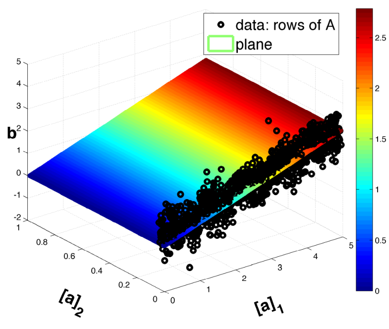
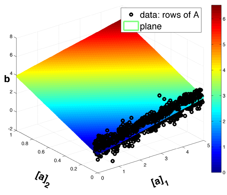
where is a matrix with ’s as its rows and is a vector with ’s as its components. The goal is to find a sparse vector (with many zero components) such that the error is minimized. To find one can solve problem (1). The purpose of the norm in (1) is to promote sparsity in the optimal solution [1]. An example that demonstrates the purpose of the norm is presented in Figure 1. Figure 1 shows a two dimensional instance where , and matrix is full-rank. Notice that the data points have large variations with respect to feature , where is the th component of the input vector, while there is only a small variation with respect to feature . This property is captured when problem (1) is solved with . The fitted plane in Figure 1a depends only on the first feature , while the second feature is ignored because , where is the optimal solution of (1). This can be observed through the level sets of the plane shown with the colored map; for each value of the level sets remain constant for all values of . On the contrary, this is not the case when one solves a simple least squares problem ( in (1)). Observe in Figure 1a that the fitted plane depends on both features and .
A variety of sparse data fitting applications originate from the fields of signal processing and statistics. Five representative examples are briefly described below.
- -
Magnetic Resonance Imaging (MRI): A medical imaging tool used to scan the anatomy and the physiology of a body [27].
- -
Image inpainting: A technique for reconstructing degraded parts of an image [7].
- -
Image deblurring: Image processing tool for removing the blurriness of a photo caused by natural phenomena, such as motion [21].
- -
Genome-Wide Association study (GWA): DNA comparison between two groups of people (with/without a disease) in order to investigate factors that a disease depends on [42].
- -
Estimation of global temperature based on historic data [22].
Data fitting problems frequently require the analysis of large scale data sets, i.e., gigabytes or terabytes of data. In order to address large scale problems there has been a resurgence in methods with computationally inexpensive iterations. For example many first-order methods were recovered and refined, such as coordinate descent [17, 24, 34, 39, 40, 41, 44, 45], alternating direction method of multipliers [9, 15, 18, 23, 43], proximal first-order methods [2, 12, 33] and first-order smoothing methods [5, 6, 30]. The previous are just few representative examples, the list is too long for a complete demonstration, many other examples can be found in [1, 11]. Often the goal of modern first-order methods is to reduce the computational complexity per iteration, while preserving the theoretical worst case iteration complexity of classic first-order methods [29]. Many modern first order methods meet the previous goal. For instance, coordinate descent methods can have up to times less computational complexity per iteration [35, 34].
First-order methods have been very successful in various scientific fields, such as support vector machine [46], compressed sensing [14], image processing [12] and data fitting [22]. Several new first-order type approaches have recently been proposed for various imaging problems in the special issue edited by M. Bertero, V. Ruggiero and L. Zanni [8]. However, even for the simple unconstrained problems that arise in the previous fields there exist more challenging instances. Since first-order methods do not capture sufficient second-order information, their performance might degrade unless the problems are well conditioned [16]. On the other hand, the second-order methods capture the curvature of the objective function sufficiently well, but by consensus they are usually applied only on medium scale problems or when high precision accuracy is required. In particular, it is frequently claimed [2, 5, 6, 20, 38] that the second-order methods do not scale favourably as the dimensions of the problem increase because of their high computational complexity per iteration. Such claims are based on an assumption that a full second-order information has to be used. However, there is evidence [16, 19] that for non-trivial problems, inexact second-order methods can be very efficient.
In this paper we will exhaustively study the performance of first- and second-order methods. We will perform numerical experiments for large-scale problems with sizes up to one trillion of variables. We will examine conditions under which certain methods are favoured or not. We hope that by the end of this paper the reader will have a clear view about the performance of first- and second-order methods.
Another contribution of the paper is the development of a rigorously defined instance generator for problems of the form of (1). The most important feature of the generator is that it scales well with the size of the problem and can inexpensively create instances where the user controls the sparsity and the conditioning of the problem. For example see Subsection 8.9, where an instance of one trillion variables is created using the proposed generator. We believe that the flexibility of the proposed generator will cover the need for generation of various good test problems.
This paper is organised as follows. In Section 2 we briefly discuss the structure of first- and second-order methods. In Section 3 we give the details of the instance generator. In Section 4 we provide examples for constructing matrix . In Section 5, we present some measures of the conditioning of problem (1). These measures will be used to examine the performance of the methods in the numerical experiments. In Section 6 we discuss how the optimal solution of the problem is selected. In Section 7 we briefly describe known problem generators and explain how our propositions add value to the existing approaches. In Section 8 we present the practical performance of first- and second-order methods as the conditioning and the size of the problems vary. Finally, in Section 9 we give our conclusions.
2 Brief discussion on first- and second-order methods
We are concerned with the performance of unconstrained optimization methods which have the following intuitive setting. At every iteration a convex function is created that locally approximates at a given point . Then, function is minimized to obtain the next point. An example that covers the previous setting is the Generic Algorithmic Framework (GFrame) which is given below. Details of GFrame for each method used in this paper are presented in Section 8.
| (3) |
Loosely speaking, close to the optimal solution of problem (1), the better the approximation of at any point the fewer iterations are required to solve (1). On the other hand, the practical performance of such methods is a trade-off between careful incorporation of the curvature of , i.e. second-order derivative information in and the cost of solving subproblem (3) in GFrame.
Discussion on two examples of which consider different trade-off follows. First, let us fix the structure of for problem (1) to be
| (4) |
where is a positive definite matrix. Notice that the decision of creating has been reduced to a decision of selecting . Ideally, matrix should be chosen such that it represents curvature information of at point , i.e. matrix should have similar spectral decomposition to . Let be a unit ball centered at . Then, should be selected in an optimal way:
| (5) |
The previous problem simply states that should minimize the sum of the absolute values of the residual over . Using twice the fundamental theorem of calculus on from to we have that (5) is equivalent to
| (6) |
It is trivial to see that the best possible is simply . However, this makes every subproblem (3) as difficult to be minimized as the original problem (1). One has to reevaluate the trade-off between a matrix that sufficiently well represents curvature information of at a point compared to a simple matrix that is not as good approximation but offers an inexpensive solution of subproblem (3). An example can be obtained by setting to be a positively scaled identity, which gives a solution to problem (5) , where denotes the largest eigenvalue of the input matrix and is the identity matrix of size . The contours of such a function compared to those of function are presented in Subfigure 2a. Notice that the curvature information of function is lost, this is because nearly all spectral properties of are lost.
However, for such a function the subproblem (3) has an inexpensive closed form solution known as iterative shrinkage-thresholding [12, 27]. The computational complexity per iteration is so low that one hopes that this will compensate for the losses of curvature information. Such methods, are called first-order methods and have been shown to be efficient for some large scale problems of the form of (1) [2].
Another approach of constructing involves the approximation of the -norm with the pseudo-Huber function
| (7) |
where is an approximation parameter. This approach is frequently used by methods that aim in using at every iteration full information from the Hessian matrix , see for example [16, 19]. Using (7), problem (1) is replaced with
| (8) |
The smaller is the better the approximation of problem (8) to (1). The advantage is that in (8) is a smooth function which has derivatives of all degrees. Hence, smoothing will allow access to second-order information and essential curvature information will be exploited. However, for very small certain problems arise for optimization methods of the form of GFrame, see [16]. For example, the optimal solution of (1) is expected to have many zero components, on the other hand, the optimal solution of (8) is expected to have many nearly zero components. However, for small one can expect to obtain a good approximation of the optimal solution of (1) by solving (8). For the smooth problem (8), the convex approximation at is:
| (9) |
The contours of such a function compared to function are presented in Subfigure 2b. Notice that captures the curvature information of function . However, minimizing the subproblem (3) might be a more expensive operation. Therefore, we rely on an approximate solution of (3) using some iterative method which requires only simple matrix-vector product operations with matrices and . In other words we use only an approximate second-order information. It is frequently claimed [2, 5, 6, 20, 38] that second-order methods do not scale favourably with the dimensions of the problem because of the more costly task of solving approximately the subproblems in (3), instead of having an inexpensive closed form solution. Such claims are based on an assumption that full second-order information has to be used when solving subproblem (3). Clearly, this is not necessary: an approximate second-order information suffices. Studies in [16, 19] provided theoretical background as well as the preliminary computational results to illustrate the issue. In this paper, we provide rich computational evidence which demonstrates that second-order methods can be very efficient.
3 Instance Generator
In this section we discuss an instance generator for (1) for the cases and . The generator is inspired by the one presented in Section of [32]. The advantage of our modified version is that it allows to control the properties of matrix and the optimal solution of (1). For example, the sparsity of matrix , its spectral decomposition, the sparsity and the norm of , since and are defined by the user.
Throughout the paper we will denote the component of a vector, by the name of the vector with subscript . Whilst, the column of a matrix is denoted by the name of the matrix with subscript .
3.1 Instance Generator for
Given , and the generator returns a vector such that . For simplicity we assume that the given matrix has rank . The generator is described in Procedure IGen below.
| (10) |
In procedure IGen, given , and we are aiming in finding a vector such that satisfies the optimality conditions of problem (1)
where is the subdifferential of the -norm at point . By fixing a subradient as defined in (10) and setting , the previous optimality conditions can be written as
| (11) |
The solution to the underdetermined system (11) is set to and then we simply obtain ; Steps and in IGen, respectively. Notice that for a general matrix , Step of IGen can be very expensive. Fortunately, using elementary linear transformations, such as Givens rotations, we can iteratively construct a sparse matrix with a known singular value decomposition and guarantee that the inversion of matrix in Step of IGen is trivial. We provide a more detailed argument in Section 4.
3.2 Instance Generator for
In this subsection we extend the instance generator that was proposed in Subsection 3.1 to the case of matrix with more columns than rows, i.e. . Given , , and the generator returns a vector and a matrix such that .
For this generator we need to discuss first some restrictions on matrix and the optimal solution . Let
| (12) |
with and be a collection of columns from matrix which correspond to indices in . Matrix must have rank otherwise problem (1) is not well-defined. To see this, let be the sign function applied component-wise to , where is a vector with components of that correspond to indices in . Then problem (1) reduces to the following:
| (13) |
where . The first-order stationary points of problem (13) satisfy
If , the previous linear system does not have a unique solution and problem (1) does not have a unique minimizer. Having this restriction in mind, let us now present the instance generator for in Procedure IGen2 below.
| (14) |
In IGen2, given , , and we are aiming in finding a vector and a matrix such that for , satisfies the optimality conditions of problem (1)
Without loss of generality it is assumed that all nonzero components of correspond to indices in . By fixing a partial subradient as in (14), where is a vector which consists of the first components of , and defining a vector , the previous optimality conditions can be written as:
| (15) |
It is easy to check that by defining as in Step of IGen2 conditions (15) are satisfied. Finally, we obtain .
Similarly to IGen in Subsection (3.1), for Step in IGen2 we have to perform a matrix inversion, which generally can be an expensive operation. However, in the next section we discuss techniques how this matrix inversion can be executed using a sequence of elementary orthogonal transformations.
4 Construction of matrix
In this subsection we provide a paradigm on how matrix can be inexpensively constructed such that its singular value decomposition is known and its sparsity is controlled. We examine the case of instance generator IGen where . The paradigm can be easily extended to the case of IGen2, where .
Let be a rectangular matrix with the singular values on its diagonal and zeros elsewhere:
where is a matrix of zeros, and let be a Givens rotation matrix, which rotates plane - by an angle :
where , and . Given a sequence of Givens rotations we define the following composition of them:
Similarly, let be a Givens rotation matrix where and
be a composition of Givens rotations. Using and we define matrix as
| (16) |
where are permutation matrices. Since the matrices and are orthonormal it is clear that the left singular vectors of matrix are the columns of , is the matrix of singular values and the right singular vectors are the columns of . Hence, in Step of IGen we simply set which means that Step in IGen costs two matrix-vector products with and a diagonal scaling with . Moreover, the sparsity of matrix is controlled by the numbers and of Givens rotations, the type, i.e. and , and the order of Givens rotations. Also, notice that the sparsity of matrix is controlled only by matrix . Examples are given in Subsection 4.1.
It is important to mention that other settings of matrix in (16) could be used, for example different combinations of permutation matrices and Givens rotations. The setting chosen in (16) is flexible, it allows for an inexpensive construction of matrix and makes the control of the singular value decomposition and the sparsity of matrices and easy.
Notice that matrix does not have to be calculated and stored. In particular, in case that the method which is applied to solve problem (1) requires only matrix-vector product operations using matrices and , one can simply consider matrix as an operator. It is only required to predefine the triplets for matrix , the triplets for matrix and the permutation matrices and . The previous implies that the generator is inexpensive in terms of memory requirements. Examples of matrix-vector product operations with matrices and in case of (16) are given below in Algorithms MvPA and MvPAt, respectively.
4.1 An example using Givens rotation
Let us assume that are divisible by two and . Given the singular values matrix and rotation angles and , we construct matrix as
where is a random permutation of the identity matrix, is a composition of Givens rotations:
with
and is a composition of Givens rotations:
with
Notice that the angle is the same for all Givens rotations , this means that the total memory requirement for matrix is low. In particular, it consists only of the storage of a rotation matrix. Similarly, the memory requirement for matrix is also low.
4.2 Control of sparsity of matrix and
We now present examples in which we demonstrate how sparsity of matrix can be controlled through Givens rotations.
In the example of Subsection 4.1, two compositions of and Givens rotations, denoted by G and , are applied on an initial diagonal rectangular matrix . If and the sparsity pattern of the resulting matrix is given in Subfigure 3a and has nonzero elements, while the sparsity pattern of matrix is given in Subfigure 4a and has nonzero elements. Notice in this subfigure that the coordinates can be clustered in pairs of coordinates , , and . One could apply another stage of Givens rotations. For example, one could construct matrix , where
with
and
with
Matrix has nonzeros and it is shown in Subfigure 3b, while matrix has nonzeros and it is shown in Subfigure 4b. By rotating again we obtain the matrix in Subfigure 3c with nonzero elements and matrix in Subfigure 4c with nonzero elements. Finally, the fourth Subfigures 3d and 4d show matrix and with and nonzero elements, respectively.
.
5 Conditioning of the problem
Let us now precisely define how we measure the conditioning of problem (1). For simplicity, throughout this section we assume that matrix has more rows than columns, , and it is full-rank. Extension to the case of matrix with more columns than rows is easy and we briefly discuss this at the end of this section.
We denote with the span of the columns of the input matrix. Moreover, is defined in (12), is its complement.
Two factors are considered that affect the conditioning of the problem. First, the usual condition number of the second-order derivative of in (1), which is simply , where are the eigenvalues of matrix . It is well-known that the larger is, the more difficult problem (1) becomes.
Second, the conditioning of the optimal solution of problem (1). Let us explain what we mean by the conditioning of . We define a constant and the index set . Furthermore, we define the projection , where , and matrix has as columns the eigenvectors of matrix which correspond to eigenvalues with indices in . Then, the conditioning of is defined as
| (17) |
For the case , the denominator of (17) is the mass of which exists in the space spanned by eigenvectors of which correspond to eigenvalues that are larger than or equal to .
Let us assume that there exists some which satisfies . If is large, i.e., is close to zero, then the majority of the mass of is “hidden” in the space spanned by eigenvectors which correspond to eigenvalues that are smaller than , i.e., the orthogonal space of . In Section 1 we referred to methods that do not incorporate information which correspond to small eigenvalues of . Therefore, if the previous scenario holds, then we expect the performance of such methods to degrade. In Section 8 we empirically verify the previous arguments.
If matrix has more columns than rows then the previous definitions of conditioning of problem (1) are incorrect and need to be adjusted. Indeed, if and , then is a rank deficient matrix which has nonzero eigenvalues and zero eigenvalues. However, we can restrict the conditioning of the problem to a neighbourhood of the optimal solution of . In particular, let us define a neighbourhood of so that all points in this neighbourhood have nonzeros at the same indices as and zeros elsewhere, i.e. . In this case an important feature to determine the conditioning of the problem is the ratio of the largest and the smallest nonzero eigenvalues of , where is a submatrix of built of columns of which belong to set .
6 Construction of the optimal solution
Two different techniques are employed to generate the optimal solution for the experiments presented in Section 8. The first procedure suggests a simple random generation of , see Procedure OsGen below.
The second and more complicated approach is given in Procedure OsGen2. This procedure is applicable only in the case that , however, it can be easily extended to the case of . We focus in the former scenario since all experiments in Section 8 are generated by setting .
The aim of Procedure OsGen2 is to find a sparse with arbitrarily large for some in the interval . In particular, OsGen2 will return a sparse which can be expressed as . The coefficients are close to the inverse of the eigenvalues of matrix . Intuitively, this technique will create an which has strong dependence on subspaces which correspond to small eigenvalues of . The constant is used in order to control the norm of .
The sparsity constraint in problem (18), i.e., , makes the approximate solution of this problem difficult when we use OMP, especially in the case that and are large. To avoid this expensive task we can ignore the sparsity constraint in (18). Then we can solve exactly and inexpensively the unconstrained problem and finally we can project the obtained solution in the feasible set defined by the sparsity constraint. Obviously, there is no guarantee that the projected solution is a good approximation to the one obtained in Step of Procedure OsGen2. However, for all experiments in Section 8 that we applied this modification we obtained sufficiently large . This means that our objective to produce ill-conditioned optimal solutions was met, while we kept the computational costs low. The modified version of Procedure OsGen2 is given in Procedure OsGen3.
| (19) |
7 Existing Problem Generators
So far in Section 3.1 we have described in details our proposed problem generator. Moreover, in Section 4 we have described how to construct matrices such that the proposed generator is scalable with respect to the number of unknown variables. We now briefly describe existing problem generators and explain how our propositions add value to the existing approaches.
Given a regularization parameter existing problem generators are looking for , and such that the optimality conditions of problem (1):
| (20) |
are satisfied. For example, in [32] the author fixes a vector of noise and an optimal solution and then finds and such that (20) is satisfied. In particular, in [32] matrix is used, where is a fixed matrix and is a scaling matrix such that the following holds.
Matrix is trivial to calculate, see Section in [32] for details. Then by setting (20) is satisfied. The advantage of this generator is that it allows control of the noise vector , in comparison to our approach where the vector noise has to be determined by solving a linear system. On the other hand, one does not have direct control over the singular value decomposition of matrix , since this depends on matrix , which is determined based on the fixed vectors and .
Another representative example is proposed in [26]. This generator, which we discovered during the revision of our paper, proposes the same setting as in our paper. In particular, given , and one can construct a vector (or a noise vector ) such that (20) is satisfied. However, in [26] the author suggests that can be found using a simple iterative procedure. Depending on matrix and how ill-conditioned it is, this procedure might be slow. In this paper, we suggest that one can rely on numerical linear algebra tools, such as Givens rotation, in order to inexpensively construct (or a noise vector ) using straightforwardly scalable operations. Additionally, we show in Section (8) that a simple construction of matrix is sufficient to extensively test the performance of methods.
8 Numerical Experiments
In this section we study the performance of state-of-the-art first- and second-order methods as the conditioning and the dimensions of the problem increase. The scripts that reproduce the experiments in this section as well as the problem generators that are described in Section 3 can be downloaded from: http://www.maths.ed.ac.uk/ERGO/trillion/.
8.1 State-of-the-art Methods
A number of efficient first- [2, 13, 24, 34, 35, 38, 39, 40, 41, 44, 45] and second-order [4, 10, 16, 19, 25, 36, 37] methods have been developed for the solution of problem (1). In this section we examine the performance of the following state-of-the-art methods. Notice that the first three methods FISTA, PSSgb and PCDM do not perform smoothing of the -norm, while pdNCG does.
- •
FISTA (Fast Iterative Shrinkage-Thresholding Algorithm) [2] is an optimal first-order method for problem (1), which adheres to the structure of GFrame. At a point , FISTA builds a convex function:
where is an upper bound of , and solves subproblem (3) exactly using shringkage-thresholding [12, 27]. An efficient implementation of this algorithm can be found as part of TFOCS (Templates for First-Order Conic Solvers) package [6] under the name N. In this implementation the parameter is calculated dynamically.
- •
PCDM (Parallel Coordinate Descent Method) [35] is a randomized parallel coordinate descent method. The parallel updates are performed asynchronously and the coordinates to be updated are chosen uniformly at random. Let be the number of processors that are employed by PCDM. Then, at a point , PCDM builds convex approximations:
, where is the th column of matrix and is the th diagonal element of matrix and is a positive constant which is defined in Subsection 8.3. The functions are minimized exactly using shrinkage-thresholding.
- •
PSSgb (Projected Scaled Subgradient, Gafni-Bertsekas variant) [37] is a second-order method. At each iteration of PSSgb the coordinates are separated into two sets, the working set and the active set . The working set consists of all coordinates for which, the current point is nonzero. The active set is the complement of the working set . The following local quadratic model is build at each iteration
where is a sub-gradient of at point with the minimum Euclidean norm, see Subsection 2.2.1 in [37] for details. Moreover, matrix is defined as:
where is an L-BFGS (Limited-memory Broyden-Fletcher-Goldfarb-Shanno) Hessian approximation with respect to the coordinates and is a positive diagonal matrix. The diagonal matrix is a scaled identity matrix, where the Shanno-Phua/Barzilai-Borwein scaling is used, see Subsection 2.3.1 in [37] for details. The local model is minimized exactly since the inverse of matrix is known due to properties of the L-BFGS Hessian approximation .
- •
pdNCG (primal-dual Newton Conjugate Gradients) [16] is also a second-order method. At every point pdNCG constructs a convex function exactly as described for (9). The subproblem (3) is solved inexactly by reducing it to the linear system:
which is solved approximately using preconditioned Conjugate Gradients (PCG). A simple diagonal preconditioner is used for all experiments. The preconditioner is the inverse of the diagonal of matrix .
8.2 Implementation details
Solvers pdNCG, FISTA and PSSgb are implemented in MATLAB, while solver PCDM is a C++ implementation. We expect that the programming language will not be an obstacle for pdNCG, FISTA and PSSgb. This is because these methods rely only on basic linear algebra operations, such as the dot product, which are implemented in ++ in MATLAB by default. The experiments in Subsections 8.4, 8.5, 8.6 were performed on a Dell PowerEdge R920 running Redhat Enterprise Linux with four Intel Xeon E7-4830 v2 2.2GHz processors, 20MB Cache, 7.2 GT/s QPI, Turbo (4x10Cores).
The huge scale experiments in Subsection 8.9 were performed on a Cray XC MPP supercomputer. This work made use of the resources provided by ARCHER (http://www.archer.ac.uk/), made available through the Edinburgh Compute and Data Facility (ECDF) (http://www.ecdf.ed.ac.uk/). According to the most recent list of commercial supercomputers, which is published in TOP list (http://www.top500.org), ARCHER is currently the fastest supercomputer worldwide out of supercomputers. ARCHER has a total of cores with performance TFlops/s on LINPACK benchmark and TFlops/s theoretical peak perfomance. The most computationally demanding experiments which are presented in Subsection 8.9 required more than half of the cores of ARCHER, i.e., cores out of .
8.3 Parameter tuning
We describe the most important parameters for each solver, any other parameters are set to their default values. For pdNCG we set the smoothing parameter to , this setting allows accurate solution of the original problem with an error of order [31]. For pdNCG, PCG is terminated when the relative residual is less that and the backtracking line-search is terminated if it exceeds iterations. Regarding FISTA the most important parameter is the calculation of the Lipschitz constant , which is handled dynamically by TFOCS. For PCDM the coordinate Lipschitz constants are calculated exactly and parameter , where changes for every problem since it is the degree of partial separability of the fidelity function in (1), which is easily calculated (see [35]), and is the number of cores that are used. For PSSgb we set the number of L-BFGS corrections to .
We set the regularization parameter , unless stated otherwise. We run pdNCG for sufficient time such that the problems are adequately solved. Then, the rest of the methods are terminated when the objective function in (1) is below the one obtained by pdNCG or when a predefined maximum number of iterations limit is reached. All comparisons are presented in figures which show the progress of the objective function against the wall clock time. This way the reader can compare the performance of the solvers for various levels of accuracy. We use logarithmic scales for the wall clock time and terminate runs which do not converge in about seconds, i.e., approximately hours.
8.4 Increasing condition number of
In this experiment we present the performance of FISTA, PCDM, PSSgb and pdNCG for increasing condition number of matrix when Procedure OsGen is used to construct the optimal solution . We generate six matrices and two instances of for every matrix ; twelve instances in total.
The singular value decomposition of matrix is , where is the matrix of singular values, the columns of matrices and are the left and right singular vectors, respectively, see Subsection 4.1 for details about the construction of matrix . The singular values of matrices are chosen uniformly at random in the intervals , where , for each of the six matrices . Then, all singular values are shifted by . The previous resulted in a condition number of matrix which varies from to with a step of times . The rotation angle of matrix is set to radians. Matrices have columns, rows and rank . The optimal solutions have nonzero components for all twelve instances.
For the first set of six instances we set in OsGen, which resulted in for all experiments. The results are presented in Figure 5. For these instances PCDM is clearly the fastest for , while for pdNCG is the most efficient.
For the second set of six instances we set in Procedure OsGen, which resulted in the same as before for every matrix . The results are presented in Figure 6. For these instances PCDM is the fastest for very well conditioned problems with , while pdNCG is the fastest for .
We observed that pdNCG required at most 30 iterations to converge for all experiments. For FISTA, PCDM and PSSgb the number of iterations was varying between thousands and tens of thousands iterations depending on the condition number of matrix ; the larger the condition number the more the iterations. However, the number of iterations is not a fair metric to compare solvers because every solver has different computational cost per iteration. In particular, FISTA, PCDM and PSSgb perform few inner products per iteration, which makes every iteration inexpensive, but the number of iterations is sensitive to the condition number of matrix . On the other hand, for pdNCG the empirical iteration complexity is fairly stable, however, the number of inner products per iteration (mainly matrix-vector products with matrix ) may increase as the condition number of matrix increases. Inner products are the major computational burden at every iteration for all solvers, therefore, the faster an algorithm converged in terms of wall-clock time the less inner products that are calculated. In Figures 5 and 6 we display the objective evaluation against wall-clock time (log-scale) to facilitate the comparison of different algorithms.
8.5 Increasing condition number of : non-trivial construction of
In this experiment we examine the performance of the methods as the condition number of matrix increases, while the optimal solution is generated using Procedure OsGen3 (instead of OsGen) with and . Two classes of instances are generated, each class consists of four instances with , and . Matrix is constructed as in Subsection 8.4. The singular values of matrices are chosen uniformly at random in the intervals , where , for all generated matrices . Then, all singular values are shifted by . The previous resulted in a condition number of matrix which varies from to with a step of times . The condition number of the generated optimal solutions was on average .
The two classes of experiments are distinguished based on the rotation angle that is used for the composition of Givens rotations . In particular, for the first class of experiments the angle is radians, while for the second class of experiments the rotation angle is radians. The difference between the two classes is that the second class consists of matrices for which, a major part of their mass is concentrated in the diagonal. This setting is beneficial for PCDM since it uses information only from the diagonal of matrices . This setting is also beneficial for pdNCG since it uses a diagonal preconditioner for the inexact solution of linear systems at every iteration.
The results for the first class of experiments are presented in Figure 7. For instances with PCDM was terminated after iterations, which corresponded to more than hours of wall-clock time.
The results for the second class of experiments are presented in Figure 8. Notice in this figure that the objective function is only slightly reduced. This does not mean that the initial solution, which was the zero vector, was nearly optimal. This is because noise with large norm, i.e., is large, was used in these experiments, therefore, changes in the optimal solution did not have large affect on the objective function.
8.6 Increasing dimensions
In this experiment we present the performance of pdNCG, FISTA, PCDM and PSSgb as the number of variables increases. We generate four instances where the number of variables takes values , , and , respectively. The singular value decomposition of matrix is . The singular values in matrix are chosen uniformly at random in the interval and then are shifted by , which resulted in . The rotation angle of matrix is set to radians. Moreover, matrices have rows and rank . The optimal solutions have nonzero components for each generated instance. For the construction of the optimal solutions we use Procedure OsGen3 with and , which resulted in on average.
The results of this experiment are presented in Figure 9. Notice that all methods have a linear-like scaling with respect to the size of the problem.
8.7 Increasing density of matrix
In this experiment we demonstrate the performance of pdNCG, FISTA, PCDM and PSSgb as the density of matrix increases. We generate four instances . For the first experiment we generate matrix , where is the matrix of singular values, the columns of matrices and are the left and right singular vectors, respectively. For the second experiment we generate matrix , where the columns of matrices and are the left and right singular vectors of matrix , respectively; has been defined in Subsection 4.2. Finally, for the third and fourth experiments we have and , respectively. For each experiment the singular values of matrix are chosen uniformly at random in the interval and then are shifted by , which resulted in . The rotation angle of matrices and is set to radians. Matrices have rows, rank and . The optimal solutions have nonzero components for each experiment. Moreover, Procedure OsGen3 is used with and for the construction of for each experiment, which resulted in on average.
The results of this experiment are presented in Figure 10. Observe, that all methods had a robust performance with respect to the density of matrix .
8.8 Varying parameter
In this experiment we present the performance of pdNCG, FISTA, PCDM and PSSgb as parameter varies from to with a step of times . We generate four instances , where matrix has rows, rank and . The singular values of matrices are chosen uniformly at random in the interval and then are shifted by , which resulted in for each experiment. The rotation angles for matrix in is set to radians. The optimal solution has nonzero components for all instances. Moreover, the optimal solutions are generated using Procedure OsGen3 with , which resulted in for all four instances.
The performance of the methods is presented in Figure 11. Notice in Subfigure 11d that for pdNCG the objective function is not always decreasing monotonically. A possible explanation is that the backtracking line-search of pdNCG, which guarantees monotonic decrease of the objective function [16], terminates in case that backtracking iterations are exceeded, regardless if certain termination criteria are satisfied.
8.9 Performance of a second-order method on huge scale problems
We now present the performance of pdNCG on synthetic huge scale (up to one trillion variables) S-LS problems as the number of variables and the number of processors increase.
We generate six instances , where the number of variables takes values , , , , and . Matrices have rows and rank . The singular values for of matrices are set to for odd ’s and for even ’s. The rotation angle of matrix is set to radians. The optimal solutions have nonzero components for each experiment. In order to simplify the practical generation of this problem the optimal solutions are set to have components equal to and the rest of nonzero components are set equal to .
Details of the performance of pdNCG are given in Table 1. Observe the nearly linear scaling of pdNCG with respect to the number of variables and the number of processors. For all experiments in Table 1 pdNCG required Newton steps to converge, PCG iterations per Newton step on average, where every PCG iteration requires two matrix-vector products with matrix .
| Processors | Memory (terabytes) | Time (seconds) | |
|---|---|---|---|
| 1,923 | |||
| 1,968 | |||
| 1,986 | |||
| 1,970 | |||
| 1,990 | |||
| 2,006 |
9 Conclusion
In this paper we developed an instance generator for -regularized sparse least-squares problems. The generator is aimed for the construction of very large-scale instances. Therefore it scales well as the number of variables increases, both in terms of memory requirements and time. Additionally, the generator allows control of the conditioning and the sparsity of the problem. Examples are provided on how to exploit the previous advantages of the proposed generator. We believe that the optimization community needs such a generator to be able to perform fair assessment of new algorithms.
Using the proposed generator we constructed very large-scale sparse instances (up to one trillion variables), which vary from very well-conditioned to moderately ill-conditioned. We examined the performance of several representative first- and second-order optimization methods. The experiments revealed that regardless of the size of the problem, the performance of the methods crucially depends on the conditioning of the problem. In particular, the first-order methods PCDM and FISTA are faster for problems with small or moderate condition number, whilst, the second-order method pdNCG is much more efficient for ill-conditioned problems.
Acknowledgements.
This work has made use of the resources provided by ARCHER (http://www.archer.ac.uk/), made available through the Edinburgh Compute and Data Facility (ECDF) (http://www.ecdf.ed.ac.uk/). The authors are grateful to Dr Kenton D’ Mellow for providing guidance and helpful suggestions regarding the use of ARCHER and the solution of large scale problems.References
- [1] F. Bach, R. Jenatton, J. Mairal, and G. Obozinski. Optimization with sparsity-inducing penalties. Journal Foundations and Trends in Machine Learning, 4(1):1–106, 2012.
- [2] A. Beck and M. Teboulle. A fast iterative shrinkage-thresholding algorithm for linear inverse problems. SIAM J. Imaging Sci., 2(1):183–202, 2009.
- [3] S. Becker. CoSaMP and OMP for sparse recovery. http://www.mathworks.co.uk/matlabcentral/fileexchange/32402-cosamp-and-omp-for-sparse-recovery, 2012.
- [4] S. Becker and J. Fadili. A quasi-Newton proximal splitting method. In F. Pereira, C.J.C. Burges, L. Bottou, and K.Q. Weinberger, editors, Advances in Neural Information Processing Systems 25, pages 2618–2626. Curran Associates, Inc., 2012.
- [5] S. R. Becker, J. Bobin, and E. J. Candès. Nesta: A fast and accurate first-order method for sparse recovery. SIAM J. Imaging Sciences, 4(1):1–39, 2011.
- [6] S. R. Becker, E. J. Candés, and M. C. Grant. Templates for convex cone problems with applications to sparse signal recovery. Mathematical Programming Computation, 3(3):165–218, 2011. Software available at http://tfocs.stanford.edu.
- [7] M. Bertalmio, G. Sapiro, C. Ballester, and V. Caselles. Image inpainting. Proceedings of the 27th annual conference on Computer graphics and interactive techniques (SIGGRAPH), pages 417–424, 2000.
- [8] M. Bertero, V. Ruggiero, and L. Zanni. Special issue: Imaging 2013. Computational Optimization and Applications, 54:211–213, 2013.
- [9] S. Boyd, N. Parikh, E. Chu, B. Peleato, and J. Eckstein. Distributed optimization and statistical learning via the alternating direction method of multipliers. Journal Foundations and Trends in Machine Learning, 3(1):1–122, 2011.
- [10] R. H. Byrd, J. Nocedal, and F. Oztoprak. An inexact successive quadratic approximation method for convex l-1 regularized optimization. Math. Program., Ser. B, 2015. DOI: 10.1007/s10107-015-0941-y.
- [11] A. Chambolle, V. Caselles, D. Cremers, M. Novaga, and T. Pock. An introduction to total variation for image analysis. Radon Series Comp. Appl. Math, 9:263–340, 2010.
- [12] A. Chambolle, R. A. DeVore, N. Y. Lee, and B. J. Lucier. Nonlinear wavelet image processing: Variational problems, compression, and noise removal through wavelet shrinkage. IEEE Trans. Image Process., 7(3):319–335, 1998.
- [13] K.-W. Chang, C.-J. Hsieh, and C.-J. Lin. Coordinate descent method for large-scale -loss linear support vector machines. Journal of Machine Learning Research, 9:1369–1398, 2008.
- [14] D. L. Donoho. Compressed sensing. IEEE Trans. Inf. Theory, 52(4):1289–1306, 2006.
- [15] J. Eckstein. Augmented lagrangian and alternating direction methods for convex optimization: A tutorial and some illustrative computational results. RUTCOR Research Reports, 2012.
- [16] K. Fountoulakis and J. Gondzio. A second-order method for strongly convex -regularization problems. Mathematical Programming (accepted), 2015. DOI: 10.1007/s10107-015-0875-4, Software available at http://www.maths.ed.ac.uk/ERGO/pdNCG/.
- [17] J. Friedman, T. Hastie, and R. Tibshirani. Regularization paths for generalized linear models via coordinate descent. Journal of Machine Learning Research, 9:627–650, 2008.
- [18] T. Goldstein, B. O’Donoghue, and S. Setzer. Fast alternating direction optimization methods. Technical report, CAM Report 12-35, UCLA, 2012.
- [19] J. Gondzio. Matrix-free interior point method. Computational Optimization and Applications, 51(2):457–480, 2012.
- [20] E. T. Hale, W. Yin, and Y. Zhang. Fixed-point continuation method for -minimization: Methodology and convergence. SIAM J. Optim., 19(3):1107–1130, 2008.
- [21] P. C. Hansen, J. G. Nagy, and D. P. O’Leary. Deblurring Images: Matrices, Spectra and Filtering. SIAM, Philadelphia, PA., 2006.
- [22] P. C. Hansen, V. Pereyra, and G. Scherer. Least Squares Data Fitting with Applications. JHU Press, 2012.
- [23] B. He and X. Yuan. On the convergence rate of alternating direction method. SIAM Journal on Numerical Analysis, 50(2):700–709, 2012.
- [24] C.-J. Hsieh, K.-W. Chang, C.-J. Lin, S. S. Keerthi, and S. Sundararajan. A dual coordinate descent method for large-scale linear SVM. Proceedings of the 25th international conference on Machine Learning, ICML 2008, pages 408–415, 2008.
- [25] S.-J. Kim, K. Koh, M. Lustig, S. Boyd, and D. Gorinevsky. An interior-point method for large-scale -regularized least squares. IEEE Journal Of Selected Topics In Signal Processing, 1(4):606–617, 2007.
- [26] D. A. Lorenz. Constructing test instances for basis pursuit denoising. IEEE Trans. Signal Process., 61(5):1210–1214, 2013.
- [27] M. Lustig, D. Donoho, and J. M. Pauly. Sparse MRI: The application of compressed sensing for rapid MR imaging. Magnetic Resonance in Medicine, 58(6):1182–1195, 2007.
- [28] D. Needell and J. A. Tropp. Cosamp: Iterative signal recovery from incomplete and inaccurate samples. Applied and Computational Harmonic Analysis, 26(3):301–321, 2009.
- [29] Y. Nesterov. Introductory Lecture Notes On Convex Optimization. A Basic Course. Kluver, Boston, 2004.
- [30] Y. Nesterov. Smooth minimization of non-smooth functions. Mathematical Programming, 103(1):127–152, 2005.
- [31] Y. Nesterov. Smooth minimization of non-smooth functions. Math. Program., 103(1):127–152, 2005.
- [32] Yu. Nesterov. Gradient methods for minimizing composite functions. Mathematical Programming, 140(1):125–161, 2013.
- [33] N. Parikh and S. Boyd. Proximal algorithms. Journal Foundations and Trends in Optimization, 1(3):123–231, 2013.
- [34] P. Richtárik and M. Takáč. Iteration complexity of randomized block-coordinate descent methods for minimizing a composite function. Math. Program. Ser. A, 144(1):1–38, 2014.
- [35] P. Richtárik and M. Takáč. Parallel coordinate descent methods for big data optimization. Math. Program. Ser. A, pages 1–52, 2015. DOI: 10.1007/s10107-015-0901-6.
- [36] K. Scheinberg and X. Tang. Practical inexact proximal quasi-Newton method with global complexity analysis. Technical report, March 2014. arXiv:1311.6547 [cs.LG].
- [37] M. Schmidt. Graphical model structure learning with l1-regularization. PhD thesis, University British Columbia, 2010.
- [38] S. Shalev-Shwartz and A. Tewari. Stochastic methods for -regularized loss minimization. Journal of Machine Learning Research, 12(4):1865–1892, 2011.
- [39] P. Tseng. Convergence of a block coordinate descent method for nondifferentiable minimization. Journal of Optimization Theory and Applications, 109(3):475–494, 2001.
- [40] P. Tseng. Efficiency of coordinate descent methods on huge-scale optimization problems. SIAM J. Optim., 22:341–362, 2012.
- [41] P. Tseng and S. Yun. A coordinate gradient descent method for nonsmooth separable minimization. Math. Program., Ser. B, 117:387–423, 2009.
- [42] S. Vattikuti, J. J. Lee, C. C. Chang, S. D. Hsu, and C. C. Chow. Applying compressed sensing to genome-wide association studies. GigaScience, 3(10):1–17, 2014.
- [43] Y. Wang, J. Yang, W. Yin, and Y. Zhang. A new alternating minimization algorithm for total variation image reconstruction. SIAM Journal on Imaging Sciences, 1(3):248–272, 2008.
- [44] S. J. Wright. Accelerated block-coordinate relaxation for regularized optimization. SIAM Journal on Optimization, 22(1):159–186, 2012.
- [45] T. T. Wu and K. Lange. Coordinate descent algorithms for lasso penalized regression. The Annals of Applied Statistics, 2(1):224–244, 2008.
- [46] G.-X. Yuan, K.-W. Chang, C.-J. Hsieh, and C.-J. Lin. A comparison of optimization methods and software for large-scale -regularized linear classification. Journal of Machine Learning Research, 11:3183–3234, 2010.