Experimental level densities of atomic nuclei
Abstract
It is almost 80 years since Hans Bethe described the level density as a non-interacting gas of protons and neutrons. In all these years, experimental data were interpreted within this picture of a fermionic gas. However, the renewed interest of measuring level density using various techniques calls for a revision of this description. In particular, the wealth of nuclear level densities measured with the Oslo method favors the constant-temperature level density over the Fermi-gas picture. From the basis of experimental data, we demonstrate that nuclei exhibit a constant-temperature level density behavior for all mass regions and at least up to the neutron threshold.
pacs
PACS-key21.10.Ma, 25.20.Lj, 25.40.Hs1 Introduction
The level density of atomic nuclei provides important information on the heated nucleonic many-particle system. In the pioneering work of Hans Bethe in 1936 [1], the level density was described as a gas of non-interacting fermions moving in equally spaced single-particle orbitals. Despite the scarce nuclear structure knowledge at that time, this Fermi-gas model contained the essential components apart from the influence of the pairing force between nucleons in time-reversed orbitals. The understanding of such Cooper pairs and the nuclear structure consequences, was first realized twenty years later through the Bardeen-Cooper-Schrieffer (BCS) theory [2].
Unfortunately, the new knowledge of the pairing force was implemented in an oversimplified way by still assuming a gas of fermions. The original Fermi-gas level density curve was simply shifted up in energy by and for the description of odd-mass and even-even mass nuclei, respectively. Later, this energy correction was found to be too large, and the shift was somewhat back-shifted again. The resulting back-shifted Fermi-gas model has since then been very popular and has been the most common description of nuclear level densities for decades [3]. These manipulations maintained the typical Fermi-gas level density shape with excitation energy .
There is a growing interest in the nuclear science community for the study of nuclear level densities. The introduction of novel theoretical approaches and fast computers has opened the way for a microscopical description of heavier nuclei up to high excitation energy [4]. Thus, experimental level densities represent a basic testing ground for many-particle nuclear structure models. They also have an increasing importance for various nuclear applications. Nuclear level densities play an essential role in the calculation of reaction cross sections applied to astrophysical nucleosynthesis, nuclear energy production and transmutation of nuclear waste.
The number of levels is exponentially increasing with excitation energy and typically for the rare earth region, the level density increases by a factor of one million when going from the ground state up to the neutron binding energy. This tremendous change has implications for the theoretical interpretations since levels start to overlap in energy at high excitation energies, typically around 10-15 MeV. Thus, nuclear excitations are often divided into three regimes [5], classified by the average level spacings compared to the -decay width . These key numbers are connected to the level density and life time by and , respectively. Figure 1 illustrates the connections between the three regimes i.e. the discrete, quasi-continuum and continuum regions.
Experimentally, the quasi-continuum region is often defined as the region where the experimental resolution prevents the separation into individual levels. This appears when . One should be aware that this definition depends on the selectivity of the reactions used and the specific experimental detectors and conditions. In this work, the experimental quasi-continuum region starts when keV, i.e. when the level density exceeds MeV-1.

Today various experimental techniques are used to determine nuclear level densities. The obvious method in the discrete region of Fig. 1 is to count the number of levels per excitation energy bin , readily giving the level density as . This requires that all levels are known. Making a short review on known discrete levels, e.g. in the compilation of Ref. [6], we find that the data set starts to be incomplete where the first Cooper pairs are broken, i.e. at excitation energies . This is simply because the high density of levels makes conventional spectroscopy difficult. A rule of thumb is that when MeV-1, the number of missing levels is dramatically increasing.
Level density information at the neutron separation energy can be extracted from neutron capture resonance spacings [7]. The spin selection of these resonances depends on the target ground-state spin and the neutron spin transfer, giving level densities for a narrow spin window, only. In particular, thermal neutrons with angular momentum transfer results in a spin window of . At higher excitation energies the method of Ericson fluctuations can be used [5]. A well known technique [8] is to extract the level density from particle evaporation spectra. The measurement must be carried out at backwards center-of-mass angles to avoid direct reaction contributions. The method also requires well determined optical potential model parameters. Furthermore, the level density can be extracted in the two-step cascade method [9] from simulations provided that the -ray strength function is known. An upcoming technique, see e.g. Ref. [10], is to use high-energy light-ion reactions like , and He, at small angles with respect to the beam direction. These reactions select the population of discrete levels with certain spin/parity assignments, information that is essential in the detailed understanding of level densities. This method requires that the spacings of the selected levels are larger or comparable to the experimental particle resolution.
In the present work we will show level densities of several nuclei measured at the Oslo Cyclotron Laboratory (OCL). The technique used, the Oslo method [11, 12], is unique in the sense that it allows for a simultaneous determination of the level density and the -ray strength function without assuming any models for these functions.
The structure of the manuscript is as follows: Section 2 describes briefly the experimental set-up and the Oslo method, and previously measured level densities will be discussed in Sect. 3. Finally, concluding remarks and outlooks are presented in Sect. 4.
2 The Oslo Method
The Oslo method is based on a set of spectra as a function of excitation energy. The excitation of the nucleus is performed by light ion reactions, e.g. , and He, where the energy of the charged ejectile determines the excitation energy.
A schematic drawing of the set-up is shown in Fig. 2. A silicon particle detection system (SiRi) [13], which consists of 64 telescopes, is used for the selection of a certain ejectile type and to determine its energies. The front and back detectors have thicknesses of 130 m and 1550 m, respectively. SiRi is usually placed in backward angles covering to relative to the beam axis. Coincidences with rays are performed with the CACTUS array [14], consisting of 26 collimated NaI(Tl) detectors with a total efficiency of % at MeV.

Figure 3 demonstrates the previously measured
237NpNp reaction [15] and
how one can proceed from the raw particle- coincidences to the first generation or primary -ray spectra. The first step
is to sort the events into a raw particle- matrix with proper subtraction of
random coincidences. Then, for all initial excitation energies , the spectra are unfolded with the NaI response
functions giving the matrix [16]. The procedure is iterative and stops
when the folding of the unfolded matrix equals the raw matrix within the statistical fluctuations, i.e. when
.

The primary -ray spectra can be extracted from the unfolded total spectra of Fig. 3 (b). The primary spectrum at an initial excitation energy is obtained by subtracting a weighted sum of spectra below excitation energy :
| (1) |
The weighting coefficients are determined in an iterative way described in Ref. [18]. After a few iterations, converges to , where we have normalized each spectrum by . This equality is exactly what is expected, namely that the primary -ray spectrum equals to the weighting function. The validity of the procedure rests on the assumption that the -energy distribution is the same whether the levels were populated directly by the nuclear reaction or by decay from higher-lying states. This is illustrated in Fig. 4.
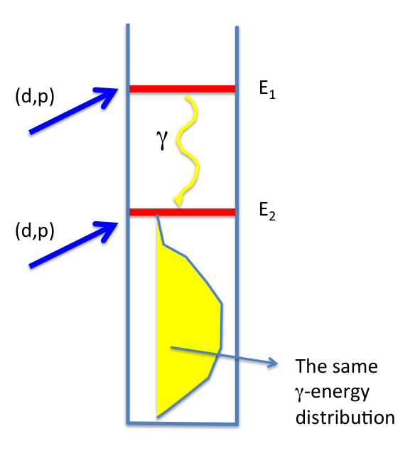
The statistical part of this landscape of probability, , is then assumed to be described by the product of two vectors
| (2) |
where the decay probability should be proportional to the level density at the final energy according to Fermi’s golden rule [19, 20]. The decay is also proportional to the -ray transmission coefficient , which according to the Brink hypothesis [21], is independent of excitation energy; only the transitional energy plays a role.
The values of the vector elements of and are varied freely to obtain a least- fit to the experimental matrix. Figure 5 shows that the product of of Eq. (2) fits very well the primary spectra of 238Np at the six excitation energy bins shown. There are actually four times more spectra and the same quality of fit is obtained for all spectra.
However, the nice fit to the data does not mean that and are uniquely determined. There are infinitely many functions that make identical fits to the experimental matrix. These and functions can be generated by the transformations [11]
| (3) | |||||
| (4) |
Thus, the normalization of the two functions requires information to fix the parameters , , and , which is not available from our experiment.
For the level density, we use two anchor points to determine and . The procedure is demonstrated for the case of 238Np in Fig. 6. The level density is normalized to known discrete levels at low excitation energy. At high excitation energy, we exploit the neutron resonance spacings at the neutron separation energy . In order to translate the spacing to level density, we use the spin distribution [17]
| (5) |
where is excitation energy and is spin. Here, the spin cut-off parameter is rather uncertain, and may introduce an uncertainty of a factor of 2 in . For cases where is unknown, one has to use systematics to estimate . Since the strength is not discussed in this work, the determination of the parameter is irrelevant. Further description and tests of the Oslo method are given in Refs. [11, 12].
3 Experimental level densities
| Reaction | Refs. | ||||
|---|---|---|---|---|---|
| (MeV) | (MeV) | (MeV) | (MeV-1) | ||
| Ti | 9.530 | 1.55 | -2.33 | 0.0014(7) | [22] |
| Ti | 13.189 | 1.70 | -2.07 | 0.0047(10) | [23] |
| Y | 11.478 | 1.00 | 0.48 | 0.060(20) | [24] |
| Y | 6.857 | 1.00 | -1.38 | 0.0038(8) | [24] |
| (3He,Sn | 9.563 | 0.76 | -0.03 | 0.40(20) | [25, 26, 27, 28] |
| (3He,3He′)117Sn | 6.944 | 0.67 | -0.40 | 0.091(27) | [25, 26, 27, 28] |
| (3He,)163Dy | 6.271 | 0.59 | -1.55 | 0.96(12) | [29] |
| (3He,3He′)164Dy | 7.658 | 0.60 | -0.66 | 1.74(21) | [29] |
| (Np | 5.488 | 0.41 | -1.35 | 43.0(78) | [15] |
The Oslo group has now published more than 70 level densities. Some of these are for one and the same nucleus, but populated with different reactions. The full compilation of level densities (and -ray strength functions) is found in Ref. [30]. We will here focus on some selected nuclei in order to convey to the reader a general picture of how the level density behaves as function of mass region and excitation energy. The references and key numbers are given in Table 1.
There is a tremendous span in level densities when going from mass around to 240. Figure 7 shows that the level density at excitation energy MeV for 238Np is almost ten million times higher than for 46Ti. It seems obvious that more nucleons produce higher level density, but this conclusion is not strictly true.
Indeed, we see that the level density for 90Y is larger than for 89Y. Also 117Sn has more levels than 116Sn. However, 45Ti has more levels than 46Ti and the same is true for 163Dy versus 164Dy. The pieces fall into place if pairing is taken into account: For neighboring isotopes, the nucleus with either one or more unpaired protons or neutrons displays times more levels. An increase in only gives negligible effects between neighboring nuclei, as e.g. found for the even-even 160,162,164Dy isotopes [31].
The number of quasi-particles is the basis building blocks for the level density. However, the number of active particles making the level density is not that different for 238Np and 46Ti. The odd-odd 238Np has about 6 quasi-particles at MeV, while 46Ti has about 2 quasi-particles. The second factor needed to understand the general behaviour of the level density is the density of available single-particle orbitals in the vicinity of the Fermi level where the quasi-particles can play around. In summary, the large span in level density between and 240 is a combined result of the number of quasi-particles and the density of near lying single-particle orbitals.
Another striking feature of Fig. 7 is that, above a certain excitation energy , the level densities are linear in a log-plot, which corresponds to an exponential function. The 45Ti has an exponential behavior for MeV, whereas 238Np has it for MeV. Generally, the exponential behavior sets in when the first nucleon pairs are broken, i.e. . With a pairing gap of MeV, we find for the two cases and MeV, respectively. The level density is not only dependent on the atomic mass number , but also on the number of unpaired nucleons around the ground state. As an example, the exponential behavior is delayed for even-even nuclei compared to odd-even nuclei. This is e.g. apparent for 116,117Sn and 163,164Dy.
The interpretation of the pure exponential growth above has recently been discussed in Ref. [31]. For the micro-canonical ensemble, the entropy is related to the level density by
| (6) |
with
| (7) |
Thus, the temperature is constant when is linear in . The common expression for the constant-temperature level density is [5]
| (8) |
where is determined by the slope of . This is the key characteristic of a first-order phase transition. Our interpretation of the data is that the energy goes into breaking Cooper pairs and thus the temperature remains constant. The obvious analogy is the melting of ice to water at constant temperature. The fit parameters and for the nuclei shown in Fig. 7 are listed in Table 1.
Figure 8 shows that the constant-temperature level density model fits the data of 164Dy much better than the Fermi gas model. The reduced fit value evaluated between excitation energies and MeV is about a factor of 10 better for the CT model. One should of course mention that the CT model is not a perfect model. There are some oscillations in the experimental log-plot mainly due to the onset of the two and four quasi-particle regimes.
Recommendations are available for the Fermi-gas spin-cut off parameter [32]. However, for the CT-model there are no clear recommendations. According to the original expression of Ericson [5]:
| (9) |
we see that for the CT model, only the moment of inertia will depend on , since is a constant. There are indications [33] that the rigid moment of inertia is reached at the neutron separation energy, i.e. . However, how to parameterize to lower excitation energies is still uncertain. In addition to the uncertain spin distribution, the parity distribution is important for lighter nuclei and nuclei close to magic numbers. There are only few experimental data available in order to pin down the spin and parity distributions and this represents perhaps the most important issue for future research on nuclear level densities.
The pair breaking process will continue at least up to the binding energy, but probably to much higher excitations. In several evaporation experiments the constant temperature behavior has been observed up to MeV [34, 35]. However, at the higher excitation energies the temperature will start increasing with excitation energies, and the Fermi gas description [1, 3] will to an increasing degree describe the data.
4 Concluding remarks and outlook
The present work describes the Oslo method and results using light-ion reactions on stable targets. The method is demonstrated by means of the 237NpNp reaction, which provides almost ideal conditions for the Oslo method. One important aim of these investigations is to obtain more predictive power for extrapolation of the level densities to nuclei outside the valley of -stability.
From light (45Ti) to the heavy elements (238Np) we find certain common features of the level densities. It turns out that the pairing force is responsible for the mechanism behind these features. The level density above the excitation energy of 2 behaves as an exponential curve characterized by the nuclear temperature. Furthermore, neighboring nuclei have the same temperature and their respective level densities appear parallel in a log plot. Odd-mass nuclei exhibit about times more levels than their even-even partners. There are indications that each unpaired nucleon carry approximately an entropy of , corresponding to the multiplicative factor above.
In the field of experimental level densities, there are several skeletons in the closet. In particular, it is crucial to get more information on the true spin and parity distributions as function of excitation energy and mass. The few experimental data on these quantities also have implications for applications when e.g. calculating reaction rates. Today, such information is often taken from theoretical models without verifications based on experimental observations.
In the energy regime from the ground state up to the energy where the breaking of the first Cooper pairs set in, the level density depends strongly on the specific nuclear structure properties of the nucleus studied. For even-even nuclei, the level density is determined by the collective modes like rotation and vibrations. For the odd-mass nuclei the unpaired valence nucleon already carries a quasi-particle entropy that adds to these collective degrees of freedom.
A great challence is to obtain data also for nuclei far away from the -stability line, nuclei that are essential for nucleo-synthesis networks and other applications. Since it is a rather uncertain approach to extrapolate results from more stable nuclei to these nuclei, novel experimental techniques are needed. The Oslo group has already initiated experiments to measure level densities for short-lived nuclei. The so-called -Oslo method is based on the population of rare nuclei by means of decay. The first experiment, which was performed at the National Superconducting Cyclotron Laboratory at Michigan State University (MSU) using the SuN detector has already been published [36], and several new experiments have been carried out. Also inverse kinematic experiments with radioactive beams are planned at HIE-ISOLDE.
The constant-temperature level density behavior is expected also for nuclei far from the -stability line. However, when the particle separation energies approaches the paring energy of , the individual low-lying discrete levels will play an increasing role. Furthest away from the valley of stability, discrete spectroscopy of low-lying levels will probably be the way to proceed. In such scenarios the concept of level density will lose its importance and be replaced by discrete spectroscopy.
References
- (1) H.A. Bethe, Phys. Rev. 50, 332 (1936).
- (2) J. Bardeen, L.N. Cooper, and J.R. Schrieffer, Phys. Rev. 108, 1175 (1957).
- (3) R. Capote et al., Nucl. Data Sheets 110 (2009) 3107.
- (4) S. Goriely, N. Chamel and J.M. Pearson, Phys. Rev. Lett. 102, 152503 (2009).
- (5) T. Ericson, Nucl. Phys. A 11, 481 (1959).
- (6) Data from the NNDC On-Line Data Service database; available at http://www.nndc.bnl.gov/nudat2/.
- (7) RIPL-3 Handbook for calculation of nuclear reaction, (2009); available at http://www-nds.iaea.org/RIPL-3/.
- (8) H. K. Vonach and J. R. Huizenga, Phys. Rev. 149, 844 (1966).
- (9) A.M. Hoogenboom, Nucl. Instrum. Methods 3, 57 (1958).
- (10) Y. Kalmykov, C. Özen, K. Langanke, G. Martínez-Pinedo, P. von Neumann-Cosel and A. Richter, Phys. Rev. Lett. 99, 202502 (2007)
- (11) A. Schiller, L. Bergholt, M. Guttormsen, E. Melby, J. Rekstad, and S. Siem, Nucl. Instrum. Methods Phys. Res. A 447 494 (2000).
- (12) A.C. Larsen et al., Phys. Rev. C 83, 034315 (2011).
- (13) M. Guttormsen, A. Bürger, T.E. Hansen, and N. Lietaer, Nucl. Instrum. Methods Phys. Res. A 648, 168 (2011).
- (14) M. Guttormsen, A. Atac, G. Løvhøiden, S. Messelt, T. Ramsøy, J. Rekstad, T.F. Thorsteinsen, T.S. Tveter, and Z. Zelazny, Phys. Scr. T 32, 54 (1990).
- (15) T. G. Tornyi, M. Guttormsen, T. K. Eriksen, A. Görgen, F. Giacoppo, T. W. Hagen, A. Krasznahorkay, A. C. Larsen, T. Renstrøm, S. J. Rose, S. Siem, and G. M. Tveten, Phys. Rev. C 89, 0443232 (2014).
- (16) M. Guttormsen, T. S. Tveter, L. Bergholt, F. Ingebretsen, and J. Rekstad, Nucl. Instrum. Methods Phys. Res. A 374, 371 (1996).
- (17) A. Gilbert and A.G.W. Cameron, Can. J. Phys. 43, 1446 (1965).
- (18) M. Guttormsen, T. Ramsøy, and J. Rekstad, Nucl. Instrum. Methods Phys. Res. A 255, 518 (1987).
- (19) P.A.M. Dirac, ”The Quantum Theory of Emission and Absortion of Radiation”. Proc. R. Soc. Lond. A 1927 114, 243-265.
- (20) E. Fermi, Nuclear Physics. University of Chicago Press (1950).
- (21) D. M. Brink, Ph.D. thesis, Oxford University, 1955.
- (22) N. U. H. Syed, A. C. Larsen, A. Bürger, M. Guttormsen, S. Harissopulos, M. Kmiecik, T. Konstantinopoulos, M. Krtička, A. Lagoyannis, T. Lönnroth, K. Mazurek, M. Norby, H. T. Nyhus, G. Perdikakis, S. Siem, and A. Spyrou, Phys. Rev. C 80, 044309 (2009).
- (23) M. Guttormsen, A. C. Larsen, A. Buürger, A. Görgen, S. Harissopulos, M. Kmiecik, T. Konstantinopoulos, M. Krtička, A. Lagoyannis, T. Lönnroth, K. Mazurek, M. Norrby, H. T. Nyhus, G. Perdikakis, A. Schiller, S. Siem, A. Spyrou, N. U. H. Syed, H. K. Toft, G. M. Tveten, and A. Voinov, Phys. Rev. C 83, 014312 (2011).
- (24) M. Guttormsen, A. C. Larsen, F.L. Bello Garrote, Y. Byun, T.K. Eriksen, F. Giacoppo, A. Görgen, T.W. Hagen, M. Klintefjord, H. T. Nyhus, T. Renstrøm, S.J. Rose, E. Sahin, S. Siem, T.G. Tornyi, G. M. Tveten, and A. Voinov, Phys. Rev. C 90, 044309 (2014).
- (25) U. Agvaanluvsan, A. C. Larsen, R. Chankova, M. Guttormsen, G. E. Mitchell, A. Schiller, S. Siem, and A. Voinov, Phys. Rev. Lett. 102, 162504 (2009).
- (26) U. Agvaanluvsan, A. C. Larsen, M. Guttormsen, R. Chankova, G. E. Mitchell, A. Schiller, S. Siem, and A. Voinov, Phys. Rev. C. 79, 014320 (2009).
- (27) H. K. Toft, A. C. Larsen, U. Agvaanluvsan, A. Bürger, M. Guttormsen, G. E. Mitchell, H. T. Nyhus, A. Schiller, S. Siem, N. U. H. Syed, and A. Voinov, Phys. Rev. C 81, 064311 (2010).
- (28) H.K. Toft, A.C. Larsen, A. Bürger, M. Guttormsen, A. Görgen, H. T. Nyhus, T. Renstrøm, S. Siem, G. M. Tveten, and A. Voinov, Phys. Rev. C 83, 044320 (2011).
- (29) T. Nyhus, S. Siem, M. Guttormsen, A. C. Larsen, A. Bürger, N. U. H. Syed, H. K. Toft, G. M. Tveten, and A. Voinov, Phys. Rev. C 85, 014323 (2012).
- (30) Data measured at the Oslo Cyclotron Laboratory with the Oslo method, references and data can be found at http://www .mn.uio.no/fysikk/english/research/about/infrastructure/ OCL/nuclear-physics-research/compilation/.
- (31) L.G. Moretto, A.C. Larsen, F. Giacoppo, M. Guttormsen, S. Siem, and A.V. Voinov, arXiv:1406.2642 [nucl-th] (2014).
- (32) T. von Egidy and D. Bucurescu, Phys. Rev. C 80, 054310 (2009).
- (33) Y. Alhassid, S. Liu, and H. Nakada, Phys. Rev. Lett. 99, 162504 (2007).
- (34) A. Voinov et al. Phys. Rev. C 79, 031301 (2009).
- (35) Y. Byun et al., Phys. Rev. C 90, 044303 (2014).
- (36) A. Spyrou, S.N. Liddick, A.C. Larsen, M. Guttormsen, K. Cooper, A.C. Dombos, D. J. Morrissey, F. Naqvi, G. Perdikakis, S. J. Quinn, T. Renstrøm, J.A. Rodriguez, A. Simon, C.S. Sumithrarachchi, and R.G.T. Zegers, Phys. Rev. Lett. 113, 232502 (2014).