Fundamental Limits of Blind Deconvolution
Part II: Sparsity-Ambiguity Trade-offs
Abstract
Blind deconvolution is an ubiquitous non-linear inverse problem in applications like wireless communications and image processing. This problem is generally ill-posed since signal identifiability is a key concern, and there have been efforts to use sparse models for regularizing blind deconvolution to promote signal identifiability. Part I of this two-part paper establishes a measure theoretically tight characterization of the ambiguity space for blind deconvolution and unidentifiability of this inverse problem under unconstrained inputs. Part II of this paper analyzes the identifiability of the canonical-sparse blind deconvolution problem and establishes surprisingly strong negative results on the sparsity-ambiguity trade-off scaling laws. Specifically, the ill-posedness of canonical-sparse blind deconvolution is quantified by exemplifying the dimension of the unidentifiable signal sets. An important conclusion of the paper is that canonical sparsity occurring naturally in applications is insufficient and that coding is necessary for signal identifiability in blind deconvolution. The methods developed herein are applied to a second-hop channel estimation problem to show that a family of subspace coded signals (including repetition coding and geometrically decaying signals) are unidentifiable under blind deconvolution.
Index Terms:
Identifiability, rank one matrix recovery, blind deconvolution, parametric representation, rank two null spaceSection I Introduction
Blind deconvolution is a challenging open problem in signal processing that manifests itself in a host of applications like image de-blurring, blind system identification, and blind equalization. The difficulty of blind deconvolution stems from its ill-posedness in the sense of Hadamard [3, 4] as well as non-linearity of the problem. In practice, additional application specific prior information on the unknown signals is necessary to render this inverse problem better behaved. Sparsity based models have been used extensively in the past decade to capture hidden signal structures in many applications of interest. While there have been a few attempts at exploiting sparsity based priors for blind deconvolution type of problems [5, 6, 7, 8, 9, 10], strong theoretical guarantees on signal identifiability for such sparse models are largely missing with the exception of [5] (which proves an interesting positive result under idealized assumptions). Exploring more realistic sparsity assumptions pertaining to multi-hop channel estimation, we prove some surprising negative results for signal identifiability in the present article. Part I of this paper [11] was devoted to the characterization of the ambiguity space associated with blind deconvolution and the proof of a strong unidentifiability result. Part II of the paper utilizes the results in Part I to characterize the ambiguity space for sparsity constrained blind deconvolution problems. In particular, canonical-sparse blind deconvolution is considered and a trade-off is derived between the level of sparsity in the unknown signals and the dimension of the ambiguity space. Unfortunately, the derived scaling laws turn out to be unfavorable when compared to analogous results in compressed sensing [12]. Furthermore, an application of the methodology to a theoretical abstraction of the second-hop channel estimation problem, yields an unfavorable sparsity-ambiguity trade-off for a family of subspace coded signals that include repetition coding and geometrically decaying signals.
Subsection I-A Related Work
We briefly reviewed prior research on the multi-channel version of blind deconvolution [13, 14, 15] in Part I (see [11] for details). We briefly recap prior art discussed in Part I of the paper that pertains specifically to blind deconvolution in single-input-single-output (SISO) systems, before mentioning more related research.
For SISO blind deconvolution (i.e. blind channel estimation), [16] showed that input signal realizations with no inter-symbol-interference (ISI) could be uniquely recovered up to scalar multiplicative ambiguities. In contrast, we showed in Part I of the paper that if ISI were allowed, blind deconvolution is ill-posed to the point of almost every input signal pair being unidentifiable. In the papers [17, 5], blind deconvolution was cast as a rank one matrix recovery problem for the development of convex programming based computational heuristics and a proof of correctness was provided assuming a random subspace precoding with sufficient redundancy. We adopted this framework in our earlier works [18, 19, 20] on an information theoretic characterization of identifiability of the solution to general bilinear inverse problems and showed good predictive performance of the theory for blind deconvolution with Gaussian/Rademacher inputs. Whereas [20] derived conditions for identifiability (analogous to achievability results in information theory) and developed an abstract theory of regularized bilinear inverse problems, making assumptions no more specific than non-convex cone constrained priors, the present paper makes a significant departure in the sense that more explicit sparsity and subspace priors are considered that are motivated by applications in multi-hop channel estimation [21, 22, 23] and the focus is on characterizing the inherent unidentifiability of blind deconvolution (akin to converse/impossibility results in information theory). We point out that beside multi-hop communications, convolution with sparse vectors is an intuitive modeling assumption in other applications as well, e.g. high resolution astronomical imaging [9], modeling echoing audio signals [24], ultrasound imaging [25], and sporadic communications in 5G systems [26].
A promising identifiability analysis was proposed in [6], leveraging results from [27] on matrix factorization for sparse dictionary learning using the -norm and quasi-norm for . Their approach and formulation differ from ours in two important aspects. Firstly, we are interested in single-in-single-out (SISO) systems whereas [6] deals with single-in-multiple-out (SIMO) systems. Secondly, [6] analyzes identifiability as a local optimum to a non-convex (or for ) optimization and hence is heavily dependent on the algorithmic formulation, whereas we consider the solution as the local/global optimum to the optimization problem and our impossibility results are information theoretic in nature, implying that they hold regardless of algorithmic formulation. We emphasize that the constrained optimization formulation in [6] is non-convex and therefore does not imply existence of provably correct and efficient recovery algorithms, despite identifiability of the channel. Although it would be interesting to try and extend their approach to SISO systems and compare with our results, this is non-trivial and beyond the scope of the present paper.
An inverse problem closely related to blind deconvolution is the Fourier phase retrieval problem [28, 29, 30] where a signal has to be reconstructed from its autocorrelation function. This is clearly a special case of the blind deconvolution problem with much fewer degrees of freedom and allows identifiability and tractable recovery with a sparsity prior on the signal [28]. A second important difference is that after lifting [31], the Fourier phase retrieval problem has one linear constraint involving a positive semidefinite matrix. This characteristic is known to be helpful in the conditioning of the inverse problem and in the development of recovery algorithms [32]. While the blind deconvolution problem does not enjoy the same advantage, this approach seems to be a good avenue to explore if additional constraints are allowed. This is a future direction of research.
As in Part I, we rely on the parameter counting heuristic to quantify ‘dimension’ of a set/space. The parameter counting heuristic can be made rigorous using the framework of Hausdorff dimension [33], but we shall not bridge this gap in the present paper owing to space limitations.
Subsection I-B Contributions and Organization
In this work, we quantify unidentifiability for certain families of noiseless sparse blind deconvolution problems under a non-asymptotic and non-statistical setup. Specifically, given model orders , we investigate the trade-off between the level of sparsity in the unknown signal pair and the dimension of the unidentifiable subset of signals in . While Part I of the paper focused on developing a description of the ambiguity space, Part II studies the interaction of this ambiguity space with canonical-sparse vectors and further extends the techniques to consider repetition coded and geometrically decaying vectors. To motivate our signal choices, the specific application we consider is multi-hop sparse channel estimation for relay assisted communication described in Section IV. Like Part I, our focus is on an algorithm independent identifiability analysis and hence we shall not examine efficient/polynomial-time algorithms, but rather show information theoretic impossibility results. Our approach leads to the following novelties for Part II (refer to [11] for contributions of Part I of the paper).
- 1.
We show that sparsity in the canonical basis is not sufficient to ensure identifiability, even in the presence of perfect model order information, and we construct non-zero dimensional unidentifiable subsets of the domain for any given support set of (or ) as evidence to quantify the sparsity-ambiguity trade-off. This is the content of Theorem 2 in Section III-B.
- 2.
We consider a theoretical abstraction to a multi-hop channel estimation problem and extend our unidentifiability results to this setting. Specifically, we show that other types of side information like repetition coding or geometric decay for the unknown vectors are still insufficient for identifiability, and exhibit an ambiguity trade-off analogous to the case of canonical-sparsity. This is the content of Theorem 3 and Corollaries 3 and 6 in Section IV.
The rest of the paper is organized as follows. Section II-B presents constructive numerical examples illustrating the nature of unidentifiable inputs for blind deconvolution. Section II-A recaps the system model, the notion of identifiability, and the lifted reformulation of the blind deconvolution problem from Part I of the paper. Section III presents the key unidentifiability results for canonical-sparse blind deconvolution and contrasts them against results from Part I of the paper. Section IV extends the techniques and results in Section III to more general families of subspace based structural priors, including repetition coding and geometrically decaying canonical representations. Section V concludes the paper. Detailed proofs of the major results in the paper appear in Appendices A-C.
Subsection I-C Notational Conventions
We shall closely follow the notation used in Part I of the paper which is recapped below. All vectors are assumed to be column vectors unless stated otherwise and denoted by lowercase boldface alphabets (e.g. ). Matrices are denoted by uppercase boldface alphabets (e.g. ). The MATLAB® indexing rules are used to denote parts of a vector (e.g. denotes the sub-vector of formed by the , and elements of ). The all zero vector/matrix (respectively all one vector) shall be denoted by (respectively ) and its dimension would be clear from the usage context. For vectors and/or matrices, and respectively return the transpose and rank of their argument, whenever applicable. Special sets are denoted by uppercase blackboard bold font (e.g. for real numbers) and a subscripted ‘’ sign would denote the non-negative subset whenever applicable (e.g. for non-negative real numbers). Other sets are denoted by uppercase calligraphic font (e.g. ). For any set , shall denote its cardinality. Linear operators on matrices are denoted by uppercase script font (e.g. ).
To avoid unnecessarily heavy notation, we shall adopt the following convention: The scope of both vector variables (like , , , , etc.) as well as matrix variables (like , , etc.) are restricted to individual theorems and/or proofs. Their meanings are allowed to differ across theorems and proofs (and even across disjoint subparts of the same proof when there is no risk of confusion), thus facilitating the reuse of variable names across different theorems and avoiding heavy notation.
Section II Background
In this section, we review the system model from Part I of the paper and overview a new result from Part II of the paper with a numerical example. The results in Part II of the paper continue to use the same system model, but with a different feasible set of signals.
Subsection II-A System Model
We consider the noiseless linear convolution observation model
| (1) |
where denotes the linear convolution map, denotes the pair of input signals from a restricted domain , and is the vector of observations given by
| (2) |
The corresponding inverse problem of constrained blind linear deconvolution is to find the vector pair given the noiseless observation and is symbolically represented by the feasibility problem
| (P1) | ||||||
Assuming that the model orders and , respectively, of vectors and are fixed and known a priori, we are concerned with whether Problem (P1) admits a unique solution. Since bilinearity of the convolution operator implies the inherent scaling ambiguity in Problem (P1) given by
| (3) |
the question of uniqueness only makes sense modulo such scalar multiplicative factors. This leads us to the definition of identifiability in Part I that we restate below.
Definition 1 (Identifiability).
A vector pair is identifiable within with respect to the linear convolution map , if satisfying , such that .
It is easy to see that Definition 1 induces an equivalence structure on the set of identifiable pairs in . For future reference, we define the equivalence relation as follows. Given any , if and only if such that . It is straightforward to check that is indeed an equivalence relation. Let denote the set of equivalence classes of induced by , and for any let denote the equivalence class containing . Then Definition 1 amounts to declaring a vector pair as identifiable if and only if every with satisfies .
Using the lifting technique from optimization [31], Problem (P1) can be reformulated as a rank minimization problem subject to linear equality constraints [18, 17]
| (P2) | ||||||
where is any set satisfying
| (4) |
and is the unique linear operator (henceforth referred to as the lifted linear convolution operator) satisfying
| (5) |
and admitting an explicit closed form specification (see Part I [11], Remark 1). Problems (P1) and (P2) are equivalent for (see [20] for details). Hence, owing to the analytical simplicity of Problem (P2), identifiability of the solution to Problem (P1) is derived using the properties of Problem (P2). By construction, the optimal solution to Problem (P2) is a rank one matrix and its singular value decomposition yields a solution to Problem (P1).
Subsection II-B An Overview of the Results
Let us interpret the role of for the discrete-time blind linear deconvolution problem (P1). Suppose that is the ground truth resulting in the observation . The set captures application specific constraints on the signal pair (in our case, sparsity constraints on the true solution ) by restricting the feasible set of signal choices in Problem (P1). Without such a restriction, the solution to Problem (P1) would most likely be unidentifiable (infact, Theorem 2 in Part I shows that almost every ground truth w.r.t. the Lebesgue measure is unidentifiable in the absence of constraints). In the sequel, we solely consider to be a separable cone in , i.e. there exist sets and such that and for every , implies that . Such a separability of is motivated by the observation that in many applications of interest and are unrelated (like and may respectively represent the unknown source and the unknown channel in a blind channel estimation problem).
Theorem 3 in Section IV-B is the most general result of this part of the paper. However, we shall not state it here since it requires some technical definitions that would appear unmotivated at this stage. Instead, we shall succinctly overview the results pertaining to the special case of canonical-sparse blind deconvolution. We revisit the numerical example from Part I of the paper and examine its identifiability (according to Definition 1) under discrete-time blind linear deconvolution with canonical-sparsity constraints. In preparation for the result, we first define a parameterized family of canonical-sparse cones for an arbitrary integer and any index set as
| (6) |
i.e. denotes the set of indices that are zero across all vectors in . Secondly, let us denote the Minkowski sum of the sets and , by the shorthand notation , defined as
| (7) |
Jumping ahead to provide a concrete example, the following unidentifiability result can be obtained as a corollary to Theorem 2 in Section III-B.
Corollary 1.
Corollary 1 cannot be checked in its full generality by considering examples, since it is a statement about an uncountably infinite number of vectors. However, we will re-analyze the numerical example in Part I of the paper (within canonical-sparse feasible sets) to capture the ideas behind Corollary 1. As in Part I, consider the vectors
| (8a) | ||||||
| (8b) | ||||||
resulting in
| (9) |
with and being non-collinear. Clearly, the pairs and are unidentifiable within the domain . Setting and in (6) gives and therefore are still unidentifiable within .
Next, we show that the rotational ambiguity over (discussed in Part I) stays valid over and leads to an uncountable set of unidentifiable pairs in . Let denote the common convolved output in (9) and consider the parameterized vectors
| (10a) | ||||||
| (10b) | ||||||
where are the parameters, and acts as the set of seed vectors for the above transformation. Clearly, and non-collinearity of and imply that and are linearly independent. A simple algebraic manipulation reveals that
| (11) |
rendering both and unidentifiable within . Since , (10) implies that , thus rendering unidentifiable within . Since describes a two dimensional parameter space, (10) and (11) imply that the unidentifiable subset of is at least two dimensional and therefore hints towards Corollary 1. Thus, having a sparse support does not help with identifiability here.
Section III Unidentifiability under Canonical Sparsity
We shall use identifiability in the sense of Definition 1. In Section III-A, we recap the partially parametric characterization of the ambiguity space of unconstrained blind deconvolution (Lemma 1), the pathological cases for unidentifiability, and a rotation based representation cum decomposition result (Lemma 2) discussed in Part I of the paper. In Section III-B, we state our main unidentifiability result for canonical-sparse blind deconvolution as Theorem 2 and contrast it with the almost everywhere unidentifiability result for non-sparse blind deconvolution from Part I of the paper. Section III-C states a stronger result for the feasible set in Corollary 1. Throughout this section, we assume that represents the (not necessarily convex) feasible cone in Problem (P1), i.e. one has for every , but is allowed to change from theorem to theorem.
Subsection III-A Representation Lemmas and Pathological Cases
Let denote the lifted linear convolution operator as described in Section II-A. We denote the rank- null space of by and define it as
| (12) |
We note that the rank one null space of is trivial, i.e. , and this property of linear convolution is implicitly used to prove equivalence of Problems (P1) and (P2) for in [20]. follows from interpreting convolution as polynomial multiplication, since the product of two real polynomials is identically zero if and only if at least one of them is identically zero. The following lemma (borrowed from Part I of this paper) describes a subset of , the rank two null space of , and is used in the proofs of the results in the sequel.
Lemma 1 (from [11]).
Let and admit a factorization of the form
| (13) |
for some and . Then .
We refer the reader to Remark 2 in [11] for correct parsing of the symbolic shorthand on the r.h.s. of (13). We shall also need the following non-linear re-parameterization cum decomposition result (borrowed from Part I of this paper) to serve as a building block for constructing adversarial instances of input signals for which deconvolution fails the identifiability test. We point out the symbolic connection to the transformation in (10) and the representation in (13).
Lemma 2 (from [11]).
Let be an arbitrary integer and be an arbitrary vector. The quotient set defined as
| (14) |
is finite (possibly empty) with cardinality at most . If is an even integer then is non-empty.
We briefly recap the pathological cases discussed in Part I, Section IV-A that we shall exclude from consideration in rest of the paper. This serves to remove the most straightforward delay ambiguities at an intuitive level, as well as to simplify the arguments in our proofs by excluding special cases that are best considered separately. It was shown in Part I that for identifiability of within , it is necessary that both and must be true. In the sequel, we shall consider the stronger restriction to automatically eliminate the pathological cases. Implicitly, this is also the reason for requiring and for any vector in the premise of Lemma 2 as well as in the definition of the canonical-sparse domain in (6).
Subsection III-B Canonical-sparse Blind Deconvolution
To be consistent with the notation for canonical-sparse cones in (6), we denote the set of unconstrained non-pathological dimensional vectors by
| (15) |
For subsequent comparison we recall below, the unidentifiability result from Part I of the paper adapted for the domain .
Theorem 1 (adapted from [11]).
Let be even integers and . For any , is unidentifiable almost everywhere w.r.t. any measure over that is absolutely continuous w.r.t. the dimensional Lebesgue measure.

In the presence of a sparsity prior on , Theorem 1 does not apply anymore, since a sparsity prior is necessarily generated from a measure that is not absolutely continuous w.r.t. the dimensional Lebesgue measure. Assuming that the sparsity prior is w.r.t. the canonical basis, we prove the following unidentifiability result (recall that denotes the set of all equivalence classes induced by the equivalence relation on ).
Theorem 2.
Let be arbitrary integers. For any given index sets and , let and define for . Then there exists a set of dimension such that every is unidentifiable.
Proof:
Appendix A. ∎
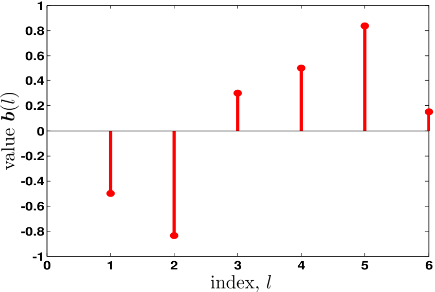
As a visualization aid, an arbitrary vector in the canonical-sparse cone is shown in Fig. 1. A couple of comments about the premise of Theorem 2 are in order. Let denote an unidentifiable pair in the feasible set of Theorem 2.
- 1.
Our proof technique hinges on an adversarial construction of and . By feasibility of , needs to be satisfied, which might conflict with our adversarial construction if or holds. Clearly, both of these scenarios are rendered impossible, if we insist on and .
- 2.
We insist on and to have a strictly non-trivial realization of the sparse blind deconvolution problem, i.e. an instance which violates some assumption of Theorem 1 other than model orders and being even. It is easy to see that if in (6) then admits a non-zero dimensional Lebesgue measure. Hence, if either or is empty in Theorem 2, then the sparse blind deconvolution problem instance so generated will fall under the purview of Theorem 1 (assuming even and ). Technically speaking, Theorem 2 is valid even if or is empty (provided that ), however its implications are weaker than that of Theorem 1 when and are even. Furthermore, note that the requirements and respectively imply and .
We note that the assumptions of Theorem 2 imply and so that the unidentifiable subset of is at least 5 dimensional. In particular, the unidentifiable set in Theorem 2 is always non-trivial. We also note that the canonical-sparse feasible domain of Theorem 2 is far more structured than the feasible set of Theorem 1 and hence, the set of all unidentifiable inputs in Theorem 2 is much smaller. Nonetheless, the canonical-sparsity structure is not strong enough to guarantee identifiability for all canonical-sparse vectors. Additionally, note that and denote sets of zero indices, so that larger cardinality of or implies a sparser problem instance. Furthermore, we note that Corollary 1 straightforwardly follows from Theorem 2 by setting and . However, the result in Corollary 1 is not tight for being an even integer. We remedy this shortcoming in Section III-C by directly specializing Theorem 1 to (the feasible set of Corollary 1) to yield Corollary 2.
Exploiting the equivalence between bilinear inverse problems and rank one matrix recovery problems [20] (in the current context, equivalence between Problems (P1) and (P2)) the result of Theorem 2 can be interpreted as evidence of the null space of the convolution operator admitting a large number of simultaneously canonical-sparse and low-rank matrices. For rank one matrix completion problems [34], it is relatively straightforward to see that a random sampling operator on a sparse rank one matrix will return zeros on most samples, thus rendering it impossible to distinguish the rank one matrix in question from the all zero matrix. However, the same observation is not at all straightforward for a rank one matrix recovery problem [35] when the sampling operator is fixed to the lifted linear convolution operator. Theorem 2 asserts that this is indeed true and the lifted linear convolution operator admits a large number of non-zero canonical-sparse matrices within its rank two null space.
It is important to note that Theorems 1 and 2 are of different flavors and are not comparable since they make different assumptions on the feasible domain. In particular, neither theorem universally implies the other even if we consider special cases for each of them. To make this point more explicit, we make the following observations.
- 1.
- 2.
In Theorem 2, even if we assume the model orders and to be even and the zero index sets and to be empty (so that the feasible set is equal to almost everywhere w.r.t. the dimensional Lebesgue measure), we can only draw the conclusion that there exists a dimensional unidentifiable subset (call it ) of the feasible set. This is clearly insufficient to show almost everywhere unidentifiability (as claimed by Theorem 1) since the complement of could be a dimensional set as well, admitting non-zero dimensional Lebesgue measure.
- 3.
If is considered with even model orders so that the feasible sets in Theorems 1 and 2 are equal almost everywhere w.r.t. the dimensional Lebesgue measure, then the conclusion of Theorem 1 is stronger, since almost everywhere unidentifiability over automatically implies the existence of a dimensional unidentifiable subset.
Subsection III-C A Mixed Extension
It is possible to fuse the ideas from Theorems 1 and 2 to strengthen the conclusion of Corollary 1 on the domain , i.e. on a domain formed by the Cartesian product of a canonical-sparse and a non-sparse cone.
Corollary 2.
Let be an arbitrary integer and be an even integer. For any given index set , let and define . Then there exists a set of dimension such that , is unidentifiable almost everywhere w.r.t. any measure over that is absolutely continuous w.r.t. the dimensional Lebesgue measure.
Proof:
Appendix B. ∎
Note that Corollary 2 is a non-trivial extension of Theorem 1, since Definition 1 defines identifiability of an input signal pair within some feasible set and this set is different for Theorem 1 and Corollary 2. In particular, if is an unidentifiable pair in the feasible set of Corollary 2, then the proof of the result involves the construction of a candidate adversarial input as in Theorem 2 as well as the vector as in Theorem 1.
Through the unidentifiability results in this section, we have attempted to quantify the ill-posedness of blind deconvolution under canonical-sparsity constraints, and illustrate the geometric reasons behind this unfavorable sparsity-ambiguity trade-off behavior. The rule of thumb for determining the sparsity-ambiguity trade-off for canonical-sparse blind deconvolution is well illustrated by comparing the conclusions of Theorem 1 and Corollary 2. Roughly speaking, if the set of zero indices for the signal vector has cardinality then the dimension of the set of unidentifiable choices for is reduced from in Theorem 1 to somewhere between and in Corollary 2. The main message is that if an application exhibits a bilinear observation model of linear convolution and the additional application specific structure is that of canonical sparsity of the unknown variables, then it is necessary to drastically revise the system design specifications for any hope of signal identifiability. Such revision may incorporate some form of randomized precoding of the unknowns, so that the effective bilinear operator governing the observation model looks substantially different from the convolution operator (e.g. the Gaussian random precoding used in [5]). Alternatively, sparsity in non-canonical bases could also be helpful (e.g. Rademacher random vector signal model used in [20] and the constant modulus based problem instances in [14]).
Section IV Unidentifiability Results with Coding
Structural information about unknown input signals is almost exclusively a result of specific application dependant data or system deployment architectures. In this section, we consider an abstraction for a problem in multi-hop channel estimation [22, 21] and analyze other subspace based structural priors relevant to this application. Studying constrained adversarial realizations of these abstractions has utility far beyond communication systems. For example, when communication subsystems are parts of a larger complex system involving sensing and navigation for autonomous vehicles [36, 37, 38, 39, 40] then non-linear inter-system interactions may become unavoidable. In this section, we extend our unidentifiability results from Section III to simple forms of coding across the transmitters for the second-hop channel estimation problem. Section IV-A considers the somewhat idealized, but simpler to interpret, scenario of repetition coding across transmitters and states unidentifiability results for both unstructured as well as canonical-sparse channels. Rather than explicitly proving the results in Section IV-A, we note that they are important special cases of the more general unidentifiability result in Section IV-B for certain families of partially cooperative codes (Theorem 3) that we prove in Appendix C. Finally, Corollary 6 states yet another important special case of Theorem 3 pertaining to geometrically decaying subspace sparse signals, previously considered in [2]. In the spirit of using commonly employed notation, we shall denote the unknown pair by the pair with pertaining to a topological configuration of the network and representing the channel impulse response as described next.

In a previous paper [21], we developed a structured channel model based on the multichannel approximation for the second hop in a relay assisted communication topology shown in Fig. 2. Specifically, we consider relays R1, R2, …, R and let denote the propagation delay and power adjusted SISO channel impulse response (CIR) common to each relay-destination R D channel, . Thus, the effective CIR at the destination is formed by a superposition of distinct delayed scalar multiples of the vector . If the maximum propagation delay of R relative to R1 is upper bounded by , then there exists a vector and an index subset (with ) such that the propagation delay adjusted SISO CIR for the R D channel is and that , . With these definitions and letting denote the Toeplitz matrix representation for delay by units , the effective CIR at the destination is given by the linear convolution and the channel estimation problem at the destination is to recover the vector pair from the observation of . Since the vectors and are not arbitrary, but have physical interpretations leading to structural restrictions, we can incorporate this knowledge by a constraint of the form of for some set . For example, if represents a SISO CIR for underwater acoustic communication [41, 42] (or, more generally, for wide-band communication [43]), then has been observed to exhibit canonical-sparsity. Now, associating the pair with a feasible solution to Problem (P1), the success of the channel estimation problem at the destination is critically contingent upon the identifiability of as a solution to Problem (P1) by the criterion in Definition 1.
As with our prior results, herein we shall consider to be a separable cone in with and . In many applications, it is typical to have (respectively ) to be a low-dimensional subset of (respectively ). An important interpretation of is that can be considered as a coded representation (of ambient dimension ) of the unknown whose actual dimension is much smaller (equal to that of the Hausdorff dimension of ). However, this coded representation is invoked to help strengthen the identifiability properties of the problem, rather than to help with error correction in the presence of observation noise. This is a somewhat different interpretation of coding than the classical goal of correcting noise induced errors. Operationally, both interpretations rely on redundancy albeit for different purposes.
Subsection IV-A Repetition Coding
Suppose that a few of the relays in Fig. 2 cooperatively decide to maintain the same relative transmission powers and phases and this decision is communicated to the destination for use as side information for channel estimation. A physical motivation for allowing few rather than all relays to cooperate, may be attributed to infeasibility of such coordination for widely separated relays and/or for a large number of relays. Mathematically, this translates to the use of a smaller feasible set by virtue of a stricter structural restriction on via the set that is smaller than . Specifically, let be the index set of propagation delays corresponding to the cooperating relays. Assuming that the only structure on is that induced by the cooperating relays, we define the repetition coded domain as where act as parameters to the following parametrized definition of a family of cones for any dimension and any index set ,
| (16) |
In other words, the set imposes the structure that each of its member vectors has the same non-zero value on the index subset ; the value of being allowed to vary across members. Even for a large number of cooperating relays (as measured by the cardinality ), Corollaries 3 and 4 stated below imply unidentifiability results for (unstructured channel) and (canonical-sparse channel), respectively. Corollary 3 makes a statement for the repetition coded domain that is analogous to the conclusions drawn by Corollary 1 for the canonical-sparse domain . The main technical difference between Corollaries 3 and 1 is that they require different constructions for a candidate unidentifiable input signal since the feasible domain is different across these results. We defer further technical details to the proof of Theorem 3 in Appendix C. Corollary 4 can be interpreted as extending the unidentifiability results of Theorem 2 from the canonical-sparse product domain to the mixed product of repetition coded and canonical-sparse domains . Roughly speaking, because we only consider separable domains , one can simply fuse the different constructions of a candidate adversarial signal from Corollary 3 and from Corollary 1 to produce a candidate unidentifiable pair for Corollary 4. This ability to fuse individual adversarial signal constructions on sets and to produce candidate unidentifiable signal pairs within the Cartesian product domain underlies the simplicity of arguments in the proof of Theorem 3. At present, we cannot foresee any adaptations to the constructions used in the proof of Theorem 3 that would allow us to make analogous statements for non-separable domains in a generalizable way.
Corollary 3.
Let and be arbitrary integers. For any given index set , let and define . Then there exists a set such that every is unidentifiable. If then is of dimension at least , otherwise is of dimension at least .
Corollary 4.
Let and be arbitrary integers. For any given index sets and , let and let and . Then there exists a set such that every is unidentifiable. If then is of dimension at least , otherwise is of dimension at least .
We note that in contrast to the results for the canonical-sparse domain in Corollary 1, the dimension of unidentifiable subset for the repetition coded domain as given by Corollary 3 depends on whether is non-empty, i.e. if atleast one pair of adjacent indices for are repetition coded and hence belong to . Corollary 4 essentially says that even with a canonical-sparse prior structure on the channel vector and nearly full cooperation between intermediate relays () via repetition coding on , there may be non-zero dimensional unidentifiable signal subsets in the feasible domain . We recall that the index subsets and in Corollary 4 are known at the receiver and the unidentifiable signal set exists despite the availability of this side information. Thus, the repetition coding based system architecture laid out in this section is bound to fail in practice although it may be an intuitive choice. An important implication of Corollary 4 is that it is necessary to have , which is equivalent to the requirement that either the first relay or the last relay (when ordered by increasing propagation delays) must be present in the cooperating subset of relays.
Subsection IV-B Partially Cooperative Coding
The results in Section IV-A can be generalized to other codes. Consider the system described in Section IV-A, except that the cooperating relays decide on a different structural restriction for . As before, let denote the index set of propagation delays corresponding to the cooperating relays. We let denote a partially cooperative coded domain where the vector denotes the cooperative code (alternatively, could also be interpreted as a power-delay-profile across cooperating relays) and are specific parameters to the following parametrized definition of a family of cones for any dimension and any index set ,
| (17) |
As a visual example, Fig. 3 shows an arbitrary vector in the partially cooperative coded domain for the code vector . It is important to note that the code vector is known at the destination so that the decoder has explicit knowledge of the set . Furthermore, the partially cooperative coded domain unifies and generalizes both the repetition coded domain and the canonical-sparse domain . To see this, we first note that implies by definition, and that the definitions (16) and (17) are equivalent for . Secondly, if the code vector admits a partition of the form for some disjoint index subsets , then the definitions in (17), (16) and (6) would imply that . This can be checked directly by substitution.

Corollary 5 and Theorem 3 stated below imply unidentifiability results for certain joint properties of the pair, i.e. for certain joint configurations of the cooperating relay index set and the cooperative code employed. The unidentifiability results may hold for both (unstructured channel) and (subspace-sparse channel), even for a large number of cooperating relays (as measured by the cardinality ). In what follows, denotes the Minkowski sum of the sets and .
Corollary 5.
Let and be arbitrary integers. For any given index set , let , and define . If , then there exists a set of dimension at least , such that every is unidentifiable. Otherwise, if then denote by , the index subset such that , is collinear with . If and are collinear, then there exists a set of dimension at least , such that every is unidentifiable.
Corollary 5 makes a statement for the partially cooperative coded domain that is essentially analogous to the statement of Corollary 3 for the repetition coded domain , the only technical distinction being a more elaborate specification of the unidentifiable configurations of the pair in the former result. Some of the technical conditions on the pair , for generating unidentifiable configurations, are automatically satisfied when and hence we chose to present this simpler instantiation of Corollary 5 in the form of Corollary 3 under the rubric of repetition coding in the last subsection. In particular, both domains and share the same construction for a candidate unidentifiable input signal, provided the premise of Corollary 5 is satisfied. Furthermore, Corollaries 1, 3 and 5 motivate the following categorization of the pairs in preparation for the statement of Theorem 3.
Definition 2.
Let be an arbitrary integer, be a given index set and be a code vector. Let . The following mutually exclusive (but not exhaustive) categories for the pair are defined.
- 0.
If , and then is of type 0.
- 1.
Let and . If is collinear with then is of type 1. If is not collinear with then let denote the index subset such that , is collinear with . If and are collinear, then is of type 1.
- 2.
If and then is of type 2.
For a visual example, we note that Fig. 1 represents a pair of type 0 while Fig. 3 shows a type 1 pair with ( as defined above in Definition 2).
Theorem 3.
Let be arbitrary integers. For any given index sets and , let and let and . If the pairs and are respectively of types and for , then there exists a set of dimension at least such that every is unidentifiable.
Proof:
Appendix C. ∎
Theorem 3 stated above utilizes the construction of candidate adversarial inputs over different domains, as developed in Corollaries 1 and 5, and fuses them together to generate candidate unidentifiable signal pairs by exploiting the separability of the feasible domain . It is straightforward to check that Theorem 2 and Corollaries 1, 3, 4, and 5 can all be derived from Theorem 3 by suitable choices of the parameter pairs and , e.g. setting and gives back Corollary 4. In essence, barring Corollary 2 which requires special assumptions, Theorem 3 encompasses all of the unidentifiability results for constrained blind deconvolution developed in this part of the paper.
The main message of Theorem 3 is that the coded subspaces represented by the vectors and are critical to the identifiability of the blind linear deconvolution problem (P1). If these coded subspaces are solely determined by the application or natural system configuration (like the multi-hop channel estimation example above) then sparsity may not be sufficient to guarantee identifiability for the blind deconvolution problem. A certain amount of design freedom on both of the coded subspaces (represented by vectors and ) is necessary to guarantee identifiability under blind deconvolution (like in [5, 20, 14]).
As yet another important special case for wireless communications, we interpret the vector as a power-delay profile and assume it to be geometrically decaying over some contiguous index subset , i.e. satisfies for some and all . Then we get the geometrically decaying cone of all -dimensional real vectors that are geometrically decaying on the index subset and it admits the following unidentifiability result (in the statement below, represents a geometrically decaying cone).
Corollary 6.
Let and be arbitrary integers. For any given index subset and any contiguous index subset , let and define , . Then there exists a set such that every is unidentifiable. If then is of dimension at least , otherwise is of dimension at least .
We omit the proof of Corollary 6 here as it follows from specializing the proof of Theorem 3. A complete proof of Corollary 6 appears in our earlier work [2]. The occurrence of a geometrically decaying power-delay profile is common in underwater acoustic communication channels [44] and more generally in wide-band communication channels [45, 46].
Section V Conclusions
Blind deconvolution is an important non-linear inverse problem commonly encountered in signal processing applications. Natively, blind deconvolution is ill-posed from the viewpoint of signal identifiability and it is assumed that application specific additional constraints (like sparsity) would suffice to guarantee identifiability for this inverse problem. In the current work, we showed that (somewhat surprisingly) sparsity in the canonical basis is insufficient to guarantee identifiability under fairly generic assumptions on the support of the sparse signal. Specifically, we explicitly demonstrate a form of rotational ambiguity that holds true for sparse vectors as well. Our approach builds on the lifting technique from optimization to reformulate blind deconvolution into a rank one matrix recovery problem, and analyzes the rank two null space of the resultant linear operator. While this approach is philosophically applicable to other bilinear inverse problems (like dictionary learning), it is the simplicity of the convolution operator in the lifted domain that makes our analysis tractable. We developed scaling laws quantifying the ill-posedness of canonical-sparse blind deconvolution by bounding the dimension of the unidentifiable sparse signal set. When applied to a second-hop sparse channel estimation problem, our methods also revealed the insufficiency of side information involving repetition coding or geometrically decaying signals towards guaranteeing identifiability under blind linear deconvolution. To establish our results, we developed a measure theoretically tight, partially parametric and partially recursive characterization of the rank two null space of the linear convolution map. This result is a precursor to non-randomized code design strategies for guaranteeing signal identifiability under the bilinear observation model of linear convolution. The design of such codes is a topic of ongoing research.
References
- [1] S. Choudhary and U. Mitra, “Sparse Blind Deconvolution: What Cannot Be Done,” in 2014 IEEE International Symposium on Information Theory (ISIT), Honolulu, USA, Jun. 2014, pp. 3002–3006.
- [2] ——, “On The Impossibility of Blind Deconvolution for Geometrically Decaying Subspace Sparse Signals,” in 2nd IEEE Global Conference on Signal and Information Processing (GlobalSIP), Atlanta, USA, Dec. 2014, pp. 463–467.
- [3] J. Hadamard, “Sur les problèmes aux dérivées partielles et leur signification physique,” Princeton University Bulletin, vol. 13, no. 28, pp. 49–52, 1902.
- [4] A. N. Tikhonov and V. Y. Arsenin, Metody resheniya nekorrektnykh zadach, 3rd ed. “Nauka”, Moscow, 1986.
- [5] A. Ahmed, B. Recht, and J. Romberg, “Blind deconvolution using convex programming,” IEEE Trans. Inf. Theory, vol. 60, no. 3, pp. 1711–1732, 2014.
- [6] A. Kammoun, A. Aissa El Bey, K. Abed-Meraim, and S. Affes, “Robustness of blind subspace based techniques using quasi-norms,” in 2010 IEEE Eleventh International Workshop on Signal Processing Advances in Wireless Communications (SPAWC), 2010, pp. 1–5.
- [7] K. Herrity, R. Raich, and A. O. Hero, III, “Blind Reconstruction of Sparse Images with Unknown Point Spread Function,” Computational Imaging VI, vol. 6814, no. 1, p. 68140K, 2008.
- [8] D. Barchiesi and M. D. Plumbley, “Dictionary Learning of Convolved Signals,” in 2011 IEEE International Conference on Acoustics, Speech and Signal Processing (ICASSP), May 2011, pp. 5812–5815.
- [9] C. Hegde and R. G. Baraniuk, “Sampling and Recovery of Pulse Streams,” IEEE Trans. Signal Process., vol. 59, no. 4, pp. 1505–1517, 2011.
- [10] P. D. O’Grady, B. A. Pearlmutter, and S. T. Rickard, “Survey of sparse and non-sparse methods in source separation,” International Journal of Imaging Systems and Technology, vol. 15, no. 1, pp. 18–33, 2005.
- [11] S. Choudhary and U. Mitra, “Fundamental Limits of Blind Deconvolution Part I: Ambiguity Kernel,” ArXiv e-prints, vol. abs/1411.3810, Nov. 2014. [Online]. Available: http://arxiv.org/abs/1411.3810
- [12] D. L. Donoho, “Compressed Sensing,” IEEE Trans. Inf. Theory, vol. 52, no. 4, pp. 1289–1306, 2006.
- [13] K. Abed-Meraim, W. Qiu, and Y. Hua, “Blind System Identification,” Proc. IEEE, vol. 85, no. 8, pp. 1310–1322, Aug. 1997.
- [14] C. R. Johnson, Jr., P. Schniter, T. J. Endres, J. D. Behm, D. R. Brown, and R. A. Casas, “Blind Equalization Using the Constant Modulus Criterion: A Review,” Proc. IEEE, vol. 86, no. 10, pp. 1927–1950, Oct. 1998.
- [15] H. Liu, G. Xu, L. Tong, and T. Kailath, “Recent developments in blind channel equalization: From cyclostationarity to subspaces,” Signal Processing, vol. 50, no. 1, pp. 83–99, 1996, special Issue on Subspace Methods, Part I: Array Signal Processing and Subspace Computations.
- [16] J. H. Manton and W. D. Neumann, “Totally blind channel identification by exploiting guard intervals,” Systems & Control Letters, vol. 48, no. 2, pp. 113–119, 2003.
- [17] M. S. Asif, W. Mantzel, and J. K. Romberg, “Random Channel Coding and Blind Deconvolution,” in 47th Annual Allerton Conference on Communication, Control, and Computing (Allerton), Sep. 2009, pp. 1021–1025.
- [18] S. Choudhary and U. Mitra, “On Identifiability in Bilinear Inverse Problems,” in 2013 IEEE International Conference on Acoustics, Speech and Signal Processing (ICASSP), Vancouver, Canada, May 2013, pp. 4325–4329.
- [19] ——, “Identifiability Bounds for Bilinear Inverse Problems,” in 47th Asilomar Conference on Signals, Systems and Computers, Pacific Grove, USA, Nov. 2013, pp. 1677–1681.
- [20] ——, “Identifiability Scaling Laws in Bilinear Inverse Problems,” ArXiv e-prints, vol. abs/1402.2637, Feb. 2014. [Online]. Available: http://arxiv.org/abs/1402.2637
- [21] N. Richard and U. Mitra, “Sparse Channel Estimation for Cooperative Underwater Communications: A Structured Multichannel Approach,” in 2008 IEEE International Conference on Acoustics, Speech and Signal Processing (ICASSP), Mar. 2008, pp. 5300–5303.
- [22] S. Choudhary and U. Mitra, “Sparse recovery from convolved output in underwater acoustic relay networks,” in 2012 Asia-Pacific Signal Information Processing Association Annual Summit and Conference (APSIPA ASC), Hollywood, USA, Dec. 2012, pp. 1–8.
- [23] N. Michelusi, U. Mitra, A. F. Molisch, and M. Zorzi, “Hybrid sparse/diffuse channels: A new model and estimators for wideband channels,” in 49th Annual Allerton Conference on Communication, Control, and Computing (Allerton), Sep. 2011, pp. 477–484.
- [24] D. Barchiesi and M. D. Plumbley, “Learning Incoherent Dictionaries for Sparse Approximation Using Iterative Projections and Rotations,” IEEE Trans. Signal Process., vol. 61, no. 8, pp. 2055–2065, Apr. 2013.
- [25] R. Tur, Y. C. Eldar, and Z. Friedman, “Innovation rate sampling of pulse streams with application to ultrasound imaging,” IEEE Trans. Signal Process., vol. 59, no. 4, pp. 1827–1842, 2011.
- [26] P. Jung and P. Walk, “Sparse Model Uncertainties in Compressed Sensing with Application to Convolutions and Sporadic Communication,” ArXiv e-prints, vol. abs/1404.0218, Apr. 2014. [Online]. Available: http://arxiv.org/abs/1404.0218
- [27] R. Gribonval and K. Schnass, “Dictionary identification—sparse matrix-factorization via -minimization,” IEEE Trans. Inf. Theory, vol. 56, no. 7, pp. 3523–3539, 2010.
- [28] K. Jaganathan, S. Oymak, and B. Hassibi, “Sparse Phase Retrieval: Convex Algorithms and Limitations,” in 2013 IEEE International Symposium on Information Theory Proceedings (ISIT), Jul. 2013, pp. 1022–1026.
- [29] A. Fannjiang, “Absolute uniqueness of phase retrieval with random illumination,” Inverse Problems, vol. 28, no. 7, pp. 075 008, 20, 2012.
- [30] E. J. Candès, Y. C. Eldar, T. Strohmer, and V. Voroninski, “Phase retrieval via matrix completion,” SIAM J. Imaging Sci., vol. 6, no. 1, pp. 199–225, 2013.
- [31] E. Balas, “Projection, lifting and extended formulation in integer and combinatorial optimization,” Ann. Oper. Res., vol. 140, pp. 125–161, 2005.
- [32] A. Beck, “Convexity properties associated with nonconvex quadratic matrix functions and applications to quadratic programming,” J. Optim. Theory Appl., vol. 142, no. 1, pp. 1–29, 2009.
- [33] P. Mattila, Geometry of sets and measures in Euclidean spaces, Fractals and rectifiability, ser. Cambridge Studies in Advanced Mathematics. Cambridge University Press, Cambridge, 1995, vol. 44.
- [34] E. J. Candès and B. Recht, “Exact matrix completion via convex optimization,” Found. Comput. Math., vol. 9, no. 6, pp. 717–772, 2009.
- [35] D. Gross, “Recovering Low-Rank Matrices From Few Coefficients in Any Basis,” IEEE Trans. Inf. Theory, vol. 57, no. 3, pp. 1548–1566, 2011.
- [36] G. Hollinger, S. Choudhary, P. Qarabaqi, C. Murphy, U. Mitra, G. Sukhatme, M. Stojanovic, H. Singh, and F. Hover, “Communication protocols for underwater data collection using a robotic sensor network,” in 2011 IEEE GLOBECOM Workshops (GC Wkshps), Houston, USA, Dec. 2011, pp. 1308–1313.
- [37] S. Choudhary, N. Kumar, S. Narayanan, and U. Mitra, “Active Target Detection with Mobile Agents,” in 2014 IEEE International Conference on Acoustics, Speech and Signal Processing (ICASSP), Florence, Italy, May 2014, pp. 4218–4222.
- [38] G. A. Hollinger, U. Mitra, and G. S. Sukhatme, “Autonomous Data Collection from Underwater Sensor Networks using Acoustic Communication,” in 2011 IEEE/RSJ International Conference on Intelligent Robots and Systems (IROS), Sep. 2011, pp. 3564–3570.
- [39] L. Freitag, M. Johnson, M. Grund, S. Singh, and J. Preisig, “Integrated Acoustic Communication and Navigation for Multiple UUVs,” in OCEANS, 2001. MTS/IEEE Conference and Exhibition, vol. 4, Nov. 2001, pp. 2065–2070.
- [40] S. Choudhary, D. Kartik, N. Kumar, S. Narayanan, and U. Mitra, “Active Target Detection with Navigation Costs: A Randomized Benchmark,” in 52nd Annual Allerton Conference on Communication, Control, and Computing (Allerton), Monticello, USA, Sep. 2014, pp. 109–115.
- [41] C. R. Berger, S. Zhou, J. C. Preisig, and P. Willett, “Sparse Channel Estimation for Multicarrier Underwater Acoustic Communication: From Subspace Methods to Compressed Sensing,” IEEE Trans. Signal Process., vol. 58, no. 3, pp. 1708–1721, Mar. 2010.
- [42] W. Li and J. Preisig, “Estimation of Rapidly Time-Varying Sparse Channels,” IEEE J. Ocean. Eng., vol. 32, no. 4, pp. 927–939, Oct. 2007.
- [43] A. F. Molisch, “Ultra-Wide-Band Propagation Channels,” Proc. IEEE, vol. 97, no. 2, pp. 353–371, Feb. 2009.
- [44] N. Michelusi, B. Tomasi, U. Mitra, J. Preisig, and M. Zorzi, “An evaluation of the hybrid sparse/diffuse algorithm for underwater acoustic channel estimation,” in OCEANS 2011, Sep. 2011, pp. 1–10.
- [45] A. Molisch, D. Cassioli, C.-C. Chong, S. Emami, A. Fort, B. Kannan, J. Karedal, J. Kunisch, H. Schantz, K. Siwiak, and M. Win, “A Comprehensive Standardized Model for Ultrawideband Propagation Channels,” IEEE Trans. Antennas Propag., vol. 54, no. 11, pp. 3151–3166, Nov. 2006.
- [46] A. Saleh and R. Valenzuela, “A Statistical Model for Indoor Multipath Propagation,” IEEE J. Sel. Areas Commun., vol. 5, no. 2, pp. 128–137, Feb. 1987.
Appendix A Proof of Theorem 2
The proof relies on constructing a generative model for vectors and such that is unidentifiable within . Let , , and be chosen arbitrarily, where
| (18) |
We use the 4-tuple to generate the vector pair using
| (19) |
and the vector pair using
| (20) |
By assumption, and , so (19) implies and (20) implies . We also have and by assumption, and
| (21a) | ||||
| as well as | ||||
| (21b) | ||||
where (21a) follows from (19) and (21b) follows from (20). Therefore, and , implying that . Setting , we have
| (22) |
and hence, from Lemma 1. Therefore, the pairs and produce the same convolved output and are indistinguishable under the linear convolution map. Since and are linearly independent by the choice , is unidentifiable by Definition 1 with as the certificate of unidentifiability.
All that remains is to lower bound the dimension of a set of pairs that can be shown to be unidentifiable for blind linear deconvolution using the above mentioned construction. Let denote the Cartesian product set . We construct as follows. A vector pair if and only if all of the following conditions are satisfied.
- (A1)
is generated from a 4-tuple using (19).
- (A2)
.
- (A3)
.
From the arguments in the previous paragraph, we have and furthermore, every is unidentifiable within . Let us consider the sets
| (23) |
By the definition in (6), is a dimensional Borel subset of , and is a dimensional Borel subset of . Further, is a one dimensional Borel subset of and given a value of , is also a one dimensional Borel subset of . Hence, (23), (A2) and (A3) imply that
- 1.
is a dimensional Borel subset of ,
- 2.
given , is a dimensional Borel subset of ,
- 3.
is a two dimensional Borel subset of , and
- 4.
is a dimensional Borel subset of .
Next, we compute the dimension of the set . Consider a factorization of into
| (24) |
i.e. . Equations (24) and (19) imply that every is generated as the result of a uniformly continuous map from (with a non-singular Jacobian matrix). From Lemma 2, the quotient set is finite for every and therefore each can be generated by at most a finite number of elements using (19). Given some , let be a set such that for every , there exists generating using (19). Clearly, from Lemma 2. Then, (24) and (19) imply that every is generated as the result of a uniformly continuous map from (with a non-singular Jacobian matrix). Using Lemma 2, the quotient set is finite for every and therefore each can be generated by at most a finite number of elements using (19). Since is a finite set, the above arguments and (24) imply that every element is generated by at most a finite number of 4-tuples , using the uniformly continuous maps in (19) (with non-singular Jacobian matrices). Since is a dimensional Borel subset of , we get as a Borel subset of of dimension .
We let , i.e. is the quotient set of w.r.t. the equivalence relation . Clearly, . Since each element is a representative for a one dimensional Borel subset , the dimension of is one less than the dimension of . Hence, is a dimensional set.
Appendix B Proof of Corollary 2
This proof follows the template of the proof for Theorem 2 in Appendix A with adjustments for the change of feasible set and borrows from the proof of Theorem 1 in Part I of the paper to show almost everywhere unidentifiability.
Let and be arbitrarily chosen. Since is an even integer, invoking Lemma 2 for yields a vector and a scalar such that the second relationship in (19) is satisfied. Next, we select and use the parameters in (19) to generate the vector . We reuse the parameter 4-tuple in (20) to generate the pair . Note that our construction for the 4-tuple here is different from that in Appendix A, even if we set in Theorem 2. Nonetheless, using (22) and reasoning on the same lines as in Appendix A leads to the conclusion that is unidentifiable with as the certificate of unidentifiability.
For notational brevity, let us define
| (25) |
To show that given any , almost every choice of yields an unidentifiable pair , it suffices to show that holds almost everywhere w.r.t. the measure over . From (19), the dependence of is uniformly continuous on the real numbers and these real numbers completely parametrize . Further, since the measure over is absolutely continuous w.r.t. the dimensional Lebesgue measure, it is possible to choose a measure over that is absolutely continuous w.r.t. the one dimensional Lebesgue measure. Since is a zero dimensional set (given the value of ), is true almost everywhere w.r.t. the measure over and therefore also w.r.t. the measure over .
Let denote the image of under the map in (19). To complete the proof, we need to bound the dimension of the set . Analogous to Appendix A, we have as a dimensional Borel subset of and therefore, is a dimensional Borel subset of . For any , Lemma 2 implies the finiteness of the quotient set and therefore each can be generated by at most a finite number of elements using (19). Since (19) represents uniformly continuous maps with non-singular Jacobian matrices, we have as a dimensional Borel subset of . The proof is complete since for any , is unidentifiable almost everywhere w.r.t. any measure over that is absolutely continuous w.r.t. the dimensional Lebesgue measure.
Appendix C Proof of Theorem 3
For notational convenience, we denote by , by , by , and by . The high level architecture of this proof is similar to the proof of Theorem 2 in Appendix A. However, the generative model for unidentifiable pairs is substantially different, owing to the change in the feasible set .
We shall use (19) to construct unidentifiable pairs in the separable feasible set . Since the generative parameters for and in (19) are disjoint, an analogous construction also works for the feasible set to produce unidentifiability results. For example, Corollary 4 asserts that for and , there exists an unidentifiable subset of of dimension . Our reasoning based on disjoint generation would imply that for and , there exists an unidentifiable subset of of dimension . Thus, it suffices to consider unordered pairs for the purpose of this proof. Note that Theorem 2 is exactly equivalent to the case of . In the rest of the proof, we complete the treatment for the remaining cases .
Let us choose the 4-tuple of parameters such that we generate from (19) and from (20). For the construction to be consistent, must satisfy
| (26a) | ||||
| (26b) | ||||
for some scalars that could depend on , and . Solving (26) for and , we get
| (27a) | ||||
| (27b) | ||||
Analogously, consistency also requires to satisfy
| (28a) | ||||
| (28b) | ||||
for some scalars that could depend on , and . Solving (28) for and , we get
| (29a) | ||||
| (29b) | ||||
Given a value of ( is defined in (18)), if there exist solutions to satisfying (27) and satisfying (29), then the construction of is consistent. Invoking (22) and using the same line of reasoning as in Appendix A implies that is unidentifiable with as the certificate of unidentifiability. Furthermore, the consistency condition (27) for is independent of the consistency condition (29) for for a given . Thus, it suffices to analyze the cases for different values of and the same analysis would apply to the cases owing to the similarity between (27) and (29).
If is of type , the analysis in Appendix A can be reused. In particular, we have and (27) reduces to the requirement . Clearly, any is a valid assignment and is a dimensional Borel subset of for .
If is of type , then and there are no common variables between the vectors and . Thus, any will yield a consistent assignment for through (27) with arbitrary constants and satisfying and . Clearly, for , there is a two dimensional set of valid choices for the pair and therefore and lie (independently of each other) on a one dimensional subspace collinear with , implying that lies on a two dimensional subspace of . Since is unconstrained , the set of consistent assignments of is a Borel subset of of dimension at least .
Finally, let us analyze the case when is of type . We have , so must receive consistent assignments from (27a) and (27b). If is collinear with , then (27) is consistent if and only if and
| (30) |
If is not collinear with , then there exists an index subset as characterized in Definition 2. Further, (27a) and (27b) respectively imply (31a) and (31b) below.
| (31a) | ||||
| (31b) | ||||
Since is of type , and are collinear and there exists a constant such that . The consistency requirement in (31) then reduces to requiring and
| (32) |
Note that (32) subsumes (30) (on setting ), and further implies
| (33) |
for . We define the set as
| (34) |
and notice that for any , and (33) implies that the set of valid choices for the pair is one dimensional. Therefore, it follows from (27) and (31) that lies on a one dimensional subspace of and is given by
| (35) |
for some scalar . In the special case when is collinear with , (35) simplifies to being collinear with . Since is unconstrained , the set of consistent assignments of is a Borel subset of of dimension at least , for any .
For notational brevity, we define the following. Let (respectively ) denote the set of all vectors (respectively ) that satisfy the consistency condition (27) and (respectively (29) and ) for a given value of . Moreover, let denote the largest set of allowed values for the pair depending on the type pair of the pairs and . In particular,
- 1.
implies ,
- 2.
implies , and
- 3.
implies , where depends on in the same way as depends on .
Finally, let denote the image of the set under the map in (19). Clearly, and every is unidentifiable within if (27) and (29) can be simultaneously satisfied with . Our analysis indeed guarantees this using Definition 2 and careful descriptions for the sets , , and the conic family in (17).
To finish the proof, we need to compute the dimension of . Our analysis for the cases establishes that is a dimensional Borel set and (by analogy) is a dimensional Borel set. Clearly, is a two dimensional Borel set for any . Therefore, is a dimensional Borel subset of . Since is the concatenated image of the uniformly continuous maps in (19) (with non-singular Jacobian matrices), invoking Lemma 2 as in Appendix A implies that is a dimensional Borel set. Setting and invoking the argument in the last paragraph of Appendix A implies that the dimension of is one less than the dimension of and completes the proof.