On the Complexity of Parallel Coordinate Descent
Abstract
In this work we study the parallel coordinate descent method (PCDM) proposed by Richtárik and Takáč [26] for minimizing a regularized convex function. We adopt elements from the work of Lu and Xiao [39], and combine them with several new insights, to obtain sharper iteration complexity results for PCDM than those presented in [26]. Moreover, we show that PCDM is monotonic in expectation, which was not confirmed in [26], and we also derive the first high probability iteration complexity result where the initial levelset is unbounded.
1 Introduction
Block coordinate descent methods are being thrust into the optimization spotlight because of a dramatic increase in the size of real world problems, and because of the “Big data” phenomenon. It is little wonder, when these seemingly simple methods, with low iteration costs and low memory requirements, can solve problems where the dimension is more than one billion, in a matter of hours [26].
There is an abundance of coordinate descent variants arising in the literature including: [4, 6, 9, 11, 12, 15, 16, 22, 24, 27, 28, 31, 32, 33, 34, 35, 36, 37, 38]. The main differences between these methods is the way in which the block of coordinates to update is chosen, and also how the subproblem to determine the update to apply a block of variables is to be solved. The current, state-of-the-art block coordinate descent method is the Parallel (block) Coordinate Descent Method (PCDM) of Richtárik and Takáč [26]. This method selects the coordinates to update randomly and the update is determined by minimizing an overapproximation of the objective function at the current point (see Section 3 for a detailed description). PCDM can be applied to a problem with a general convex composite objective, it is supported by strong iteration complexity results to guarantee the method’s convergence, and it has been tested numerically on a wide range of problems to demonstrate its practical capabilities.
In this work we are interested in the following convex composite/regularized optimization problem
| (1) |
where we assume that is a continuously differentiable convex function, and is assumed to be a (possibly nonsmooth) block separable convex regularizer.
The Expected Separable Overapproximation (ESO) assumption introduced in [26] enabled the development of a unified theoretical framework that guarantees convergence of a serial [25], parallel [26] and even distributed [2, 14, 23] version of PCDM. To benefit from the ESO abstraction, we derive all the results in this paper based on the assumption that admits an ESO with respect to a uniform block sampling . This concept will be precisely defined in Section 3.2. For now it is enough to say that updating a random set of coordinates (selected uniformly at random) is one particular uniform sampling and the ESO enables us to overapproximate the expected value of the function at the next iteration by a separable function, which is easy to minimize in parallel.
1.1 Brief literature review
Nesterov [18] provided some of the earliest iteration complexity results for a serial Randomized Coordinate Descent Method (RCDM) for problems of the form (1), where , or is the indicator function for simple bound constraints. Later, this work was generalized to optimization problems with a composite objective of the form (1), where the function is any (possibly nonsmooth) convex (block) separable function [25, 26].
One of the main advantages of randomized coordinate descent methods is that each iteration is extremely cheap, and can require as little as a few multiplications in some cases [22]. However, a large number of iterations may be required to obtain a sufficiently accurate solution, and for this reason, parallelization of coordinate descent methods is essential.
The SHOTGUN algorithm presented in [1] represents a naïve way of parallelizing RCDM, applied to functions of the form (1) where . They also present theoretical results to show that parallelization can lead to algorithm speedup. Unfortunately, their results show that only a small number of coordinates should be updated in parallel at each iteration, otherwise there is no guarantee of algorithm speedup.
The first true complexity analysis of Parallel RCDM (PCDM) was provided in [26] after the authors developed the concept of an Expected Separable Overapproximation (ESO) assumption, which was central to their convergence analysis. The ESO gives an upper bound on the expected value of the objective function after a parallel update of PCDM has been performed, and depends on both the objective function, and the particular ‘sampling’ (way that the coordinates are chosen) that was used. Moreover, several distributed PCDMs were considered in [2, 14, 23] and their convergence was proved simply by deriving the ESO parameters for particular distributed samplings.
1.2 Summary of contributions
In this section we summarize the main contributions of this paper (not in order of significance).
- 1.
No need to enforce “monotonicity”. PCDM in [26] was analyzed (for a general convex composite function of the form (1)) under a monotonicity assumption; if, at any iteration of PCDM, an update was computed that would lead to a higher objective value than the objective value at the current point, then that update is rejected. Hence, PCDM presented in [26] included a step to force monotonicity of the function values at each iteration. In this paper we confirm that the monotonicity test is redundant, and can be removed from the algorithm.
- 2.
First high-probability results for PCDM without levelset information. Currently, the high probability iteration complexity results for coordinate descent type methods require the levelset to be bounded. In this paper we derive the first high-probability result which does not rely on the size of the levelset. In particular, the analysis of PCDM in [26] assumes that the levelset is bounded for the initial point , and under this assumption, convergence is guaranteed. However, in this paper we show that PCDM will converge, in expectation, to the optimal solution even if the levelset is unbounded (see Section 5).
- 3.
Sharper iteration complexity results. In this work we obtain sharper iteration complexity results for PCDM than that those presented in [26] and Table 1 summarizes our findings. A thorough discussion of the results can be found in Section 6.2. We briefly describe the variables used in the table (all will be properly defined in later sections.) Variable is a constant, is the iteration counter, is the expected proportion of coordinates updated at each iteration, , and is a (vector) parameter of the method. Also, and are the (strong) convexity constants of and respectively (both with respect to for some ) and and are the desired accuracy and confidence level respectively. (C=Convex, SC=Strongly Convex).
Richtárik and Takáč [26] This paper Theorem C 12(i) SC 12(ii) Table 1: Comparison of the iteration complexity results for PCDM obtained in [26] and in this paper. The analysis used in this paper provides a sharper iteration complexity result in both the convex and strongly convex cases when and/or are small. - 4.
Improved convergence rates for PCDM. In this work we show that PCDM converges at a faster rate than that given in [26], in both the convex and strongly convex cases. Table 2 provides a summary of our results and a thorough discussion can be found in Section 6.1.
Richtárik and Takáč [26] This paper Theorem C 3(i) SC 3(ii) Table 2: Comparison of the convergence rates for PCDM obtained in [26] and in this paper. (C=Convex, SC=Strongly Convex). The analysis used in this paper provides a better rate of of convergence in both the convex and strongly convex cases when and/or are small.
1.3 Paper outline
The remainder of this paper is structured as follows. In Section 2 we introduce the notation and assumptions that will be used throughout the paper. Section 3 describes PCDM of Richtárik and Takáč [26] in detail. We also present a new convergence rate result for PCDM, which is sharper than that presented in [26]. The proof of the result is given in Section 4 along with several necessary technical lemmas.
In Section 5 we present several iteration complexity results, which show that PCDM will converge to an -optimal solution with high probability. In Section 5.1 we provide the first iteration complexity result for PCDM that does not require the assumption of a bounded levelset. The results shows that PCDM requires iterations, so we have devised a ‘multiple run strategy’ that achieves the classical result. Moreover, in Section 5.1 we present a high probability iteration complexity result for PCDM, that assumes boundedness of the levelset, which is sharper than the result given in [26].
In Section 6 we give a comparison of the results derived in this work, with the results given in [26]. Then, we present several numerical experiments in Section 7 to highlight the practical capabilities of PCDM under different ESO assumptions. The ESO assumptions are given in Appendix A, where we also provide a new ESO for doubly uniform samplings (see Theorem 19).
2 Notation and assumptions
In this section we introduce block structure and associated objects such as norms and projections. The parallel (block) coordinate descent method will operate on blocks instead of coordinates.
2.1 Block structure
The problem under consideration is assumed to have block structure and this is modelled by decomposing the space into subspaces as follows. Let be a column permutation of the identity matrix and further let be a decomposition of into submatrices, where is and . Note that when and (where is the matrix of all zeros) when . Subsequently, any vector can be written uniquely as
| (2) |
where . For simplicity we will write .
In what follows let denote the standard Euclidean inner product. Then we have
| (3) |
Norms.
Further we equip with a pair of conjugate Euclidean norms:
| (4) |
where is a positive definite matrix. For fixed positive scalars , let and define a pair of conjugate norms in by
| (5) |
Projection onto a set of blocks.
Let . Then for we write
| (6) |
and we define . That is, given , is the vector in whose blocks are identical to those of , but whose other blocks are zeroed out.
2.2 Assumptions and strong convexity
Throughout this paper we make the following assumption regarding the block separability of the function .
Assumption 1 (Block separability).
The nonsmooth function is assumed to be block separable, i.e., it can be decomposed as:
| (7) |
where the functions are proper, closed and convex.
In some of the results presented in this work we assume that is strongly convex and we denote the (strong) convexity parameter of , with respect to the norm for some , by . A function is strongly convex with respect to the norm with convexity parameter if for all ,
| (8) |
where is any subgradient of at . The case with reduces to convexity.
Strong convexity of may come from or or both and we will write (resp. ) for the strong convexity parameter of (resp. ). Following from (8)
| (9) |
3 Parallel coordinate descent method
In this section we describe the Parallel Coordinate Descent Method (Algorithm 1) of Richtárik and Takáč [26]. We now present the algorithm, and a detailed discussion will follow.
The algorithm can be described as follows. At iteration of Algorithm 1, a set of blocks is chosen, corresponding to the (blocks of) coordinates that are to be updated. The set of blocks is selected via a sampling, which is described in detail in Section 3.1. Then, in Steps 4–6, the updates , for all , are computed in parallel, via a small/low dimensional minimization subproblem. (In Section 3.2, we describe the origin of this subproblem via an ESO.) Finally, in Step 7, the updates are applied to the current point , to give the new point . Notice that Algorithm 1 does not require knowledge of objective function values.
We now describe the key steps of Algorithm 1 (Steps 3 and 4–6) in more detail.
3.1 Step 3: Sampling
At the th iteration of Algorithm 1, a set of indices (corresponding to the blocks of to be updated) is selected. Here we briefly explain several schemes for choosing the set of indices ; a thorough description can be found in [26]. Formally, is a realisation of a random set-valued mapping with values in . Richtárik and Takáč [26] have coined the term sampling in reference to .
In what follows, we will assume that all samplings are proper. That is, we assume that for all blocks , where is the probability that the th block of is updated.
We state several sampling schemes now.
- 1.
Uniform: A sampling is uniform if all blocks have the same probability of being updated.
- 2.
Doubly uniform: A doubly uniform sampling is one that generates all sets of equal cardinality with equal probability. That is whenever .
- 3.
Nonoverlapping uniform: A nonoverlapping uniform sampling is one that is uniform and assigns positive probabilities only to sets forming a partition of .
In fact, doubly uniform and nonoverlapping uniform samplings are special cases of uniform samplings, so in this work all results are proved for uniform samplings. Other samplings, which are also special cases of uniform samplings, are presented in [26], but we omit details of all, except a -nice sampling, for brevity. We say that a sampling is -nice, if for any we have
| (11) |
3.2 Step 5: Computing the step-length
The block update is chosen in such a way that an upper bound on the expected function value at the next iterate is minimized, with respect to the particular sampling that is used. The construction of the expected upper bound should be (block) separable to ensure efficient parallelizability. Before we focus on how to construct the expected upper-bound on we will state a definition of ESO.
Definition 2 (Expected Separable Overapproximation; Definition 5 in [26]).
Let and be a proper uniform sampling. We say that admits an ESO with respect to the sampling with parameter , if, for all the following inequality holds:
| (12) |
We say that the ESO is monotonic if such that the following holds:
In Appendix A, a review of different smoothness assumptions on and corresponding ESO parameters for a doubly uniform sampling, is given. In all that follows, we assume that admits an ESO, and that is the ESO parameter and is a proper uniform sampling. Then
| (13) |
where we have used that fact that is block separable and that is a proper uniform sampling (see [26, Theorem 4]).
Now, it is easy to see that minimizing the right hand side of (13) in is the same as minimizing the function in , where is defined to be
| (14) |
In view of (2), (5), and (7), we can write
Further, we define
| (15) |
which is the update used in Algorithm 1. Notice that the algorithm never evaluates function values.
3.3 Complexity of PCDM
We are now ready to present one of our main results, which is a generalization of Theorem 1 in [39]. The result shows that PCDM converges in expectation and provides an sharper convergence rate than that given in [26]. The proof is provided in Section 4. Let us mention that a similar result was given independently11 1 A preliminary version of this paper was ready in August 2013. in [15], but that result only holds for the particular ESO described in Theorem 21. However, even for that ESO, our result (Theorem 3) is still much better because it depends on and not on the size of the initial levelset (which could even be unbounded). We state our result now.
Theorem 3.
Let be the optimal value of problem (1), and let be the sequence of iterates generated by PCDM using a uniform sampling . Let and suppose that admits an ESO with respect to the sampling with parameter . Then for any ,
- (i)
the iterate satisfies
(16) - (ii)
if , then the iterate satisfies
(17)
Remark 4.
Notice that Theorem 3 is a general result, in the sense that any ESO can be used for PCDM and the result holds.
4 Proof of the main result
In this section we provide a proof of our main convergence rate result, Theorem 3. However, first we will present several preliminary results, including the idea of a composite gradient mapping, and other technical lemmas.
4.1 Block composite gradient mapping
We now define the concept of a block composite gradient mapping [17, 39]. By the first-order optimality conditions for problem (15), there exists a subgradient (where denotes the subdifferential of ) such that
| (18) |
We define the block composite gradient mappings as
| (19) |
| (20) |
If we let (compare (2) and (19)), then since is separable, (20) can be written as
| (21) |
Moreover
| (22) |
and
| (23) |
4.2 Main technical lemmas
The following result concerns the expected value of a block-separable function when a random subset of coordinates is updated.
Lemma 5 (Theorem 4 in [26]).
Suppose that . For any , if we choose a uniform sampling , then letting , we have
| (25) |
The following technical lemma plays a central role in our analysis. The result can be viewed as a generalization of Lemma 3 in [39], which considers the serial case (), to the parallel setting.
Lemma 6.
Let and , where is any uniform sampling. Then for any ,
| (26) | |||||
Moreover,
- (i)
(27) - (ii)
(28)
Proof.
We first note that
| (29) |
This is a special case of the identity (see Lemma 5, which holds for block separable functions ), with , and .
Property (i) means that function values of PCDM are monotonically decreasing in expectation when conditioned on the previous iteration.
4.3 Proof of Theorem 3
Proof.
Let be an arbitrary optimal solution of (1). Let , , and . Notice that . By subtracting from both sides of (28), we get
and taking expectations with respect to the whole history of realizations of gives us
Applying this inequality recursively and using the fact that is monotonically decreasing for (27), we obtain
which leads to (16).
5 High Probability Convergence Result
Theorem 3 showed that the Algorithm 1 converges to the optimal solution in expectation. In this section we derive iteration complexity bounds for PCDM for obtaining an -optimal solution with high probability. Let us mentioned that all existing [18, 25, 26, 39] high-probability results for serial or parallel CDM require a bounded levelset, i.e. they assume that
| (34) |
is bounded. In Section 5.1 we present the first high probability result in the case when the levelset can be unbounded (Corollary 9 and Corollary 11). Then in Section 5.2 we derive a sharper high-probability result for PCDM of [26] if a bounded levelset is assumed (i.e. is bounded).
5.1 Case 1: Possibly unbounded levelset
We begin by presenting Lemma 7, which will allow us to state the first high-probability result (Corollary 9) for a PCDM applied to a convex function that does not require the assumption of a bounded levelset.
Lemma 7.
Let be fixed and be a sequence of random vectors in such that the conditional distribution of on is the same as conditional distribution of on the whole history (hence we have Markov sequence). Let us define and where are non-negative functions. Further, let us assume that following two inequalities holds for any
| (35) | ||||
| (36) |
with some known . Then if
| (37) |
then
Proof.
Naturally, the result is very pessimistic and hence one may be concerned about tightness of the lemma. The following example, indeed, shows that Lemma 7 is tight, i.e. the bound on cannot be improved much. (We construct an example that, under the assumptions (35) and (36) (i.e., using the analysis of [39]), requires iterations.)
Example 8 (Tightness of Lemma 7).
Let us fix some small value of and assume that have following distribution:
where is chosen in such a way that (35) is satisfied. Then, we can chose it as follows
Now we define, for
Now it is easy to verify that for
we have that .
Corollary 9 (High probability result without bounded levelset).
The negative aspect of Corollary 9 is the fact that one needs iterations, whereas classical results under the bounded levelset assumption require only iterations.
Multiple run strategy.
Now we present a restarting strategy [25] trick which will give us high probability result .
Lemma 10.
Let , and be the same as in Lemma 7. Assume that we observe different random and independent realisations of this sequence always starting from , i.e. for any we have observed . Then if
then
Proof.
Because the realisation are independent then for any we have from Lemma 7 that . Hence
Corollary 11.
If we run PCDM many times for each, then the best solution we get, indexed , satisfies . Hence, in total we need iterations of PCDM.
5.2 Case 2: Bounded levelset
The next result, Theorem 12, obtains the rate , under the assumption that the levelset is bounded. However, some results will hold only for a modified version of Algorithm 1. In particular, we now present Algorithm 2.
Notice that the first 6 steps of Algorithm 2 are exactly the same as those of Algorithm 1. However, Algorithm 2 forces the iterates to stay in (steps 7–11).
Distance to the optimal solution set.
In some of the results derived in this Section we need the distance to the optimal solution set, inside the levelset, to be finite, i.e.
| (39) |
Note that for any (where is a set of optimal solutions) it trivially holds that . Moreover, for some problems the levelset can be unbounded, in which case is infinite, whereas if then is always finite.
Theorem 12.
Let be a sequence of iterates generated by
- •
PCDM (Algorithm 1), if is strongly convex with or is convex and a monotonic ESO is used,
- •
PCDM-M (Algorithm 2), if is convex and a non-monotonic ESO is used.
Let and be chosen arbitrarily. Define , and let
| (40) |
Then
- (i)
if is convex and we choose
(41) - (ii)
or if is strongly convex with and we choose
(42)
then
| (43) |
Proof.
The proof proceeds as in [25, Theorem 1]. For convenience, let and define
Notice that . Using the Markov inequality,
| (44) |
so it suffices to find such that
| (45) |
Using an ESO and Lemma 17 in [26] will give us
| (46) |
It is easy to verify that (46) and the definition of lead to (see the proof of [25, Theorem 1])
Taking expectation with respect to on both sides of the above we get
| (47) |
In addition, using (16) and the relation , we have
| (48) |
Now for any , let
| (49) |
It follows from (48) that , which together with (47) implies that
| (50) |
Notice that, by (47), the sequence is decreasing. Hence, we have
| (51) |
where
| (52) |
It is easy to verify that
| (53) |
Because , we see that (45) holds and the proof of (i) is complete.
In this Section we have presented three new convergence results for PCDM. The first result shows that, using the analysis in [39], PCDM obtains a rate when the levelset is unbounded for a single run strategy. The second result shows that PCDM obtains a rate for a restarting strategy.
On the other hand, if the levelset is bounded, we have shown that PCDM achieves a rate of . It is still an open problem to determine whether PCDM can achieve a rate of for a single run strategy when the levelset is unbounded.
6 Discussion
6.1 Comparison of the convergence rate results
6.1.1 Comparison in the convex case
For problem (1), an expected-value type of convergence rate is not presented explicitly in [25], although it can be derived from the following relation (that is stated in [26] and proved in [25, Theorem 1]):
| (56) |
where is defined in (40). Taking expectation on both sides of (56) and using a similar argument as that in [18], gives
| (57) |
Let and denote the right hand side of (16) and (57) respectively. By the definition of and the relation , we see that when is sufficiently large,
| (58) |
6.1.2 Comparison in the strongly convex case
6.2 Comparison of the iteration complexity results
Comparison in the convex case.
For any and , Richtárik and Takáč [26] showed that (43) holds for all where
| (61) |
Using the definition of and the fact that we observe that
| (62) |
By the definitions of and we have that for sufficiently small ,
| (63) |
In addition, can be much smaller than and thus can be very small. It follows from the above that can be significantly smaller than .
Comparison in the strongly convex case.
In the strongly convex case (i.e., ), Richtárik and Takáč showed that (43) holds for all where
We can see that for or sufficiently small we have
| (64) |
because , which demonstrates that is smaller than .
7 Numerical experiments
In this Section we present preliminary computational results. The purpose of these experiments is to provide a numerical comparison of the performance of PCDM, under the different ESOs summarized in Appendix A.2.
Least squares.
Consider the following convex optimization problem where . Each row has between and nonzero elements (uniformly at random). For simplicity, we normalize (in norm) all the columns of . The value of . We have compared 5 different approaches which are given in Table 3.
| Name | Note | |
|---|---|---|
| BKBG | This is naïve approach, which was proposed in [1] and [22]. Note that this is not ESO. | |
| RT-P | Theorem 18, originally derived in [26]. | |
| RT-D | Derived in [23] as a special case for . | |
| FR | Theorem 20, proposed in [3] and generalized in this paper (Theorem 19). | |
| NC | Theorem 21, proposed in [15]. |
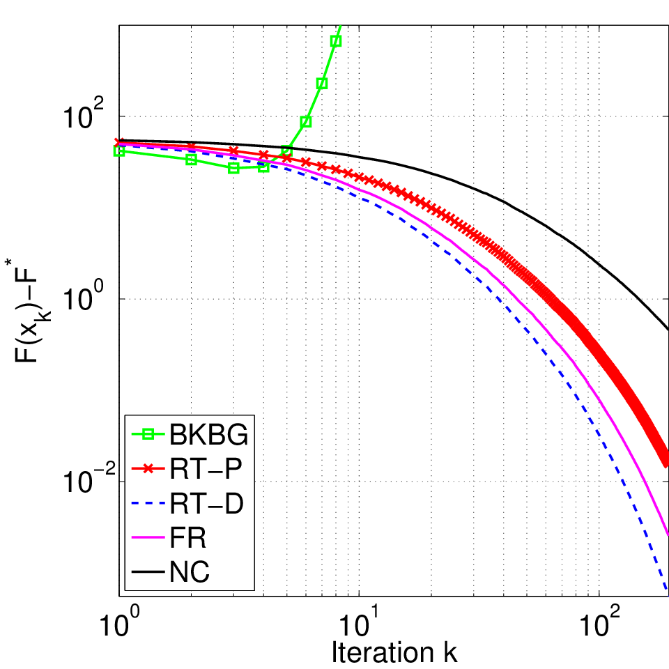
Parameter and hence for RT-P and for RT-D approach. The distribution of vectors can be found in Figure 1 (right). Figure 1 shows the evolution of for all 5 methods. Note that the BKBK did not converge. The speed of RT-P, RT-D and FR is quite similar and NC is approximately 3 times worse because .

SVM dual.
 |
 | |
 |
 |
In this experiment we compare 4 methods from Table 3 (we have excluded the naïve approach because it usually diverges for large ) on a real-world dataset astro-ph, which consists of data from papers in physics [29]. This dataset has training samples and a total of features. This dataset is very sparse. Indeed, each sample uses on average only features and each sample belongs to one of two classes. Hence, one might be interested in finding a hyperplane that separates the samples into their corresponding classes. The optimization problem can be formulated as follows:
| (65) |
where is the label of the class to which sample belongs.
While problem formulation (65) does not fit our framework (the nonsmooth part is nonseparable) the dual formulation (see [5, 30, 31]) does:
| (66) |
where . In particular, problem formulation (66) is the sum of a smooth term, and the restriction can be formulated as a (block separable) indicator function. In this dataset, each sample is normalized, hence .
For any dual feasible point we can obtain a primal feasible point . Moreover, from strong duality we know that if is an optimal solution of (66), then is optimal for problem (65). Therefore, we can associate a gap to each feasible point , which measures the distance of the objective value from optimality. Clearly .
Figure 2 (left) shows the evolution of as the iterates progress, and the distribution of ESO parameter for different choice of . Naturally, as increases, the distribution of shifts to the right, whereas the distribution of is not influenced by changing . The value of important parameters for other methods are and . For we have for RT-P and for RT-D approach and for we have for RT-P and for RT-D approach. Again the best performance is given by RT-D which requires knowledge of . If we do not want to estimate parameter then we should use FR. If was shown in [3] that for quadratic objective function FR is always better than RT-P.
References
- [1] Joseph K. Bradley, Aapo Kyrola, Danny Bickson, and Carlos Guestrin. Parallel coordinate descent for L1-regularized loss minimization. In 28th International Conference on Machine Learning, 2011.
- [2] Olivier Fercoq, Zheng Qu, Peter Richtárik, and Martin Takáč. Fast distributed coordinate descent for non-strongly convex losses. IEEE Workshop on Machine Learning for Signal Processing, 2014.
- [3] Olivier Fercoq and Peter Richtárik. Accelerated, Parallel and Proximal Coordinate Descent. arXiv:1312.5799, 2013.
- [4] Olivier Fercoq and Peter Richtárik. Smooth minimization of nonsmooth functions by parallel coordinate descent. arXiv:1309.5885, 2013.
- [5] Cho-Jui Hsieh, Kai-Wei Chang, Chih-Jen Lin, S Sathiya Keerthi, and S Sundararajan. A dual coordinate descent method for large-scale linear svm. In In ICML 2008, pages 408–415, 2008.
- [6] Martin Jaggi, Virginia Smith, Martin Takác, Jonathan Terhorst, Sanjay Krishnan, Thomas Hofmann, and Michael I Jordan. Communication-efficient distributed dual coordinate ascent. In Advances in Neural Information Processing Systems, pages 3068–3076, 2014.
- [7] Rie Johnson and Tong Zhang. Accelerating stochastic gradient descent using predictive variance reduction. In Advances in Neural Information Processing Systems, pages 315–323, 2013.
- [8] Jakub Konečný and Peter Richtárik. Semi-stochastic gradient descent methods. arXiv:1312.1666, 2013.
- [9] Yingying Li and Stanley Osher. Coordinate descent optimization for minimization with application to compressed sensing; a greedy algorithm. Inverse Problems and Imaging, 3(3):487–503, 2009.
- [10] Qihang Lin, Zhaosong Lu, and Lin Xiao. An accelerated proximal coordinate gradient method. In Advances in Neural Information Processing Systems, pages 3059–3067, 2014.
- [11] Ji Liu, Stephen J Wright, Christopher Ré, and Victor Bittorf. An asynchronous parallel stochastic coordinate descent algorithm. arXiv preprint arXiv:1311.1873, 2013.
- [12] Chenxin Ma, Virginia Smith, Martin Jaggi, Michael I Jordan, Peter Richtárik, and Martin Takáč. Adding vs. averaging in distributed primal-dual optimization. arXiv:1502.03508, 2015.
- [13] Mehrdad Mahdavi, Lijun Zhang, and Rong Jin. Mixed optimization for smooth functions. In Advances in Neural Information Processing Systems, pages 674–682, 2013.
- [14] Jakub Mareček, Peter Richtárik, and Martin Takáč. Distributed block coordinate descent for minimizing partially separable functions. arXiv:1406.0238, 2014.
- [15] Ion Necoara and Dragos Clipici. Distributed coordinate descent methods for composite minimization. arXiv:1312.5302, 2013.
- [16] Ion Necoara, Yurii Nesterov, and Francois Glineur. Efficiency of randomized coordinate descent methods on optimization problems with linearly coupled constraints. Technical report, 2012.
- [17] Yurii Nesterov. Gradient methods for minimizing composite objective function. CORE Discussion Paper 2007/76, 2007.
- [18] Yurii Nesterov. Efficiency of coordinate descent methods on huge-scale optimization problems. SIAM Journal on Optimization, 22(2):341–362, 2012.
- [19] Zheng Qu and Peter Richtárik. Coordinate descent with arbitrary sampling I: Algorithms and complexity. arXiv:1412.8060, 2014.
- [20] Zheng Qu and Peter Richtárik. Coordinate descent with arbitrary sampling II: Expected separable overapproximation. arXiv:1412.8063, 2014.
- [21] Zheng Qu, Peter Richtárik, and Tong Zhang. Randomized dual coordinate ascent with arbitrary sampling. arXiv:1411.5873, 2014.
- [22] Peter Richtárik and Martin Takáč. Efficient serial and parallel coordinate descent methods for huge-scale truss topology design. In Operations Research Proceedings 2011, pages 27–32. Springer Berlin Heidelberg, 2012.
- [23] Peter Richtárik and Martin Takáč. Distributed coordinate descent method for learning with big data. arXiv:1310.2059, 2013.
- [24] Peter Richtárik and Martin Takáč. On optimal probabilities in stochastic coordinate descent methods. arXiv:1310.3438, 2013.
- [25] Peter Richtárik and Martin Takáč. Iteration complexity of randomized block-coordinate descent methods for minimizing a composite function. Mathematical Programming Series A, pages 1–38, December 2012.
- [26] Peter Richtárik and Martin Takáč. Parallel coordinate descent methods for big data optimization. arXiv:1212.0873, 2012.
- [27] Ankan Saha and Ambuj Tewari. On the nonasymptotic convergence of cyclic coordinate descent methods. SIAM Journal on Optimization, 23(1):576–601, 2013.
- [28] Mark Schmidt and Michael Friedlander. Coordinate descent converges faster with the Gauss-Southwell rule than random selection. OPT-NIPS (Optimization workshop), 2014.
- [29] Shai Shalev-Shwartz, Yoram Singer, Nati Srebro, and Andrew Cotter. Pegasos: Primal Estimated sub-Gradient SOlver for SVM. Mathematical Programming: Series A and B- Special Issue on Optimization and Machine Learning, pages 3–30, 2011.
- [30] Shai Shalev-Shwartz and Tong Zhang. Stochastic dual coordinate ascent methods for regularized loss minimization. Journal of Machine Learning Research, 14:567–599, 2013.
- [31] Martin Takáč, Avleen Bijral, Peter Richtárik, and Nathan Srebro. Mini-batch primal and dual methods for SVMs. 30th International Conference on Machine Learning, 2013.
- [32] Q. Tao, K. Kong, D. Chu, and G. Wu. Stochastic coordinate descent methods for regularized smooth and nonsmooth losses. In P. A. Flach, T. De Bie, and N. Cristianini, editors, Machine Learning and Knowledge Discovery in Databases, volume 7523 of Lecture Notes in Computer Science, pages 537–552. Springer, 2012.
- [33] Rachael Tappenden, Peter Richtárik, and Jacek Gondzio. Inexact coordinate descent: Complexity and preconditioning. arXiv:1304.5530, 2013.
- [34] P. Tseng. Convergence of block coordinate descent method for nondifferentiable minimization. Journal of Optimization Theory and Applications, 109:475–494, June 2001.
- [35] P. Tseng and S. Yun. A coordinate gradient descent method for nonsmooth separable minimization. Math. Program., Ser. B, 117:387–423, 2009.
- [36] Stephen Wright. Accelerated block-coordinate relaxation for regularized optimization. SIAM Journal on Optimization, 22(1):159–186, 2012.
- [37] Stephen J Wright. Coordinate descent algorithms. optimization online 2014.12.4679, 2015.
- [38] Tong Tong Wu and Kenneth Lange. Coordinate descent algorithms for lasso penalized regression. Annals of Applied Statistics, 2(1):224–244, 2008.
- [39] Lin Xiao and Zhaosong Lu. On the complexity analysis of randomized block-coordinate descent methods. arXiv:1305.4723, 2013.
Appendix A Expected Separable Overapproximation
A.1 Smoothness assumptions
In this work we assume that the function is partially separable and smooth, and the purpose of this section is to define these two concepts. We begin with the definition of partial separability for a smooth convex function, introduced by Richtárik and Takáč in [26] .
Definition 13 (Partial separability [26]).
A smooth convex function is partially separable of degree if there exists a collection of subsets of such that
| (67) |
where for each , is a smooth convex function that depends on for only.
Now we introduce different types of smoothness assumptions for the function . Each smoothness type gives rise to a different ESO. Note that all of the following smoothness assumptions are equivalent. That is, if a given function satisfies one of the assumptions, then there exist constants such that the other assumptions also hold.
Assumption 14 ((Block) Coordinate-wise Lipschitz continuous gradient).
The gradient of is block Lipschitz, uniformly in , with positive constants . That is, for all , and we have
| (68) |
where denotes the gradient of and
| (69) |
The second type of assumption we make is that each function in the sum (67) has a Lipschitz continuous gradient. Such an assumption is made, for example, in [7, 8, 13, 15]. Moreover, we allow each function to have Lipschitz continuous gradient with a different constant (which was also assumed in [15]).
Assumption 15 (Lipschitz continuous gradient of sub-functions).
The gradient of has a Lipschitz continuous gradient, uniformly in , with positive constant with respect to some Euclidean norm . That is, for all , and we have
| (70) |
Note that this smoothness assumption is more general than that made in [15] because of the possibility of choosing general norms of the form . Further, Assumption 15 generalizes the smoothness assumptions imposed in [1, 23].
The third type of assumption we make is that each function in the sum (67) has coordinate-wise Lipschitz continuous gradient.
Assumption 16 ((Block) Coordinate-wise Lipschitz continuous gradient of sub-functions).
The gradient of is block Lipschitz, uniformly in , with non-negative constants . That is, for all , , and we have
| (71) |
One can think of Assumptions 14 and 15 as being ‘opposite’ to each other in the following sense. If we associate the block coordinates with the columns, and the functions with the rows, we see that Assumption 14 captures the dependence columns-wise, while Assumption 15 captures the dependence row-wise. Hence, Assumption 16 can be thought of as an element-wise smoothness assumption.
To make this more concrete, we present an example that demonstrates how to compute the Lipschitz constants for a quadratic function, under each of the three smoothness assumptions stated above.
Example 17.
Let the function , where and is th element of the matrix . Let us fix all the norms from Assumption 15 to be standard Euclidean norms. Then one can easily verify that equations (68), (70) and (71) are satisfied with the following choice of constants
In words, is equal to square of the norm of th column, is equal to the square of the norm of the th row and is simply the square of the th element of the matrix .
One could be misled into believing that Assumption 16 is the best because it is the most restrictive. However, while this is true for the quadratic objective shown in Example 17, for a general convex function, Assumption 16 can give Lipschitz constants that lead to worse ESO bounds (see Example 22 for further details).
A.2 Expected Separable Overapproximation (ESO)
Now, it is clear that the update in Algorithm 1 depends on the ESO parameter . This shows that the ESO is not just a technical tool; the parameters are actually used in Algorithm 1. Therefore we must be able to obtain/compute these parameters easily. We now present the following three theorems, namely Theorems 18, 20 and 21, that explain how to obtain the parameter for a -nice sampling, under different smoothness assumptions.
Theorem 18 (ESO for a -nice sampling, Theorem 14 in [26]).
Let Assumption 14 hold with constants and let be a -nice sampling. Then admits an ESO with respect to the sampling with parameter
where .
The obvious disadvantage of Theorem 18 is the fact that in the ESO, depends on . (When is large, so too is .) One can imagine a situation in which is much larger than the average cardinality of , resulting in a large . For example, if for is small for all but one function.
With this in mind, we introduce a new theorem that shows how the ESO in Theorem 18 can be modified if we know that Assumption 16 holds. In this case, the role of is slightly suppressed.
Theorem 19 (ESO for a doubly uniform sampling).
Let Assumption 16 hold with constants and let be a doubly uniform sampling. Then admits an ESO with respect to the sampling with parameter
| (72) |
Proof.
The following Theorem is a special case of Theorem 19 for a -nice sampling.
Theorem 20 (ESO for a -nice sampling, Theorem 1 in [3]).
Let Assumption 16 hold with constants and let be a -nice sampling. Then admits an ESO with respect to the sampling with parameter
| (73) |
Proof.
Notice that, if is -nice sampling, then and and the result follows from Theorem 19. ∎
The following theorem explains how to compute an ESO if Assumption 15 holds. This ESO was proposed and proved in [15].
Theorem 21 (ESO for -nice sampling, Lemma 1 in [15]).
Let Assumption 15 hold with constants and let be a -nice sampling. Then admits an ESO with respect to the sampling with parameter
where . Moreover, this ESO is monotonic.
As it is shown in Theorem 3 the speed of the algorithm (number of iterations needed to solve the problem) depends on ESO parameter via the term . Moreover, for a given objective function and sampling , there may be more than one ESO that could be chosen. Suppose that we have two ESOs to choose from, characterized by two parameters and respectively, and let . In this case, the ESO characterized by will give us (theoretically) faster convergence, and so it is obvious that this ESO should be used. Furthermore, is used as a parameter in Algorithm 1, and so, intuitively, this faster theoretical convergence, is expected to lead to fast practical performance.
In Section 6.1 in [3] it was shown that for a quadratic objective, the ESO in Theorem 18 is always worse than the ESO from Theorem 20. However, for a general objective the opposite can be true. The following simple example shows that the ESO from Theorems 20 and 21 can be times worse than the ESO from Theorem 18.
Example 22.
Remark. A thorough discussion of the ESO is presented in [26, Section 4]. Moreover, [26, Section 5.5] presents a list of parameters associated with a particular and sampling scheme that give rise to an ESO. Indeed, each of samplings described in Section 3.1 in this work gives rise to a for which an ESO exists.