Impact of size polydispersity on the nature of
Lennard-Jones liquids
Abstract
Polydisperse fluids are encountered everywhere in biological and industrial processes. These fluids naturally show a rich phenomenology exhibiting fractionation and shifts in critical point and freezing temperatures. Here, we study the impact of size polydispersity on the basic nature of Lennard-Jones (LJ) liquids, which represent most molecular liquids without hydrogen bonds, via two- and three-dimensional molecular dynamics computer simulations. A single-component liquid constituting spherical particles and interacting via the LJ potential is known to exhibit strong correlations between virial and potential energy equilibrium fluctuations at constant volume. This correlation significantly simplifies the physical description of the liquid, and these liquids are now known as Roskilde-simple (RS) liquids. We show that this simple nature of the single-component LJ liquid is preserved even for very high polydispersities (above 40% polydispersity for the studied uniform distribution). We also investigate isomorphs of moderately polydisperse LJ liquids. Isomorphs are curves in the phase diagram of RS liquids along which structure, dynamics, and some thermodynamic quantities are invariant in dimensionless units. We find that isomorphs are a good approximation even for polydisperse LJ liquids. The theory of isomorphs thus extends readily to multi-component systems and can be used to improve even further the understanding of these intriguing systems.
I Introduction
Polydisperse fluids are ubiquitous in both biological and industrial processes1, 2. Examples of polydisperse systems are: plastic materials, liquid foams, asphalt, micelles, and more. The property that typically varies among the constituent molecules is the charge, mass, and size. The fluids’ dispersity naturally induces a rich phenomenology not encountered in their single-component counterparts. As a consequence, polydisperse fluids have been the focus of a number of studies both theoretically 3, 4, 5, 6, 7, 8, 9, 10, 11 and via computer simulations 12, 13, 14, 15, 16, 17, 18, 19, 20, 21, 22, 23, 24, 11, 25, 26, 27, 28, 29, 30, 31, as well as in experiments 32, 33, 34, 35, 36, 37, 38, 39, 40.
These investigations revealed that polydisperse fluids exhibit a very rich phase diagram with shifts in critical point and freezing temperatures, as well as many-solid/fluid coexistence regions 41, 10. The coexisting phases in fact show fractionation, i.e., the dispersed variable displays a distribution different from the parent in each phase. Moreover, polydisperse fluids exhibit terminal polydispersity beyond which the solid is not stable 10, 25, 31. Polydispersity is thus regarded as an important factor to improve the glass-forming ability of liquids and to control the liquid fragility 42, 22, 36, 43, 23, 44.
Predicting the behavior of polydisperse fluids is a complex task, and several theoretical approaches have emerged to face the challenges of polydisperse fluids (see, e.g., Refs. 8, 9, 11, and 26). The complex nature of the problem is enhanced by the fact that quasi-universal relations45, 46, 47 for monatomic fluids, possessing great predictive power, break down in increasingly polydisperse fluids 48, 31. One such example is Rosenfeld’s excess entropy scaling45, 46 in which a dimensionless transport coefficient is correlated to the excess entropy with respect to an ideal gas. The latter observation for polydisperse fluids stands in contrast to confined fluids where the quasi-universal relations are very robust as the degree of confinement is increased 49, 50, 51, 52, 53.
Explanations for quasi-universal relations in monatomic fluids were recently presented from a constant-potential-energy NVU-dynamics perspective 54, 55, 56, 57, as well as from an exponential pair potential perspective 58, 59. In these perspectives, the quasi-universal relations are attributed to the monatomic fluids being so-called Roskilde-simple 60, 61, 62, 63, 64, 65, 66.
Roskilde-simple (RS) liquids have been detailed in a number of papers 60, 61, 62, 63, 64 and appear to be simpler than other types of liquids 66. RS liquids are characterized by having strong correlations between virial and potential energy equilibrium fluctuations at constant volume. In simulations of model liquids, the single-component Lennard-Jones (SCLJ) liquid, among many others, has been identified to belong to the class of RS liquids. Some experimental liquids have also been identified as RS 67, 68, 69. More specifically, the class of RS liquids is believed to include most or all van der Waals and metallic liquids, but to exclude most or all covalent-bonding, hydrogen-bonding, strongly ionic, and dipolar liquids60. Moreover, RS liquids are characterized by having isomorphs. Isomorphs are curves in the phase diagram of RS liquids along which structure, dynamics, and some thermodynamic quantities are invariant in dimensionless units; a property that is not limited to the stable liquid region but also valid in the supercooled liquid and even out-of-equilibrium63, 70.
Recently, Bagchi and coworkers25, 31 studied Lindemann’s melting and Hansen-Verlet’s freezing criterion in size polydisperse LJ liquids. The authors showed surprisingly that terminal polydispersity can be analyzed in terms of these rules. It was also shown that order-parameter maps for these liquids are not independent but highly correlated. We note that melting and freezing lines of RS liquids are isomorphs from which the rules of Lindemann and Hansen-Verlet follow63. In fact, correlated order-parameter maps also follow from the existence of isomorphs in the phase diagram63.
The observations of Bagchi and coworkers imply that polydisperse LJ liquids retain the character of RS liquids. Conversely, the breakdown of quasi-universal relations in polydisperse fluids may imply that polydisperse LJ liquids do not remain RS. Thus, we investigate in the following the effect of size polydispersity on strong virial-potential energy correlation in a systematic way to shed light on melting and freezing rules and quasi-universal behavior in polydisperse fluids. We note that previous investigations of multi-component RS liquids focused only on binary mixtures60, 64, 66.
Section II describes the applied methods and simulated model systems. Section III introduces RS liquids and explain their characteristics. In Sec. IV we show results from simulating size polydisperse LJ liquids in both two and three dimensions, in particular, the effect of size polydispersity on strong virial-potential energy correlation. Section V discusses the physics behind our observations. Finally, Sec. VI summarizes our work and presents an outlook.
II Simulation and model details
We apply NVT molecular dynamics computer simulations71, 72, 73 to study size polydisperse LJ liquids in two and three dimensions. The RUMD package (see http://rumd.org) is used for three-dimensional simulations while an in-house code is used for two-dimensional simulations. Pros and cons against applying constant-particle-number simulations to study polydisperse fluids are discussed in Ref. 74.
The polydisperse LJ liquid provides a convenient framework for initiating theoretical investigations of polydispersity18, 31, but has also been applied to mimic the behavior of for instance hydrocarbon or polymer solutions, idealized models for spherical micelles in water above the critical micelle concentration, and polystyrene lattices stabilized with polyoxyethylene chains41.
If the total potential energy of the system is given by = , the size polydisperse LJ pair potential is
| (1) |
where and set, respectively, the length and energy scale of the pair interaction between particle and particle (, in which is the number of particles). As the study is focused on size polydisperse LJ liquids: is independent of the pair interaction and fixed in simulations. The parameter is defined from the Lorentz-Berthelot mixing rule75 given by
| (2) |
In this study, and are evenly distributed on an interval from to . The polydispersity of the liquid is defined by
| (3) |
where and are, respectively, the dispersed variable’s standard deviation and mean. We study polydispersities in the range = 0% to = 52% and apply a truncated-and-shifted pair potential cutoff at . We note that care should be taken when comparing the absolute polydispersity number amongst different distributions18.
The units of the simulation are defined by setting the mean values
over the particles to unity, i.e., , , = 1.
All particle masses are identical (and equal to unity).
Figure 1 shows pair potentials of Eq. (1) with
= 0.1, 1.0, 1.9 and = 1. The latter
corresponds to the range of LJ potentials used
in simulations of a size polydisperse LJ liquid with = 52% (i.e., = 0.1 and = 1.9). For this high polydispersity the simulated pair potentials cover a very broad range of potentials.

The two-dimensional simulations use = 1000 particles, whereas the three-dimensional simulations use particles. The finite-size effects are larger in two dimensions than in three dimensions. In either case, however, finite-size effects are observed to be small for the quantities studied in this paper and no additional averaging is performed.
III Roskilde-simple liquids
RS liquids and their associated simple properties have been detailed in a number of papers, starting with a series of five papers60, 61, 62, 63, 64. RS liquids are characterized by having strong correlations between virial and potential energy equilibrium fluctuations at constant volume. The virial-potential energy correlation is quantified via Pearson’s correlation coefficient given by
| (4) |
in which is deviation from mean values, denotes NVT ensemble averages, and . RS liquids are defined pragmatically by requiring . depends on the state point investigated but has been shown to be high in large parts of the phase diagram or not at all.
Only inverse power-law (IPL) fluids with pair potentials are perfectly correlating ( = 1 since ), but many models60, 66, 76, such as the SCLJ liquid, the Kob-Andersen binary LJ mixture, the Lewis-Wahnström OTP model, the asymmetric dumbbell model, identical chain length LJ-bead polymer models, and some experimental liquids67, 68, 69, have been shown to belong to the class of RS liquids.
The origin behind strong correlation in the SCLJ liquid is as follows. The LJ pair potential can be approximated by an IPL potential in the repulsive part77, 78, 79, i.e., below the potential mininum with an IPL-exponent . The required exponent is larger than the repulsive term encountered in the LJ potential as the effect of attraction is to increase the steepness of the repulsive part. However, contributions to the fluctuations come from pair distances around the pair potential minimum61, 66. As a consequence, one must add a linear term and a constant to the IPL potential to obtain a proper description of the LJ potential:
| (5) |
The constraint of constant volume in the NVT ensemble has the following effect: When one nearest-neighbor distance increases another one decreases. Thus, upon summation the contribution from the linear term to and is almost constant and vanishes with respect to the fluctuations. For a very recent review of RS liquids, see Ref. 80.
As mentioned, RS liquids are associated with a number of simple properties. RS liquids are, for instance, characterized by having isomorphs to a good approximation63. Consider two state points in a liquid’s phase diagram with density and temperature (, ) and (, ). These two state points are defined to be isomorphic if the following holds: Whenever a microconfiguration of state point () and of state point () have the same reduced coordinates, = (R denotes a 3-dimensional configurational-space vector and , in which is the volume), these two configurations have proportional Boltzmann factors, i.e.,
| (6) |
Here is a constant and depends only on the state points () and (). An isomorph is defined as a continuous curve of state points that are all pairwise isomorphic. For IPL fluids = 1, and isomorphs thus encapsulate the well-known scaling properties81 of these systems. However, for all other RS liquids ; accordingly, the state points can be represented effectively on a one-dimensional phase diagram only for certain properties 63.
An immediate consequence of isomorphs is that a number of quantities are invariant along these curves. The invariants include the structure and dynamics in reduced units and some thermodynamic quantities, e.g., the excess entropy with respect to an ideal gas . We note that reduced units refer to macroscopic quantities, such as and , rather than the usual approach in simulations via microscopic quantities (see Ref. 63 for details).
For RS liquids, temperature separates65 in a function of density and of excess entropy: . From this equation, one observes the isomorph invariant which was used to define the so-called isomorph scaling65, 82, in which the reduced relaxation time is a function = . Isomorph scaling explains classical density scaling83 for which , where is a fitting exponent. Density scaling is valid only for relatively small density variations, whereas isomorph scaling works even when the density variation is large82. Additionally, the isomorph invariant provides a convenient way to generate isomorphs since inherits the analytical structure of the potential energy function65.
There exist additional simple observations for RS liquids than mentioned so far, e.g., the dominance of first-coordination shell interactions66, 84, extension to non-trivial boundary conditions such as nanoconfinement52 or shear-flow70, crystalline isomorphs85, and the relevance of Rosenfeld-Tarazona’s expressions86 for these liquids87. The interested reader is referred to these and other papers for more information.
Finally, a reformulation of isomorphs was very recently presented88. If and denote two different 3-dimensional configurational-space vectors of a chosen state point, the isomorphic condition is
| (7) |
where is a scalar. This definition encapsulates the previous definition of isomorphs as a (very good) first-order approximation88. The mentioned invariants are exact within this reformulation, too. We note, however, that the constant volume heat capacity is not formally invariant.
IV Results from polydisperse LJ liquids
The simulations in this paper were performed both in two and three dimensions, and thus we discuss each case separately beginning with the two-dimensional results.
IV.1 Simulations in two dimensions
The investigation is initiated by considering the effect of size polydispersity on the structure and dynamics of the SCLJ liquid in two dimensions at = 0.75 and = 0.70. For 0% polydispersity, this state point corresponds to the liquid phase.
Figure 2(a) presents radial distribution functions (RDFs) upon the increase of polydispersity from = 0% to = 52%, whereas Fig. 2(b) shows bond-orientational-order functions89, 22 (BOFs) defined via
| (8) |
The division with in Fig. 2(b) approximately accounts for effects due to positional order in the liquid90, 22. In the equation above, denotes Dirac’s -function, , is the box length, and , in which is the number of nearest neighbors of particle , and is the angle between the vector and the -axis (particle is a neighbor of particle ). Nearest-neighbor particles are identified via a Voronoi-construction75. Finally, Fig. 2(c) shows mean-square displacements (MSDs).
Both measures of structural order (Figs. 2(a) and (b)) are seen to vanish as polydispersity is increased from = 0% to = 52% at constant density and temperature.
The MSD shows approximately one order-of-magnitude decrease in the
diffusion coefficient over the same variation in
polydispersity. Introducing size polydispersity has thus a pronounced effect on the SCLJ liquid. The latter results confirm several previous simulations of polydisperse hard-sphere and LJ
liquids12, 18, 25. We note that if the volume (area) fraction of the system is
kept constant, instead of density, a similar diminishment of structural
correlations is observed. However, in the case of the dynamics an enhancement of the mobility is seen23.
![[Uncaptioned image]](1503.02866v1/rdf_075.png)
![[Uncaptioned image]](1503.02866v1/rdf6.png)

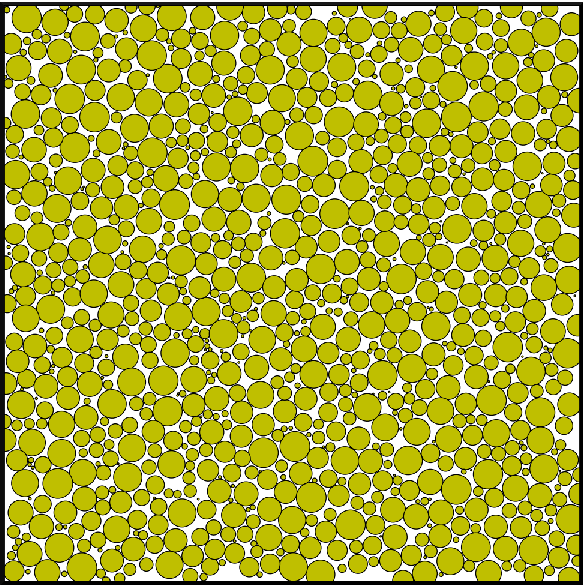
Furthermore, Fig. 3 shows a snapshot of a particle configuration for the size polydisperse
LJ liquid with = 0.75, = 0.70, = 52%. Each particle is represented according to its value of . A multitude of
different sizes are present at this high polydispersity exemplifying again
the rich and non-trivial diversity of the liquids studied.
The study is now turned towards the assessment of the effect of size polydispersity from the viewpoint of RS liquids. In this connection, we note that previous simulations of RS liquids were performed only in three dimensions. The simulations in this section are two-dimensional.
Figure 4 shows the correlation coefficient as function of polydispersity at both
constant density (black data points) and constant
volume fraction (red data points). For the three-dimensional SCLJ liquid, a typical value for the correlation coefficient is .
The inset shows the density-scaling exponent63, 65 as function of
polydispersity (see Sec. III).

At constant density, we observe both a decrease and an increase in depending on the starting state point at 0% polydispersity. This observation is expected as the phase diagram for polydisperse liquids shows very rich phenomenology41, 10. Although a decrease in is observed for the two highest densities ( = 0.95 and = 0.85) all state points investigated are RS. For the lowest density ( = 0.75) the liquid becomes RS at high polydispersities. In fact, the results show that polydisperse LJ liquids at 52% polydispersity are RS liquids. This observation is non-trivial given the complex nature of polydisperse liquids (see also Fig. 3).
In the case of constant volume fraction, however, we observe a significant decrease in as function of polydispersity. An increase in polydispersity, at constant volume fraction, is accompanied by a decrease in pressure. This is in contrast to constant density which increases the pressure; Table 1 shows selected polydispersities and corresponding volume fractions along the three simulated constant-density curves. For the density-scaling exponent , we only observe a decrease in its value, when polydispersity is increased.
| ( = 0.75) | ( = 0.85) | ( = 0.95) | |
|---|---|---|---|
| 0 | 0.589 | 0.668 | 0.746 |
| 11.55 | 0.597 | 0.676 | 0.755 |
| 23.09 | 0.619 | 0.702 | 0.784 |
| 34.64 | - | 0.746 | 0.834 |
| 51.96 | 0.746 | 0.845 | - |
As mentioned previously, the quantity is invariant along an isomorph (see Sec. III). The function for a LJ liquid in two dimensions is given by
| (9) |
In the equation above: , is a chosen reference density, and is the value of = obtained from the equilibrium fluctuations at (see Refs. 65 and 82 for additional details). In this and the following section the reference state point is = 1 and = 1. We now proceed to study isomorphs of a moderately polydisperse LJ liquid. Isomorphs are generated by the procedure stated below65, 82:
- 1.
A starting state point is chosen.
- 2.
Density is varied by some percentage (typically 10-20% but can be even a factor of two82).
- 3.
The temperature of the isomorphic state point is calculated via Eq. (9) keeping constant.
- 4.
A simulation is performed at the predicted state point and the procedure is repeated.
Figure 5(a) shows RDFs along an isomorph with 20% density
increase ( = 7.02 and starting state point = 0.85 and = 0.70). For
reference, Fig. 5(b) shows an isotherm with the same density increase. A good invariance of structure is seen along the isomorph, whereas
structure on the isotherm clearly shows a poorer scaling.
![[Uncaptioned image]](1503.02866v1/isomorph_rdf.png)

Figure 6 shows the corresponding BOF figures. A good invariance is again seen along the isomorph but not
along the isotherm.
![[Uncaptioned image]](1503.02866v1/isomorph_rdf6.png)

Turning to the dynamics in Fig. 7, a near-perfect collapse is seen for the MSD on the isomorph whereas, as expected, a poor invariance is seen along the isotherm.
The fact that liquids are highly size polydisperse is thus not a hindrance to showing simple isomorphic behavior.
![[Uncaptioned image]](1503.02866v1/isomorph_msd.png)

IV.2 Simulations in three dimensions
This section studies size polydisperse LJ liquids in three dimensions. Figure 8 shows the correlation coefficient
as function of polydispersity at constant density and volume fraction. As for the two-dimensional
results both a decrease and an increase in is observed, when
polydispersity is increased at constant density (i.e., increasing pressure). For the density = 0.75, the liquid becomes RS at high polydispersities, whereas for
= 0.85 and = 0.97 all state points investigated are RS, albeit decreases. We observe again that highly size polydisperse LJ liquids are RS: a non-trivial observation.

In the case of constant volume fraction, a significant decrease in is observed and is accompanied by the virial turning negative (but not the pressure). Actually, the liquid goes from RS to non-RS in the studied range of polydispersities. For single-component liquids: usually decreases rapidly, when the virial becomes negative60.
The density-scaling exponent shows as in two dimensions a decrease in its value as function of polydispersity. Actually, it is observed from Fig. 8 that all constant-density curves collapse at high polydispersities with 4.5. Even a path at = 52%, where density varies from = 0.97 to 0.60 ( = 0.94 to 0.58) and the virial from = 110 to 5.8, gives approximately the same value of (see magenta asteriks data points).
This observation indicates that for highly size polydisperse LJ liquids is mainly controlled by the degree of polydispersity . In the non-reformulated isomorph theory is predicted to be a function only of density65 (see Sec. III). For the SCLJ liquid, a value of 5.5 is obtained at low-to-moderate pressures (see inset and Ref. 65).
Very recently, an expression was established relating to the pair potential of monatomic RS liquids91. The expression is given by
| (10) | ||||
| (11) |
where is a dimensionless number, and is the ’th derivative of the pair potential . is then related to the curvature and torsion of the pair potential. is chosen as the reduced distance ( = at which obtains its maximum, i.e., the most likely nearest-neighbor distance91. In this case, however, is not a function only of density.
RDFs along an isomorph and isotherm for a polydisperse LJ liquid with = 23.09% are given in Fig. 9 ( = 4.79 and starting state point = 0.97 and = 0.70). The isomorph is generated via the aforementioned procedure keeping constant. The expression65 for in three dimensions is given by
| (12) |
with definitions provided in the previous section. The RDF is to a good approximation invariant along the isomorph and less so on the
isotherm (the highest density state point is, however, not fully equilibrated due to slow dynamics).
![[Uncaptioned image]](1503.02866v1/3D_rdf_isomorph.png)

Figure 10 shows BOFs along the same isomorph and isotherm. The BOF is defined in three dimensions via
| (13) |
in which
| (14) | ||||
| (15) |
The above expression for gives coarse-grained Steinhardt bond-orientational-order parameters90, 92.
is the spherical harmonic function with degree = 6 and order = . The notation indicates that the sum is
taken over all the nearest neighbors of particle including particle itself; nearest-neighbor particles are identified via
the twelve-closest particles. From Fig. 10, a similar conclusion as for the RDF is reached; a good invariance is observed along the isomorph and less so on the isotherm.
These results also indicate a good invariance of the first coordination shell (FCS) environment along the isomorph and are consistent with the role
of the FCS in determining the structure and dynamics of RS liquids (see Ref. 66 for more information on FCS results).
![[Uncaptioned image]](1503.02866v1/3D_rdf6_isomorph.png)

Finally, the dynamics in terms of the MSD is shown in Fig. 11. An excellent invariance is obtained along the isomorph, whereas the
isotherm shows approximately five orders-of-magnitude reduction in the diffusion coefficient.
![[Uncaptioned image]](1503.02866v1/3D_msd_isomorph.png)

V Discussion
We have demonstrated that both two- and three-dimensional size polydisperse LJ liquids belong to the class of RS liquids up to a significant level of polydispersity. This shows that the theory of isomorphs can be applied to multi-component systems which contributes to the simpler physical description of this important class of liquids. Nevertheless, our simulations also showed unusual behavior when compared to the SCLJ liquid. 1) At higher densities, decreased with increasing polydispersity (pressure). An increase in pressure normally reduces interparticle distances in which a pure IPL description is a better approximation, and one would a priori expect to increase. 2) For high polydispersities, the density-scaling exponent is controlled only by the degree of polydispersity exhibiting also significantly lower -values at low-to-moderate pressures ( versus 5.5 in three dimensions). Below we try to understand these observations in more detail presenting three-dimensional results only.
Figure 12 shows like-like RDFs (colored curves) for the small, medium, and large particles at = 0.85, = 0.70, = 52%, and the corresponding SCLJ liquid RDF (black curve). The RDFs for the medium and large particles move to shorter distances when compared to the SCLJ liquid (note the scaled distance axis). Conversely, the RDF for the small particles moves to larger distances and shows a very broad distribution. The higher value of the first peak is due to a clustering tendency of small particles in spaces surrounded by bigger particles (see Fig. 3)
The results signify a decoupling, with respect to pressure, amongst the small and large particles and could be the reason why decreases with increasing polydispersity (pressure) at higher densities. To verify this, we simulated at the same state point (not shown) a truncated uniform distribution excluding all the small(er) particles (i.e., particles with ). In this case: increased with polydispersity (pressure).
Despite that the small particles are located around the minimum of the LJ potential, fluctuations
in their positions are quite large. We speculate that this large-amplitude positional fluctuation
might diminish the impact of the particle-size dependent inhomogeneous stress distribution on (see Eq. (5)).
Accordingly, it may also explain why the liquid remains RS up to such high polydispersities.
Additional studies are, however, needed to clarify this issue.

The investigation is now focused on -values at low-to-moderate pressures for high polydispersities (). In the light of the theoretical results on monatomic RS liquids (see Eq. (10)), Fig. 13(a) shows for the small (), medium (), and large () particles ( = , , ) at = 0.60, = 0.70, = 52% ( = 5.8). Figure 13(b) shows for the LJ potential (Eq. (11)). Disregarding now the fact that the liquid is polydisperse we apply to make predictions for using the procedure mentioned in Sec. IV.2 for RS monatomic liquids.
In this way 5.5 and 4.9 are obtained for the medium
and large particles, respectively, whereas gives a negative value due to
the divergence in . Interestingly, gives a value very close to that expected for a SCLJ liquid at low-to-moderate pressures ( 5.5).
Nevertheless, the results indicate that the large particles play an important role in determining the value of for polydisperse LJ liquids with 4.9.
It is, however, unclear which role the small particles play, as peaks at very large
distances with a resulting negative .
We speculate that there is some cancellation between the medium particles of large and the small particles of negative .
More in-depth investigations are, however, needed.
![[Uncaptioned image]](1503.02866v1/most_likely.png)

VI Conclusion and outlook
Polydisperse fluids show rich phenomenology with respect to their single-component fluid counterparts and manifest themselves in as diverse systems as bitumen in road construction93 to micelles in biological systems41. In spite of this fact, we have shown that even highly size polydisperse LJ liquids belong to the class of RS liquids. As a consequence, polydisperse LJ liquids inherit the associated simple properties of RS liquids66, 63 and are exemplified here by studying isomorphs of moderately polydisperse LJ liquids in both two and three dimensions.
The SCLJ liquid is a prime example of a RS liquid, however, many more model and experimental liquids are identified to belong to this class of liquids. A natural question thus arises: How are the remaining RS liquids affected by introducing size polydispersity? As an example, identical chain length LJ-bead polymer models have very recently been identified as RS76. For polymers the relevant size polydispersity is given by a distribution of chain lengths (mass distribution); can one expect such polymeric liquids to be RS? The answer is most likely in the affirmative. It is known from experiments that scaling relations typical of RS liquids, such as density scaling and excess entropy scaling, are also valid for polymers83. As another example, rigid-bond molecular liquids with LJ interactions have also been identified as RS94; it is expected that these liquids remain RS when introducing size polydispersity. A more general hypothesis is that all RS liquids will remain so to a high degree of accuracy when introducing size polydispersity. Future research should, however, focus on clarifying to what extent this hypothesis is valid and on understanding the implications thereof.
To conclude, the theory of isomorphs extends readily to multi-component systems, and when doing so it can be applied to improve even further the understanding of these intriguing systems. Experimental liquids are often distributed in additional or other variables such as mass or charge41, 7, 18. More work in this direction is also needed to understand how these factors influence the results presented here.
Acknowledgements.
Valuable discussions with Lorentzo Costigliola, Jeppe C. Dyre, Claire Lemarchand, and Thomas B. Schrøder are gratefully acknowledged. This work was partially supported by Grant-in-Aid for Scientific Research (S) and Specially Promoted Research from the Japan Society for the Promotion of Science (JSPS). T.S.I. acknowledges support from a JSPS Postdoctoral Fellowship.References
- [1] Bagchi, B. Molecular Relaxation in Liquids; Oxford University Press: New York, 2012.
- [2] Wolynes, P. G., Lubchenko, V., Eds. Structural Glasses and Supercooled Liquids: Theory, Experiment, and Applications; John Wiley and Sons, Inc., 2012.
- [3] Dickinson, E. Chem. Phys. Lett. 1978, 57, 148.
- [4] Blum, L.; Stell, G. J. Chem. Phys. 1979, 71, 42.
- [5] Salacuse, J. J.; Stell, G. J. Chem. Phys. 1982, 77, 3714.
- [6] Gualtieri, J. A.; Kincaid, J. M.; Morrison, G. J. Chem. Phys. 1982, 77, 521.
- [7] Ginoza, M.; Yasutomi, M. Mol. Phys. 1997, 91, 59.
- [8] Evans, R. M. L. Phys. Rev. E 1999, 59, 3192.
- [9] Sollich, P. J. Phys.: Condens. Matter 2002, 14, R79.
- [10] Fasolo, M.; Sollich, P. Phys. Rev. Lett. 2003, 91, 068301.
- [11] Jacobs, W. M.; Frenkel, D. J. Chem. Phys. 2013, 139, 024108.
- [12] Frenkel, D.; Vos, R. J.; de Kruif, C. G.; Vrij, A. J. Chem. Phys. 1986, 84, 4625.
- [13] Kofke, D. A.; Glandt, E. D. FFE 1986, 29, 327.
- [14] Kofke, D. A.; Glandt, E. D. J. Chem. Phys. 1987, 87, 4881.
- [15] Stapleton, M. R.; Tildesley, D. J.; Quirke, N. J. Chem. Phys. 1990, 92, 4456.
- [16] Auer, S.; Frenkel, D. Nature 2001, 413, 711.
- [17] Kristóf, T.; Liszi, J. Mol. Phys. 2001, 99, 167.
- [18] Murarka, R. K.; Bagchi, B. Phys. Rev. E 2003, 67, 051504.
- [19] Wilding, N. B.; Sollich, P. J. Phys.: Condens. Matter 2005, 17, S3245.
- [20] Wilding, N. B.; Sollich, P.; Fasolo, M. Phys. Rev. Lett. 2005, 95, 155701.
- [21] Wilding, N. B.; Sollich, P.; Fasolo, M.; Buzzacchi, M. J. Chem. Phys. 2006, 125, 014908.
- [22] Kawasaki, T.; Araki, T.; Tanaka, H. Phys. Rev. Lett. 2007, 99, 215701.
- [23] Abraham, S. E.; Bhattacharrya, S. M.; Bagchi, B. Phys. Rev. Lett. 2008, 100, 167801.
- [24] W.-S. Xu, Z.-Y. S.; An, L.-J. Phys. Rev. E 2012, 86, 041506.
- [25] Sarkar, S.; Biswas, R.; Santra, M.; Bagchi, B. Phys. Rev. E 2013, 88, 022104.
- [26] Ogarko, V.; Luding, S. Soft Matter 2013, 9, 9530.
- [27] Williamson, J. J.; Evans, R. M. L. Soft Matter 2013, 9, 3600.
- [28] Ashton, D. J.; Jack, R. L.; Wilding, N. B. Soft Matter 2013, 9, 9661.
- [29] Nguyen, D.-H.; Azéma, E.; Radjai, F.; Sornay, P. Phys. Rev. E 2014, 90, 012202.
- [30] Phillips, C. L.; Glotzer, S. C. J. Chem. Phys. 2014, 137, 104901.
- [31] Sarkar, S.; Biswas, R.; Ray, P. P.; Bagchi, B. arXiv 2014, 1402.6879.
- [32] Koningsveld, R.; Kleintjens, L. A. Macromolecules 1971, 4, 637.
- [33] Cowell, C.; Vincent, B. J. Colloid Interface Sci. 1982, 87, 518.
- [34] Weeks, E. R.; Crocker, J. C.; Levitt, A. C.; Schofield, A.; Weitz, D. A. Science 2000, 287, 627.
- [35] Ye, X.; Sridhar, T. Macromolecules 2005, 38, 3442.
- [36] Watanabe, K.; Tanaka, H. Phys. Rev. Lett. 2008, 100, 158002.
- [37] Ballesta, P.; Duri, A.; Cipelletti, L. Nat. Phys. 2008, 4, 550.
- [38] Banerjee, S.; Ghosh, R.; Bagchi, B. J. Phys. Chem. B 2012, 116, 3713.
- [39] Sacanna, S.; Korpics, M.; Rodriguez, K.; Colón-Meléndez, L.; Kim, S.-H.; Pine, D. J.; Yi, G.-R. Nat. Commun. 2013, 4, 1688.
- [40] Palberg, T. J. Phys.: Condens. Matter 2014, 26, 333101.
- [41] Stapleton, M. R.; Tildesley, D. J.; Sluckin, T. J.; N, Q. J. Phys. Chem. 1988, 92, 4788.
- [42] Tanaka, H. Eur. Phys. J. E 2012, 35, 113.
- [43] Tanaka, H.; Kawasaki, T.; Shintani, H.; Watanabe, K. Nat. Mater. 2010, 9, 324.
- [44] Abraham, S. E.; Bagchi, B. Phys. Rev. E 2008, 78, 051501.
- [45] Rosenfeld, Y. Phys. Rev. A 1977, 15, 2545.
- [46] Rosenfeld, Y. J. Phys.: Condens. Matter 1999, 11, 5415.
- [47] Dzugutov, M. Nature 1996, 381, 137.
- [48] Pond, M. J.; Errington, J. R.; Truskett, T. M. J. Chem. Phys. 2011, 135, 124513.
- [49] Mittal, J.; Errington, J. R.; Truskett, T. M. Phys. Rev. Lett. 2006, 96, 177804.
- [50] Mittal, J.; Errington, J. R.; Truskett, T. M. J. Phys. Chem. B 2007, 111, 10054.
- [51] Watanabe, K.; Kawasaki, T.; Tanaka, H. Nat. Mater. 2011, 10, 512.
- [52] Ingebrigtsen, T. S.; Errington, J. R.; Truskett, T. M.; Dyre, J. C. Phys. Rev. Lett. 2013, 111, 235901.
- [53] Hanakata, P. Z.; Douglas, J. F.; Starr, F. W. Nat. Commun. 2014, 5, 4163.
- [54] Dyre, J. C. Phys. Rev. E 2013, 87, 022106.
- [55] Ingebrigtsen, T. S.; Toxvaerd, S.; Heilmann, O. J.; Schrøder, T. B.; Dyre, J. C. J. Chem. Phys. 2011, 135, 104101.
- [56] Ingebrigtsen, T. S.; Toxvaerd, S.; Schrøder, T. B.; Dyre, J. C. J. Chem. Phys. 2011, 135, 104102.
- [57] Ingebrigtsen, T. S.; Dyre, J. C. J. Chem. Phys. 2012, 137, 244101.
- [58] Bacher, A. K.; Dyre, J. C. Colloid. Polym. Sci. 2014, 292, 1971.
- [59] Bacher, A. K.; Schrøder, T. B.; Dyre, J. C. Nat. Commun. 2014, 5, 5424.
- [60] Bailey, N. P.; Pedersen, U. R.; Gnan, N.; Schrøder, T. B.; Dyre, J. C. J. Chem. Phys. 2008, 129, 184507.
- [61] Bailey, N. P.; Pedersen, U. R.; Gnan, N.; Schrøder, T. B.; Dyre, J. C. J. Chem. Phys. 2008, 129, 184508.
- [62] Schrøder, T. B.; Bailey, N. P.; Pedersen, U. R.; Gnan, N.; Dyre, J. C. J. Chem. Phys. 2009, 131, 234503.
- [63] Gnan, N.; Schrøder, T. B.; Pedersen, U. R.; Bailey, N. P.; Dyre, J. C. J. Chem. Phys. 2009, 131, 234504.
- [64] Schrøder, T. B.; Gnan, N.; Pedersen, U. R.; Bailey, N. P.; Dyre, J. C. J. Chem. Phys. 2011, 134, 164505.
- [65] Ingebrigtsen, T. S.; Bøhling, L.; Schrøder, T. B.; Dyre, J. C. J. Chem. Phys. 2012, 136, 061102.
- [66] Ingebrigtsen, T. S.; Schrøder, T. B.; Dyre, J. C. Phys. Rev. X 2012, 2, 011011.
- [67] Gundermann, D.; Pedersen, U. R.; Hecksher, T.; Bailey, N. P.; Jakobsen, B.; Christensen, T.; Olsen, N. B.; Schrøder, T. B.; Fragiadakis, D.; Casalini, R.; Roland, C. M.; Dyre, J. C.; Niss, K. Nat. Phys. 2011, 7, 816.
- [68] Roed, L. A.; Gundermann, D.; Dyre, J. C.; Niss, K. J. Chem. Phys. 2013, 139, 101101.
- [69] Xiao, W.; Tofteskov, J.; Christensen, T. V.; Dyre, J. C.; Niss, K. J. Non-Crystal. Solids 2014, http://dx.doi.org/10.1016/j.jnoncrysol.2014.08.041.
- [70] Separdar, L.; Bailey, N. P.; Schrøder, T. B.; Davatolhagh, S.; Dyre, J. C. J. Chem. Phys. 2013, 138, 154505.
- [71] Nosé, S. J. Chem. Phys. 1984, 81, 511.
- [72] Hoover, W. G. Phys. Rev. A 1985, 31, 1695.
- [73] Toxvaerd, S. Mol. Phys. 1991, 72, 159.
- [74] Wilding, N. B.; Sollich, P. J. Chem. Phys. 2010, 133, 224102.
- [75] Allen, M. P.; Tildesley, D. J. Computer Simulation of Liquids; Oxford University Press: New York, 1987.
- [76] Veldhorst, A. A.; Dyre, J. C.; Schrøder, T. B. J. Chem. Phys 2014, 141, 054904.
- [77] Coslovich, D.; Roland, C. M. J. Phys. Chem. B 2008, 112, 1329.
- [78] Coslovich, D.; Roland, C. M. J. Chem. Phys. 2009, 130, 014508.
- [79] Coslovich, D.; Roland, C. M. J. Chem. Phys. 2009, 131, 151103.
- [80] Dyre, J. C. J. Phys. Chem. B 2014, 118, 10007.
- [81] Hoover, W. G.; Ross, M.; Johnson, K. W.; Henderson, D.; Barker, J. A.; Brown, B. C. J. Chem. Phys. 1970, 52, 4931.
- [82] Bøhling, L.; Ingebrigtsen, T. S.; Grzybowski, A.; Paluch, M.; Dyre, J. C.; Schrøder, T. B. New J. Phys. 2012, 14, 113035.
- [83] Roland, C. M. Macromolecules 2010, 43, 7875.
- [84] Ingebrigtsen, T. S.; Dyre, J. C. Soft Matter 2014, 10, 4324.
- [85] Albrechtsen, D. E.; Olsen, A. E.; Pedersen, U. R.; Schrøder, T. B.; Dyre, J. C. Phys. Rev. B 2014, 90, 094106.
- [86] Rosenfeld, Y.; Tarazona, P. Mol. Phys. 1998, 95, 141.
- [87] Ingebrigtsen, T. S.; Veldhorst, A. A.; Schrøder, T. B.; Dyre, J. C. J. Chem. Phys. 2013, 139, 171101.
- [88] Schrøder, T. B.; Dyre, J. C. J. Chem. Phys. 2014, 141, 204502.
- [89] Binder, K.; Sengupta, S.; Nielaba, P. J. Phys.: Condens. Matter 2002, 14, 2323.
- [90] Steinhardt, P. J.; Nelson, D. R.; Ronchetti, M. Phys. Rev. B 1983, 28, 784.
- [91] Bøhling, L.; Bailey, N. P.; Schrøder, T. B.; Dyre, J. C. J. Chem. Phys. 2014, 140, 124510.
- [92] Lechner, W.; Dellago, C. J. Chem. Phys. 2008, 129, 114707.
- [93] Hansen, J. S.; Lemarchand, C. A.; Nielsen, E.; Dyre, J. C.; Schrøder, T. J. Chem. Phys. 2013, 138, 094508.
- [94] Ingebrigtsen, T. S.; Schrøder, T. B.; Dyre, J. C. J. Phys. Chem. B 2012, 116, 1018.