Free Space Optical Communication with Spatial Modulation and Coherent Detection over H-K Atmospheric Turbulence Channels
Abstract
The use of optical spatial modulation (OSM), which has been recently emerged as a power and bandwidth efficient pulsed modulation technique for indoor optical wireless communication, is proposed as a simple, low-complexity means of achieving spatial diversity in coherent free space optical (FSO) communication systems. In doing so, this paper makes several novel contributions as follows. It presents a generic analytical framework for obtaining the Average Bit Error Probability (ABEP) of uncoded OSM with coherent detection in the presence of turbulence-induced fading. Although the framework is general enough to accommodate any type of models based on turbulence scattering, the focus in this paper is the H-K distribution. Although this distribution represents a very general scattering model valid over a wide range of atmospheric conditions, it is has not been considered in the past in conjunction with FSO systems possibly because of its mathematical complexity. The proposed analytical framework yields exact performance evaluation results for MIMO systems with two transmit– and an arbitrary number of receive apertures. In addition, tight upper bounds are derived for the error probability for OSM systems with an arbitrary number of transmit apertures as well as for convolutionally encoded signals. The performance of OSM is compared to that of well established coherent FSO schemes, employing spatial diversity at the transmitter or the receiver only. Specifically, it is shown that OSM can offer comparable performance with conventional coherent FSO schemes while outperforming the latter in terms of spectral efficiency and hardware complexity. Various numerical performance evaluation results are also presented and compared with equivalent results obtained by Monte Carlo simulations which verify the accuracy of the derived analytical expressions.
Index Terms:
average bit error probability, atmospheric turbulence, coherent detection, free space optical communication systems, H-K distribution, multiple-input multiple-output (MIMO) systems, optical spatial modulation.
| denotes the imaginary unit |
| denotes the magnitude of the complex number |
| denotes the real part of the complex number |
| denotes the real part of the complex number |
| as if |
| denotes the square Frobenius norm |
| denotes the matrix transpose |
| denotes convolution |
| denotes expectation |
| denotes the Probability Density Function (PDF) of the random variable |
| denotes the Cumulative Distribution Function (CDF) of the random variable |
| denotes the Moment Generating Function (MGF) of the random variable |
| is the modified Bessel function of the first kind and order [1, eq. (8.431)] |
| is the modified Bessel function of the second kind and order [1, eq. (8.432)] |
| is the Gamma function [1, eq. (8.310/1)] |
| is the Gauss Q-function |
| is the Whittaker function [1, eq. (9.220)] |
| denotes the probability operator |
| denotes estimated value at the receiver side |
I Introduction
Free-space optical (FSO) communication systems have recently attracted great attention within the research community as well as for commercial use. FSO systems can provide ultra-high data rates (at the order of multiple gigabits per second), immunity to electromagnetic interference, excellent security and large unlicensed bandwidth i.e. hundred and thousand times higher than radio-frequency (RF) systems, along with low installation and operational cost [2].
The challenge in employing such systems is that FSO links are highly vulnerable due to the detrimental effects of attenuation under adverse weather conditions (e.g. fog), pointing errors and atmospheric turbulence. One method to improve the reliability of the FSO link is to employ spatial diversity, i.e. multiple-lasers and multiple-apertures to create a multiple-input multiple-output (MIMO) optical channel. Because of its low complexity, spatial diversity is a particularly attractive fading mitigation technique and performance enhancements have been extensively studied in many past research works in the field of FSO communications [3, 4, 5, 6].
In order to evaluate the impact of atmospheric turbulence on the performance of OSM, accurate models for the fading distribution are necessary. For example the lognormal distribution is often used to model weak turbulence conditions whereas the negative exponential and the K-distribution are used to model strong turbulence conditions [7]. Other more general statistical models have also been proposed to model scintillation over all turbulence conditions, including the Gamma-Gamma [8], the lognormal-Rice (or Beckmann) [9] the homodyned K distribution (H-K) [10] and the I-K [11, 12, 13] distributions. All these three models are based on the argument that scintillation is a doubly stochastic random process modelling both small and large scale turbulence effects. Besides, they agree well with measurement data and simulations for a wide range of turbulence conditions.
In this paper, the H-K distribution is adopted to model turbulence-induced fading. The main reason for this choice is the fact that this distribution is based on a very general scattering model which is valid for a wide range of atmospheric conditions. It is also noted that the H-K distribution generalizes existing models such as the K-distribution. The H-K distribution models the field of the optical wave as the sum of a deterministic component and a random component, the intensity of which follows the Rice (Nakagami-) distribution. The average intensity of the random portion of the field is treated as a fluctuating quantity [11]. It is important to underline that, to the best of our knowledge, in the open technical literature there have been no papers published analyzing and evaluating the performance of FSO systems over such channels, because of the complicated mathematical form of their respective probability density functions (PDF).
Depending on their detection, FSO systems can be classified into two main categories, namely coherent (heterodyne detection) and non-coherent (direct detection) systems. Coherent FSO systems have the information bits encoded directly onto the electric field of the optical beam. At the receiver, a local oscillator (LO) is employed to extract the information encoded on the optical carrier electric field. On the one hand, coherent FSO systems can provide significant performance enhancements due to spatial temporal selectivity and heterodyne gain in comparison to direct detection systems. Moreover, they are more versatile as any kind of amplitude, frequency, or phase modulation can be employed. On the other hand, coherent receivers are more difficult to implement as the LO field should be spatially and temporally coherent with the received field.
Recently, the so-called optical spatial modulation (OSM) has emerged as a power- and bandwidth-efficient single-carrier transmission technique for optical wireless communication systems [14, 15, 16]. This spatial diversity scheme, initially proposed in [17] and further investigated in [18, 19], employs a simple modulation mechanism that foresees to activate just one out of several MIMO transmitters at any time instant and to use the index of the activated transmitter as an additional dimension for conveying implicit information. It has been shown that OSM can increase the data rate by base two logarithm of the number of transmit units [14]. Also, OSM can increase the data rate by by a factor of 2 and 4, respectively, as compared to on-off keying (OOK) and pulse position modulation (PPM) [14, 15]. It is underlined that such performance gains are obtained with a significant reduction in receiver complexity and system design.
Because of the above mentioned advantages of OSM over other more conventional transmission schemes and given the wide applicability of FSO, it is of interest to investigate the potential performance enhancements obtained by incorporating OSM in FSO systems. However, in general this research topic has not been dealt within our research community. Only recently, there have been papers published in the open technical literature dealing with performance analysis studies of FSO systems employing spatial modulation and operating in the presence of atmospheric turbulence, e.g. see [20] and [21]. Specifically, in [20], the combination of subcarrier intensity modulation and spatial modulation with receiver diversity was proposed to enhance the performance of intensity modulated direct detection (IM/DD) FSO systems. In [21], another IM/DD based system FSO system which combines antenna shift keying with joint pulse position and amplitude modulations was considered. For this system, which was denoted as spatial pulse position and amplitude modulation (SPPAM), the atmospheric turbulence channel was modeled as log-normal or Gamma-Gamma distributions and was evaluated, in terms of bounds, for uncoded and coded signals. ABEP performance evaluation results have shown that SPPAM offers a compromise between spectral and power efficiencies as well as a certain degree of robustness against atmospheric turbulence. Despite these two papers which deal with non-coherent detection schemes, the potential enhancements of OSM on the performance of FSO systems with coherent detection still remains an open research topic which, to the best of our knowledge, has not been addressed so far in the open technical literature.
Motivated by the above, in this paper we present for the first time a generic analytical framework which can be used to accurately obtain the performance of outdoor OSM with coherent detection in the presence of turbulence-induced fading. More specifically and within this novel analytical framework, the main novel research contributions of the paper are as follows:
- •
New analytical expressions for the ABEP of coherent OSM under turbulence conditions modeled by the H-K distribution are derived. When the transmitter is equipped with two apertures the resulting analytical expressions are exact, whereas for an arbitrary number of transmit– apertures tight upper–bounds can be obtained.
- •
Error probability performance bounds for coded OSM systems are derived and the performance enhancements when channel coding is employed are presented and analyzed.
The error probability performance of OSM is also compared to that of conventional FSO schemes with transmit or receive diversity only, i.e. when Maximal Ratio Combining (MRC), Selection Combining (SC) or Alamouti-type Space-Time Block Codes (STBC) are employed. It is noted that the theoretical analysis is substantiated by comparing the theoretical and equivalent simulated performance evaluation results obtained by means of Monte Carlo techniques.
The paper is organized as follows. After this introduction, Section II outlines the system and channel models. In Section III analytical expressions for the ABEP of uncoded OSM systems are presented. Asymptotic ABEP expressions are also derived, wherefrom the diversity gain of coherent OSM can be readily deduced. The performance of coded OSM systems is discussed in Section IV. In Section V the various performance evaluation results and their interpretations as well as comparisons are presented. Finally, concluding remarks can be found in Section VI. Notations: A comprehensive list of all mathematical notations used in this paper can be found in Table I.
II System and Channel Model
In this section, a detailed description of the OSM FSO system model , i.e. transmitter, channel and receiver is provided. Moreover, the H-K distribution is introduced and analytical expressions for its parameters in terms of equivalent physical parameters of the turbulence phenomenon, such as the refractive-index structure parameter, optical wave number, and propagation path length, are derived.
II-A Preliminaries
Let us consider a MIMO FSO system with transmit units (lasers) and coherent receivers. It is assumed that the receiving apertures are separated by more than a coherence wavelength to ensure the independency of fading channels. The basic principle of OSM modulation is as follows [14, 16]:
i) The transmitter encodes blocks of data bits into the index of a single transmit unit. Such a block of bits is hereafter referred to as “message” and is denoted by , . It is assumed that the messages are transmitted with equal probability by the encoder and that the related transmitted signal is denoted by . During each time slot, only one transmitter , where is active for data transmission. The information bits are modulated on the electric field of an optical signal beam through an external modulator. During this particular time slot, the remaining transmit lasers are kept silent, i.e. they do not transmit.
ii) At the receiver, the incoming optical field is mixed with a local oscillator (LO) field and the combined wave is first converted by the photodetector to an electrical one. A bandpass filter is then employed to extract the intermediate frequency (IF) component of the total output current. Finally, a -hypothesis detection problem is solved to retrieve the active transmit unit index, which results in the estimation of the unique sequence of bits emitted by the transmitter.
II-B Receiver Structure
The received electric field at the aperture plane of the -th receiver after mixing with a LO beam, can be expressed as [22, 23]
| (1) |
In the above equation, is the transmit laser power, is the free space impedance, and denote the magnitude and the phase of the complex channel coefficient between the -th transmit and the -th receive aperture, respectively. Furthermore, denotes the power of the local oscillator, where and are the carrier and the intermediate radian frequencies, respectively.
The output current of the -th photodetector can be mathematically expressed as [22, 23]
| (2) |
where is the responsivity of the photodetector with Cb is the charge of an electron, is the Planck constant, is the photodetector efficiency, and is the optical center frequency. Expanding (2) and ignoring the double-frequency terms that are filtered out by the bandpass filter, the resulting photocurrent can be expressed as
| (3) |
In (3), is the DC component generated by the signal and local oscillator fields, respectively, is the AC component in the received photocurrent which, unlike for direct detection, contains information about the frequency and phase of the received signal. It is assumed that for coherent detection the intermediate frequency is nonzero, so that the signal power can be expressed as
As in [23, 22, 24, 25], we also consider that and thus, the DC photocurrent can be approximated as . The photodetection process is impaired by shot noise with variance where is the electrical bandwidth of the photodetector. It is also noted that because of the large value of the photocurrent due to thermal noise and the dark current can be ignored [22].
Following [23] and [24], the sufficient statistics at the -th coherent receiver can be expressed as
| (4) |
where is the average signal-to-noise ratio (SNR) and is the noise at the -th receiver. Assuming that the LO power is large and the receiver noise is dominated by LO related noise terms, the Additive White Gaussian Noise (AWGN) model can be employed as an accurate approximation of the Poisson photon-counting detection model [23, 22]. Thus, can be modeled as a zero-mean unit variance complex Gaussian random variable [23].
Similar to [26], it is assumed that the receiver has knowledge of the actual fading gains and that the total fading remains constant over one bit interval and changes from one interval to another in an independent manner. At the receiver, the optimal spatial modulation detector estimates the active transmitter index, , at a given time slot according to [27]
| (5) |
where
- -
is an -dimensional vector with elements corresponding to the electrical field that is transmitted over the optical MIMO channel;
- -
is an optical MIMO channel defined as
(6) - -
is the -dimensional noise vector;
- -
is the PDF of conditioned on the transmitted vector and the channel ;
II-C Channel Model
A discrete scattering model is considered, where the radiation field of an optical wave at a particular point is assumed to be composed of a number of scattered components that have traveled different paths. Under the Ricean assumption [11], the complex channel path gains between the -th transmitter and the -th photodetector can be expressed as where is the radian frequency of the optical wave and
| (7) |
where the term is a deterministic component and is a circular complex Gaussian random variable. Hence, the amplitude is Rayleigh distributed with parameter [11, Eq. (13)] and the phase is uniformly distributed over . Under the assumption of a doubly stochastic scintillation model [11], the effect of random fluctuations in the turbulence parameters is modeled by allowing random variations in the parameter of the Rayleigh component. Following [11], it is further assumed that follows a gamma distribution with PDF given by
| (8) |
where is the shaping parameter and represent the effective number of scatters and . Then, the PDF of the irradiance , , can be expressed as [11, Eq. (8)]
| (9) |
which is actually the integral representation of the H-K distribution [10]. It is noted that cannot, in general, be expressed in closed form, with the exception of the special cases or . Specifically, for (9) reduces to the K-distribution whereas for , (9) reduces to a special case of the I-K distribution [10, Eq. (10)].
The -th normalized moment of is given by [10, Eq. (22)] as
| (10) |
where is the coherence parameter, defined as the power ratio of mean intensities of the constant-amplitude component and random component of the field in (7) [11, 12]. Using (10), the scintillation index can be readily calculated as
| (11) |
Under the assumption of spherical wave propagation, can be directly related to atmospheric conditions as [12, Eq. (7), Eq. (9)]
| (12) |
where is the Rytov variance, is the optical wave number with being the wavelength, is the link distance and denotes the index of refraction structure parameter. For FSO links near the ground, and for the daytime and night, respectively [28]. Moreover, and correspond to weak and strong turbulence conditions, respectively.
Using (12), the parameters of the H-K distribution, and , can be directly related to physical parameters of the turbulence by following a similar line of arguments as in [12], where similar results were derived for the I-K distribution. In particular, on the one hand, weak turbulence conditions are characterized in the H-K distribution by large values of . In this case the scintillation index given by (11) can be approximated as
| (13) |
On the other hand, assuming strong turbulence conditions where tends to zero, (11) can be approximated as
| (14) |
By comparing (13) and (14) with the first and second branches of (12), respectively, and can be obtained as
| (15) |
| (16) |
To the best of our knowledge, the relationship of and with given by (15) and (16) is a novel result.
III Performance Analysis of Uncoded OSM
In this section, by employing the well-known MGF-based approach for the performance analysis of digital communications over fading channels [29], analytical expressions for the ABEP of uncoded OSM systems will be derived. Expressions for the diversity and coding gains of OSM systems are also presented, thus providing useful insight as to how these parameters affect the overall system performance.
III-A Preliminaries
For , the conditional bit error probability (BEP) of OSM systems when no turbulence induced fading is considered can be obtained in closed form as [26]
| (17) |
The squared Frobenius norm in (17) can be expressed as
| (18) |
where is the -th element of , . When transmitters are considered, a tight upper bound for the conditional BEP of the above system can be obtained as [14, Eq. (7)]
| (19) |
where denotes the pairwise error probability (PEP) related to the pair of transmitters and , where and , and is the number of bit which have occurred when the receiver decides incorrectly that instead of has been active. The can be evaluated as [14, Eq. (8)]
| (20) |
III-B MGF-Based Approach
When atmospheric turbulence is taken into account, the conditional error probabilities in (17) and (19) need to be averaged over the elements of the channel matrix in order to evaluate the ABEP. Without loss of generality, let us consider the case of a MIMO system. Since are complex Gaussian random variables, the difference is a complex Gaussian random variable having mean equal to the difference of the means of and variance equal to the sum of variances of . In order to deduce a closed form expression for the ABEP, it is further assumed that have uncorrelated real and imaginary components with the same variance . It is noted that such an assumption is justified for link distances of the order of km and for aperture separation distances of the order of cm [30, 31]. For example, in [31] it was reported that for a link distance of 1.5 km, a wavelength of 1550 nm, an aperture diameter of 1 mm and photodetectors separated by as little as 35 mm, which validates the independence assumption.
Consequently, has uncorrelated components too and its squared envelope, , is characterized by a non-central chi-square PDF as follows
| (21) |
where . Assuming that follows a gamma distribution with parameters and , the unconditional PDF of is obtained by averaging (21) with respect to , i.e.
| (22) |
As was pointed out in [11], the integral in (22) cannot be solved in closed form. Nevertheless, for the special case of , i.e. when one scatterer per branch is considered, and by employing [11, Eq. (10)], this integral can be evaluated in closed form as
| (23) |
Moreover, for the special case where and have identical mean value, i.e. when , (22) yields the well known K-distribution with PDF given by
| (24) |
By employing the MGF-based approach for the performance analysis of digital communications over fading channels, the average PEP (APEP) can be obtained as
| (25) |
Moreover, using the tight approximation for the Gaussian Q-function presented in [32, Eq. (14)] (i.e., ), an expression accurately approximating APEP can be deduced as
| (26) |
In the following analysis, analytical expressions for the MGF of will be deduced. Specifically, the following result holds:
Proposition 1.
An integral representation for the MGF of can be deduced as
| (27) |
Proof:
By employing the definition of the MGF, can be obtained as
| (28) |
By changing the order of integration, the above equation can be expressed as
| (29) |
The inner integral, i.e. with respect to can be evaluated by employing [33, Eq. (3.15.2.2)] as
| (30) |
Substituting (30) into (29) and after some straightforward manipulations, (27) is readily deduced thus completing the mathematical proof. ∎The integral in (27) can be accurately approximated by employing a Gauss-Chebyshev Quadrature (GCQ) technique as [34]
| (31) |
where is the number of integration points, are the abscissas and the corresponding weights. In [35, eqs. (22) and (23)], and are defined as
| (32a) | |||
| (32b) |
For the special case of , it can be shown that (27) can be evaluated in closed form. Specifically, the following result holds:
Corrolary 1.
For the special case of the MGF of can be deduced in closed form as
| (33) |
This result can be readily deduced by employing the integral representation of the Whittaker -function given in [1, Eq. (9.222)]. Moreover it is worth pointing out that (33) is in agreement with a previously known result, namely the analytical expression for the MGF of the K-distribution. [36, Eq. (4)].
III-C Analysis of the Diversity Gain
The diversity gain of the considered OSM MIMO system can be obtained by using the approach presented in [37]. In particular, a generic analytical expression, which becomes asymptotically tight at high SNR values, will be derived for the appearing in (25), as follows:
Proposition 2.
Proof:
According to [37, Proposition 3], the asymptotic error performance of the OSM system depends on the behavior of , as . To determine an analytical asymptotic expression for APEP a Taylor series expansion is employed to approximate as
| (36) |
where and are parameters that determine the diversity and coding gains of the -th diversity branch, respectively. Observe that since and , (27) yields
| (37) |
By employing [33, Eq. (2.2.2.1)], (37) can be solved in closed form yielding
| (38) |
By comparing (38) and (36) it is readily deduced that and is given by (35). Thus, by substituting (36) into (25), the asymptotic PEP expression can be obtained as in (34) which concludes the proof. ∎From (34) it is clear that the diversity gain achieved by the considered system is equal to . It is also evident that the diversity gain depends only on the number of the receive apertures and is independent of the fading severity. This finding is in agreement with relevant findings reported in [26] and [38], for the case of radio-frequency MIMO wireless systems.
It is noted that for the special case , i.e. when follows the K-distribution, by employing the asymptotic result [34], can be further simplified as
| (39) |
IV Performance Analysis of Coded OSM over turbulence channels
When coded OSM is employed, the input signal is first encoded by a convolutional encoder. The encoded data are interleaved by a random block interleaver and transmitted through the optical wireless channels using spatial modulation. It is also assumed that perfect interleaving at the transmitter and de-interleaving at the receiver is used. Assuming maximum likelihood soft decision decoding, the log likelihood ratios (LLRs) for the -th constellation bit when the -th transmitting antenna is active are computed as [14, Eq. (6)]
| (40) |
where is the set of spatial constellation points, and are subsets from containing the transmitter indices having ”1” and ”0” at the -th bit, respectively. The resulting data are finally decoded by a Viterbi decoder.
A union bound on the ABEP of a coded communication system can be evaluated as [29]
| (41) |
where is the probability that the coded sequence is transmitted, is the number of information bit errors in choosing another coded sequence instead of is the number of information bits per transmission and is the pairwise error probability, i.e the probability of selecting when was actually transmitted.
By employing [29, p. 510], (41) can be efficiently evaluated as
| (42) |
where is the transfer function of the employed convolutional code, is an indicator variable taking into account the number of the erroneous bits and depends on the underlying PEP expression. Furthermore, assuming that uniform error probability (UEP) codes are considered and taking into account the symmetry property this code family exhibits, thus making the distance structure of a UEP code independent of the transmitted sequence, (42) can be further simplified as [29]
| (43) |
For , using (17), (18) and Craig’s formula for the Gauss Q-function, i.e. , can be expressed as
| (44) |
where can be obtained from (27). When , by employing [14, Eq. (13)], and using a similar line of arguments as in the case of , can be written as
| (45) |
where . The last MGF can be easily computed analytically with the help of (27).
V Performance Evaluation Results and Discussion


In this section the various performance evaluation results which have been obtained by numerically evaluating the mathematical expressions presented in Sections III and IV for uncoded and coded OSM systems operating over H-K turbulent channels will be presented. In particular, for uncoded OSM systems the following performance evaluation results have been obtained: i) ABEP vs. SNR for OSM systems (obtained using (26) with (27), and (34) - see Figs. 1, 2 and 3); ii) ABEP vs. SNR for MIMO OSM systems, MIMO (obtained using (26) with (27)). For the uncoded schemes, in order to validate the accuracy of the previously mentioned expressions, comparisons with complementary Monte Carlo simulated performance results are also included in these figures. As far as the performance of coded OSM systems is concerned, ABEP upper bounds vs. SNR have been obtained using (43) with (27) (see Fig. 4).
Fig. 1, presents the ABEP performance as a function of the average SNR, , of MIMO OSM systems with . Independent and identically distributed branches are considered with , , , , , . The obtained results clearly indicate that the ABEP curves, obtained using (26), are in close agreement with those obtained via simulations, verifying the correctness of the proposed analysis. Moreover, it is evident that the asymptotic ABEP curves correctly predict the diversity gain of the considered system for all tested cases.
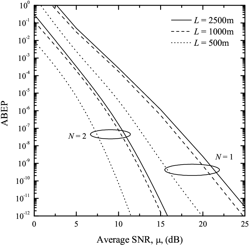
In Fig. 2, the dependence on the link distance of the ABEP of a MIMO OSM system is illustrated. The considered system is again equipped with either or receiving apertures and identically distributed branches are assumed. The parameters of the H-K distribution are calculated from (15) and (16) assuming spherical wave propagation. Following [39], it is further assumed that the operating wavelength is nm and . As expected, the error performance deteriorates as increases from m to m. Moreover, it is evident that an increase in from 500m to 1000m results in a more severe performance deterioration than in the case where increases from 1000m to 1500m. In all cases considered, the analytical results obtained using (26) are compared with the equivalent results obtained by means of Monte-Carlo computer simulations and again match very well.
Next we compare the proposed OSM system with two alternative coherent FSO systems that can provide performance enhancements by means of transmit (MISO) or receive diversity (SIMO). It is noted that for similar aperture configurations, a fair comparison between coherent and IM/DD systems seems difficult as the same received laser power leads to different SNRs for each of these schemes [23]. On the other hand, in order to perform a fair comparison between OSM and the alternative MISO or SIMO systems under the same propagation channel conditions, the aperture configuration of the FSO systems under comparison should be selected carefully. Specifically, because of the fact that the diversity gain of OSM equals to only the number of the receive apertures only, i.e. no transmit diversity gain is provided, the number of transmit or receive apertures of the alternative systems must be hence selected to be equal to the number of receive apertures of the OSM system. To this end, for a fair comparison in our paper a OSM system is compared with the following two alternative FSO communication systems which also employ coherent detection: i) A heterodyne FSO communication system which employs Differential Phase Shift Keying [25] and MRC or SC.
ii) A coherent FSO system employing the Alamouti scheme [22] and Binary Phase Shift Keying (BPSK).
The instantaneous SNR at the output of the coherent MRC receiver assuming equal average SNR per receiving aperture, can be expressed as [29]
| (46) |
whereas for SC is
| (47) |
For MRC case, the ABEP can be deduced as [29]
| (48) |
For SC case, an analytical expression for the ABEP is more difficult to be deduced and, therefore, ABEP will be evaluated by means of Monte Carlo simulation only.
As far as the Alamouti scheme is concerned, the instantaneous SNR at the input of the demodulator of the optical receiver has a similar form as (46) [22]. For this scheme, the ABEP of BPSK can be evaluated as
| (49) |
In order to simplify the underlying mathematical analysis, it is assumed that the PDF of is given by (9) with the parameters being all zero, i.e. the PDF is the K-distribution. Thus, can be readily obtained in closed form from (33) by replacing with . In Fig. 3, the ABEP of MIMO OSM links is compared with the ABEP of coherent FSO systems with DPSK. and identically distributed links are considered. In order to compare these systems under the same propagation conditions, it is assumed that , , and . As it can be observed, when either MRC or SC are employed, although coherent DPSK performs worse than OSM for values of up to approximately 1, it outperforms OSM at lower values of . Moreover, although the OSM outperforms the Alamouti scheme for and 3, it performs similarly for high SNR values when . It is noted that for and lower values of the Alamouti scheme yields the best performance of the considered OSM schemes. When more transmit appertures are employed, however, this advantage is compensated by the superior spectral efficiency of OSM and its lower hardware complexity as compared to coherent MRC. Specifically, as pointed out in [14], OSM offers increased spectral efficiency by a factor . Moreover, as only one transmitting aperture is activated at any symbol duration, OSM has a lower decoding complexity as compared to conventional MRC and Alamouti schemes.
In Fig. 4, upper bounds on the ABEP of convolutional coded and OSM systems are depicted, assuming similar propagation conditions to those considered in Fig. 2. Considering a convolutional code with rate and constraint length of 3, its transfer function is given as [40, Eq. (8.2.6)]
| (50) |
Substituting (50) to (43), a union bound on the ABEP can be obtained as
| (51) |
The performance results of Fig. 4 clearly show that, as expected, the incorporation of convolutional coding significantly enhances the performance of OSM systems, even when a small number of receive apertures is employed, even for .
VI Conclusion
In this paper, the use of spatial modulation technique for coherent FSO communication systems has been proposed. We have provided a comprehensive analytical framework for error performance analysis in the presence of atmospheric turbulence scattering channel models which include the H-K distribution. The proposed framework reveals important information about the performance of OSM over such turbulent channels, including the effect of fading severity and the achievable diversity gain. It also provides valuable insight into the impact of channel parameters on performance of OSM. Upper bounds for the ABEP performance of coded OSM systems have also been derived, demonstrating that coding techniques can greatly enhance the performance of OSM. Extensive computer simulation performance evaluation results have been also obtained which have verified the accuracy of the analytical approach. Important trends about the performance of OSM for a variety of atmospheric turbulent scenarios and MIMO setups have also been identified. For example, it was shown that OSM can provide significant performance enhancements in the presence of atmospheric turbulence. The improvements are comparable to the ones offered by conventional coherent systems with spatial diversity, while outperforming the latter in terms of spectral efficiency and hardware complexity. Besides, under specific propagation conditions, OSM can yield better performance than conventional SIMO systems employing MRC or SC. We believe that the proposed framework is a useful tool for understanding the performance trend, important properties and tradeoffs of outdoor OSM operating in the presence of atmospheric turbulence.
References
- [1] I. Gradshteyn and I. M. Ryzhik, Tables of Integrals, Series, and Products, 6th ed. New York: Academic Press, 2000.
- [2] X. Zhu and J. M. Kahn, “Free-space optical communications through atmospheric turbulence channels,” IEEE Transaction on Communications, vol. 50, no. 8, pp. 1293–1300, 2002.
- [3] A. Garcia-Zambrana, “Error rate performance for STBC in free-space optical communications through strong atmospheric turbulence,” IEEE Commun. Lett., vol. 11, no. 5, pp. 390–392, May 2007.
- [4] S. M. Navidpour, M. Uysal, and M. Kavehrad, “Performance of free-space optical transmission with spatial diversity,” IEEE Trans. Wireless Commun., vol. 6, no. 8, pp. 2813–2819, Aug. 2007.
- [5] K. Peppas, “A simple, accurate approximation to the sum of gamma-gamma variates and applications in MIMO free-space optical systems,” IEEE Photon. Technol. Lett., vol. 23, no. 13, pp. 839–841, Jul 2011.
- [6] K. Peppas, F. Lazarakis, A. Alexandridis, and K. Dangakis, “Simple, accurate formula for the average bit error probability of multiple-input multiple-output free-space optical links over negative exponential turbulence channels,” Optics Letters, vol. 37, pp. 3243–3245, Aug. 2012.
- [7] L. C. Andrews, M. A. Al-Habash, C. Y. Hopen, and R. L. Phillips, “Theory of optical scintillation: Gaussian beam wave model,” Waves in Random Media, vol. 11, pp. 271–291, 2001.
- [8] M. A. Al-Habash, L. C. Andrews, and R. L. Phillips, “Mathematical model for the irradiance PDF of a laser beam propagating through turbulent media,” Opt. Eng, vol. 40, no. 8, pp. 1554–1562, 2001.
- [9] J. H. Churnside and S. F. Clifford, “Log-normal Rician probability density function of optical scintillations in the turbulent atmosphere,” Journal of Optical Society of America, vol. 4, pp. 1923–1930, 1987.
- [10] E. Jakeman, “On the statistics of k-distributed noise,” J. Phys. A, vol. 13, pp. 31–48, 1980.
- [11] L. C. Andrews and R. L. Philips, “Mathematical genesis of the I-K distribution for random optical fields,” Journal of the Optical Society of America A, vol. 3, no. 11, pp. 1912–1919, 1986.
- [12] L. C. Andrews, R. L. Phillips, and K. Shivamoggi, “Relations of the parameters of the I-K distribution for irradiance fluctuations to physical parameters of the turbulence,” Applied Optics, vol. 27, no. 11, pp. 2150–2155, 1988.
- [13] K. P. Peppas, A. N. Stassinakis, G. K. Topalis, H. E. Nistazakis, and G. S. Tombras, “Average capacity of optical wireless communication systems over I-K atmospheric turbulence channels,” J. Opt. Commun. Netw., vol. 4, pp. 1026–1032, 2012.
- [14] R. Mesleh, H. Elgala, and H. Haas, “Optical spatial modulation,” J. Opt. Commun. Netw., vol. 3, no. 3, pp. 234–244, Mar. 2011.
- [15] R. Mesleh, H. Elgala, R. Mehmood, and H. Haas, “Performance of optical spatial modulation with transmitters-receivers alignment,” IEEE Commun. Lett., vol. 15, no. 1, pp. 79–81, Jan. 2011.
- [16] T. Fath and H. Haas, “Performance comparison of MIMO techniques for optical wireless communications in indoor environments,” IEEE Trans. Commun., vol. 61, no. 2, pp. 733–742, Feb. 2013.
- [17] Y. A. Chau and S.-H. Yu, “Space modulation on wireless fading channels,” in Proc. IEEE Veh. Technol. Conf. – Fall, vol. 3, 2001, pp. 1668–1671.
- [18] R. Y. Mesleh, H. Haas, S. Sinanovic, C. Ahn, and S. Yun, “Spatial modulation,” IEEE Trans. Veh. Technol., vol. 57, pp. 2228–2241, Jul. 2008.
- [19] R. Mesleh, M. D. Renzo, H. Haas, and P. M. Grant, “Trellis coded spatial modulation,” IEEE Trans. Wireless Commun., vol. 9, no. 7, pp. 2349–2361, Jul. 2010.
- [20] S.-H. Hwang and Y. Cheng, “SIM/SM-aided free-space optical communication with receiver diversity,” Journal of Lightwave Technology, vol. 32, no. 14, pp. 2443–2450, Jul. 2014.
- [21] T. Ozbilgin and M. Koca, “Optical spatial modulation over atmospheric turbulence channels,” Journal of Lightwave Technology, 2015, early Access Article, DOI 10.1109/JLT.2015.2409302.
- [22] M. Niu, J. Cheng, and J. F. Holzman, “Alamouti-type STBC for atmospheric optical communication using coherent detection,” IEEE Photonics Journal, 2014. [Online]. Available: http://ieeexplore.ieee.org/xpls/icp.jsp?arnumber=6725602
- [23] E. Bayaki and R. Schober, “Performance and design of coherent and differential space-time coded FSO systems,” Journal of Lightwave Technology, vol. 30, no. 11, pp. 1569–1577, Jun. 2012.
- [24] S. M. Aghajanzadeh and M. Uysal, “Diversity-multiplexing trade-off in coherent free-space optical systems with multiple receivers,” IEEE/OSA J. Opt. Commun. Netw., vol. 2, pp. 1087–1094, Dec. 2010.
- [25] K. Kiasaleh, “Performance of coherent DPSK free-space optical communication systems in k-distributed turbulence,” IEEE Trans. Commun., vol. 54, no. 4, pp. 604–607, Apr. 2006.
- [26] M. D. Renzo and H. Haas, “Space Shift Keying (SSK–) MIMO over correlated Rician fading channels: Performance analysis and a new method for transmit-diversity,” IEEE Trans. Commun., vol. 59, no. 1, pp. 116–129, Jan. 2011.
- [27] J. Jeganathan, A. Ghrayeb, and L. Szczecinski, “Spatial modulation: optimal detection and performance analysis,” IEEE Commun. Lett., vol. 12, no. 8, pp. 545–547, 2008.
- [28] J. W. Goodman, Statistical Optics. John Wiley and Sons, 1985.
- [29] M. K. Simon and M. S. Alouini, Digital Communication over Fading Channels, 2nd ed. New York: Wiley, 2005.
- [30] E. Lee and V. Chan, “Part 1: optical communication over the clear turbulent atmospheric channel using diversity,” IEEE J. Sel. Areas Commun., vol. 22, pp. 1896–1906, Nov. 2004.
- [31] N. Letzepis, I. Holland, and W. Cowley, “The Gaussian free space optical MIMO channel with Q–ary pulse position modulation,” IEEE Trans. Wireless Commun., vol. 7, pp. 1744–1753, May 2008.
- [32] M. Chiani, D. Dardari, and M. K. Simon, “New exponential bounds and approximations for the computation of error probability in fading channels,” IEEE Trans. Wireless Commun., vol. 2, pp. 840–845, Jul. 2003.
- [33] A. P. Prudnikov, Y. A. Brychkov, and O. I. Marichev, Integrals and Series Volume 4: Direct Laplace Transforms, 1st ed. CRC, 1992.
- [34] M. Abramovitz and I. Stegun, Handbook of Mathematical Functions with Formulas, Graphs, and Mathematical Tables. New York, ISBN 0-486-61272-4: Dover, 1964.
- [35] F. Yilmaz and M.-S. Alouini, “An MGF-based capacity analysis of equal gain combining over fading channels,” in Proc. IEEE PIMRC, Sep. 2010, pp. 945–950.
- [36] P. Theofilakos, A. G. Kanatas, and G. P. Efthymoglou, “Performance of generalized selection combining receivers in fading channels,” IEEE Commun. Lett., vol. 12, no. 11, pp. 816–818, Nov. 2008.
- [37] Z. Wang and G. Giannakis, “A simple and general parametrization quantifying performance in fading channels,” IEEE Trans. Commun., vol. 51, no. 8, pp. 1389–1398, Aug. 2003.
- [38] M. D. Renzo and H. Haas, “Bit error probability of space modulation over Nakagami- fading: Asymptotic analysis,” IEEE Commun. Lett., vol. 15, no. 10, pp. 1026–1028, Oct. 2011.
- [39] M. Uysal, J. T. Li, and M. Yu, “Error rate performance analysis of coded free-space optical links over gamma-gamma atmospheric turbulence channels,” IEEE Trans. Wireless Commun., vol. 5, no. 6, pp. 1229–1233, Jun. 2006.
- [40] J. G. Proakis, Digital Communications, 3rd ed. New York: Mc Graw Hill, 1995.