Minimum Cost Constrained Input-Output and Control Configuration Co-Design Problem: A Structural Systems Approach

Recently, the I/O selection problem have received increasing attention in the literature, especially, since the publication of [4]. In [4], the minimal controllability problem (MCP), i.e., the problem of determining the sparsest input matrix that ensures controllability of a given the system dynamics matrix, was shown to be NP-hard, and some greedy algorithms provided. Exact solutions to MCP are explored in [5], and in [6], using graph theoretical constructions, the minimal controllability problem is shown to be polynomially solvable for almost all numerical realizations of the dynamic matrix, satisfying a predefined pattern of zeros/nonzeros. Alternatively, in [7, 8, 9, 10] the configuration of actuators is sought to ensure certain performance criteria; more precisely, [7, 8, 10] focus on optimizing properties of the controllability Grammian, whereas [9] studies leader selection problems, in which leaders are viewed as inputs to the system, and the selection criteria aims to speed up convergence. In addition, in [9, 7, 8] the submodularity properties of functions of the controllability Grammian are explored, and design algorithms are proposed that achieve feasible placement with certain guarantees on the optimality gap. The I/O selection problem considered in the present paper differs from the aforementioned problems in the following two aspects: first, the selection of the inputs is restricted to belong to a specific given set of possible inputs, i.e., we study constrained input placement, and, hence, differing from [4, 5, 6] in which unconstrained input placement is studied. Secondly, it contrasts with [7, 8, 9, 10] in the sense that we do not aim to ensure performance in terms of a function of the controllability Grammian, but we aim to minimize the overall actuation cost, measured in terms of manufacturing/installation/preference costs. Furthermore, instead of optimizing a specific (numerical) system instance, we focus on structural design guarantees that hold for almost all (numerical) system instantiations with a specified dynamic coupling structure. In addition, within the scope of the present problem, we provide optimal solutions under mild assumptions on the dynamics of the system, under very general cost formulations. Note that, if we consider general dynamical systems, even with uniform cost, the problem tackled by us is NP-hard [11]. The latter problem is referred to as the minimal constrained input selection (CMIS) problem, i.e., the problem of determining the minimum number of inputs that ensures structural controllability, which has been extensively studied, see [12, 13] and references therein. In a sense, this provides justification for the traditional approaches to solve the I/O selection problem, which include suboptimal methods such as heuristics, genetic algorithms or relaxations, see for instance [14, 15, 16, 17, 18], and references therein.

Regarding the CC problem [14], it is worthy to point out that some meaningful advances were recently achieved in terms of determining the numerical gains to achieve closed-loop systems performance, given the existence of feasible informations patterns, that were accomplished by using convex optimization tools [19]. More precisely, the set of feasible solutions is often characterized in terms of a property called quadratic invariance, which has been subsequently shown to be necessary and sufficient [20], see also [21] for a review about the recent developments. Nevertheless, these methods always assume that there exists a feasible information pattern, and no restriction is imposed in terms of the sparsity or the cost incurred by a feasible information pattern. This is one of the goals of the present paper; in a sense, we can use the approach in the present paper to determine feasible information patterns that can, subsequently, be used to determine gains for numerical system instances using the existing tools. In [22] the design of wireless control networks is pursued, where given a decentralized plant, modeled as a discrete linear time invariant system equipped with actuators and sensors, the communication topology design between actuators and sensors to achieve decentralized control was posed as a CC selection problem. Both theoretical and computational perspectives were provided, although the CC selection problem admits a degree of simplification in the discrete time setting. The CC selection problem has also been considered in [23] where a method for determining the minimum number of essential inputs and outputs required for decentralization was provided; however, the characterization does not cope with all cases, see, for instance [24] (page 219). Another work that is related with ours is [25], which studies only the CC selection problem, for a given placement of inputs and outputs, i.e., the inputs and outputs do not incur in any cost. Furthermore, the methodology in [25] is not applicable when some of the communication costs are taken to be infinite, i.e., when a sensor cannot directly communicate with an actuator, as is often the case in many large-scale (possibly geographically distributed) systems.

Nevertheless, as also referred in [14] there are very few methods that address the I/O and CC problems jointly, and to the best of our knowledge none that considers general actuation/sensing and communication costs. Hereafter, we show that the problem is difficult (NP-hard) to solve in general, however, we identify an important subclass that admits polynomial complexity solutions. More precisely, we show that there exist efficient tools to address the I/O and CC selection co-design when the dynamics matrix is irreducible. Notice that this comprises a variety of inter-connected dynamical systems [26], multi-agent networks [26, 27], or dynamics based in consensus-like protocols [28, 27], where the irreducibility is essentially ensured by the network connectivity.

The closest work to the one presented in here, in the sense that it explores the I/O and control configuration co-design problem, is the one in [6], where the sparsest I/O selection and control configuration problems, under the assumption that only the structure of the system dynamics is known but without constraints on the possible inputs/outputs, were addressed. An extension of [6] was presented in [29], where general (possibly heterogeneous) costs to actuate and measure state variables, but with uniform communication or feedback link cost, was considered. However, the I/O cost structure considered in [29] is somewhat different from that considered in this paper; in the former, the cost is imposed on the state variables that are to be actuated/observed and not on the specific actuators/sensors as considered in $\mathcal{P}_{1}$ in this paper. In summary, the present work differs from that presented in [6, 29] in the following three major aspects: (i) it considers additional constraints on the possible inputs and outputs used; (ii) the costs depend on the inputs and outputs used to perform a task; and (iii) the communication cost between input-output pairs is arbitrary. $\circ$

The main contributions of this paper are as follows: (i) we show that the minimum cost constrained I/O and control configuration co-design problem is NP-hard; (ii) we present an efficient algorithm¹¹ 1 The Matlab implementation of the algorithm can be found in https://www.mathworks.com/matlabcentral/fileexchange/49977 (polynomial in the dimension of the state, input and output) to solve it, when the dynamic matrix is irreducible; and (iii) we show how our solution, when the dynamic matrix is irreducible, can be used to solve the minimum cost constrained I/O selection problem, and the minimum cost CC selection problem, individually.

The rest of the paper is organized as follows. In Section II, we provide the formal problem statement, together with some motivation. Section III reviews some concepts and introduces results in structural systems theory. Subsequently, in Section IV we present the main technical results (proofs are relegated to the Appendix), followed by an illustrative example in Section V. Conclusions and discussions on further research are presented in Section VI.

Let $c_{u}(i)\in\mathbb{R}^{n}_{+}$ denote the (non-negative) cost associated with selecting the $i$th input $u_{i}$ ($i\in\mathcal{I}=\{1,\ldots,p\}$), $c_{y}(j)\in\mathbb{R}^{n}_{+}$ denote the (non-negative cost) associated with selecting the $j$th output $y_{j}$ ($j\in\mathcal{J}=\{1,\ldots,m\}$), and $c_{f}((i,j))\in\mathbb{R}^{n}_{+}\cup\{\infty\}$, with $(i,j)\in\mathcal{I}\times\mathcal{J}$, denote the cost associated with feeding output $j$ to input $i$, also referred to as communication cost, where $c_{f}((i^{\prime},j^{\prime}))=\infty$ if output $j^{\prime}$ is not available to input $i^{\prime}$. This paper aims to study the following problem.

Due to the combinatorial nature of the I/O and CC co-design problems (see for instance [14]) are typically solved using a two-step (generally suboptimal) procedure, namely solving first the input/output (I/O) selection problem, followed by the control configuration (CC) selection problem. Formally, the structural theory counterparts of these problems are given as follows:

$\diamond$

A (computational) problem is said to be reducible in polynomial time to another if there exists a procedure to transform the former to the latter using a number of operations which is polynomial in the size of its inputs. Such a reduction is useful in determining the complexity class [33] a problem belongs to. For instance, recall that a problem $\mathcal{P}$ in NP (i.e., the class of non-deterministic polynomial algorithms) is said to be NP-complete if all other NP problems can be polynomially reduced to $\mathcal{P}$ [33]. The set of NP-complete problems is referred to as the NP-complete class. The following result may be used to prove the NP-completeness of a given problem.

The NP-complete class is used to describe the complexity of decision versions of problems. For instance, the following constitutes a decision problem that is particularly relevant in the structural design context: Given $\bar{A}\in\{0,1\}^{n\times n}$ and $\bar{B}\in\{0,1\}^{n\times p}$, is there a collection of inputs $\bar{B}(\mathcal{J})$, where $\mathcal{J}\subset\{1,\ldots,p\}$ and where $\bar{B}(\mathcal{J})$ corresponds to the sub-matrix of $\bar{B}$ comprising the columns with indices in $\mathcal{J}$, with $|\mathcal{J}|=k$ such that $(\bar{A},\bar{B}(\mathcal{J}))$ is structurally controllable?

Alternatively, it is often natural to consider the optimization versions associated with the decision problems. For instance, the optimization version of the problem stated above aims to determine the minimum $k$ such that the aforementioned property holds. This optimization problem is referred to as the constrained minimum structural input selection (CMIS) problem, given by $\mathcal{P}_{1}^{\text{I/O}}$ with uniform non-zero actuation costs. Note that, if a solution to the optimization problem is known, the decision problem is straightforward to solve. Consequently, the optimization problem formulations of NP-complete problems, are referred to as being NP-hard, since they are at least as difficult as the NP-complete problems; in other words, by solving an instance of the optimization problem (the NP-hard problem), one can obtain a solution to an NP-complete problem.

The following standard terminology and notions from graph theory can be found, for instance, in [6]. Let $\mathcal{D}(\bar{A})=(\mathcal{X},\mathcal{E}_{\mathcal{X},\mathcal{X}})$ be the digraph representation of $\bar{A}$ in (1), where the vertex set $\mathcal{X}$ represents the set of state variables (also referred to as state vertices) and $\mathcal{E}_{\mathcal{X},\mathcal{X}}=\{(x_{i},x_{j}):\ A_{ji}\neq 0\}$ denotes the set of edges. Similarly, we define the following digraphs: $\mathcal{D}(\bar{A},\bar{B})=(\mathcal{X}\cup\mathcal{U},\mathcal{E}_{\mathcal{X},\mathcal{X}}\cup\mathcal{E}_{\mathcal{U},\mathcal{X}})$ where $\mathcal{U}$ represents the set of input vertices and $\mathcal{E}_{\mathcal{U},\mathcal{X}}=\{(u_{i},x_{j}):\ \bar{B}_{ji}\neq 0\}$; and $\mathcal{D}(\bar{A},\bar{B},\bar{K},\bar{C})=(\mathcal{X}\cup\mathcal{U}\cup\mathcal{Y},\mathcal{E}_{\mathcal{X},\mathcal{X}}\cup\mathcal{E}_{\mathcal{X},\mathcal{Y}}\cup\mathcal{E}_{\mathcal{U},\mathcal{X}}\cup\mathcal{E}_{\mathcal{Y},\mathcal{U}})$ denotes the digraph associated with the closed-loop system, where $\mathcal{Y}$ represents the set of output vertices and $\mathcal{E}_{\mathcal{X},\mathcal{Y}}=\{(x_{i},y_{j}):\ \bar{C}_{ji}\neq 0\}$ and the set of feedback edges/links is given by $\mathcal{E}_{\mathcal{Y},\mathcal{U}}=\{(y_{i},u_{j}):\ \bar{K}_{ji}\neq 0\}$.

A digraph $\mathcal{D}_{s}=(\mathcal{V}_{s},\mathcal{E}_{s})$ with $\mathcal{V}_{s}\subset\mathcal{V}$ and $\mathcal{E}_{s}\subset\mathcal{E}$ is called a subgraph of $\mathcal{D}$. If $\mathcal{V}_{s}=\mathcal{V}$, $\mathcal{D}_{s}$ is said to span $\mathcal{D}$. Finally, a subgraph with some property $P$ is maximal if there is no other subgraph $\mathcal{D}_{s^{\prime}}=(\mathcal{V}_{s^{\prime}},\mathcal{E}_{s^{\prime}})$ of $\mathcal{D}$, such that $\mathcal{D}_{s}$ is a subgraph of $\mathcal{D}_{s^{\prime}}$, and $\mathcal{D}_{s^{\prime}}$ satisfies property $P$. A sequence of directed edges $\{(v_{1},v_{2}),(v_{2},v_{3}),\cdots,(v_{k-1},v_{k})\}$, in which all the vertices are distinct, is called an elementary path from $v_{1}$ to $v_{k}$, as well as a vertex in a digraph with no incoming and outgoing edges (with some abuse of terminology). A vertex with an edge to itself (i.e., a self-loop), or an elementary path from $v_{1}$ to $v_{k}$ comprising an additional edge $(v_{k},v_{1})$, is called a cycle.

In addition, a digraph $\mathcal{D}$ is said to be strongly connected if there exists an elementary path between any pair of vertices. A strongly connected component (SCC) is a maximal subgraph $\mathcal{D}_{S}=(\mathcal{V}_{S},\mathcal{E}_{S})$ of $\mathcal{D}$ such that for every $v,w\in\mathcal{V}_{S}$ there exists a path from $v$ to $w$ and from $w$ to $v$.

Using the above constructions, we can now present some graph theoretical properties that the digraph associated with the closed-loop system $\mathcal{D}(\bar{A},\bar{B},\bar{C},\bar{K})$ must satisfy to avoid the existence of SFMs.

The conditions in Theorem 1 hold only if the system is both structurally controllable and structurally observable²² 2 A system $(\bar{A},\bar{C})$ is said to be structurally observable if there exists an observable pair $(A_{0},C_{0})$ with zero entries enforced by the zero entries in $(\bar{A},\bar{C})$.. More precisely, we have the following result.

The optimal assignment problem consists in determining the collection $\mathcal{M}^{*}$ of pairs of indices of a $k\times k$ square matrix $H$ that correspond to the diagonal entries of the matrix $P_{1}^{*}HP_{2}^{*}$, where $P_{1}^{*}$ and $P_{2}^{*}$ are permutation matrices such that

with $\mathcal{P}$ denoting the class of all $k\times k$ permutation matrices. In what follows, we consider, for the optimal assignment problem, block matrices $H$ given by

where the labels of the columns associated with the first block are $\{x_{1},\ldots,x_{n}\}$, the second $\{u_{1},\ldots,u_{p}\}$, and the third $\{y_{1},\ldots,y_{m}\}$. Similarly, the labels of the rows associated with the first block are $\{x_{1},\ldots,x_{n}\}$, the second $\{u_{1},\ldots,u_{p}\}$, and the third $\{y_{1},\ldots,y_{m}\}$. For example, the first row and third column of the $n\times n$ matrix $H^{xx}_{n\times n}$ is indexed by the pair $(x_{1},x_{3})$, and the first row and third column of the $n\times p$ matrix $H^{u,x}_{n\times p}$ is indexed by the pair $(u_{1},x_{3})$. Consequently, any solution to the optimal assignment problem $\mathcal{M}^{*}\subset\mathcal{L}\times\mathcal{L}$, where $\mathcal{L}=\{x_{1},\ldots,x_{n},u_{1},\ldots,u_{p},y_{1},\ldots,y_{m}\}$, consists of $n+p+m$ pairs of indices.

Further, we can associate a matrix $H$ with a digraph representation $\mathcal{D}(H)=(\mathcal{L},\mathcal{E})$, where $\mathcal{E}\subseteq\mathcal{L}\times\mathcal{L}$. In particular, a matrix $H$ is irreducible if and only if $\mathcal{D}(H)$ is an SCC. In addition, we have the following result given by König (see Appendix in [35]):

Let the structure of the dynamics, input and output matrices be given as follows:

In addition, let the input costs are given by $c_{u}=[10\ 10\ 20\ 20]$, the output costs by $c_{y}=[15\ 15\ 50]$, and the communication costs by

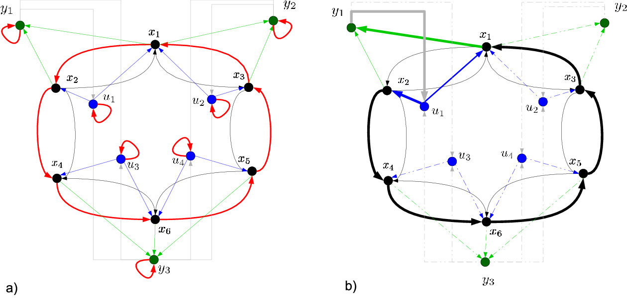
First, notice that $\bar{A}$ is irreducible, and we can resort to Algorithm 1 to solve $\mathcal{P}_{1}$. After we execute Algorithm 1, the solution obtained is $\mathcal{I}^{*}=\{1\}$, $\mathcal{J}^{*}=\{1\}$ and $\mathcal{F}^{*}=\{(1,1)\}$, illustrated in Figure 1-b) by the non-black and non-dashed edges, and incurring in a total cost of $30$.

Let the structure of the dynamics, input and output matrices be given as follows:

In addition, let the input costs are given by $c_{u}=[5\ 10\ 10]$, the output costs by $c_{y}=[10\ 10\ 1]$, and the communication costs by

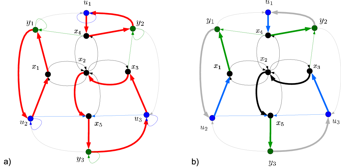
First, notice that $\bar{A}$ is irreducible, and we can resort to Algorithm 1 to solve $\mathcal{P}_{1}$. The solution obtained is $\mathcal{I}^{*}=\{1,2,3\}$, $\mathcal{J}^{*}=\{1,2,3\}$ and $\mathcal{F}^{*}=\{(2,1),(3,3),(1,2)\}$, illustrated in Figure 2-b) by the non-black and non-dashed edges, and incurring in a total cost of $186$.

To prove that $\mathcal{P}_{1}$ is NP-hard, we provide a reduction from a known NP-hard problem, the CMIS (see Section II, problem $\mathcal{P}_{1}^{\text{I/O}}$), to a particular instance of $\mathcal{P}_{1}$ when the costs (input/output/communication) are equal and uniform, which we refer to as $\mathcal{P}_{1}^{\prime}$. Consequently, the corresponding decision problems can be polynomially reduced to each other, and the result follows by invoking Lemma 1. First, we notice that it is possible to polynomially verify if a solution to $\mathcal{P}_{1}^{\prime}$ is feasible, and, consequently, to the corresponding decision problem, see, for instance [25]; hence, the decision version of $\mathcal{P}_{1}^{\prime}$ is an NP problem. Now, we construct a polynomial reduction from the CMIS problem to $\mathcal{P}_{1}^{\prime}$. Towards this goal, let $\bar{A}$, $\bar{B}$ and $c_{u}(i)$, $i\in\mathcal{I}=\{1,\ldots,p\}$, in $\mathcal{P}_{1}^{\prime}$ be the same as in the CMIS problem. In addition, let $\bar{C}=\mathbb{I}_{n}$ be the $n\times n$ identity matrix, $c_{y}(j)=0$ for $j\in\mathcal{J}=\{1,\ldots,n\}$ and $c_{f}((i,j))=0$ for $(i,j)\in\mathcal{I}\times\mathcal{J}$. To see that a solution to the proposed problem $\mathcal{P}_{1}^{\prime}$ provides us with a solution to CMIS, recall that a feasible solution to $\mathcal{P}_{1}^{\prime}$, i.e., $(\bar{A},\bar{B},\bar{C},\bar{K})$ without SFMs, implies that $(\bar{A},\bar{B})$ is structurally controllable (see Proposition 1). Now, to see that $B(\mathcal{I}^{*})$ in $\mathcal{P}_{1}^{\prime}$ is also a solution to CMIS, let us assume, by contradiction that it is not. Then, there exists $\mathcal{I}^{\prime}$ such that $\bar{B}(\mathcal{I}^{\prime})$ incurs in a lower cost than $\bar{B}(\mathcal{I})$, and such that $(\bar{A},\bar{B}(\mathcal{I}^{\prime}))$ is structurally controllable. Now, because $\bar{C}$ is the identity matrix and $\bar{K}$ can be full without increasing the cost, it follows that there exists a collection of cycles that comprise the inputs labeled by $\mathcal{I}^{\prime}$, as well as a set of labels for the outputs and feedback given by $\mathcal{J}^{\prime}$ and $\mathcal{F}^{\prime}$, respectively. However, this collection of cycles provides with a solution $\mathcal{M}^{\prime}$ to the optimal assignment problem that incurs in lower cost than $\mathcal{M}^{*}$, which is a contradiction since we assumed that $\mathcal{M}^{*}$ is a solution to the optimal assignment problem. $\blacksquare$

As discussed in the preliminaries, a solution $\mathcal{M}^{*}$ to the optimal assignment problem of $\mathcal{C}^{*}$ always provides a collection of $n+m+p$ pairs of labels of the form $\mathcal{M}^{*}\subset\mathcal{L}\times\mathcal{L}$, where $\mathcal{L}=\{x_{1},\ldots,x_{n},u_{1},\ldots,u_{p},y_{1},\ldots,y_{m}\}$. Subsequently, by construction of $\mathcal{C}^{*}$, if the weight-sum cost of the entries in $\mathcal{C}^{*}$ labeled in $\mathcal{M}^{*}$ is finite, then there exists a collection of disjoint cycles in the digraph representation of $\mathcal{C}^{*}$ (see Proposition 2). Now, notice that by construction, only edges associated to finite entries in $\mathcal{C}^{*}$ are used; hence, the cycles comprise only edges of the form $(x_{i},x_{j})$, $(u_{i},x_{j})$, $(x_{i},y_{j})$, $(y_{j},u_{i})$, as well as $(u_{i},u_{i})$ and $(y_{j},y_{j})$. Further, the latter edges $(u_{i},u_{i})$ and $(y_{j},y_{j})$ do not contribute to ensure either condition a) or b) in Theorem 1, nor are they represented in $\mathcal{D}(\bar{A},\bar{B},\bar{C},\bar{K})$; hence, they can be neglected from the analysis. Subsequently, by noticing that if any edge of the form $(u_{i},x_{j})$, $(x_{i},y_{j})$, $(y_{j},u_{i})$ belongs to $\mathcal{M}^{*}$, then so are the other two, otherwise, $\mathcal{M}^{*}$ does not comprise a family of cycles with finite weight. Nonetheless, it might be the case that there is no edge of the form $(u_{i},x_{j})$, $(x_{i},y_{j})$, $(y_{j},u_{i})$, that corresponds to the case where $\mathcal{M}^{\prime}$ incurs in finite cost, which implies that there exists a disjoint union of cycles comprising only vertices with labels $\{x_{1},\ldots,x_{n}\}$; subsequently, all edges of the form $(u_{j},u_{j})$ and $(y_{k},y_{k})$ are used in $\mathcal{M}^{*}$. In this case, the weight-sum of $\mathcal{M}^{*}$ is equal to zero and, although condition Theorem 1-b) is satisfied, it follows that there is no edge of the form $(y_{i},u_{j})$ in the SSC containing the state variables in $\mathcal{D}(\bar{A},\bar{B},\bar{C},\bar{K})$. To preclude this case, if $\mathcal{M}^{\prime}$ incurs in finite cost, we consider the triple $(\bar{B}(\{i\}),\bar{C}(\{j\}),\bar{K}(\{(i,j)\}))$ that incurs in the smallest cost; hence, condition Theorem 1-a) is satisfied, and Theorem 1 holds. Alternatively, if $M^{\prime}$ does not incur in finite cost, then additional edges that are not of the form $(x_{i},x_{j})$ are required to be associated with a solution to the optimal assignment problem, as result of Proposition 2. Further, both conditions in Theorem 1 are satisfied: more precisely, a) is satisfied since $\mathcal{D}(\bar{A})$ is an SCC (by assumption), and there must exist at least an edge of the form $(y_{j},u_{i})$ in $\mathcal{M}^{*}$, as well as in $\mathcal{D}(\bar{A},\bar{B}(\mathcal{I}^{*}),\bar{C}(\mathcal{J}^{*}),\bar{K}(\mathcal{F}^{*}))$ obtained using Algorithm 1. On the other hand, Theorem 1-b) is satisfied by considering, the edges of a solution to the optimal assignment problem used to define $\mathcal{D}(\bar{A},\bar{B}(\mathcal{I}^{*}),\bar{C}(\mathcal{J}^{*}),\bar{K}(\mathcal{F}^{*}))$.

Finally, we notice that the algorithm’s complexity is $\mathcal{O}((n+m+p)^{3})$, since it is the complexity of applying the Hungarian algorithm to the optimal assignment problem associated with $\mathcal{C}^{*}$; all the remaining steps have lower complexity which renders them moot to the final complexity. $\blacksquare$

First, we notice that since $\bar{A}$ is irreducible, from Theorem 3, it follows that Algorithm 1 determines the optimal solution to $\mathcal{P}_{1}$. Further, if $(\bar{A},\bar{B},\bar{C},\bar{K})$ has no SFMs, then it is structurally controllable and observable (see Proposition 1). Because we have that the system is structurally observable and all outputs can be fed to all inputs without increasing the cost, it follows that the problem consists in determining the collection of inputs that incurs in the minimum cost; hence, by noticing that this is the same as the $\mathcal{P}_{1}^{\text{I/O}}$, the result follows. $\blacksquare$

References

- [1] S. Skogestad, “Control structure design for complete chemical plants,” Computers and Chemical Engineering, vol. 28, no. 1-2, pp. 219–234, 2004.
- [2] S. Pequito, Q. Liu, S. Kar, and M. D. Ilic, “PMU placement to ensure observable frequency and voltage dynamics: A structured system approach,” in System Sciences (HICSS), 2013 46th Hawaii International Conference on, Jan 2013, pp. 2327–2336.
- [3] M. Mesbahi and M. Egerstedt, Graph theoretic methods in multiagent networks. Princeton University Press, 2010. [Online]. Available: http://www.worldcat.org/isbn/9780691140612
- [4] A. Olshevsky, “Minimal controllability problems,” Control of Network Systems, IEEE Transactions on, vol. 1, no. 3, pp. 249–258, Sept 2014.
- [5] S. Pequito, G. Ramos, S. Kar, A. P. Aguiar, and J. Ramos, “On the Exact Solution of the Minimal Controllability Problem,” ArXiv e-prints, Jan. 2014. [Online]. Available: http://arxiv.org/abs/1401.4209
- [6] S. Pequito, S. Kar, and A. P. Aguiar, “A framework for structural input/output and control configuration selection of large-scale systems,” Submitted to IEEE Transactions on Automatic Control, 2013. [Online]. Available: http://arxiv.org/abs/1309.5868
- [7] T. H. Summers, F. L. Cortesi, and J. Lygeros, “On Submodularity and Controllability in Complex Dynamical Networks,” ArXiv e-prints, Apr. 2014.
- [8] V. Tzoumas, M. A. Rahimian, G. J. Pappas, and A. Jadbabaie, “Minimal Actuator Placement with Bounds on Control Effort,” ArXiv e-prints, Sep. 2014.
- [9] A. Clark, B. Alomair, L. Bushnell, and R. Poovendran, “Minimizing convergence error in multi-agent systems via leader selection: A supermodular optimization approach,” Automatic Control, IEEE Transactions on, vol. 59, no. 6, pp. 1480–1494, June 2014.
- [10] F. Pasqualetti, S. Zampieri, and F. Bullo, “Controllability metrics, limitations and algorithms for complex networks,” Control of Network Systems, IEEE Transactions on, vol. 1, no. 1, pp. 40–52, March 2014.
- [11] S. Pequito, S. Kar, and A. P. Aguiar, “On the NP-completeness of the Constrained Minimal Structural Controllability/Observability Problem,” ArXiv e-prints, Mar. 2014.
- [12] C. Commault and J.-M. Dion, “Input addition and leader selection for the controllability of graph-based systems.” Automatica, vol. 49, no. 11, pp. 3322–3328, 2013.
- [13] J.-M. Dion, C. Commault, and J. V. der Woude, “Generic properties and control of linear structured systems: a survey.” Automatica, pp. 1125–1144, 2003.
- [14] M. van de Wal and B. de Jager, “A review of methods for input/output selection,” Automatica, vol. 37, no. 4, pp. 487 – 510, 2001.
- [15] S. L. Padula and R. K. Kincaid, “Optimization strategies for sensor and actuator placement,” National Aeronautics and Space Administration Langley Research Center, Langley, Virginia 23681, Tech. Rep., 1999.
- [16] M. Meyer, J. L. Lann, B. Koehret, and M. Enjalbert, “Optimal selection of sensor location on a complex plant, using a graph oriented approach,” Computers and Chemical Engineering, vol. 18, Supplement 1, no. 0, pp. S535 – S540, 1994.
- [17] M. I. Frecker, “Recent advances in optimization of smart structures and actuators,” Journal of Intelligent Material Systems and Structures, vol. 14, no. 4-5, pp. 207–216, 2003.
- [18] D. W. Begg and X. Liu, “On simultaneous optimization of smart structures - part II: Algorithms and examples,” Computer Methods in Applied Mechanics and Engineering, vol. 184, no. 1, pp. 25 – 37, 2000.
- [19] M. Rotkowitz and S. Lall, “A characterization of convex problems in decentralized control,” IEEE Transactions on Automatic Control, vol. 51, no. 2, pp. 274–286, Feb 2006.
- [20] L. Lessard and S. Lall, “Quadratic invariance is necessary and sufficient for convexity,” in American Control Conference (ACC), 2011, June 2011, pp. 5360–5362.
- [21] A. Mahajan, N. Martins, M. Rotkowitz, and S. Yuksel, “Information structures in optimal decentralized control,” in Decision and Control (CDC), 2012 IEEE 51st Annual Conference on, Dec 2012, pp. 1291–1306.
- [22] M. Pajic, R. Mangharam, G. Pappas, and S. Sundaram, “Topological conditions for in-network stabilization of dynamical systems,” Selected Areas in Communications, IEEE Journal on, vol. 31, no. 4, pp. 794–807, April 2013.
- [23] M. Sezer, “Minimal essential feedback patterns for pole assignment using dynamic compensation,” Proceedings of the 22th IEEE Conference on Decision and Control, 1983.
- [24] L. Trave, A. Titli, and A. Tarras, Large Scale Systems: Decentralization, Structure Constraints, and Fixed Modes, ser. Lecture Notes in Control and Information Sciences. Springer-Verlag, 1989.
- [25] K. Unyelioglu and M. E. Sezer, “Optimum feedback patterns in multivariable control systems,” International Journal of Control, vol. 49, no. 3, pp. 791–808, 1989.
- [26] G. Antonelli, “Interconnected dynamic systems: An overview on distributed control,” Control Systems, IEEE, vol. 33, no. 1, pp. 76–88, Feb 2013.
- [27] A. Jadbabaie, J. Lin, and A. Morse, “Coordination of groups of mobile autonomous agents using nearest neighbor rules,” IEEE Transactions on Automatic Control, vol. 48, no. 6, pp. 988–1001, june 2003.
- [28] A. G. Dimakis, S. Kar, J. M. F. Moura, M. G. Rabbat, and A. Scaglione, “Gossip algorithms for distributed signal processing.” Proceedings of the IEEE, vol. 98, no. 11, pp. 1847–1864, 2010.
- [29] S. Pequito, S. Kar, and A. Aguiar, “Minimum cost input-output and control configuration selection: A structural systems approach,” in Decision and Control (CDC), 2013 IEEE 52nd Annual Conference on, Dec 2013, pp. 4895–4900.
- [30] S.-H. Wang and E. Davison, “On the stabilization of decentralized control systems,” IEEE Transactions on Automatic Control, vol. 18, no. 5, pp. 473 – 478, oct 1973.
- [31] C. H. Papadimitriou and J. Tsitsiklis, “A simple criterion for structurally fixed modes,” Systems & Control Letters, vol. 4, no. 6, pp. 333 – 337, 1984. [Online]. Available: http://www.sciencedirect.com/science/article/pii/S0167691184800742
- [32] M. Sezer and D. Siljak, “Structurally fixed modes,” Systems & Control Letters, vol. 1, no. 1, pp. 60–64, Jul. 1981. [Online]. Available: http://dx.doi.org/10.1016/S0167-6911(81)80014-X
- [33] M. R. Garey and D. S. Johnson, Computers and Intractability: A Guide to the Theory of NP-Completeness. New York, NY, USA: W. H. Freeman & Co., 1979.
- [34] V. Pichai, M. E. Sezer, and D. D. Siljak, “Brief paper: A graph-theoretic characterization of structurally fixed modes,” Automatica, vol. 20, no. 2, pp. 247–250, Mar. 1984.
- [35] K. J. Reinschke, Multivariable control: a graph theoretic approach, ser. Lecture Notes in Control and Information Sciences. Springer-Verlag, 1988, vol. 108.