We explore vacuum degeneracy of Kronecker quiver with large ranks, by computing Witten index of corresponding 1d gauged linear sigma model. For $(d-1,d)_{k}$ quivers with the intersection number $k$ , we actually counted index of its mutation equivalent, $(d,(k-1)d+1)_{k}$ , and find exponentially large behaviour whenever $k\geq 3$ . We close with speculation on more general ranks of Kronecker quiver including the nonprimitive cases.

1 Introduction

Wall-crossing phenomena and, more generally, the counting of degeneracy of BPS states have played a central role during last twenty years of development in superstring theory and supersymmetric gauge theories. BPS states, which preserves part of supersymmetry of the underlying field theory or gravity, are supposed to be robust due to the short supermultiplet structure they come with. This often allows us to probe otherwise inaccessible non-perturbative aspects, such as U-dualty between different string theories or even the grand idea of M-theory. With smaller supersymmetry preserved, however, this is not always reliable, and a theory sometimes loses or gains BPS states suddenly under continuous deformation of parameters, hence the wall-crossing phenomena. [1, 2, 3, 4]

Arguably, the most versatile framework where the intrinsic degeneracy of BPS states can be counted is the quiver quantum mechanics. This can be motivated rather simply by considering collections of D-branes that are completely wrapped on supersymmetric cycles in Calabi-Yau 3-fold. For compact Calabi-Yau’s, such a collection corresponds to BPS black holes while for noncompact ones, to BPS states. This line of approach was initiated by Douglas et al., [5, 6] and extensively developed by Denef’s pioneering work [7] which inspired a lot of physics and mathematics study of the wall-crossing. [8, 9, 10, 11, 12]

Nevertheless, direct and systematic counting of BPS states starting with quiver quantum mechanics became available only very recently. Problem of counting wall-crossing discontinuity is often simpler than counting degeneracies themselves. The so-called Coulomb approximation, which is inspired by the multi-center picture of wall-crossing came to fruition in Refs.[13, 14, 15, 16, 17, 18, 19], which is however later seen to miss a lot of physical states, when the quiver in question involves oriented loops of bifundamental chiral multiplets. Honest and comprehensive counting of Witten index was finally formulated in Ref. [20, 21, 23] not only for quiver theories but also for general gauged linear sigma models (GLSM), whose main result is phrased in terms of residue formulae in the space of gauge field expectation values. Section 3 below will summarize the result.

Despite such developments, one aspects of the BPS state counting remains much obscure. Namely, how the degeneracy scales as a function of the increasing charge. This question itself is of course very familiar in the context of BPS black holes, with the obvious answer being ”exponentially large,” yet most of definite answers on such a question are found in systems where wall-crossing is either absent or rather simple. Black holes that preserve four supercharges only and are BPS states in the supergravity theory that preserves eight supercharges, microstate counting in general is still unavailable. Isolating the correct exponential behaviour from microstate counting based on wrapped D-branes would be most useful, but this looks rather difficult technically despite the above residue formula as the number of residue integral to do grows linearly with charge, and the number of poles to consider itself grows exponentially fast.

On the other hand, the exponential behaviour of the degeneracy turns out to be present also in certain field theory BPS states, albeit to a lesser degree. This was initially anticipated by Kol [24] on the basis of string-web picture of 1/4 BPS dyons in ${\cal N}=4$ field theory in four dimensions. While the former’s argument is somewhat anecdotal, a more definite counting using low energy dynamics of solitons has shown how a highly charges states in field theory can be equipped with an exponentially large degeneracy. This exponential behaviour is different from that was anticipated with black holes in the following sense. For BPS black holes in four dimensional ${\cal N}=2$ supergravity, the scaling is such that

\Omega_{BH}\sim e^{\#\Gamma^{2}}\ ,

for a large charge $\Gamma$ , while for field theory BPS states the anticipated scaling goes like

\Omega\sim e^{\#\sqrt{\Gamma^{2}}}\ .

For either, one must deal with quiver quantum mechanics of large rank $\sim\Gamma$ , and the direct computation become exponentially difficult even with the general formulation of Witten index computation, unless one finds a mitigating circumstance.

This note is an attempt to reproduce such an exponential behaviour in the simplest possible nontrivial quiver, namely the Kronecker quiver, in the hope of finding more general systematics of large rank quiver dynamics. After a cursory introduction to quiver quantum mechanics, we go on in section 3 to describe how the Witten index of the Kronecker quiver of rank $d$ and $d-1$ can be computed via diagrammatical representation of the residue formula, following the method in Ref. [20]. A useful middle step in this computation is a mutation which take $(d-1,d)$ Kronecker quiver to $(d,(k-1)d+1)$ Kronecker quiver where $k$ is the common intersection number. We briefly discuss how this duality for these quivers could be realized in this context. Especially we obtained

\Omega_{(d,(k-1)d+1)_{k}}=\frac{1}{d}~[x^{(k-1)d+1}]g_{k}(x)=\frac{k}{d((k-1)d+1)}{(k-1)^{2}d+(k-1)\choose d-1}\ ,

(1.1)

which implies the scaling bahaviour

\lim_{d\rightarrow\infty}\Omega_{(d-1,d)_{k}}=\lim_{d\rightarrow\infty}\Omega_{(d,(k-1)d+1)_{k}}\sim e^{f(k)d}\ ,

(1.2)

where $f(k)=(k-1)^{2}\ln(k-1)^{2}-(k^{2}-2k)\ln(k^{2}-2k)$ . The result is consistent with the Euler number of quiver moduli spaces which has been widely discussed in the mathematical literature [26, 27] and in the context of spectral network [28]. We close with some further speculations in section 5.

As this work was completed, a paper [29] with some overlap has appeared in the ArXiv.

2 The Kronecker Quiver and Mutation

The simplest setting where quiver quantum mechanics emerges is type IIB theory compactified on Calabi-Yau 3-fold. The effective theory in the remaining four dimensions carries ${\cal N}=2$ supersymmetry, and the BPS state thereof are realized as D3-branes wrapped on special Lagrange subcycles of the Calabi-Yau. When the cycle is rigid, as with $S^{3}$ , the vector multiplet on the D3-brane reduces to quantum mechanical vector multiplet whose content is the same as ${\cal N}=1$ vector multiplet in four dimensions. If D3 wraps the same cycle $d$ times, the gauge theory is elevated to $U(d)$ . For each such D3-branes on $S^{3}$ , we can associate a Fayet-Iliopoulos constant $\zeta$ such that the low energy effective action carries a term

-\zeta\int dt\;{\rm tr}\,D\ ,

(2.1)

where $D$ is auxiliary field in the vector multiplet. When a pair of such wrapped D3’s, say each wrapping $d_{1}$ and $d_{2}$ times, meets at $k$ intersections, one find additional chiral multiplets in the bifundamental representation $(\bar{d}_{2},d_{1})$ . Such a quiver, which is the simplest possible nontrivial class, is called Kronecker quiver. We have the supersymmetry constraint

d_{1}\zeta_{1}+d_{2}\zeta_{2}=0\ ,

(2.2)

so we really have only one FI constant, say, $\xi\equiv d_{1}\zeta_{1}=-d_{2}\zeta_{2}$ . For negative $\xi$ the classical vacuum moduli space is null and so is the Witten index. For positive $\xi$ , the moduli space is given as a Kaehler quotient,

\{\Phi^{1,2,\dots,k}\in{\mathbb{C}}^{d_{2}}\times{\mathbb{C}}^{d_{1}}\;|\;\Phi^{\dagger}\cdot\Phi=\zeta_{1}\}/S\left(U(d_{1})\times U(d_{2})\right)\ .

(2.3)

The number of stable BPS bound states can be obtained by calculating indices of these quiver quantum mechanics. Furthermore, the theory has $SU(2)_{L}\times U(1)_{R}$ R-symmetry, where $SU(2)_{L}$ came from the rotational symmetry of the three spatial direction. We can refine the indices by turning on the fugacity ${\bf y}$ for $J_{3}+I$ of R-symmetry. Due to the pioneering work of Reineke [30] and Manschot et al. [14, 15], the systematic procedure of evaluating the equivariant indices of mutually co-prime quiver $(d_{1},d_{2})$ are viable. However, since they are given in terms of very particular sum of partitions of charges, it is hard to examine the large $d$ behaviour with those formula.

Indices for $k=1,2$ Kronecker quivers are well-documented and also easy to compute directly. Note that the complex dimension of the classical Higgs moduli space when $\xi>0$ is

{\rm dim}{\cal M}_{(d_{1},d_{2})_{k}}=k\cdot d_{1}\cdot d_{2}-(d_{1}^{2}+d_{2}^{2}-1)=1+(k-2)\cdot d_{1}\cdot d_{2}-(d_{1}-d_{2})^{2}\ .

This counting is misleading for nonprimitive cases such as $(d,d)$ , since the noncompact classical moduli spaces open up along the Coulomb direction. Direct evaluation of the standard formula leads to fractional quantities, but with more care the true integral index can be computed. With $k=1$ , the only primitive case with nonnegative dimension, thus nonempty moduli space, is $d_{1}=d_{2}=1$ . This case generates the most basic wall-crossing pattern, corresponding to the so-called pentagon-identity, and the index is

\Omega_{(1,1)_{1}}=1\ .

(2.4)

With $k=2$ , there are two classes with nonempty moduli spaces. The first is $d_{1}=d_{2}=1$ with ${\rm dim}{\cal M}_{(1,1)_{2}}=1$ and the second is $|d_{1}-d_{2}|=1$ with ${\rm dim}{\cal M}_{(d,d\pm 1)_{2}}=0$ . Indices for these can be inferred to the well-known spectrum of $SU(2)$ Seiberg-Witten theory, and also have been computed directly by several different methods. The answers are of course,

\displaystyle\Omega_{(1,1)_{2}}=-\frac{1}{{\bf y}}-{\bf y}\ ,

(2.5)

and

\displaystyle\Omega_{(d,d-1)_{2}}=\Omega_{(d-1,d)_{2}}=1\ .

(2.6)

Seiberg-Witten wall-crossing formula implies that there are no other nontrivial indices in this class, meaning also that all nonprimitive Kronecker quivers have null (integral) index for $k=1,2$ .

One most effective way to obtain Eq. (2.6) is to employ the mutation map, which is beautifully motivated and described in physics and mathematics of wall-crossing. [9, 12, 31, 32]. For general quivers with the nodes labeled with charges $\gamma_{i}$ and intersection number $\langle\gamma_{i},\gamma_{j}\rangle$ the left-mutation maps

\gamma_{i}\quad\rightarrow\quad\left(\begin{array}[]{ccl}-\gamma_{k}&&i=k\\ \\ \gamma_{i}+[\langle\gamma_{i},\gamma_{k}\rangle]_{+}\gamma_{k}&&\hbox{otherwise}\end{array}\right.

(2.7)

where $[a]_{+}$ is $a$ for positive $a$ and zero otherwise, while the right mutation maps

\gamma_{i}\quad\rightarrow\quad\left(\begin{array}[]{ccl}-\gamma_{k}&&i=k\\ \\ \gamma_{i}+[\langle\gamma_{k},\gamma_{i}\rangle]_{+}\gamma_{k}&&\hbox{otherwise}\end{array}\right.

(2.8)

The basic assertion is that if we change $d_{i}$ as well to keep the total $\sum_{i}d_{i}\gamma_{i}$ fixed, the index remains unchanged.

The mutation is not allowed for any nodes, however. For wall-crossing quivers like this, there are the questions concerning which node can be mutated and which of the two mutations should be taken, and the answers to these questions are rather complicated. Because Kronecker quivers have only two nodes and because there is only one nonempty chamber, the allowed mutation maps are uniquely fixed in that chamber as

	$\displaystyle(d_{1},d_{2})_{k}\quad\Rightarrow\quad(d_{2},k\cdot d_{2}-d_{1})_{k}$		(2.9)
	$\displaystyle(d_{1},d_{2})_{k}\quad\Rightarrow\quad(k\cdot d_{1}-d_{2},d_{1})_{k}\ ,$		(2.10)

under the left and right mutation respectively. With $k=2$ Kronecker quivers, for instance, repeated usage of this maps $(d,d-1)_{2}$ and $(d-1,d)_{2}$ quivers to $(1,0)_{2}$ and $(0,1)_{2}$ , bringing us somewhat trivially back to Eq. (2.6).

In this note we are mostly concerned with $\Omega_{(d-1,d)_{k}}$ or its mutation equivalent $\Omega_{(d,(k-1)d+1)_{k}}$ , for $k\geq 3$ . It turns out that $k=3$ is a sort of watershed in that the asymptotic scaling with $k\geq 3$ is qualitatively different than those with $k<3$ . This may imply a similar scaling behaviour for $\Omega_{(d,d)_{k}}$ , which indicates that ${(d,d)_{k}}$ quivers have nontrivial bound states for $k\geq 3$ , unlike their counterpart $k=1,2$ , despite the flat Coulombic directions opening up.

3 Exact Formula for the Index of $(d-1,d)$ Kronecker Quiver

3.1 Index for the Kronecker Quivers

The equivariant Witten index of interest is

\Omega_{\rm Q}={\rm tr}\left[(-1)^{2J_{3}}{\bf y}^{2J_{3}+2I}e^{-\beta H}\right]\ ,

(3.1)

where we fixed the usual sign ambiguity of the index by choosing $(-1)^{F}=(-1)^{2J_{3}}$ . When we do this we should take care to remove the center of mass part of the low energy dynamics, which is to say, to remove one overall $U(1)$ decoupled from the rest of the dynamics.

The computation of this quantity for 1d gauged linear sigma model has been extensively studied in [20, 21, 23, 25]. For the Kronecker quiver $(d_{1},d_{2})_{k}$ , the equivariant Witten index is computed as Jeffrey-Kirwan residue [34, 35, 36],

	$\displaystyle\Omega_{(d_{1},d_{2})}(y)$	$\displaystyle=$	$\displaystyle\text{JK-Res}_{\eta}~\frac{(-1)^{k\cdot d_{1}\cdot d_{2}}}{d_{1}!\cdot d_{2}!}\left(\frac{1}{2\sinh z/2}\right)^{d_{1}+d_{2}-1}\left(\prod_{p\neq q}^{d_{1}}\frac{\sinh[(x_{p}-x_{q})/2]}{\sinh[(x_{p}-x_{q}-z)/2]}\right)$		(3.2)
			$\displaystyle\times\left(\prod_{k\neq l}^{d_{2}}\frac{\sinh[(y_{k}-y_{l})/2]}{\sinh[(y_{k}-y_{l}-z)/2]}\right)\prod_{p,l,i}^{d_{1},d_{2},k}\left(\frac{\sinh[(x_{p}-y_{l}-a_{i}-z)/2]}{\sinh[(x_{p}-y_{l}-a_{i})/2]}\right)\ ,~~~~$		(3.2)

where $\eta$ is chosen to be $\eta=(\zeta_{1},\zeta_{2})=(d_{2},\cdots,d_{2},-d_{1},\cdots-d_{1})$ . Here $x_{i}$ ’s and $y_{j}$ ’s denote the Cartans of $d_{1}$ (source) node and $d_{2}$ (sink) node respectively, and $a_{i}$ ’s are flavor fugacity for number of arrows of the quiver. We also defined $e^{z/2}={\bf y}$ . In this section, we attempt to evaluate this expression for various values of $d_{1}$ , $d_{2}$ and $k$ .

The residue formula above gets contribution from partial choice of set of rank $r=d_{1}+d_{2}-1$ poles which are determined by the definition of the JK-residue. At a singularity where exactly $r$ hyperplanes (each of which is defined by a charge $Q_{i}\cdot u=0$ ) meet, the definition can be written as

\displaystyle\hbox{JK-Res}_{\eta:\{Q_{i}\}}\frac{d^{r}u}{(Q_{1}\cdot u)(Q_{2}\cdot u)\cdots(Q_{r}\cdot u)}=\left\{\begin{array}[]{cc}\frac{1}{|{\rm Det}Q|}&\eta=\sum b_{i}^{>0}Q_{i}\\ \\ \\ 0&{\rm otherwise}\end{array}\right\}\ ,

where we allowed constant shift of the pole location for notational convenience. This procedure encounter some technical difficulties when, at a contributing pole, more than $r$ such hyperplanes meet resulting in the so-called degenerate cases. Constructive procedures are known to deal with such cases, one of which we will encounter in the Appendix. We concentrate on mutually co-prime $d_{1}$ and $d_{2}$ , where our choice of $\eta$ satisfies the regularity condition where the definition of JK-residue for non-degenerate point can be safely applied. [33, 34, 35, 36]

In this note, we introduced all allowed chemical potentials, $a$ ’s, to reduce degeneracies as much as possible. Due to a powerful theorem [20], dependence on these chemical potential $a$ washes out whenever the classical moduli space is compact, which is the case for Kronecker quivers with mutually co-prime $d_{1,2}$ . Degenerate singularities that cannot be resolved this way will be separately addressed in the Appendix.

3.1.1 $k=1$ and $k=2$

First of all, we examine what this formula implies for the simplest case, $k=1,2$ . For $k=1$ , since the classical moduli space is empty, we expect $\Omega_{(d_{1},d_{2})}=0$ except for $\Omega_{(1,1)_{1}}(y)=1$ . The latter can be easily seen from a simple abelian residue integral.

For $d_{1}\neq d_{2}$ , we can show that there is no charge set which contributes to the JK-residue. First of all, in the Appendix, we showed that the charge set which involves vector multiplet can contribute only when $d_{1}=d_{2}$ .^#1^#1 #1 Although we have explicitly shown this for $k=1$ only, we conjecture that for all values of $k$ , when $d_{1},d_{2}$ are mutually co-prime, singularities involving vector multiplet does not contribute to the integral. Hence, under the assumption that $d_{1},d_{2}$ are mutually co-prime, the residue integral gets contribution only from poles of chiral multiplets. Suppose we have a set of chiral multiplet charges such that $\eta$ is in a positive cone of the charges. Then all the charges in this set should be connected to each other to meet this assumption, and this implies that they collide at $x_{i}=y_{k}=0$ for all $i$ ’s and $k$ ’s. This immediately produces $d_{1}(d_{1}-1)+d_{2}(d_{2}-1)$ additional zeros from the vector multiplet numerator where additional degeneracy of the pole is $d_{1}d_{2}-(d_{1}+d_{2}-1)$ . Since $d_{1}(d_{1}-1)+d_{2}(d_{2}-1)>d_{1}d_{2}-(d_{1}+d_{2}-1)$ when $d_{1},d_{2}\neq 1$ , the number of zeros always exceed that of additional poles.^#2^#2 #2 Note that this counting is equivalent to counting classical dimension of the quiver moduli space. Hence, chiral multiplets cannot contribute either. Since there is no singularity which has non-vanishing residue and meets the JK condition, we can say that $\Omega_{(d_{1},d_{2})_{1}}=0$ for all co-prime $d_{1}$ and $d_{2}$ as expected.

Next, let us consider $(d_{1},d_{2})$ quivers with $k=2$ , whose indices count the degeneracy of BPS spectra in well-known $SU(2)$ Seiberg-Witten theory. First of all, the index of $(1,1)_{2}$ quiver can be easily evaluated by adding two residue integrals of chiral multiplet poles,

\Omega_{(1,1)_{2}}=-\frac{1}{\bf y}-{\bf y}\ ,

(3.8)

which correctly reproduces spin character of the four-dimensional BPS vector multiplet. When $d_{1}=d_{2}$ , as can be inferred from the argument in the Appendix, residue integral gets contribution from the vector multiplet, which again implies the existence of the flat direction in Coulomb branch. For co-prime $d_{1}$ and $d_{2}$ , when the index is expected to get contribution only from chiral multiplets, one can show that there are only two non-trivial cases, which are $d_{2}=d_{1}+1$ and $d_{1}=d_{2}+1$ . Suppose that we turn off all the flavor fugacities. Since all charges which contribute to the residue integral should be connected, the rank $r$ singularity is located at $x_{i}=y_{k}=0$ for all $i$ and $k$ . At this point, the order of zeros minus the order of additional poles are given by $d_{1}(d_{1}-1)+d_{2}(d_{2}-1)-[2d_{1}d_{2}-(d_{1}+d_{2}-1)]=(d_{1}-d_{2})^{2}-1$ . Note that except $d_{1}=d_{2}+1$ and $d_{2}=d_{1}+1$ , the residue integral will vanish.

For $(d-1,d)_{2}$ (and equivalently $(d,d-1)_{2}$ ) quiver, we can further show that the only non-trivial residue integral comes from a charge set where each component $x_{i}$ of the first node appear exactly twice. The contributing charge set is drawn in Figure 1 below.

Refer to caption — Figure 1: Diagram of a contributing charge set for $(4,5)_{2}$ quiver. This is only possible non-zero contribution, up to Weyl permutation. The number denotes assignments of flavor fugacity.

If there exist a component $x_{i}$ with more than three charges are connected, one can see that the residue always vanishes or does not satisfy the JK-condition. The residue integral at this fixed point can be readily evaluated. If we set $y_{1}=0$ , it follows that $x_{n}=na_{1}-(n-1)a_{2},~(1\leq n\leq d-1),~y_{m}=(m-1)(a_{1}-a_{2})~(1\leq n\leq d)$ are fixed locus of the above type. Then, from the vector multiplets, we have a factor

\frac{1}{d!(d-1)!}\prod_{\begin{subarray}{c}n_{1},n_{2}=1\\ n_{1}\neq n_{2}\end{subarray}}^{d-1}\frac{\sinh[(n_{1}-n_{2})(e_{1}-e_{2})/2]}{\sinh[((n_{1}-n_{2})(e_{1}-e_{2})+z)/2]}\prod_{\begin{subarray}{c}m_{1},m_{2}=1\\ m_{1}\neq m_{2}\end{subarray}}^{d}\frac{\sinh[(m_{1}-m_{2})(e_{1}-e_{2})/2]}{\sinh[((m_{1}-m_{2})(e_{1}-e_{2})+z)/2]}\ ,

(3.9)

and from the chiral multiplet, we have

\prod_{\begin{subarray}{c}n,m=1\\ n\neq m\end{subarray}}^{d-1,d}\frac{\sinh[((n-m)(e_{1}-e_{2})-z)/2]}{\sinh[(n-m)(e_{1}-e_{2})/2]}\prod_{\begin{subarray}{c}n,m=1\\ n\neq m-1\end{subarray}}^{d-1,d}\frac{\sinh[((n-m+1)(e_{1}-e_{2})-z)/2]}{\sinh[(n-m+1)(e_{1}-e_{2})/2]}\ .

(3.10)

Note that if we multiply two contributions, all the $\sinh$ factors cancel out each other. Finally we should multiply by $d!(d-1)!$ which takes into account the contribution from the Weyl equivalent fixed points. We do not sum over $a_{1}\leftrightarrow a_{2}$ , since it can be obtained from left-right flipping of the diagram, which is a part of the Weyl group. Hence, we correctly reproduce $\Omega_{(d-1,d)_{2}}(y)=1$ as expected.

3.1.2 $k>2$

Even though general recipe for calculating equivariant indices of the Kronecker quiver is well-established, actual evaluation of the residue integral is very complicated when degenerate singularities appear. However, almost all quivers with $k>2$ turns out to contain such singularity, as can be seen from the naive pole counting after turning off the flavor fugacities. If degenerate singularities exist, the answer depends crucially on the order of taking each residue, which makes the evaluation for the large rank case very involved. See Appendix or [33, 34, 35, 36] for how we should deal with of such singularities.

However, there are special types of two node quiver where we can explicitly show that no degenerate singularity appears even for $k>2$ . These are the quivers of type $(d,(k-1)d+1)_{k}$ . Interestingly, these quivers are known to be mutation dual to quivers of type $(d-1,d)_{k}$ , where large $d$ behaviour of the index has interesting physical consequences [28].

Especially, when the JK-residue gets contribution only from the non-degenerate poles, the definition of the residue integral reduces to that of (3.1). Now, suppose that we found a set of $d_{1}+d_{2}-1$ charges such that $\eta$ is in a positive cone of the charge set. Since they are all simple poles, evaluation of the residue corresponds to simple substitution of these relations defined by $x_{p}=f_{p}(a_{i})$ and $y_{p}=g_{p}(a_{i})$ , where $f(a_{i})$ ’s and $g(a_{i})$ ’s are certain linear combinations of the flavor fugacities. Then the contribution of this singularity to the residue integral is in the following form:

	$\displaystyle\prod_{p\neq q}\frac{\sinh[(f_{p}(a_{i})-f_{q}(a_{i}))/2]}{\sinh[(f_{p}(a_{i})-f_{q}(a_{i})-z)/2]}\prod_{k\neq l}\frac{\sinh[(g_{k}(a_{i})-g_{l}(a_{i}))/2]}{\sinh[(g_{k}(a_{i})-g_{l}(a_{i})-z)/2]}$
	$\displaystyle\times\prod_{f_{p}\neq g_{k}}\frac{\sinh[(f_{p}(a_{i})-g_{k}(a_{i})-z)/2]}{\sinh[(f_{p}(a_{i})-g_{k}(a_{i}))/2]}\ .$		(3.11)

Note that the pre-fector $\left(\frac{1}{2\sinh z/2}\right)^{d_{1}+d_{2}-1}$ are cancelled by rank $d_{1}+d_{2}-1$ residue integral. Furthermore we multiplied $d_{1}!$ and $d_{2}!$ , taking into account the Weyl permutation of the solutions which give rise to the same contribution. We expect that after we add up contributions from all singularities, flavor fugacity cancels out [20] and end up with a Laurent polynomial in $\bf y$ .

Interestingly, the limit $z\rightarrow 0$ is well-defined for each of these term and the residue becomes 1 at all such fixed points. Hence, if we concentrate on the value of the Witten index only, the problem reduces down to counting number of such set of charges which is in a positive cone of corresponding $\eta$ . The following section is devoted to the evaluation of the Witten index for $(d,(k-1)d+1)_{k}$ quiver, by counting all such contributing poles. From now on, we denote set of nodes by $i\in I$ and $j\in J$ which represent each Cartans of source and sink of the Kronecker quiver respectively. we will call contributing arrows as a set of rank $d_{1}+d_{2}-1$ chiral multiplet charges $x_{i}-y_{j}-a_{\alpha}$ with specified flavor fugacities which passes JK condition and contributes non-zero value to the Witten index.

3.2 Index and Large Rank Limit

In this section, we focus on the explicit evaluation of the Witten index for quivers of type $(d,(k-1)d+1)_{k}$ , using the JK-residue formula derived from the path integral. In the mathematical literature, the Euler number of moduli space of these types of quiver was extensively studied in [26, 27]. Our formula turns out to agree with these results. ^#3^#3 #3 See also [21, 22] which calculates the index of Kronecker quiver by combining MPS formula and the JK-residue integral formula.

The evaluation is done in the following procedure. For quivers of type $(d,(k-1)d+1)_{k}$ , one can show following facts.

1.

Consider a set of contributing arrows. For each $i$ , which labels Cartan of the source, there are exactly $k$ set of arrows of type $x_{i}-y_{j}-a_{\alpha}$ .
2.

There is no degenerate contributing arrows.
3.

Suppose that there exist two charges $x_{i}-y_{j}-a_{\alpha}$ and $x_{i}-y_{j}^{\prime}-a_{\beta}$ with $a_{\alpha}=a_{\beta}$ , for a source node $i$ of given contributing arrows. Then these solution does not contribute to the integral. Similarly, for a sink node $j$ , if there exist two charges $x_{i}^{\prime}-y_{j}-a_{\alpha}$ and $x_{i}-y_{j}-a_{\beta}$ with $a_{\alpha}=a_{\beta}$ , this solution does note contribute to the integral.

These three statements are proven in the Appendix. Once we have these, the procedure of finding all contributing arrows reduces down to that of [26]. We can construct all sets of contributing arrows recursively, by gluing contributing arrows of the quiver with type $(1,k)_{k}$ , which is defined as follow.

4.

Gluing : Consider two sets of contributing arrows of type $(d_{1},d_{2})_{k}$ and $(d^{\prime}_{1},d^{\prime}_{2})_{k}$ respectively. Let us denote the $I,J$ as the set of source and sink nodes of the first quiver, and $I^{\prime},J^{\prime}$ as that of the latter quiver. By gluing we mean that identifying two sink node $j\in J$ and $j^{\prime}\in J^{\prime}$ with $j=j^{\prime}=j_{0}$ , in a way that it satisfies the condition 3.

Finally we also prove the following in the Appendix.

5.

All such configuration obtained from the gluing of $(1,k)_{k}$ type quiver satisfies the JK condition.

Then, since we have shown that each non-degenerate contributing arrows contributes 1 to the Witten index, we can obtain index of the quiver just by counting number of possible ways of gluing $d$ number of quivers of type $(1,k)_{k}$ . We briefly review the procedure below.

Let us first illustrate the procedure with a simple example with $k=3$ . Suppose that we initially have $(1,1)_{1}$ type quiver with a flavor fugacity specified. Then, by the condition 3, we can attach at most $k-1=2$ subquiver to this. By gluing $d$ copies of $(1,3)_{3}$ subquiver to this, we obtain a quiver with $2d+1$ sink nodes. Hence, if we denote $f_{p}$ as the number of possible configuration of such quiver with $p$ sink nodes, $f_{p}$ can be obtained from the expression of $f_{k}$ with $k<p$ . In the Figure 2, this procedure for $d=0,1,2$ is drawn. Note that it is crucial to divide by the order of symmtery group of the graph, since it yields Weyl equivalent combinations, which we already have taken into account in the calculation of the Witten index of each singularity. One can easily find the expression for $f_{2d+1}$ in terms of $f_{k}$ ’s with $k<2d+1$ ,

$\displaystyle f_{1}$	$\displaystyle=$	$\displaystyle 1$
$\displaystyle f_{2}$	$\displaystyle=$	$\displaystyle 0$
$\displaystyle f_{3}$	$\displaystyle=$	$\displaystyle 2f_{1}^{2}=2$	(3.12)
$\displaystyle f_{4}$	$\displaystyle=$	$\displaystyle 0$
$\displaystyle f_{5}$	$\displaystyle=$	$\displaystyle 2\cdot 2f_{1}f_{3}+\frac{2}{2}f_{1}^{4}=9$
	$\displaystyle\cdots$

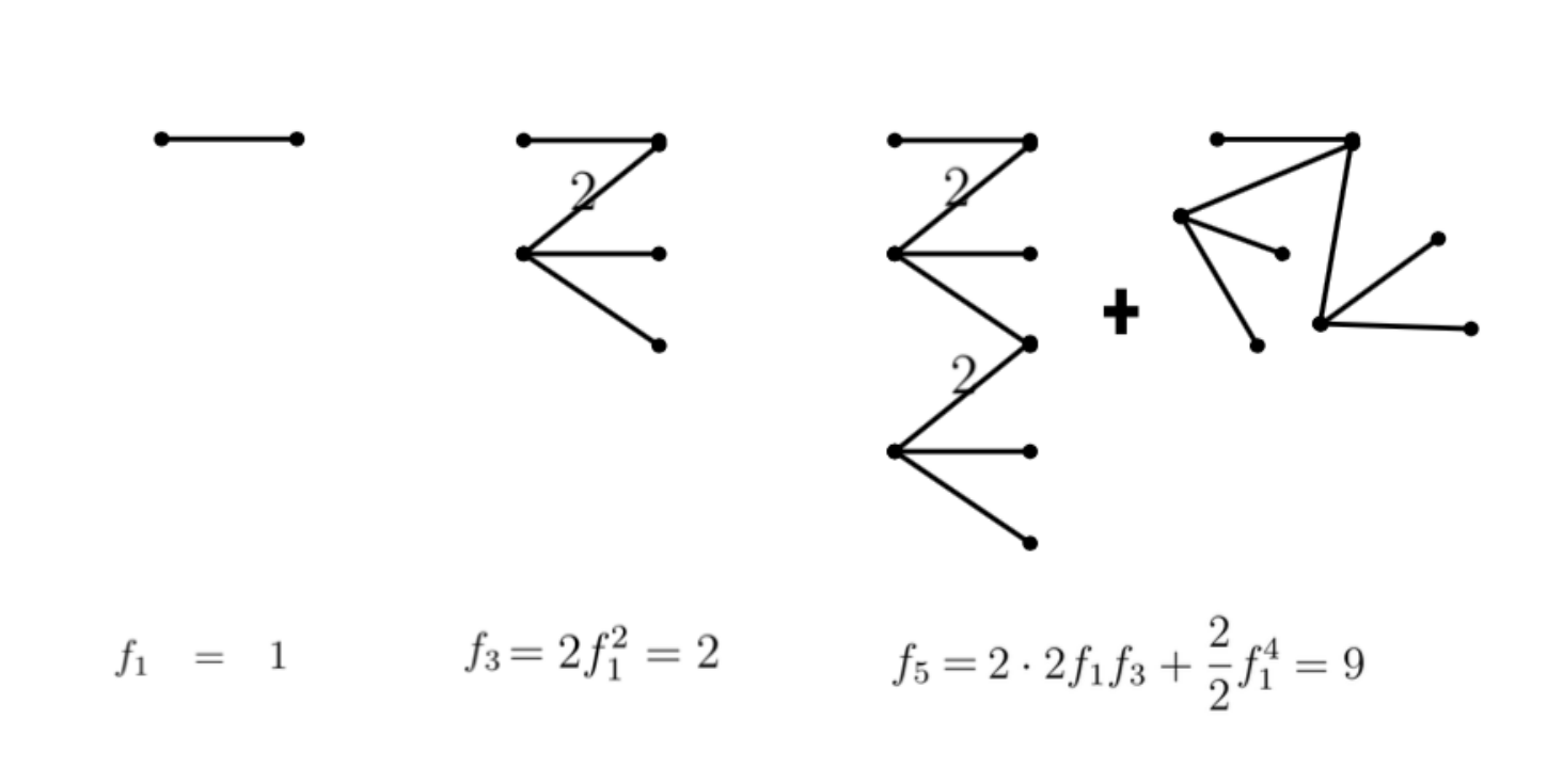
This procedure can be straightforwardly generalized to arbitrary $k$ and $d$ . If we denote $f_{n+1}^{k}$ by the number of contributing configuration with $n+1$ sink nodes, it can be obtained via following relation.

	$\displaystyle f^{k}_{n+1}$	$\displaystyle=$	$\displaystyle~{k-1\choose 1}\sum_{\begin{subarray}{c}a_{1},\cdots,a_{k-1}\\ \sum{a_{i}}=n\end{subarray}}f^{k}_{a_{1}}f^{k}_{a_{2}}\cdots f^{k}_{a_{k-1}}+{k-1\choose 2}\sum_{\begin{subarray}{c}a_{1},\cdots,a_{2(k-1)}\\ \sum{a_{i}}=n\end{subarray}}f^{k}_{a_{1}}f^{k}_{a_{2}}\cdots f^{k}_{a_{2(k-1)}}$		(3.13)
			$\displaystyle+\cdots+{k-1\choose k-1}\sum_{\begin{subarray}{c}a_{1},\cdots,a_{(k-1)^{2}}\\ \sum{a_{i}}=n\end{subarray}}f^{k}_{a_{1}}f^{k}_{a_{2}}\cdots f^{k}_{a_{(k-1)^{2}}}\ ,$		(3.13)

where the $i$ -th term counts the number of ways of attaching $i$ -many subquivers with $n$ sink nodes in total, to the initial quiver of type $(1,1)_{1}$ . Each subquiver can be further decomposed into an arrow (which is attached to the initial quiver) and $k-1$ sub-subquivers. When each of the latter contains $a_{p=1,\cdots k-1}$ -many sink nodes respectively, it contributes $f_{a_{p}}$ factor to the $i$ -th term. Finally, the combinatorial factor $k-1\choose i$ for $i$ -th term takes into account the number of ways of choosing flavor fugacity of arrows attached to the initial quiver, divided by order of the Weyl permutation of those.

Furthermore, this recursion relation can be neatly summarized by introducing the generating function

f_{k}(x)=\sum_{n=1}^{\infty}f^{k}_{n}x^{n}\ ,

(3.14)

with an auxiliary variable $x$ . Then the recursion relation (3.13) can be written in terms of the algebraic equation which (3.14) satisfies,

f_{k}(x)=x(1+f_{k}(x)^{(k-1)})^{(k-1)}\ .

(3.15)

Finally, the actual generating function of the quivers in question, i.e., the one obtained by gluing $d$ subquivers of type $(1,k)_{k}$ can be readily obtained in terms of $f_{k}(x)$ as

g_{k}(x)=f_{k}(x)^{k}\ ,

(3.16)

which takes into account the fact that the initial quiver has been replaced by $(1,k)_{k}$ quiver, yielding $k$ choices of initial gluing. Then $(k-1)d+1$ -th coefficient of $g_{k}$ encode the number of contributing arrows of quiver type $(d,(k-1)d+1)_{k}$ .

The coefficients of generating function which satisfies such algebraic equation can be evaluated by the Lagrange inversion theorem.[26, 37, 38] Especially, when a generating function satisfies an algebraic equation $f(x)=x(\phi(f(x))$ for a function $\phi(x)=1+ax^{b}$ , we have [26]

[x^{n}](f(x)))^{k}=\frac{k}{n}{n\choose\frac{n-k}{b}}a^{(n-k)/b}\ ,

(3.17)

where we denoted $[x^{n}]g(x)$ as $n$ -th coefficient of a power series $g(x)$ . Using this theorem, we can extract the general expression for the Witten index,

\Omega_{(d,(k-1)d+1)_{k}}=\frac{1}{d}~[x^{(k-1)d+1}]g_{k}(x)=\frac{k}{d((k-1)d+1)}{(k-1)^{2}d+(k-1)\choose d-1}\ .

(3.18)

Note that we further divided the answer by $d$ which corresponds to the choice of the initial quiver. The asymptotic behaviour of $d\rightarrow\infty$ for this expression can be also calculated, [26] which we can write as

\lim_{d\rightarrow\infty}\frac{\ln\Omega_{(d,(k-1)d+1)_{k}}}{d}=(k-1)^{2}\ln(k-1)^{2}-(k^{2}-2k)\ln(k^{2}-2k)\ .

(3.19)

Recently, it was noted by Galakhov et al. [28] that this exponentially large degeneracy of four-dimensional BPS states of conformal field theory is something unexpected, since the naive dimensional analysis implies a bound for the index, $\log|\Omega(E)|\leq aV^{1/4}E^{3/4}$ , where $E$ is energy of state supported in a finite volume $V$ . They showed that, by carefully examining Denef’s multi-center bound state formula [7], the radius of BPS bound state increases with the mass of the state. This corrects the above bound by $\log|\Omega(E)|\leq a^{\prime}E^{3/2}$ , which is consistent with the observed scaling behaviour of quiver quantum mechanics.

3.3 Mutation Equivalences

One of the most interesting properties of the 1d quiver quantum mechanics is that they are expected to be invariant under certain duality, which is called the mutation equivalence. In terms of the Kronecker quivers in question, it can be phrased into the isomorphism between moduli space of $(d_{1},d_{2})_{k}$ quiver with that of $(d_{2}k-d_{1},d_{2})_{k}$ , as shown in the Figure 3.

As a simple check, one can see the dimension of the classical moduli space of these two quivers are the same. Furthermore, we expect that, the equivariant indices of both quivers are the same, i.e.,

\Omega_{(d_{1},d_{2})_{k}}(y)=\Omega_{(d_{2},(k-1)d_{1}+1)_{k}}(y)\ ,

(3.20)

which is calculated for region $\zeta_{1}>0$ and $\zeta^{\prime}_{1}<0$ respectively. The index is trivially same for the other side of the wall, since both of them vanish. In particular, we will examine how the relation

\Omega_{(d,(k-1)d+1)_{k}}(y)=\Omega_{(d-1,d)_{k}}(y)

(3.21)

can be realized, using the diagrammatic expression of the JK residue developed so far.

Before delving into general $d$ and $k$ , we illustrate the proof of (3.21) for one of the simplest pair of the Kronecker quivers, $(2,3)_{3}$ and $(3,7)_{3}$ in detail, where the contributing charge sets are explicitly written down. In particular, we show that each fixed point determined by a set of hyperplane charges can be mapped to each other in a particular way.

Let us denote the Cartans of $(2,3)$ quiver by $u=(x_{1},x_{2},y_{1},y_{2},y_{3})$ . Then the equivariant index of this quiver can be written in the following expression

	$\displaystyle\Omega_{(2,3)}(y)$	$\displaystyle=$	$\displaystyle\text{JK-Res}_{\eta}~\frac{1}{2!}\frac{1}{3!}\left(\frac{1}{2\sinh[z/2]}\right)^{4}\left(\prod_{p\neq q}^{2}\frac{\sinh[(x_{p}-x_{q})/2]}{\sinh[(x_{p}-x_{q}-z)/2]}\right)$		(3.22)
			$\displaystyle\times\left(\prod_{k\neq l}^{3}\frac{\sinh[(y_{k}-y_{l})/2]}{\sinh[(y_{k}-y_{l}-z)/2]}\right)\prod_{p,k,i}\left(\frac{\sinh[(x_{p}-y_{k}-a_{i}-z)/2]}{\sinh[(x_{p}-y_{k}-a_{i})/2]}\right)\ ,\qquad$		(3.22)

where $a_{i}$ ’s are flavor fugacities for number of arrows. Since they potentially carry degenerate singularities, we need constructive definition of the JK-residue which can determine the ordered set of contributing charges. (For the definition used here, see [36] or section 2.4.3 of [33]). For this purpose, $\eta$ is chosen to be proportional to $\eta=(3,3,-2-\delta,-2,-2+\delta)$ with positive $\delta$ .^#4^#4 #4 In order to safely apply the constructive definition of the JK-residue explained in [36, 33], $\eta$ should not be at the boundary of flag defined by the sum of charges. Here, $\eta$ should be slightly shifted from $\zeta\sim(3,3,-2,-2,-2)$ since $\zeta$ can be spanned by $\sum_{i}Q_{i}$ , sum of all charge sets. If we carefully examine the JK-condition with this choice of $\eta$ , it turns out that the following ordered set of charges passes the JK condition, and potentially non-zero.

	$\displaystyle x_{1}-y_{1}-a_{i_{1}}$
	$\displaystyle x_{2}-y_{2}-a_{i_{2}}$
	$\displaystyle x_{2}-y_{3}-a_{i_{3}}$
	$\displaystyle x_{1}-y_{2}-a_{i_{4}}\ ,$		(3.23)

with their Weyl copies $x_{1}\leftrightarrow x_{2}$ and all different different set of flavor fugacities. When $a_{i_{1}}\neq a_{i_{4}}$ , $a_{i_{2}}\neq a_{i_{3}}$ and $a_{i_{2}}\neq a_{i_{4}}$ , this singularity is non-degenerate. On the other hand, if $a_{i_{2}}=a_{i_{4}}$ , this singularity becomes degenerate which has two additional poles $x_{1}-y_{3}-a_{i_{3}}$ , $x_{2}-y_{1}-a_{i_{1}}$ and order two zero from $x_{1}=x_{2}$ .^#5^#5 #5 For the latter case, the order of $y_{1},y_{2},y_{3}$ ’s are fixed by choice of the sign of $\delta$ . Other than these, the residue integral vanish due to the zero’s of vector multiplet. These two different classes of singularities are illustrated in the second and the fourth diagram of Figure 4 respectively.

Meanwhile, the equivariant index of $(3,7)$ quiver with three arrows can be obtained from gluing three $(1,3)_{3}$ quivers as was shown in the last section. It turns out that there are two topologically distinguished contributing arrows which can be obtained. These are also illustrated in the first and the third diagram of Figure 4. The non-equivariant index can be evaluated simply by counting number of ways of assigning flavor fugacities to each arrows up to symmetries of diagram. This turns out to be $-12$ and $-1$ respectively.

Interestingly, one can show that these two types of diagrams are mapped respectively to the two different types of fixed points of the $(2,3)$ quiver. For this purpose, we rewrite a term in the integral in (3.22) evaluated at (3.23) with $a_{i_{1}}=a_{1},a_{i_{2}}=a_{2},a_{i_{3}}=a_{1},a_{i_{4}}=a_{3}$ as follow,

	$\displaystyle~\frac{1}{2!}\frac{1}{3!}\left(\frac{1}{2\sinh[z/2]}\right)^{4}\oint_{y_{1}=y_{2}+a_{3}-a_{1}}\oint_{y_{3}=y_{2}+a_{2}-a_{1}}\left(\prod_{k\neq l}^{3}\frac{\sinh[(y_{k}-y_{l})/2]}{\sinh[(y_{k}-y_{l}-z)/2]}\right)$
	$\displaystyle\oint_{x_{2}=y_{2}+a_{2}}\oint_{x_{1}=y_{1}+a_{1}}\left(\prod_{p\neq q}^{2}\frac{\sinh[(x_{p}-x_{q})/2]}{\sinh[(x_{p}-x_{q}-z)/2]}\right)\prod_{p,k,i}\left(\frac{\sinh[(x_{p}-y_{k}-a_{i}-z)/2]}{\sinh[(x_{p}-y_{k}-a_{i})/2]}\right).~~\qquad$		(3.24)

Note that, the integral over all $x_{i}$ ’s in the last line can be evaluated to the simple expression as

2!\cdot(2\sinh[z/2])^{2}\prod_{\begin{subarray}{c}y_{i},a_{i}\in A\\ y_{j},a_{j}\in A^{\prime}\end{subarray}}\frac{\sinh[(y_{i}-y_{j}+a_{i}-a_{j}-z)/2]}{\sinh[(y_{i}-y_{j}+a_{i}-a_{j})/2]}\ .

(3.25)

Here we defined that $A$ is a subset of all combinations $y_{i}+a_{i}$ which is integrated over in the above integral (this case $y_{1}+a_{1}$ and $y_{2}+a_{2}$ ), and $A^{\prime}$ is the complement of $A$ in which case we have 7 elements. The factor $2!$ takes into account the Weyl equivariant singular point.

On the other hand, if we look at $(3,7)$ quiver side, we have

	$\displaystyle\Omega_{(3,7)}(y)$	$\displaystyle=$	$\displaystyle-\text{JK-Res}_{\eta^{\prime}}~\frac{1}{7!}\frac{1}{3!}\left(\frac{1}{2\sinh[z/2]}\right)^{9}\left(\prod_{p\neq q}^{7}\frac{\sinh[(\tilde{x}_{p}-\tilde{x}_{q})/2]}{\sinh[(\tilde{x}_{p}-\tilde{x}_{q}-z)/2]}\right)$		(3.26)
			$\displaystyle\times\left(\prod_{k\neq l}^{3}\frac{\sinh[(y_{k}-y_{l})/2]}{\sinh[(y_{k}-y_{l}-z)/2]}\right)\prod_{p,k,i}\left(\frac{\sinh[(-\tilde{x}_{p}+y_{k}+a_{i}-z)/2]}{\sinh[(-\tilde{x}_{p}+y_{k}+a_{i})/2]}\right)\ .\qquad$		(3.26)

Since all the poles are all non-degenerate, we can safely change the order of integration without affecting the result. Suppose that we have contributing arrows defined by the following assignments of flavor fugacities, and fix the integration order as specified below.

	$\displaystyle-\tilde{x}_{1}+y_{1}+a_{3}$
	$\displaystyle-\tilde{x}_{2}+y_{1}+a_{2}$
	$\displaystyle-\tilde{x}_{3}+y_{2}+a_{3}$
	$\displaystyle-\tilde{x}_{4}+y_{2}+a_{1}$
	$\displaystyle-\tilde{x}_{5}+y_{3}+a_{1}$
	$\displaystyle-\tilde{x}_{6}+y_{3}+a_{2}$
	$\displaystyle-\tilde{x}_{7}+y_{3}+a_{3}$
	$\displaystyle-\tilde{x}_{3}+y_{1}+a_{1}$
	$\displaystyle-\tilde{x}_{5}+y_{2}+a_{2}$

If we evaluate the residue integral for the first seven poles, it yields a factor

7!\cdot(\sinh[z/2])^{7}\prod_{\begin{subarray}{c}y_{i},a_{i}\in A\\ y_{j},a_{j}\in A^{\prime}\end{subarray}}\frac{\sinh[(y_{i}-y_{j}+a_{i}-a_{j}-z)/2]}{\sinh[(y_{i}-y_{j}+a_{i}-a_{j})/2]}\ ,

(3.27)

where the sets $A$ and $A^{\prime}$ are exactly the same as what is defined in the expression (3.25). Again, we have a factor of $7!$ which takes into account different fixed points obtained by the Weyl permutation of $\tilde{x}_{i}^{\prime}s$ . In this way, for a given set of charges of $(2,3)$ quiver which satisfies the JK condition, we get unique rank 9 singularity for $(3,7)$ quiver after summing over the Weyl permutations for both sides, and vice versa. Note that for charge sets mapped like this, we are left with exactly the same integral over non-mutated nodes. This procedure is summarised in Figure 5. Summing over all contributions, we end up with

\Omega_{(3,7)_{3}}(y)=\Omega_{(2,3)_{3}}(y)=-\frac{1}{{\bf y}^{6}}-\frac{1}{{\bf y}^{4}}-\frac{3}{{\bf y}^{2}}-3-3{\bf y}^{2}-{\bf y}^{4}-{\bf y}^{6}\ ,

(3.28)

which agrees with the formula obtained in various literatures. [30, 15, 25]

If we look at Figure 4 where we illustrated the mapping of each contributing arrows, it is interesting to note that the contributing arrows of $(2,3)_{3}$ quivers appear as a subdiagram of contributing arrows of its mutation dual quiver. Once we pick all the arrows directly attached to the glued nodes, it gives a unique diagram which corresponds to the contributing arrows of the dual quiver which has the same residue integral.

As can be seen in this example, once we classify all contributing arrows of both side of the dual pair, this procedure may be generalised to arbitrary $d$ and $k$ . Suppose that, there exist an ordered charge set $\{Q_{i}\}$ which satisfies the JK-condition for the $(d,(k-1)d+1)_{k}$ quiver. Since this is non-degenerate, we can choose an order of the charge set in a way that we could integrate over all $\tilde{x}_{i}$ ’s first, as was shown in the example. Given this set, we uniquely pick a subquiver which includes all the arrows directly connected to the glued node. Out of this subquiver, we associate a unique bipartite quiver as in Figure 4, with flavor fugacities assigned. One can easily check that bipartite diagrams are the only possibility which satisfies the JK-condition with $r=2d-2$ charges for $(d-1,d)_{k}$ quiver. Then, for non-degenerate poles of the latter, it is a direct generalization of the above example that the residue of this pole is the same as that of a pole of the original quiver. For degenerate poles of $(d-1,d)_{k}$ quivers, it needs to be separatley confirmed that the poles which can be obtained this way saturate all set of degenerate poles of the dual quiver, after shifting FI parameter properly as in the above example.

4 Comments

To conclude, we would like to mention several interesting questions which follows immediately.

1.

From the residue integral expression, we can systematically obtain the index for the Kronecker quiver with non-coprime dimension vector. It would be interesting to study the scaling behaviour for non-coprime charges $\Omega((n,n)_{k})$ directly. As was partly shown in the Appendix, this type of quivers always involve particular contributing charge sets which contain poles in the vector multiplet. This implies that the index gets contribution from the flat direction in the Coulomb branch, which can be inferred from the fact that we generally get the fractional number for the poles of such type.
2.

One of the most interesting problem remaining is to find a large-rank scaling behaviour of quivers with oriented loop, which is closely related to counting the degeneracy of the single centered BPS black hole in four-dimensional ${\cal N}=2$ theory. It would be interesting to see if we can find any quiver with loop whose large-rank behaviour is accessible through the residue integral formula.
3.

The index formula described in this note is given by particular sum over various residue integrals, and the formula described by MPS [14, 15] and Reineke [30] are also written in terms of sum of various partitions. It would be interesting to see how our construction is related to the latter two expansion. One of the pros of using the residue integral definition is that it is rather easy to see the large rank behaviour and the mutation equivalence of quivers, as shown in the example of the last section. It remains to check if mutation equivalence holds for other types of the tree-like quiver and quiver with loops.

Acknowledgement

The author is grateful to Piljin Yi for fruitful comments and reviewing the manuscript, and thanks to Seung-Joo Lee for useful discussion. The research was supported by the Perimeter Institute for Theoretical Physics. Research at Perimeter Institute is supported by the Government of Canada through Industry Canada and by the Province of Ontario through the Ministry of Economic Development and Innovation. This research was made possible through the support of a grant from John Templeton Foundation. The opinions expressed in this publication are those of the author and do not necessarily reflect the views of the John Templeton Foundation.

Appendix A Technical Details

For quivers of type $(d_{1},d_{2})_{1}$ , vector multiplet does not contribute when $d_{1}\neq d_{2}$ .

Proof. Suppose that there exist a co-dimension $r$ singularity which contains poles from vector multiplet $x_{i}-x_{j}=z$ . Then since $\eta$ is taken to be positive for the first node, it should be followed by a pole of type $x_{j}-x_{k}=z$ or $x_{j}-y_{k}=0$ . Since a charge set without any chiral multiplet cannot generate rank $r$ singularity, we need at least one pole from the chiral multiplet. Thus in general, poles that contain vector multipets have a sequence

x_{i_{1}}-x_{i_{2}}=z,~x_{i_{2}}-x_{i_{3}}=z,\cdots,x_{i_{k}}-x_{j}=z,~x_{j}-y_{l}=0

(A.1)

as a part. However the last two relations generate the equation $x_{i_{k}}-y_{l}-z=0$ which is zero of the hypermultiplet, and the only possibility that a pole involving vector multiplet contributes is that additional poles collide and become degenerate. Let us scan all the charges possibly connected to this set. For $y_{p_{1}}\neq y_{l}$ ,

1)

$y_{l}-y_{p_{1}}=z$ : generates additional zero $x_{j}-y_{p_{1}}-z=0$ .
2)

$y_{p_{1}}-y_{l}=z$ : gives additional pole $x_{i_{k}}-y_{p_{1}}=0$ .
3)

$x_{i_{0}}-y_{l}=0$ : gives order two zero from $x_{i_{0}}-x_{j}=0$ .
4)

$x_{i_{0}}-x_{i_{a}}=\pm z$ : generates order two zero or go back to the same type.
5)

$x_{j}-y_{p_{1}}=0$ : yields order two zero from $y_{l}-y_{p_{1}}=0$ .
6)

$x_{i_{1}}-y_{p_{1}}=0$ : No additional poles or zero.
7)

$x_{i_{a}}-y_{p_{1}}=0$ : additional zero from $x_{i_{a-1}}-y_{p_{1}}=z$ .

From these possibilities, we see that the sequences (A.1) can contribute only when it also contains a pole of type $y_{p_{1}}-y_{l}=z$ . However when $k>1$ , introducing this pole yields another relation $x_{i_{k-1}}-y_{p_{1}}=z$ which generates a zero. In order to cancel this zero again, we further introduce $y_{{p_{2}}}-y_{p_{1}}=z$ in a similar manner. This procedure continues to introduce $k$ additional $y_{p}$ ’s, and we end up with the relations

	$\displaystyle x_{i_{1}}-x_{i_{2}}=z,~x_{i_{2}}-x_{i_{3}}=z,\cdots,x_{i_{k}}-x_{j}=z\ ,$
	$\displaystyle y_{p_{k}}-y_{p_{k-1}}=z,~y_{p_{k-1}}-y_{p_{k-2}}=z,\cdots,y_{p_{1}}-y_{l}=z\ ,$
	$\displaystyle x_{j}=y_{l},~x_{i_{k}}=y_{p_{1}},\cdots,x_{i_{2}}=y_{p_{k-1}},~x_{i_{1}}=y_{p_{k}},$		(A.2)

which involves exactly $k+1$ pairs of $x$ ’s and $y$ ’s. If we try to add one more cartan $y_{k+1}$ which is related to the above set by adding $x_{i_{a}}-y_{k+1}=0$ or $y_{p_{a}}-y_{k+1}=z$ , it always generates additional zeros of type $y_{p_{k+1-a}}-y_{k+1}=0$ or $x_{i_{k+1-a}}-y_{k+1}=z$ . Finally, if we add $y_{k+2}-y_{i}=z$ , this goes back to the argument of the beginning, again introduces new $x_{i_{k+1}}$ which falls into type (A.2). Hence the set cannot be connected to other Cartans by adding additional poles. However, when $d_{1}\neq d_{2}$ , one can see that the singularity involving this set cannot meet the JK condition. This is simply because, sum of all components of any linear combination $\sum_{i}a_{i}Q_{i}$ vanishes where $Q_{i}$ ’s are charge sets appearing in (A.2). The analysis implies that the vector multiplet cannot contributes for co-prime $d_{1}$ and $d_{2}$ , but they can contribute if $d_{1}=d_{2}$ , even for larger intersection number $k$ .

A2

Consider a quiver with type $(d,(k-1)d+1)_{k}$ and their particular set of $r=kd$ contributing arrows. In this set, for each $i\in I$ , there are exactly $k$ arrows of type $x_{i}-y_{j}-a_{\alpha}$ .

Proof. Note that the rank of this quiver is $kd$ . In order to satisfy the JK condition, there must exist a set of $kd$ positive coefficients $a_{i,j,\alpha}$ , such that

$\zeta=\sum a_{i,j,\alpha}Q_{i,j,\alpha}=((m-1)d+1,\cdots,(m-1)d+1,-d,\cdots,-d)$ (A.3)

holds. Here $Q_{i,j,\alpha}$ denotes a charge vector which gives a pole of type $x_{i}-y_{j}-a_{\alpha}$ . Now suppose that there exist $i\in I$ such that there are $m-q$ (for $0<q<m$ ) charges of a form $x_{i}-y_{j_{p}}-a_{\alpha}$ . Then there is at least one $j_{0}$ such that $a_{i,j_{0},a}$ , the coefficient for charge of type $x_{i}-y_{j}-a_{\alpha}$ , satisfies

$a_{i,j_{0},\alpha}>\frac{(m-1)d+1}{m-q}>d.$ (A.4)

Then it is clear that existence of the coefficient of this property violates $j_{0}$ -th component of the equation (A.3). Hence, for each $i$ , there should be at least $k$ vectors of type $x_{i}-y_{j_{p}}-a_{\alpha}$ . Furthermore, since the number of charges are exactly $kd$ , we can say that there should be exactly $k$ charges of type $x_{i}-y_{j_{p}}-a_{\alpha}$ for each $i$ .
A3

1) For quivers with dimension vector $(d,(k-1)d+1)$ , degenerate poles do not contribute to the index.

2) Suppose that there exist two charges $x_{i}-y_{j}-a_{\alpha}$ and $x_{i}-y_{j}^{\prime}-a_{\beta}$ with $a_{\alpha}=a_{\beta}$ , for any $i$ in a contributing arrow set. Then this set does not contribute to the integral. Similarly, for a sink node $j$ , if there exist two charges $x_{i}^{\prime}-y_{j}-a_{\alpha}$ and $x_{i}-y_{j}-a_{\beta}$ with $a_{\alpha}=a_{\beta}$ , this set does note contribute to the integral.

Proof. For non-degenerate singularities, poles of type 2) do not contribute due to the zeros of the vector multiplets. However, these singularities may contribute for degenerate singularities because of additional pole orders. Note that, since the rank of the gauge group is $kd$ and there are only $k$ flavors, degenerate singularity can appear only when one of the 2) is satisfied.

Let us briefly summarise how we can deal with such singularities in general. Consider a gauge group with rank $r$ . Then the JK residue gets contribution from codimension $r$ -singularities defined by

$Q_{i}\cdot u=0\ ,$ (A.5)

for $i=1,\dots s$ with $s\geq r$ . When $s=r$ , definition of the JK residue integral can be unambiguously written down as (3.1). On the other hand, for $s>r$ , which we call degenerate singularity, the final answer depends very much on the order of taking residues, and we need an alternative definition of JK residue which clarifies this ambiguity. In the literature, there exist several equivalent definitions which could be applied for these type of singularities. [33, 34, 35, 36] Among them, we are going to use the definition elaborated in [35, 39], which we briefly summarize as below.

Suppose that we have rank $r$ degenerate singularity with charges $\{Q_{i=1,\cdots p}\}$ with $p\geq r$ colliding. From these, we fix the order of charges arbitrary, and denote this ordered set as $\Delta=\{Q_{1},\cdots Q_{p}\}$ . Among them, there are ${}_{p}C_{r}$ choices of picking up an ordered set with $r$ -entry, which we denote as $b=\{Q_{i_{1}},\cdots Q_{i_{r}}\}$ . Finally, for each $b$ , we assign so called basic fraction,

$\phi_{b}=\frac{1}{(Q_{i_{1}}\cdot u)\cdots(Q_{i_{r}}\cdot u)}\ .$ (A.6)

Out of these basic fraction $\phi_{b}$ ’s, we can build a set $b\in B$ such that $B$ form a rank $r$ basis of the basic fractions. Then, from $B$ , one can obtain any meromorphic function in $u$ -plane by taking derivatives and linear combinations of elements in $\phi_{b\in B}$ .

Furthermore, the useful fact is that, for any choice of ordering of set $\Delta$ , we can find a set $B$ such that we can define iterated residue,

$\text{Iterated-Res}_{b\in B}:=\text{Res}_{Q_{i_{r}}\cdot u=0}\cdots\text{Res}_{Q_{i_{1}}\cdot u=0}$ (A.7)

with $b=\{Q_{i_{1}},\cdots Q_{i_{r}}\}$ , which satisfy

$\text{Iterated-Res}_{b\in B}~\phi_{b^{\prime}}=\delta_{bb^{\prime}}\ .$ (A.8)

In particular, RHS of the definition (A.7) should be regarded as iterated operation of the residue integral from the rightmost one, keeping other components of $u$ at generic points. With all these definitions, JK-residue for this degenerate point can be simply written as

$\text{JK-Res}(\eta,\{Q_{1},\cdots,Q_{p}\})=\sum_{b\in B,~\eta\in\text{Cone}(b)}\nu(b)~\text{Iterated-Res}_{b}\ ,$ (A.9)

where $\nu(b)=$ sgn(det $b$ ). With this alternative definition of the JK-residue, we are going to show that for quiver with type $(d,(k-1)d+1)_{k}$ , there is no degenerate point which contributes to the integral.
As was mentioned above, for the Kronecker quivers of this type, degenerate singularities from chiral multiplets can appear only when one of the following is satisfied.
- 1.
  
  Contributing arrows contain two charges $x_{i}-y_{j}-a_{\alpha}$ and $x_{i}-y_{j^{\prime}}-a_{\beta}$ such that $a_{\alpha}=a_{\beta}$ .
- 2.
  
  Contributing arrows contain two charges $x_{i}-y_{j}-a_{\alpha}$ and $x_{i^{\prime}}-y_{j}-a_{\beta}$ such that $a_{\alpha}=a_{\beta}$ .
First, let us consider the first case. Suppose that there exist such $i\in I$ and $j,j^{\prime}\in J$ . If both of $j,j^{\prime}$ are not connected to any other source nodes, then this pole can be non-degenerate, but they do not contribute since they generate the relation $y_{j}=y_{j^{\prime}}$ , which introduces order 2 zero from the vector multiplet numerator. If there exist charges of type $x_{i^{\prime}}-y_{j}-a_{\gamma}$ or $x_{i^{\prime\prime}}-y_{j^{\prime}}-a_{\delta}$ in this charge set, they generate additional relations $x_{i^{\prime}}-y_{j^{\prime}}-a_{\gamma}$ or $x_{i^{\prime\prime}}-y_{j}-a_{\delta}$ . This implies that the corresponding pole additionally collides at the singular point, so the singularity become degenerate.
Let us consider the second possibility. Suppose that we have such $i,i^{\prime}\in I$ and $j\in J$ in a given set of contributing arrows. It is rather easy to show that the second type of degenerate points never contribute even if they generate degeneracy. Suppose that there exist such $j\in J$ and $i,i^{\prime}\in I$ which are assigned to a same flavor charge. Then from the argument of A2, we know that there exist at least $k-1$ $j^{\prime}$ which is connected to $i$ -th source node by $x_{i}-y_{j^{\prime}}-e_{\gamma}$ , and $k-1$ $j^{\prime\prime}$ which is connected to $i^{\prime}$ -th source node by $x_{i^{\prime}}-y_{j^{\prime\prime}}-e_{\delta}$ . Then they generate $k-1$ additional relations of type $x_{i^{\prime}}-y_{j^{\prime}}-e_{\gamma}=0$ , and also the additional $k-1$ relations of type $x_{i}-y_{j^{\prime\prime}}-e_{\delta}=0$ . In total, there are $2(k-1)$ additional poles which additionally collide at this singular point. However, they also generate at least $2(k-1)$ zeros of type $y_{j_{a}}=y_{j_{b}}$ for $a\neq b$ and two more from $x_{i}=x_{i^{\prime}}$ . Since the order of additional zero $(2k)$ always exceeds additional pole $(2(k-1))$ , this degenerate singularity never contributes.
Finally, let us come back to the first degenerate singularity. Suppose that $y_{j}=y_{j}^{\prime}$ is the only relation which gives additional zero. Note that, for this case, there may exist a singularity where number of additional poles exceed or equal to the number of additional zeros. However, one can show that they never satisfy the JK-condition. First of all, since we have a freedom to choose the order of the charge set, we set the order of charges $\Delta$ such that $x_{i}-y_{j}-a_{\alpha}$ $(:=Q_{1})$ appear at the very first position, and immediately followed by $x_{i}-y_{j^{\prime}}-a_{\alpha}$ $(:=Q_{2})$ . Then the ordered set $b$ contained in the set $B$ constructed as above procedure should be one of the following.
- 1)
  
  $\{Q_{1},Q_{2},\cdots\}$
- 2)
  
  $\{Q_{1},Q_{i_{1}},\cdots\}$
- 3)
  
  $\{Q_{2},Q_{i_{2}},\cdots\}$
- 4)
  
  $\{Q_{i_{2}},\cdots\}$
where $Q_{i_{1,2}}\neq Q_{1}\text{ or }Q_{2}$ . Note that the case $1)$ has residue zero since this relation imposes $y_{j}=y_{j^{\prime}}$ which gives arise the order two zero. There are no additional poles at this point since the other components of $u$ are kept generic, by the definition of the iterated residue. Finally, consider the second, third and the fourth case. If the set $b$ still has $k$ arrows connected to the source $x_{i}$ , then it defines rank $kd$ equation without any additional relations. If this is the case, the relation imposed by the original set $\Delta$ would have been overdetermined and cannot define a singularity. Hence, we can conclude that there are less than $k$ arrows emerging from source $x_{i}$ in the set $b$ of type 2),3) and 4). Going back to the proof of A2, we concluded that this type of charge set $b$ cannot satisfy the JK condition. This procedure straightforwardly generalizes to the charge sets with larger number of additional zeros.

All configurations of contributing arrows obtained from gluing that of $(1,k)_{k}$ quiver satisfy the JK condition.

Proof. This can be proven by induction. First, let us assume that the statement is true for $(d,(k-1)d+1)_{k}$ type quiver. It means that we have a set of $kd$ positive coefficients $a_{i,j,\alpha}$ such that the relation

\zeta_{d}=((k-1)d+1,\cdots,(k-1)d+1,-d,\cdots,-d)=\sum a_{i,j,\alpha}Q_{i,j,\alpha}

(A.10)

holds, where $\{Q_{i,j,\alpha}\}$ is a charge set with $kd$ elements which is obtained from the gluing procedure. The assignment of flavor symmetry $\alpha$ obeys the two conditions in 2) of A3. Now, we attach a subquiver of type $(1,m)$ to this quiver by identifying one of the sink node $y_{j}$ of the original quiver with that of new subquiver $y_{j^{\prime}}$ by $j=j^{\prime}=j_{0}$ . We will see that for all such possible gluing, there exists a positive coefficient set $\{a^{\prime}_{i,j,\alpha}\}$ with $k(d+1)$ elements such that it satisfies

\zeta_{d+1}=((k-1)(d+1)+1,\cdots,(k-1)(d+1)+1,-d-1,\cdots,-d-1)=\sum_{i,j\in A^{\prime}}a^{\prime}_{i,j,\alpha}Q^{\prime}_{i,j,\alpha}\ ,

(A.11)

where $Q^{\prime}_{i,j,\alpha}$ is a charge of the new quiver. We can show that positive coefficient $a_{i,j,\alpha}^{\prime}$ that satisfies (A.11) can be easily constructed from $a_{i,j,\alpha}$ of the original quiver. Here, we denoted $A$ as a set of all nodes of original quiver of type $(d,(k-1)d+1)_{k}$ , and $A^{\prime}$ as a set of all nodes of new quiver $(d+1,(k-1)(d+1)+1)_{k}$ . First of all, $a^{\prime}_{i,j,\alpha}$ , with $i,j\in A^{\prime}\backslash A$ , (i.e., when $i=d+1$ ) can be uniquely identified as $a^{\prime}_{d+1,j\neq j_{0},\alpha}=d+1$ . Then it follows that $a^{\prime}_{d+1,j_{0},\alpha}=1$ . Since all the arrows are connected, we can define numbers $a^{\prime}_{i,j,\alpha}$ for all $i,j\in A$ through the following procedure. First of all, consider the $j_{0}$ -th component of the above equation. Since $a^{\prime}_{i,j_{0},\alpha}$ satisfies $\sum_{i,}a^{\prime}_{i,j_{0},\alpha}=d+1$ and $a^{\prime}_{d+1,j_{0},\alpha}=1$ , we can set $a^{\prime}_{i,j_{0},\alpha}=a_{i,j_{0},\alpha}$ for all $i\neq d+1$ . Then, consider $a_{i,j,\alpha}$ ’s for the above $i$ ’s and $j\neq j_{0}$ . If we look at $i$ -th components of the equation, they imply $a^{\prime}_{i,j^{\prime},\alpha}=a_{i,j^{\prime},\alpha}+1$ with $j^{\prime}\neq j_{0}$ . Next, consider the $j^{\prime}$ -th component of the equation. Similarly, this implies that $a^{\prime}_{i^{\prime},j^{\prime\prime},\alpha}=a_{i^{\prime},j^{\prime\prime},\alpha}$ for all $j^{\prime\prime}\neq j^{\prime}$ . We can continue this procedure until all $a^{\prime}$ ’s are specified. Since there is no cycle and every nodes are connected, this procedure can uniquely fix all the coefficients $a^{\prime}_{i,j,\alpha}$ which are by construction all positive. Finally, since the statement obvious holds for $d=1$ , we can say that for all $d$ , $(d,(k-1)d+1)_{k}$ type quiver obtained from the gluing method satisfy the JK condition.

References

[1] N. Seiberg and E. Witten, “Electric - magnetic duality, monopole condensation, and confinement in N=2 supersymmetric Yang-Mills theory,” Nucl. Phys. B 426 (1994) 19 [Erratum-ibid. B 430 (1994) 485] [hep-th/9407087].
[2] N. Seiberg and E. Witten, “Monopoles, duality and chiral symmetry breaking in N=2 supersymmetric QCD,” Nucl. Phys. B 431 (1994) 484 [hep-th/9408099].
[3] F. Ferrari and A. Bilal, “The Strong coupling spectrum of the Seiberg-Witten theory,” Nucl. Phys. B 469 (1996) 387 [hep-th/9602082].
[4] K. -M. Lee and P. Yi, “Dyons in N=4 supersymmetric theories and three pronged strings,” Phys. Rev. D 58, 066005 (1998) [hep-th/9804174].
[5] M. R. Douglas, B. Fiol and C. Romelsberger, “Stability and BPS branes,” JHEP 0509 (2005) 006 [hep-th/0002037].
[6] M. R. Douglas, B. Fiol and C. Romelsberger, “The Spectrum of BPS branes on a noncompact Calabi-Yau,” JHEP 0509 (2005) 057 [hep-th/0003263].
[7] F. Denef, “Quantum quivers and Hall / hole halos,” JHEP 0210 (2002) 023 [hep-th/0206072].
[8] F. Denef and G. W. Moore, “Split states, entropy enigmas, holes and halos,” JHEP 1111 (2011) 129 [hep-th/0702146 [HEP-TH]].
[9] M. Kontsevich and Y. Soibelman, “Stability structures, motivic Donaldson-Thomas invariants and cluster transformations,” [arXiv:0811.2435]
[10] D. Gaiotto, G. W. Moore and A. Neitzke, “Four-dimensional wall-crossing via three-dimensional field theory,” Commun. Math. Phys. 299 (2010) 163 [arXiv:0807.4723 [hep-th]].
[11] D. Gaiotto, G. W. Moore and A. Neitzke, “Wall-crossing, Hitchin Systems, and the WKB approximation,” arXiv:0907.3987 [hep-th].
[12] D. Gaiotto, G. W. Moore and A. Neitzke, “Framed BPS states,” arXiv:1006.0146 [hep-th].
[13] J. de Boer, S. El-Showk, I. Messamah and D. Van den Bleeken, “Quantizing N=2 multicenter solutions,” JHEP 0905 (2009) 002 [arXiv:0807.4556 [hep-th]].
[14] J. Manschot, B. Pioline and A. Sen, “Wall crossing from Boltzmann black hole halos,” JHEP 1107, 059 (2011) [arXiv:1011.1258 [hep-th]].
[15] J. Manschot, B. Pioline and A. Sen, “A Fixed point formula for the index of multi-centered N=2 black holes,” JHEP 1105, 057 (2011) [arXiv:1103.1887 [hep-th]].
[16] H. Kim, J. Park, Z. Wang and P. Yi, “Ab initio wall-crossing,” JHEP 1109, 079 (2011) [arXiv:1107.0723 [hep-th]].
[17] A. Sen, “Equivalence of three wall-crossing formulae,” Commun. Num. Theor. Phys. 6, 601 (2012) [arXiv:1112.2515 [hep-th]].
[18] J. Manschot, B. Pioline and A. Sen, “On the Coulomb and Higgs branch formulae for multi-centered black holes and quiver invariants,” JHEP 1305, 166 (2013) [arXiv:1302.5498 [hep-th]].
[19] J. Manschot, B. Pioline and A. Sen, “The Coulomb branch formula for quiver moduli spaces,” arXiv:1404.7154 [hep-th].
[20] K. Hori, H. Kim and P. Yi, “Witten Index and Wall Crossing,” JHEP 1501 (2015) 124 [arXiv:1407.2567 [hep-th]].
[21] C. Cordova and S. -H. Shao, “An index formula for supersymmetric quantum mechanics,” arXiv:1406.7853 [hep-th].
[22] C. Cordova and S. H. Shao, “Asymptotics of Ground State Degeneracies in Quiver Quantum Mechanics,” arXiv:1503.03178 [hep-th].
[23] C. Hwang, J. Kim, S. Kim and J. Park, “General instanton counting and 5d SCFT,” arXiv:1406.6793 [hep-th].
[24] B. Kol, “Thermal monopoles,” JHEP 0007 (2000) 026 [hep-th/9812021].
[25] K. Ohta and Y. Sasai, JHEP 1411 (2014) 123 [arXiv:1408.0582 [hep-th]].
[26] Weist, Thorsten. ”Localization in quiver moduli spaces.” Representation Theory of the American Mathematical Society 17.13 (2013): 382-425.
[27] Weist, Thorsten. ”On the Euler characteristic of Kronecker moduli spaces.” Journal of Algebraic Combinatorics 38.3 (2013): 567-583.
[28] D. Galakhov, P. Longhi, T. Mainiero, G. W. Moore and A. Neitzke, “Wild Wall Crossing and BPS Giants,” JHEP 1311 (2013) 046 [arXiv:1305.5454 [hep-th]].
[29] C. Cordova and S. H. Shao, “Counting Trees in Supersymmetric Quantum Mechanics,” arXiv:1502.08050 [hep-th].
[30] M. Reineke, “The Harder-Narasimhan system in quantum groups and cohomology of quiver moduli,” Invent. Math. 152 (2003) 349-368; arXiv:math/0204059 [math.QA].
[31] M. Alim, S. Cecotti, C. Cordova, S. Espahbodi, A. Rastogi and C. Vafa, “BPS Quivers and Spectra of Complete N=2 Quantum Field Theories,” Commun. Math. Phys. 323 (2013) 1185 [arXiv:1109.4941 [hep-th]].
[32] M. Alim, S. Cecotti, C. Cordova, S. Espahbodi, A. Rastogi and C. Vafa, “ $\mathcal{N}=2$ quantum field theories and their BPS quivers,” Adv. Theor. Math. Phys. 18 (2014) 27 [arXiv:1112.3984 [hep-th]].
[33] F. Benini, R. Eager, K. Hori and Y. Tachikawa, “Elliptic Genera of 2d ${\mathcal{N}}$ = 2 Gauge Theories,” Commun. Math. Phys. 333 (2015) 3, 1241 [arXiv:1308.4896 [hep-th]].
[34] L. C. Jeffrey and F. C. Kirwan, “Localization for nonabelian group actions,” Topology 34 (1995) 291-327, arXiv:alg-geom/9307001.
[35] M. Brion and M. Vergne, “Arrangement og hyperplanes I: Rational functions and Jeffrey-Kirwan residue,” Ann. Sci. ENS 32 (1999) 715-741, arXiv:math/9903178 [math.DG].
[36] A. Szenes and M. Vergne, “Toric reduction and a conjecture of batyrev and materov,” Invent. Math. 158 (2004) 453-495, arXiv:math/0306311 [math.AT].
[37] Sedgewick, R., Flajolet, P., “An Introduction to the Analysis of Algorithms”, Addison Wesley, 1996
[38] Drmota, M., “Combinatorics and Asymptotics on Trees”. Cubo Journal 6, 2004.
[39] K. Hosomichi and S. Lee, “Self-dual Strings and 2D SYM,” JHEP 1501 (2015) 076 [arXiv:1406.1802 [hep-th]].