Fermi arcs, pseudogap and collective excitations in doped Sr₂IrO₄:
A generalized fluctuation exchange study

We begin with the $t_{2g}$ three-orbital Hubbard model on the square lattice [24]: $H\!=\!H_{kin}\!+\!H_{SOC}+\!H_{I}$. The kinetic and SOC Hamiltonians read

where $d^{\dagger}_{\bm{k}m\alpha}$ ($d_{\bm{k}m\alpha}$) creates (annihilates) a $m$-orbital electron with spin $\alpha$ and momentum $\bm{k}$. $\xi_{SOC}$ denotes the magnitude of SOC, and ${\bm{L}}$ and ${\bm{\sigma}}$ are the orbital angular momentum operator and Pauli matrix. Explicitly, the nonzero elements of ${\bm{L}=(L^{x},L^{y},L^{z})}$ for $yz$(1), $zx$(2), and $xy$(3) orbitals are $L^{x}_{23}=-L^{x}_{32}=L^{y}_{31}=-L^{y}_{13}=L^{z}_{12}=-L^{z}_{21}=i$. The single-particle dispersions are given by $\epsilon_{1}(\bm{k})=-2t_{5}\cos{k_{x}}-2t_{4}\cos{k_{y}}$, $\epsilon_{2}(\bm{k})=-2t_{4}\cos{k_{x}}-2t_{5}\cos{k_{y}}$, and $\epsilon_{3}(\bm{k})=-2t_{1}(\cos{k_{x}}+\cos{k_{y}})-4t_{2}\cos{k_{x}}\cos{k_{y}}-2t_{3}(\cos{2k_{x}}+\cos{2k_{y}})+\mu_{3}$, with parameters $(t_{2},t_{3},t_{4},t_{5},\mu_{3})=(0.5,0.25,1.03,0.17,-1.0)t_{1}$ [24]. Hereafter, we set $\xi_{SOC}=1.03\,t_{1}$ without annotation, and $t_{1}=1$ as the energy unit. The interaction part on the $l$-site is given by

where $U$ ($U^{\prime}$) is the intra-orbital (inter-orbital) Coulomb interaction, $J$ the Hund’s coupling and $J^{\prime}$ the inter-orbital pair hopping. As usual, we set $J^{\prime}=J$ and use the relation $U=U^{\prime}+2J$. Note that we have fabricated $H_{I}$ to be a compact form to conveniently construct the Hugenholtz vertices.

In this section, we give a thorough introduction of the generalized FLEX method, which can naturally include the SOC term. The FLEX approach originates from the conserving approximation theory proposed by Baym and Kadanoff [25]. In this formulism, the closed-linked $\Phi$ diagrams (also known as Luttinger-Ward functional [26]) yield the self-energy and the irreducible interaction vertices in a thermodynamic self-consistent manner, in which the conservation laws on the particle number, momentum, angular momentum and energy are respected. The FLEX method pioneered by Bickers and Scalapino  [17] is the simplest application of the Baym-Kadanoff formulism beyond the Hartree-Fock level, and has been widely applied to the single- and multi-orbital Hubbard models [19], in which the spin rotational invariance is respected. When the SU(2) spin symmetry is conserved, the scattering processes explicitly include the equal-spin particle-particle (PP), opposite-spin PP, equal-spin particle-hole (PH), and opposite-spin PH channels (see Ref. [17]). If the SU(2) symmetry is broken, however, one must consider the PP and PH fluctuations in a comprehensive manner for there are mixtures of equal-spin and opposite-spin scatterings.

We employ the Hugenholtz diagrams [27] to extend this method to the SU(2) broken cases. Considering the on-site two-body potential

where the index $i$ denote both the spin and orbital degrees of freedom. The Hugenholtz bare vertices for the PP and PH channels are defined as

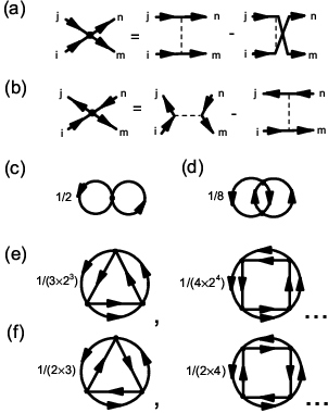
and they are diagrammatically shown in Fig. 1 (a) and (b). The Hartree-Fock (HF) and the second order $\Phi$ diagrams can be drawn easily by the bare vertices [Fig. 1 (c) and (d)]. Connecting the bare PP or PH vertices in the random-phase-approximation (RPA) series by the Green’s function $\hat{G}$, we get the main body of FLEX $\Phi$ diagrams, which is shown in Fig. 1 (e) and (f).

For the $m$-orbital system without SU(2) symmetry, the Green’s function and the self-energy can be expressed as $2m\times 2m$ matrices, satisfying the Dyson equation,

where $\hat{h}(\bm{k})$ represents the free part Hamiltonian including SOC [see Eq. (1)]. The self-energy is obtained by taking the derivative of $\Phi$ with respect to $\hat{G}$, i.e., plucking one line of Fig. 1 (c) to (f),

where the abbreviation $k\equiv[\bm{k},ik_{l}]$ ($q\equiv[\bm{q},iq_{l}]$) is used with the fermion (boson) Matsubara frequency $k_{l}=(2l+1)\pi T$ ($q_{l}=2l\pi T$). The first and second terms in Eq. (6) represent the HF and second order contributions, and the third and forth terms represent the RPA-bubbles of the PP and PH channels. The susceptibilities for these two channels are given by the $(2m)^{2}\times(2m)^{2}$ matrices,

in which the Linhard functions are defined respectively by,

Equations (5) to (8) form a closed set and thus could be solved self-consistently.

The irreducible vertex of the Bethe-Salpeter (BS) equation for the PH channel is the differentiation of self-energy (or the second derivative of $\Phi$ ) with respect to $\hat{G}$. Apparently there are two kinds of contributions: (a) the diagrams in which the plucked two lines belong to the same bubble and only single RPA-form fluctuation is included. (b) Aslamazov-Larkin (AL) diagrams in which the plucked two lines belong to different bubbles and more than one RPA-form fluctuations are taken into account. Here we omit the AL diagrams for the following reasons [17, 18, 28]: First, the AL contributions are demonstrated to be small (no more than $15\%$ for the zero-momentum static susceptibility, for example). Second, the AL contributions will aggravate the agreement between the FLEX results and the benchmark QMC simulations. Third, the AL diagrams are necessary if we require keeping the conservation law rigorously, which is believed to be essential in some transport studies[29]. Since here we investigate the equilibrium properties of electrons in the normal state, the AL diagrams can be safely removed. Therefore we obtain the PH channel’s irreducible vertex

where momenta $k$, $k^{\prime}$ are for the fermions and $Q$ is for the collective bosonic mode. The corresponding BS equation reads

where $\lambda^{h}_{Q}$ and $\hat{\psi}^{h}(k;Q)$ represent the eigenvalue and eigenfunction. Particularly, if $\lambda^{h}_{Q}$ approaches to $1$ at zero frequency, the system undergoes a spontaneously symmetry breaking at momentum $\bm{Q}$ in the PH channel.

The irreducible vertex for PP channel is the second derivative of $\Phi$ with respect to anomalous Green’s functions $\hat{F}$ and $\hat{F}^{\dagger}$ [30], here $F_{ij}=\langle T_{\tau}c_{i}c_{j}\rangle$ and $F_{ij}^{\dagger}=\langle T_{\tau}c^{\dagger}_{i}c^{\dagger}_{j}\rangle$. Although there is no anomalous Green’s function lines in the original $\Phi$ diagrams (see Fig. 1), we can construct such diagrams by replacing two $\hat{G}$ with $\hat{F}$ and $\hat{F}^{\dagger}$ but keeping two arrows pointing in and other two arrows pointing out at each dot. Here we omit the AL diagrams again and obtain the PP channel’s irreducible vertex

and the corresponding BS equation

Unlike the PH channel, the largest eigenvalue $\lambda^{p}_{Q}$ always associates with $Q=[\bm{0},0]$, indicating the formation of Cooper pairs with opposite momenta. Eqs. (11) and  (12) can be used to investigate the most favorable superconducting pairing gap which corresponds to $\hat{\psi}^{p}(k;Q)$ with the largest value of $\lambda^{p}_{Q}$.

We have completed the introduction of the formal FLEX formulations, in practical application some reasonable approximations are widely used to simplify the computations. First, when the on-site interactions are all repulsive, the contributions of the PP RPA-bubbles in Fig. 1 (e) are relatively small and therefore could be safely left out  [17, 18, 19, 31]. Second, it is more convenient to choose other numerical criterions, instead of Eq. (10), to evaluate the PH channel’s instability. For example, one can choose the Stoner-like criterion $\text{det}[\hat{1}+\hat{\Gamma}^{h}\hat{\chi}^{h0}(\bm{Q},0)]<0.002$ [19], or if the biggest element of $\chi^{h}_{ij}(\bm{Q},0)$ is 50 times larger than $\chi^{h0}_{ij}(\bm{Q},0)$ [23], as we employ in this paper.

To apply the above FLEX method to our study, the Hugenholtz vertices in Eq. (4) are fabricated by the on-site interactions ($U,U,J,J^{\prime}$), and the results presented in this paper are given by the parameters ($U,U,J,J^{\prime})=(5,3.5,0.75,0.75$), no qualitative different results are obtained when we change the values of $U$ and $J$. The numerical calculations are performed on $64\times 64$ $\bm{k}$ meshes with 1024 (for $T\!=\!0.04$), 2048 (for $T\!=\!0.02,0.015$) and 4096 (for $T\!=\!0.01$) Matsubara frequencies. Particularly, we utilize the technique developed by Deisz et al. [32] to efficiently include the contribution of high Matsubara frequencies. The analytical continuation of Green’s functions to the real frequency is carried out by Pad$\acute{\rm e}$ approximation [33]. The convergent solutions of the FLEX equations are obtained if the relative error of each matrix element of $\hat{\Sigma}$ is smaller than $10^{-6}$.

Let us first define corresponding susceptibilities for various collective excitations relevant to the following discussions. The static transverse spin (TS) and longitudinal spin (LS) susceptibilities are given by

where the spin and orbital degrees of freedom have been expressed by $(\alpha,\beta,\mu,\nu)$ and $(m,n)$, respectively. The charge fluctuation is too small compared to other fluctuations and thus is not discussed here. Because of the introduction of SOC, the contribution of orbital fluctuations is no longer neglectable, so we define the static transverse orbital (TO) and longitudinal orbital (LO) susceptibilities

As discussed in the introduction, it has been suggested that the low-energy physics in Sr₂IrO₄ may be described as an effective one-band model with the isospin $J_{\text{eff}}=1/2$[11, 12]. To check its possible application here, we define the isospin susceptibility. The creation operators for the isospin-up and isospin-down states with momentum $\bm{k}$ are given by $a^{\dagger}_{\bm{k},\Uparrow}=(d^{\dagger}_{\bm{k},1,\downarrow}+id^{\dagger}_{\bm{k},2,\downarrow}+d^{\dagger}_{\bm{k},3,\uparrow})/\sqrt{3}$ and $a^{\dagger}_{\bm{k},\Downarrow}=(d^{\dagger}_{\bm{k},1,\uparrow}-id^{\dagger}_{\bm{k},2,\uparrow}-d^{\dagger}_{\bm{k},3,\downarrow})/\sqrt{3}$, where indexes 1, 2, 3 denote $yz$, $zx$, and $xy$ orbitals. Therefore, the isospin operator can be constructed: $\bm{S}^{\alpha}_{\bm{q}}=\sum_{\bm{k}}(a^{\dagger}_{\bm{k+q},\Uparrow},a^{\dagger}_{\bm{k+q},\Downarrow})\bm{\sigma}^{\alpha}(a_{\bm{k},\Uparrow},a_{\bm{k},\Downarrow})^{\text{T}}$. Then, the static transverse isospin (TI) and longitudinal isospin (LI) susceptibilities are given by,

The static TS, LS, TO and LO susceptibilities for $3\%$ electron-doping at $T=0.01$ are shown in Fig. 2 (a)-(d). As expected, the strong peaks exist around ($\pm\pi,\pm\pi$), which are reminiscences of the AFM order in the parent compound. In particular, the intensities of orbital susceptibilities are all stronger than those of spin susceptibilities, and the TO fluctuation overwhelms the LO fluctuation. These features are consistent with the experimental results in the single-crystal neutron diffraction [4] and nonresonant magnetic X-ray diffraction [34].

Fig. 2 (e) and (f) show the TI and LI susceptibilities for the same $3\%$ electron doping at $T=0.01$. The peaks also reside at the same momenta as in the spin and orbital fluctuations. Quite strikingly, the intensity of the TI susceptibility is almost one order of magnitude larger than that of all other fluctuations. To show in more detail the effects of the isospin fluctuations, in Fig. 3 (a) we compare the maximum magnitude of $\chi^{\alpha}(\bm{q})$ at $T=0.02$, from 40% hole-doping to 30% electron-doping, with $\alpha$ denoting TI, LI, TO, LO, TS and LS channels. The AFM order is determined by the numerical criterion in the PH channel, as introduced in Sec.II B. As shown, the TI susceptibility tends to diverge as the system approaches the AFM state, from both the electron-doped side and the hole-doped side. These results suggest that the AFM order in the undoped and slightly doped system is mainly caused by the TI fluctuation. Consequently, it shows that the effective one-band model with the isospin $J_{\text{eff}}=1/2$ [11, 12] can describe the magnetic properties reasonably in the undoped and slightly doped Sr₂IrO₄. Another feature drawn from Fig. 3 (a) is that the AFM is more robust against the hole-doping in comparison to the electron-doping, which may be useful for the related experimental investigations.

When the system is doped away from the AFM region, Fig. 3 (a) shows that the TI fluctuation decreases rapidly with doping. However, it still has larger magnitude than all others in the region of 30% hole-doping to 50% electron-doping (the results for $>30\%$ electron-doping are not shown here), though their differences are decreased with dopings. In this region, the momentum $\bf q$ is at or near the $(\pi,\pi)$ point. When doping the system further with holes ($>30\%$), the spin fluctuation becomes dominant so that the effective one-band picture is broken down. These results can be understood from the weights of the $J_{\text{eff}}=1/2$ doublet and $J_{\text{eff}}=3/2$ quartet along the Fermi surface, as shown in Fig. 3 (b). One can see that the closed electron pocket centered around the $\Gamma=(0,0)$ point is composed mainly of the $J_{\text{eff}}=1/2$ doublet, while the hole pocket around $(\pi,\pi)$ mainly of the $J_{\text{eff}}=3/2$ quartet. For $40\%$ hole-doping, the hole Fermi pocket becomes large and introduces a Fermi surface nesting between the hole and electron pockets, as shown in Fig. 3 (b). Thus, the inter-pocket particle-hole scattering between the $J_{\text{eff}}=1/2$ dominant band and $J_{\text{eff}}=3/2$ dominant band takes action and overwhelms the intra-pocket scattering in the $J_{\text{eff}}=1/2$ dominant band, which makes the isospin fluctuation no longer the leading collective excitation. On the other hand, from the distribution of orbital characters shown in Fig. 3 (c), we can find that the main inter-pocket scattering occurs in the same orbital, which makes the orbital fluctuations also suppressed. Therefore, the spin fluctuation is the dominant collective excitation for the heavily hole-doped system. However, the Fermi level moves away from the $J_{\text{eff}}=3/2$ dominant band with the electron doping, consequently it is only the $J_{\text{eff}}=1/2$ dominant band that crosses the Fermi level. Therefore, the one-band picture is always robust against the electron doping. Furthermore, we have also examined the range of validity of the effective one-band picture with respect to the strength of SOC. As shown in Fig. 3 (d), the TI susceptibility prevails all others for 20% hole-doping if $\xi_{SOC}>0.8$, indicating that this picture survives in an extended range.

The pseudogap behavior can be detected from the single particle spectral function which is defined as $A(\bm{k},\omega)=-\sum_{n}\text{Im}G_{nn}(\bm{k},\omega)/\pi$, where $n$ denotes both spin and orbital indices. In Fig. 4 (a) and (b), we show the contour plot of the zero-energy spectrum at $T=0.015$ for $10\%$ and $5\%$ electron-doping, respectively. Since the system has been away from the AFM order at these dopings [see Fig. 3 (a)], an intact Fermi surface is expected in the conventional normal state. Indeed, for $10\%$ electron-doping, a closed diamond-shaped Fermi surface is observed, as shown in Fig. 4 (a). However, an obvious reduction in the spectral intensity occurs around $(0,\pi)$ and its symmetric points for $5\%$ electron-doping. This reduction is strongly temperature-dependent, because it appears only below a certain temperature, as shown in Fig. 4 (c) and (d) at $3\%$ electron-doping for $T=0.02$ and $T=0.01$, respectively. Owing to the suppression of the spectra near $(0,\pm\pi)$ and $(\pm\pi,0)$, the Fermi surface around these momenta is destructed and the four residual separated segments form the so-called Fermi arcs [see Fig. 4 (b) and (d)]. These results are consistent with the recent ARPES experiment [8]. In order to look in more detail the suppression of the spectra, we show the energy distribution curves (EDC) of the spectral functions for $3\%$ electron-doping at three momentum points near $(\pi,0)$ in Fig. 4 (e). One can see that the suppression occurs basically around the Fermi energy when the temperature is decreased from $T=0.02$ to $T=0.01$. Moreover, different from a well defined quasiparticle peak at $T=0.02$, the spectral functions at $T=0.01$ for ${\bf q}=(30\pi/32,0)$ and $(31\pi/32,0)$ show a weak dip around the Fermi energy, as shown in Fig. 4 (f). It suggests that a weak pseudogap does exist around $(\pi,0)$ and its symmetric momenta for slightly electron-doping.

Since thers is no long-range order in this doping range, the pseudogap is most likely to result from the scattering of quasiparticles by the collective excitations. In this framework, the quasiparticles around $(\pi,0)$ and $(0,\pi)$ are strongly coupled by the collective excitations with the transferred momentum $(\pi,\pi)$ in the scattering process. In accord with this analysis, the results presented in Fig. 2 demonstrate that all collective excitations, including the spin, orbital and isospin fluctuations, exhibit the characteristic momentum $(\pi,\pi)$. In particular, the transverse isospin (TI) fluctuation overwhelms the spin and orbital fluctuations. We have also carried out a careful examination, and find that all the important elements of $\hat{\chi}^{h}(\bm{q},0)$ are included in the TI fluctuation. Especially, for ${\bm{q}}=(\pi,\pi)$ the elements included in the TI susceptibility are calculated to amount to 91.3% weight of the total PH susceptibilities for 3% electron-doping at $T=0.01$. Therefore, it suggests that the scatterings of quasiprticles by the ($\pi,\pi$) TI fluctuation lead to a weak pesudogap partially opened around $(0,\pm\pi)$ and $(\pm\pi,0)$.

We have also investigated the possible pseudogap behavior and Fermi arcs in the lightly hole-doped region. The typical results of the spectral function $A(\bm{k},0)$ for 17% hole-doping are shown in Fig. 5. At $T=0.04$, there is a nearly circular Fermi surface around the $\Gamma$ point. By decreasing the temperature to $T=0.01$, the spectral weights are suppressed on some Fermi momenta and consequently it leads to the formation of the Fermi arcs. However, the suppressions now appear around $(\pi/2,\pi/2)$, which is contrary to the case of the electron-doping shown in Fig. 4 (b) and (d). This suppression also results from the ($\pi,\pi$) TI fluctuation. In this case, the Fermi surface shrinks in comparison with that of electron-doping, so that the “hot spots” (the crossing points of the Fermi surface with the boundary of the AFM Brillouin zone) at which the quasiprticles are strongly scattered move from the $(\pm\pi,0)$ and $(0,\pm\pi)$ points to the $(\pm\pi/2,\pm\pi/2)$ points (see Fig. 4 and Fig. 5).