By constructing the Riemann surface controlling the resonance structure of Winter model, we determine the limitations of perturbation theory. We then derive explicit non-perturbative results for various observables in the weak-coupling regime, in which the model has an infinite tower of long-lived resonant states. The problem of constructing proper initial wavefunctions coupled to single excitations of the model is also treated within perturbative and non-perturbative methods.

Key words: metastable state, perturbation theory, non-perturbative effect, Riemann surface, quantum mechanics, geometry.

1 Introduction

The only general analytic tool available up to now to study “realistic” quantum field theories, such as for example Quantum Chromodynamics (QCD) in four dimensions, is perturbation theory. The great variety of the electromagnetic and hadronic phenomena observed at different energies may suggest that exact solutions will be beyond human capabilities for a long time, even though there has been some recent progress in QCD in the $1/N_{c}$ expansion, with $N_{c}$ the number of colors [1]. In general, perturbative cross sections can be written schematically as:

\sigma(g)=\sum_{n=1}^{\infty}\sigma_{n}g^{n},

where the $\sigma_{n}$ ’s are real coefficients and $g$ is the coupling of the model. QCD for instance, because of asymptotic freedom, is weakly coupled in the ultraviolet, where perturbation theory is therefore a natural tool, while it is strongly coupled in the infrared. The hadron mass spectrum, the scattering lengths, the string tension, the chiral symmetry breaking scale, the parton distribution functions, the power-corrections to high-energy cross sections and event-shape distributions, etc., are all well-known examples of significant physical quantities which fall outside the reach of perturbation theory. Furthermore, being unable to exactly evaluate the $\sigma_{n}$ ’s for arbitrary $n$ , the problem of non-perturbative effects to observables is necessarily treated in a rather indirect way. In the last decades, many different approaches have been developed for this task: methods based on the summation of specific classes of diagrams (the $1/N_{c}$ expansion cited above, the renormalon calculus supplemented by the large- $\beta_{0}$ limit, etc.), toy models in lower space-time dimensions (typically two or even three), numerical Monte-Carlo computations of the euclidean theory regularized on a lattice, direct comparison of perturbative cross sections with experimental data, and so on. We may say that a large part of high-energy theoretical activity of, let’s say, the last forty years has been devoted to gain some control on the non-perturbative effects. The problem is a recurrent one in QCD and it might have been a problem also in the (standard) electroweak theory in the case of a very heavy Higgs, let’s say $m_{H}\raisebox{-3.0pt}{$\>\stackrel{{\scriptstyle<}}{{\scriptstyle\sim}}\>$}800$ GeV. In the latter case the scalar sector would become indeed strongly coupled. However, the Higgs boson was discovered at the Large Hadron Collider (LHC) in 2012 with a small mass, $m_{H}\simeq 125$ GeV, as previously indicated by indirect measurements, so the problem of non-perturbative electroweak effects has at present a limited phenomenological relevance. In general, by using a (truncated) perturbative computation of a quantum field theory model to describe some specific phenomenology ranging, let’s say, from high- $T_{c}$ superconductivity to strong interactions, one is always faced with the problem of ”what is missing”, i.e. which effects lie in the unevaluated terms or are actually ”invisible” to perturbation methods. In such a situation, it may be interesting to study a model which, though not a quantum field, can be analyzed both in perturbative and non-perturbative way. It is in this spirit that we present a systematic study of the so-called Winter model [2, 3, 4, 5, 6], a non-relativistic quantum mechanics model possessing, in the weak-coupling regime, an infinite tower of resonant states coupled to a continuum [7], with Hamiltonian in proper units:

\hat{H}=-\frac{\partial^{2}}{\partial x^{2}}+\frac{1}{\pi g}\delta(x-\pi)

(1)

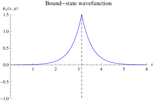
on the half line $x\geq 0$ with vanishing boundary conditions in the origin, $\psi(x=0,t)=0$ . $g\in{\mathbb{R}}$ is the only coupling of the model. Winter’s model has an unstable energy spectrum in the free limit $g\to 0$ : for $g\to 0^{+}$ the spectrum is uniformly bounded from below by zero, while for $g\to 0^{-}$ the spectrum is unbounded because of the appearance of an eigenfunction in the discrete spectrum with energy $\varepsilon(g)\simeq-1/(4\pi^{2}g^{2})\to-\infty$ (see fig.1). The free limit is therefore a singular one. In classical terms, the particle falls in the potential trap located at $x=\pi$ .

Refer to caption — Figure 1: Energy spectrum of the Winter model (arbitrary units). Repulsive case ( $g>0$ ) on the left of the vertical line (in red); attractive case ( $g<0$ ) on the right (in blue). Note the discrete line in the latter case.

The instability is related to the behavior just of the fundamental state (i.e. of the state with the lowest energy) for $g\to 0$ , i.e. to the non-trivial “vacuum structure” in a small neighborhood of the free theory (see fig.2).

Furthermore, transition amplitudes for $-1<g<0$ contain contributions of the form $e^{1/g}$ , coming from the bound state, non-analytic in the origin, which are typical of non-perturbative quantum field theory effects. A similar instability in Quantum Electrodynamics (QED) was conjectured in the 50’s by F. Dyson [8] ¹¹ 1 An instability mechanism similar to the QED one also occurs in the scalar $\lambda\varphi^{4}$ theory, as well as in the simple case of a (quantum) anharmonic oscillator [9]. . For $0<\alpha\ll 1$ , where $\alpha\equiv e^{2}/(4\pi)$ is the fine structure constant of QED²² 2 Experimentally $\alpha\cong 1/137$ at low energies. with $e$ the electron charge, the fundamental state is the vacuum, i.e. the ”empty” state, without any electron-positron pair or any photon. Because of field fluctuations, electron-positron pairs (as well as photons) come out of the vacuum as virtual particles only, as their creation as real particles would increase the energy. On the other hand, for $\alpha<0$ particles with equal charges attract each other, while electrons and positrons repel each other, so that the Coulomb energy associated with an $e^{+}e^{-}$ pair is positive. The rest energy of a system containing $N$ pairs is $2Nmc^{2}$ , with $m$ the electron mass — proportional to $N$ — while the potential energy is of order $|\alpha|N^{2}/\lambda_{c}$ — proportional to $N^{2}$ — where $\lambda_{C}\equiv\hbar/(m_{e}c)$ is the electron Compton wavelength. That implies that the potential energy overcomes the rest energy for large enough $N$ . As a consequence, a huge quantity of $e^{+}e^{-}$ pairs can be created as real particles out of the vacuum, which would then decay into a state full of electrons and positrons, by lowering its energy to arbitrarily negative values. The physical picture is the following: the $e^{+}e^{-}$ pairs are created close to each other, let’s say within their Compton wavelength (the $QED$ interaction is local) and then, to minimize the energy, all the electrons fly on one side, coming close to each other, with the positrons flying on the opposite side. This spontaneous polarization of the vacuum should also occur in the usual particle states of the Fock space³³ 3 The above argument is qualitative and does not provide any estimate of the decay time.. This instability of $QED$ in a neighborhood of $\alpha=0$ was related by Dyson to the divergence of the perturbative series in $\alpha$ . The spectrum instability of Winter model in a neighborhood of the free theory might suggest that also its perturbative expansion around $g=0$ is divergent — perhaps asymptotic to the exact theory for $g\to 0$ , as is supposed to be in QED. The reality is actually more intricate; after all, physical intuition is based on $g\in{\mathbb{R}}$ , while a full understanding of the model, as we are going to show in detail, requires to complexify $g$ . It turns out that the resonances of the model, which behave in space-time for $x>\pi$ (i.e. outside the cavity) as

e^{\,ikx\,-\,ik^{2}t}

(2)

with $k\in{\mathbb{C}}$ , are controlled by a multivalued function

w\,=\,h(z)

(3)

which is the inverse of the entire function

z\,=\,\frac{e^{w}-1}{w},

(4)

where $w\equiv 2\pi ik$ and $z\equiv-g$ .⁴⁴ 4 The minus sign in front of $g$ is inserted just for practical convenience. The transcendental (infinite order) multivaluedness of $h$ is related to the fact that the model has an infinite tower of resonances. Each resonance, let’s say the $n$ -th one with $n$ a non-zero integer, is associated to a sheet $S_{n}$ of the Riemann surface $S$ of $h$ ; there is also an additional sheet, $S_{0}$ , related to the bound state. Each $S_{n}$ , with $n\neq 0$ , has order-one (square-root) branch points in

c_{n}\,\approx\,\frac{i}{2\pi n}

(5)

and at infinity, connecting $S_{n}$ to $S_{0}$ . That implies that $S_{0}$ has a countable set of order-one branch points $\{c_{n}\}_{n\neq 0}$ accumulating at the origin as

c_{n}\to 0\,\,\,\,\,\,\,\,\,\,{\rm for}\,\,\,\,\,n\to\pm\infty.

(6)

It also follows that different sheets, $S_{n}$ and $S_{k}$ with $n,k\neq 0$ , ”talk to each other” only indirectly, through $S_{0}$ , which is a different (and more complicated) sheet with respect to all the other ones. Let us also observe that the square-root branch point is, in some sense, the most general coupling between different sheets one could think of. The perturbative expansions (series in powers of $g$ ) of quantities related to the $n$ -th resonance (wave-vector, frequency, width, etc.) are convergent within a disk centered in $g=0$ of radius

R_{n}\,=\,\left|c_{n}\right|\approx\,\frac{1}{2\pi n}.

(7)

The convergence radius is then controlled by the branch point $c_{n}$ connecting $S_{n}$ to $S_{0}$ . A non-zero radius of convergence for the expansion around zero was expected on physical ground but, remaining in the physical domain $g\in{\mathbb{R}}$ , one could not have derived in a natural way its value. The instability of the spectrum, discussed above on physical ground, manifests itself mathematically in the fact that, according to eq.(6), the origin of the “bound-state sheet” $S_{0}$ is a non-isolated singularity. The above property is related to the specific geometric structure of $S$ : if the square-root branch points had coupled, for example, $S_{n}$ to $S_{n+1}$ for any integer $n$ , the point $g=0$ would have been instead an analyticity point for $S_{0}$ . For quantities related to the bound state (such as its energy, its wavefunction, etc.) no convergent power-series expansion around $g=0$ exists. While in the case of $QED$ the instability of the vacuum is expected to manifest also in any state of the Fock space, in the Winter model it is restricted to the fundamental state. The second implication of eq.(6) is that

R_{n}\to 0\,\,\,\,\,\,\,\,\,{\rm for}\,\,\,\,\,n\to\pm\infty.

(8)

The consequence is that perturbation theory can accurately describe the dynamical properties involving a finite number of resonances for small enough coupling, but it cannot describe quantities involving an infinite number of them. We will see that also the second class of observables contains fundamental physical quantities.

Our motivation to further investigate Winter model might suggest that it is just a toy model for quantum field theory: that is not actually the case [10]. Since it describes particles confined by potential barriers, with tunable efficiency, it is still currently used in quantum chemistry, together with its natural generalizations [11, 12, 13]. Let’s schematically summarize the history of Winter model relevant to the present work. As far as we know, this model was originally introduced in [2], where the resonance properties of the spectrum for a small positive coupling were analyzed. The temporal evolution of metastable states of sinusoidal shape concentrated at $t=0$ inside the cavity — the segment $[0,\pi]$ — was studied in [3]. In this work, post-exponential power corrections in time were explicitly calculated, confirming a previous general analyticity argument about the breakdown of the exponential behavior at very large times. In ref.[5] Winter’s computation was repeated, finding additional ”non-diagonal” contributions to the exponential time evolution, which had been overlooked in [3]. These new terms imply a coupling of the initial state with all the resonances of the model and not just with a single one. The off-diagonal terms a small coupling $\mathcal{O}(g)$ compared to the one in [3], but decay in general slower in time, dominating then the wavefunction in a large temporal region. Actually, most of the non-trivial properties of Winter model — resonance mixing in particular — are consequences of this additional contributions to time evolution recently discovered. In [5] it was also found that the coupling of the initial state to the resonances was controlled at first order in $g$ by an infinite matrix of the form

U(g)=1+gA,

(9)

with $A$ a real antisymmetric matrix (see eq.(132)). $U(g)$ is then an infinitesimal rotation in the infinite-dimensional vector space of the resonances. It was then natural to conjecture that higher-orders in $g$ would have led to the exponentiated form, i.e. to the unitary matrix

U(g)=\exp(gA)=1+gA+\frac{g^{2}}{2}A^{2}+\cdots.

(10)

In order to check this structure, the second-order computation in $g$ of $U(g)$ was made in [6]. In addition to the expected term $g^{2}A^{2}/2$ , it was also found a ”large” term not compatible with any generalized form of exponentiation, whose physical interpretation was problematic. A possible investigation at that point could have been to push the perturbative expansion to $\mathcal{O}(g^{3})$ , in order to have some hint of the general structure and eventually resum the expansion at all orders in $g$ , in the spirit of classical quantum-field-theory investigations. In this work however we follow a different route: we abandon perturbation theory and perform an analytic study in the complex plane of the functions controlling the expansion above for $U(g)$ . As we are going to show, that allows us to determine the convergence region of the perturbative expansion and to find explicit non-perturbative formulas for relevant observables which replace the perturbative ones outside their convergence region.

This work is at the border of different areas: 1) quantum field theory, in particular high-energy theoretical physics, where the interplay between perturbative and non-perturbative effects is crucial, as already discussed; 2) mathematical physics, as we investigate the analytic and geometric structure of the Winter model and finally 3) quantum physics —quantum chemistry in particular — where generalized Winter models are currently investigated. Therefore, since the paper is of potential interest to readers with different backgrounds, we tried to be as simple and explicit as we could. The paper is organized as follows. In sec.2 we summarize the properties of the spectrum of the Winter model and we discuss in particular the free limit $g\to 0$ , in which the system decomposes in two non-interacting subsystems, a particle in the box $[0,\pi]$ and a particle in the half-line $[\pi,\infty)$ . All that is in complete agreement with physical intuition. In sec.3 we schematically discuss the time evolution of wavefunctions initially concentrated inside the cavity and of sinusoidal shape. We also treat, in general terms, perhaps the most significant effect in the evolution of metastable states of Winter model: the above mentioned mixing of the resonances. In sec.4 we specify the discussion on resonance mixing by using explicit power expansions in $g$ and we discuss the problems associated with the perturbative expansion. In sec.5 we abandon perturbation theory and investigate the structure of the Riemann surface $S$ of the multivalued function $w=h(z)$ controlling the behavior of the resonances and the form of the infinite mixing matrix $U(g)$ . In sec.6 we re-analyze the properties of the resonances and of the mixing matrix by means of the exact (non-perturbative) information obtained with the previous geometric study. We deal again, in particular, with the problems encountered with perturbation methods. Finally, in sec.7 we draw our conclusions and we discuss some natural developments of our work. There are also three appendices. In appendix A we discuss the connection of our function $h$ with the Lambert $W$ function [14], a kind of generalization of the complex logarithm. In appendix B we present a general treatment, as well as explicit formulas, for the branch points of the function $h$ , which are crucial in our analysis. Finally, in appendix C we show that the expansion for large $|z|$ of $h(z)$ , which involves the composition of the complex logarithm with itself, actually has exactly the same multivaluedness as $h$ , which is just logarithmic. to

2 Winter Model

In general, the Hamiltonian operator of the Winter model reads:

\hat{H}\,=\,-\,\frac{\hbar^{2}}{2m}\frac{\partial^{2}}{\partial x^{2}}\,+\,\lambda\,\delta(x-L)\,,

(11)

where $m$ is the mass of the particle, $\lambda$ is a (real) coupling constant and $\delta(x-L)$ is the Dirac $\delta$ -function with support in $x=L>0$ [15]. The domain is the half-line $0\leq x<\infty$ and we assume vanishing boundary conditions at zero:⁵⁵ 5 Equivalently, one may think to the problem in the whole real axis, $x\in{\mathbb{R}}$ , with an additional infinite potential for $x<0$ .

\psi(x=0,t)=0,\,\,\,\,\,\,\,\,\,t\in{\mathbb{R}}.

(12)

Formulas can be simplified by going to a proper adimensional coordinate via

x=\frac{L}{\pi}x^{\prime}

(13)

and rescaling the Hamiltonian as:

\hat{H}=\frac{\hbar^{2}\pi^{2}}{2mL^{2}}\hat{H}^{\prime}.

(14)

The new (adimensional) Hamiltonian then takes the form in which it appears in the introduction:

\hat{H^{\prime}}\,=\,-\,\frac{\partial^{2}}{\partial x^{\prime\,2}}\,+\,\frac{1}{\pi g}\,\delta(x^{\prime}-\pi),

(15)

and contains the single (real) parameter

g\,=\,\frac{\hbar^{2}}{2m\lambda L}.

(16)

The time-dependent Schrodinger equation

i\hbar\frac{\partial\psi}{\partial t}=\hat{H}\psi

(17)

now reads

i\frac{\partial\psi}{\partial t^{\prime}}=\hat{H^{\prime}}\psi,

(18)

where time is rescaled as

t^{\prime}\equiv\frac{\hbar\pi^{2}}{2mL^{2}}t.

(19)

Let us omit primes from now on for simplicity’s sake. It is possible to rescale the Winter Hamiltonian (11) in different ways, as made for example by Winter itself in [3]. The main point however is that we deal in any case with a one-parameter model describing the coupling of a cavity (the segment $0\leq x\leq\pi$ ) with the outside (the half-line $x\geq\pi$ ). As we are going explicitly to show in the next sections and as anticipated in the introduction, for $|g|\ll 1$ resonant long-lived states inside the cavity come into play.

2.1 Spectrum

For $g>0$ there is only a continuous spectrum, with eigenfunctions of the form [2, 3, 5] (see figs.3 and 4)

	$\displaystyle\psi(x;\,k,g)$	$\displaystyle=$	$\displaystyle\sqrt{\frac{2}{\pi}}\frac{1}{\sqrt{4a(k,g)b(k,g)}}\Big\{\theta(\pi-x)\,\sin(kx)\,+\,$		(20)
			$\displaystyle\,\,\,\,\,\,\,\,\,\,\,\,\,\,\,\,\,\,\,\,\,\,\,\,\,+\,\theta(x-\pi)\big[a(k,g)\,e^{ikx}\,+\,b(k,g)\,e^{-ikx}\big]\Big\}\,$		(20)

and energies

\varepsilon(k)=k^{2}>0.

(21)

The function $\theta(y)=1$ for $y>0$ and zero otherwise is the Heaviside step function and the square root in eq.(20) is the arithmetical one, as $a(k,g)b(k,g)>0$ for any $k,g\in{\mathbb{R}}$ (an over-all phase is in any case irrelevant). The coefficients entering the eigenfunctions have the following explicit expressions:

	$\displaystyle a(k,g)$	$\displaystyle=$	$\displaystyle-\,\frac{i}{2}\,+\,\frac{1}{4\pi gk}\left[\exp(-2\pi ik)-1\right]\,;$		(22)
	$\displaystyle b(k,g)$	$\displaystyle=$	$\displaystyle+\,\frac{i}{2}\,+\,\frac{1}{4\pi gk}\left[\exp(+2\pi ik)-1\right]\,.$		(23)

These coefficients have the following two symmetries:

a(-k,g)\,=\,-b(k,g);\,\,\,\,\,\,\,\,\,\,\,\,\overline{a(k,g)}\,=\,b\left(\overline{k},\overline{g}\right),

(24)

where the bar denotes complex conjugation. The first equation says that $\psi(x;\,k,g)$ is an odd function of $k$ and implies that the zeroes of $a$ are opposite to those ones of $b$ , i.e. that if

b\left(k_{0},g\right)\,=\,0,

(25)

then

a\left(-k_{0},g\right)\,=\,0.

(26)

The second equation implies that the zeroes of $a$ are the complex conjugates of the zeroes of $b$ for conjugate coupling, i.e. that if

b\big(k_{0},g\big)\,=\,0,

(27)

then

a\left(\overline{k_{0}},\overline{g}\right)\,=\,0\,.

(28)

For real $g$ , the zeroes of $a$ are then the complex conjugates of the zeroes of $b$ . From the two properties above it is possible to reconstruct for real $g$ all the zeroes of $a$ and of $b$ , for example, from the zeroes of $b$ in the forth quadrant. Finally, note that for real $k$ and $g$

\overline{a(k,g)}\,=\,b\left(k,g\right),\,\,\,\,\,\,\,\,\,\,\,\,k,\,g\in{\mathbb{R}},

(29)

so that

a(k,g)b(k,g)\,=\,|a(k,g)|^{2}\,=\,|b(k,g)|^{2},\,\,\,\,\,\,\,\,\,\,\,\,k,\,g\in{\mathbb{R}}.

(30)

In eq.(20) we have assumed the standard continuum normalization:

\int_{0}^{\infty}\overline{\psi(x;\,k^{\prime},g)}\,\psi(x;\,k,g)\,dx\,=\,\delta(k-k^{\prime})\,,

(31)

with $\delta(q)$ the Dirac $\delta$ -function. The quantity $k$ is a real quantum number but, since the eigenfunctions are odd functions of $k$ , one can assume $k>0$ ⁶⁶ 6 The case $k=0$ has to be discarded as one obtains in this case, because of the boundary condition, the zero function, which is not an acceptable wavefunction.. Note that the spectrum is bounded from below by zero, uniformly in $g>0$ . As we are going to show in the next section and as anticipated in the introduction, that is no more the case for $g<0$ , because of the appearance of a discrete spectrum. The eigenfunctions can also be written in trigonometric form as [2]:

\psi(x;k,g)\,=\,\sqrt{\frac{2}{\pi}}\,\Big\{\theta(\pi-x)\,A(k,g)\sin\big[k\,x\big]+\theta(x-\pi)\,\sin\big[k\,x+\varphi(k,g)\big]\Big\}.

(32)

The inside amplitude is given by (see fig.(5))

A(k,g)=\frac{1}{2\sqrt{a(k,g)b(k,g)}}=\frac{1}{\sqrt{1\,+\,1/(\pi gk)\sin 2k\pi\,+\,1/(2\pi^{2}g^{2}k^{2})(1-\cos 2k\pi)}}.

(33)

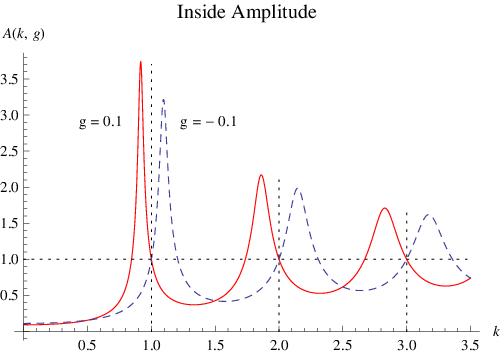
Note that⁷⁷ 7 It may be argued that $A(k,g)$ , as a function of $k$ , resembles the shape of the total cross section of electron-positron annihilation into hadrons as a function of the c.o.m. energy $\sqrt{s}$ , $\sigma(e^{+}e^{-}\to h^{\prime}s)$ , above a heavy quark-antiquark pair threshold. Roughly speaking, the quarkonium states correspond to the resonances of the particle inside the cavity.

\lim_{k\to\infty}A(k,g)=1,

(34)

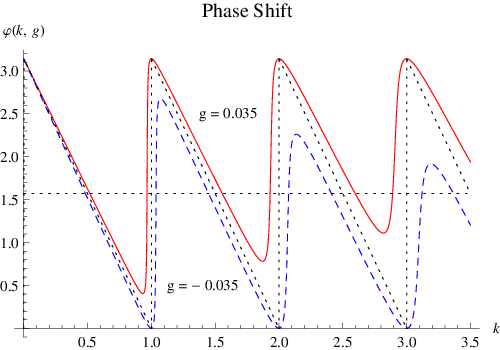
as expected on physical ground: high-energy states do not see the barrier. The phase shift between the outside amplitude and the inside one reads (see fig.6):

\cot\big[\varphi(k,g)\big]\,=\,-\frac{\pi gk}{\sin^{2}(\pi k)}-\cot(\pi k).

(35)

For the cotangent to be invertible, let us assume for its argument the following range:

-\pi<\varphi(k,g)<0\,\,\,\,\,\,\,\,\mathrm{for}\,\,\,\,\,g>0;\,\,\,\,\,\,\,\,\,\,\,\,\,\,\,\,\,\,\,\,0<\varphi(k,g)<\pi\,\,\,\,\,\,\,\,\mathrm{for}\,\,\,\,\,g<0.

(36)

With the above choice of the argument,

\lim_{k\to+\infty}\varphi(k,g)=0,

(37)

i.e. there is no phase shift in the high-energy limit, in agreement with physical intuition.

2.2 Strong-Coupling Regime

Even though we are mostly interested to the weak-coupling regime $|g|\ll 1$ — to be more specific, to subtle weak-coupling properties — let us briefly consider the strong coupling regime

|g|\gg 1.

(38)

Waves find in this case a small barrier at the point $x=\pi$ ; in the strong coupling limit $g\to\pm\infty$ , the Dirac potential completely disappears and the Winter Hamiltonian becomes then the Hamiltonian of a free particle,

\hat{H}_{0}=-\frac{\partial^{2}}{\partial x^{2}},

(39)

on the positive axis, $x\geq 0$ , with vanishing boundary conditions at the origin. Note also that

A(k,g)\to 1\,\,\,\,\,\mathrm{and}\,\,\,\,\,\varphi(k,g)\to 0\,\,\,\,\,\,\,\,\,\,\,\,\,\,{\rm for}\,\,\,\,\,\,\,g\to\pm\infty.

(40)

A duality therefore exists between the strong-coupling regime of the Winter model $|g|\gg 1$ and the weak-coupling regime of a particle on the positive axis subjected to a small potential. Let us remark that there is continuity in going from the strong coupling regime, $|g|\gg 1$ , to the weak-coupling one, $|g|\ll 1$ . As we are going to show in the next section, the only singular limit is $g\to 0$ .

2.3 Weak-Coupling Regime and Free Limit

We are interested to the weak-coupling regime $0<g\ll 1$ and to the free limit of the model $g\to 0^{+}$ [5]. It is clear that, unlike the previous case, taking this limit directly in the Hamiltonian, which has a pole in $g=0$ , is meaningless⁸⁸ 8 This is to be compared with quantum field theory, in which the coupling to be sent to zero usually appears in the numerator. The $QED$ Lagrangian density, for example, reads $\mathcal{L}=-\frac{1}{4}F_{\mu\nu}F^{\mu\nu}+\bar{\psi}\left(i\gamma_{\mu}\partial^{\mu}-m\right)\psi+e\bar{\psi}\gamma_{\mu}\psi A^{\mu},$ (41) where $F_{\mu\nu}$ is the field tensor and $A^{\mu}$ the gauge potential of the electromagnetic field, $\psi$ is the Dirac field, $e$ the electron charge, and the free limit is $e\to 0$ . . We therefore take the free limit on the eigenfunctions (which is instead meaningful) and then find which Hamiltonian has the limiting eigenfunctions.

For $k$ not close to an integer within $\mathcal{O}(g)$ , namely

k\neq n+\mathcal{O}(g),

(42)

with $n$ a non-zero integer,

|a(k,g)|\,=\,|b(k,g)|\,=\,\mathcal{O}\left(\frac{1}{g}\right),

(43)

implying that the eigenfunctions have a small amplitude $\mathcal{O}\left(g\right)\ll 1$ inside the cavity — outside the cavity the amplitude is always $\mathcal{O}(1)$ , no matter which values are chosen for $k$ and $g$ , because of continuum normalization. With the generic values of $k$ given by eq.(42), outside waves are not able to excite appreciably the cavity. In the limit $g\to 0^{+}$ the eigenfunctions exactly vanish inside the cavity.

Let us then consider the phase behavior of the eigenfunctions. Unlike the discussion on the amplitude, let us first consider the free case. For $g=0$ , one obtains:

\varphi=\varphi_{s}(k,\,g=0)=-\pi k+s\pi,

(44)

where $s$ is any integer. The eigenfunctions therefore read:

\psi(x;\,k,\,g=0)\,=\,(-1)^{s}\theta(x-\pi)\sqrt{\frac{2}{\pi}}\sin\big[k(x-\pi)\big],\,\,\,\,\,\,\,\,\,\,\,\,\,\,k>0,\,\,\,\,\,k\,\neq\,n+\mathcal{O}(g),

(45)

with $n$ a positive integer. In order to satisfy eq.(36), the integer $s$ has to be a function of $k$ but, since an overall phase is not observable, one can take once and for all for example $s=0$ , obtaining the usual eigenfunctions of a particle confined to the half-line $x\geq\pi$ , with vanishing boundary conditions,

\psi(x=\pi;\,k,\,g=0)\,=\,0.

(46)

The phase $\varphi(k,g)$ does not provide any measurable information in the free case: it does not transfer any information from inside the cavity to outside it. In other words, the cavity is impermeable also as far as the phase $\varphi$ is concerned. Let us now consider the interacting case, $0<g\ll 1$ . For the non-exceptional values of $k$ in eq.(42), it holds

\sin(\pi k)=\mathcal{O}(1)

(47)

and the additional term in $\varphi(k,g)$ due to the interaction is just a small correction with respect to the free case:

\frac{\pi gk}{\sin^{2}(\pi k)}\,=\,\mathcal{O}(g).

(48)

Therefore there is not any qualitative change of the profile of $\varphi(k;g)$ in the region of generic $k$ ’s given by eq.(42) (see fig.6).

Let us now see what happens for $0<g\ll 1$ and for $g\to 0^{+}$ to the amplitudes and phases of the eigenfunctions for the complementary values of $k$ , i.e. for the “exceptional” values

k\,\simeq\,n-ng,

(49)

with $n$ any non-zero integer. Since

\left|a\big[n(1-g),g\big]\right|\,=\,\left|b\big[n(1-g),g\big]\right|\,=\,\frac{\sqrt{1+\pi^{2}n^{2}}}{2}\,|g|\,+\,\mathcal{O}\left(g^{2}\right),

(50)

the amplitude of $\psi(x;k,g)$ inside the cavity shows marked peaks. In the limit $g\to 0^{+}$

\left|a\big[n(1-g),g\big]\right|\,=\,\left|b\big[n(1-g),g\big]\right|\,\to\,0

(51)

and the inside amplitude diverges. This divergence, which (at face value) is physically meaningless, actually signals a qualitative change of the spectrum. To have a finite amplitude inside the cavity for $g\to 0$ , one has to impose that the eigenfunctions exactly vanish outside it, necessarily obtaining states with a finite normalization. Therefore a discrete spectrum emerges out of the continuum one for the exceptional $k$ -values in eq.(49) when

g\to 0\,\,\,\,\,\,\,\,\,\,\,\,{\rm so}\,\,\,{\rm that}\,\,\,\,\,\,\,\,\,k\simeq n(1-g)\to n.

(52)

By normalizing these eigenfunctions to one, we obtain:

\sqrt{\frac{2}{\pi}}\,\theta(\pi-x)\,\sin(nx),

(53)

with $n$ a positive integer. The above ones are the eigenfunctions of a particle confined to the segment $0\leq x\leq\pi$ .

As far as the phase behavior is concerned, the term on the l.h.s. of eq.(48) has a double pole for $k\to\,\mathrm{integer}$ , while the $g$ -independent term in eq.(35), $\cot(\pi k)$ , only has a simple pole. The consequence is that the term proportional to $g$ is not uniformly small in $k$ even for $|g|\ll 1$ and actually dominates for $k\to$ integer. In the region specified by eq.(49)

\varphi\,\simeq\,\mp\frac{\pi}{2}

(54)

for $g>0$ and $g<0$ respectively. Furthermore, $\varphi(k,g)$ passes through $\mp\pi/2$ with a high slope when $k$ passes through $n(1-g)$ :

\left.\frac{\partial\varphi}{\partial k}\right|_{k=n(1-g)}=\frac{\pi}{1+\pi^{2}n^{2}}\,\frac{1}{g^{2}}+\mathcal{O}\left(\frac{1}{g}\right).

(55)

This sudden phase variation is a typical resonant behavior [16]. An important point is that, unlike the free case, $\varphi(k;g\neq 0)$ is a continuous function of $k$ and is a measurable. In the limit $g\to 0$ the phase $\varphi(k,g)$ develops infinite slopes at the integers $k=n$ (see fig.6).

By looking at eqs.(49), (50) and (55), one may observe that the “effective coupling” of the $n$ -th resonance to the continuum rather than $g$ is actually $\approx ng$ . That implies that one has to face strong-coupling phenomena for large $n$ even when $|g|\ll 1$ , because the perturbative expansion involves powers of $ng$ rather than powers of $g$ : we will make these considerations more precise in later sections.

We can summarize the above findings by saying that, in the free limit, the system described by the Winter Hamiltonian decomposes into two non-interacting subsystems. The first subsystem is particle in a box, with Hamiltonian

\hat{H}_{1}=-\frac{\partial^{2}}{\partial x_{1}^{2}},\,\,\,\,\,\,\,\,\,\,\,\,\,\,\,0\leq x_{1}\leq\pi,

(56)

with vanishing boundary conditions:

\psi_{1}(x_{1}=0,\,t)=\psi_{1}(x_{1}=\pi,\,t)=0,\,\,\,\,\,\,\,\,\,\,\,t\in{\mathbb{R}}.

(57)

As well known, this system has an infinite tower of discrete states,

\psi_{1}^{(n)}(x_{1})=\sqrt{\frac{2}{\pi}}\sin\left(nx_{1}\right),

(58)

with $n\in{\mathbb{N}}_{+}$ , and no continuum spectrum. The second subsystem is a particle in a half-line, with Hamiltonian

\hat{H}_{2}=-\frac{\partial^{2}}{\partial x_{2}^{2}},\,\,\,\,\,\,\,\,\,\,\,\,\pi\leq x_{2}<\infty,

(59)

with wavefunctions vanishing at the only boundary point $x=\pi$ :

\psi_{2}(x_{2}=\pi,\,t)=0,\,\,\,\,\,\,\,\,\,t\in{\mathbb{R}}.

(60)

$\hat{H}_{2}$ has a continuous spectrum only, with eigenfunctions (normalized to a $\delta$ -function) of the form

\psi_{2}\left(x_{2};k\right)=\sqrt{\frac{2}{\pi}}\sin\left[k(x_{2}-\pi)\right],

(61)

with $k>0$ . Therefore Winter Hamiltonian $\hat{H}(g)$ factorizes in the limit $g\to 0^{+}$ in the sum of the Hamiltonian of a particle in a box and the Hamiltonian of particle in a half-line:

\lim_{g\to 0^{+}}\hat{H}(g)=\hat{H}_{1}+\hat{H}_{2}.

(62)

2.4 Resonances

To study the decay, as well as the formation, of metastable states, it is convenient to introduce generalized eigenfunctions $\psi(x;\,k,g)$ with $k\in{\mathbb{C}}$ , called resonances or antiresonances, which satisfy purely outgoing or purely incoming boundary conditions, i.e.

\left(\frac{d}{dx}-ik\right)\psi(x;\,k,g)=0\,\,\,\,\,\,\,\,\,\,\mathrm{for}\,\,\,\,\,x>\pi,

(63)

with

\mathrm{Re}\,k>0\,\,\,\,\,\mathrm{or}\,\,\,\,\,\mathrm{Re}\,k<0

(64)

respectively. Let us remark that while in the case of the Winter model the boundary condition above, implying

\psi(x;\,k,g)\,\approx\,e^{ikx},

(65)

can be imposed at any point outside the cavity, for a general short-range potential, one has to impose it at $x\to+\infty$ . By equating to zero the coefficient $b(k,g)$ of the component $\exp(-ikx)$ in $\psi(x;\,k,g)$ (see eq.(20)), we obtain the transcendental equation in $k$

\exp(2\pi ik)\,+\,g2\pi ik\,-1\,=\,0,

(66)

having a countable set of solutions $\{k^{(n)}(g)\}$ lying in the lower half of the $k$ -plane,

\mathrm{Im}\,k^{(n)}(g)\,<\,0

(67)

and reading for $|g|\ll 1$ :

k^{(n)}(g)\,=\,n(1-g+g^{2})-i\pi n^{2}g^{2}+\mathcal{O}\left(g^{3}\right),

(68)

where $n$ is any non-zero integer. For $n>0$ , the zeroes lie in the forth quadrant and are associated to resonances, while for $n<0$ they lie in the third quadrant and are associated to antiresonances. In general, the functions $k^{(n)}(g)$ ’s with $n\neq 0$ are defined as the zeroes of the transcendental equation above,

b\left[k^{(n)}(g),g\right]\equiv 0,

(69)

satisfying the initial condition

k^{(n)}(g=0)\,=\,n.

(70)

These functions are fundamental elements of the Winter model. In the next section we will present a higher-order perturbative expansion for $k^{(n)}(g)$ — as already noted, we will find that the expansion parameter, rather than $g$ , is actually $gn$ . In sec.(5), in order to fully understand their properties, we will analytically continue the $k^{(n)}(g)$ ’s for complex $g$ . All the $k^{(n)}(g)$ ’s will turn out to be the various branches of the multivalued function $k=k(g)$ implicitly defined by $b\left[k(g),g\right]\equiv 0$ .

Because of the first symmetry between the functions $a(k;g)$ and $b(k;g)$ discussed in the previous section, the zeroes $\{\chi^{(n)}(g)\}$ of the function $a(k;g)$ have a positive imaginary part for any $n\neq 0$ . They can be defined as

\chi^{(n)}(g)\,\equiv\,-k^{(n)}(g)\,=\,-n(1-g+g^{2})+i\pi n^{2}g^{2}+\cdots

(71)

and are associated to resonances for $n>0$ (second quadrant) and to antiresonances for $n<0$ (first quadrant). Roughly speaking, because of the first symmetry between the coefficients, all the dynamical information is already contained in just one coefficient; we have therefore considered explicitly only the coefficient $b(k;\,g)$ . By using also the second symmetry, one can easily show that for $g\in{\mathbb{R}}$ the real part of $k^{(n)}(g)$ is odd in $n$ , while the imaginary part is even in $n$ . From the relation

\chi^{(n)}(g)\,=\,\overline{k^{(-n)}(g)}

(72)

it follows indeed

k_{1}^{(n)}(g)+ik_{2}^{(n)}(g)\,=\,-k_{1}^{(-n)}(g)+ik_{2}^{(-n)}(g),

(73)

where $k^{(n)}(g)=k_{1}^{(n)}(g)+ik_{2}^{(n)}(g)$ with $k_{1}^{(n)}(g),\,k_{2}^{(n)}(g)\in{\mathbb{R}}$ . For real $g$ the Winter Hamiltonian is real and therefore time-reversal invariant, so that the formation and the decay of a resonance occur in the same way.

According to the formula above, for $n=0$ one would obtain $k^{(0)}(g)\equiv 0$ ; unlike the other cases, the function $k^{(0)}(g)$ does not posses a convergent expansion in powers of $g$ . Relevant expansions in this case are an expansion in powers of $g+1$ for $|g+1|\ll 1$

k^{(0)}(g)\,\simeq\,\frac{i}{\pi}(g+1)\,+\,\frac{2i}{3\pi}(g+1)^{2}\,+\,\mathcal{O}\left[(g+1)^{3}\right]\,,

(74)

as well as an expansion involving exponentials and poles for $g<0$ , $|g|\ll 1$ :

k^{(0)}(g)\,=\,-\,\frac{i}{2\pi g}\Big[1-e^{1/g}+\mathcal{O}\left(e^{2/g}\right)\Big]\,.

(75)

We will see the physical significance of these expansions in the next section. Let us remark that $k^{(0)}(g)$ is a purely imaginary number for $g\in{\mathbb{R}}^{-}$ , with a positive imaginary part for

-1<g<0.

(76)

The latter case corresponds to an exponentially decaying wavefunction for $x\to+\infty$ with negative energy, i.e. a bound state.

Coming back to the resonances, we obtain for their wavefunctions ( $n>0$ ):

	$\displaystyle\theta^{(n)}(x,t;g)$	$\displaystyle\equiv$	$\displaystyle\sqrt{\frac{2}{\pi}}\left\{\theta(\pi-x)\,\sin\left[k^{(n)}(g)x\right]+\theta(x-\pi)\,\frac{\pi gk^{(n)}(g)}{2\pi igk^{(n)}(g)-1}\,e^{i\,k^{(n)}(g)\,x}\right\}\times$		(77)
			$\displaystyle\,\,\,\,\,\,\,\,\,\,\,\,\,\,\,\,\,\,\,\,\,\,\,\,\,\,\,\,\,\,\,\,\,\,\,\,\,\,\,\,\,\,\,\,\,\,\,\,\,\,\,\,\,\,\,\,\,\,\,\,\,\,\,\,\,\,\,\,\,\,\,\,\,\,\,\,\,\,\,\,\,\,\,\,\,\,\,\,\,\,\,\,\,\,\,\,\,\,\,\,\,\,\,\,\,\,\,\,\,\,\,\times\exp\left[-i\,\varepsilon^{(n)}(g)\,t\right]$		(77)

and for the (complex) energies

\varepsilon^{(n)}(g)\,=\,k^{(n)}(g)^{2}.

(78)

The resonances evolve diagonally in time by means of the factors

E^{(n)}(t;\,g)\,\equiv\,\exp\left[-i\,\varepsilon^{(n)}(g)\,t\right]\,=\,\exp\left[-i\,\omega^{(n)}(g)\,t-\,\frac{1}{2}\Gamma^{(n)}(g)t\right]\,.

(79)

Since the energies are complex for $g\neq 0$ , on the last member we have split them into real and imaginary parts as:

\varepsilon^{(n)}(g)\,=\,\omega^{(n)}(g)\,-\,\frac{i}{2}\Gamma^{(n)}(g),

(80)

where $\omega^{(n)}(g)$ is the frequency and $\Gamma^{(n)}(g)$ is the decay width of the resonance $n$ :

	$\displaystyle\omega^{(n)}(g)$	$\displaystyle=$	$\displaystyle{\rm Re}\left[k^{(n)}(g)^{2}\right]\,=\,n^{2}(1-2g)\,+\,\mathcal{O}\left(g^{2}\right);$		(81)
	$\displaystyle\Gamma^{(n)}(g)$	$\displaystyle=$	$\displaystyle-2\,{\rm Im}\left[k^{(n)}(g)^{2}\right]\,=\,4\pi g^{2}n^{3}\,+\,\mathcal{O}\left(g^{3}\right).$		(82)

Note that $\omega^{(n)}(g)$ is even in $n$ , while $\Gamma^{(n)}(g)$ is odd in $n$ , and that $E^{(n)}(t=0;\,g)=1$ . Let us make a few remarks.

1.

The exponential decay of a resonance with time is not in contradiction with the conservation of probability (i.e. of the number of particles) because $\theta^{(n)}(x,t;g)$ , as a function of $x\in{\mathbb{R}}^{+}$ , is not a normalizable wavefunction and describes an outgoing flux of particles at $x\to+\infty$ ⁹⁹ 9 For real $g$ , the Winter Hamiltonian is hermitian only with boundary conditions implying no net flux of particles at infinity. . Actually, a resonance wavefunction is not even a bounded function — like the ordinary eigenfunctions— and diverges exponentially for $x\to+\infty$ ,¹⁰¹⁰ 10 In the large-time numerical evolution of wavepackets initially concentrated between potential wells, such an exponential increase is actually observed in a large space interval [11, 12]. since $\mathrm{Im}\,k^{(n)}(g)<0$ [7]. By writing indeed

$k\,=\,k_{1}-ik_{2},\,\,\,\,\,\,\,\,k_{1},\,k_{2}\in{\mathbb{R}},$ (83)

the outgoing boundary condition and the positivity of the width,

$k_{1}\,>\,0,\,\,\,\,\,\,\,\,\Gamma\,=\,4k_{1}k_{2}>0,$ (84)

imply $k_{2}>0$ , so that the resonance wavefunction diverges exponentially for $x\to+\infty$ as

$e^{ikx}\,=\,e^{ik_{1}x+k_{2}x};$ (85)
2.

The resonances, just like the ordinary eigenfunctions, are smooth functions in ${\mathbb{R}}^{+}\backslash\{\pi\}$ , while they are only continuous at $x=\pi$ . Even a finite discontinuity would indeed produce an infinite average kinetic energy (see next section);
3.

Outside the cavity, $\theta^{(n)}(x,t;g)$ is $\mathrm{O}(g)$ compared to the inside, because of the explicit $g$ factor in the second term on the r.h.s. of eq.(77 ). As expected on physical ground, apart from the (slow for $g\ll 1$ ) exponential divergence for $x\to+\infty$ discussed above, the wavefunction is concentrated inside the cavity.

2.5 Attractive Case

Even though we are mostly interested to the weakly repulsive case, i.e. to $0<g\ll 1$ , let us briefly discuss the modifications of the spectrum in the attractive case, i.e. for $g<0$ [5]. In the latter case, there is a continuous spectrum as in the repulsive case, while for

-1<g<0

(86)

there is also a discrete spectrum consisting of a single bound state. The discrete $(d)$ eigenfunction reads:

\psi_{d}(x;\,g)=C_{g}\left[\theta(\pi-x)\left(e^{\,\chi(g)\,x}-e^{-\chi(g)\,x}\right)\,+\,\theta(x-\pi)\left(e^{2\pi\chi(g)}-1\right)e^{-\chi(g)\,x}\right]

(87)

and has the negative energy

\varepsilon_{d}(g)\,=\,-\chi^{2}(g)\,<\,0.

(88)

The quantity $\chi(g)\in{\mathbb{R}}^{+}$ is the imaginary part of the bound-state solution of the equation $b(k,g)=0$ , which is purely imaginary,

k^{(0)}(g)\,=\,i\chi(g).

(89)

It is the positive solution of the transcendental equation

e^{-2\pi\chi(g)}\,=\,1+2\pi g\chi(g)\,.

(90)

By normalizing the wavefunction to one, the constant above reads:

C_{g}\,=\,\sqrt{\,\frac{\chi(g)}{e^{2\pi\chi(g)}-1-2\pi\chi(g)}~}\,.

(91)

For a “loosely-bounded” particle, i.e. for $|1+g|\ll 1$ , the transcendental equation above has the approximate solution (see eq.(74))

\chi(g)\,\simeq\,\frac{1}{\pi}(g+1)\,+\,\frac{2}{3\pi}(g+1)^{2}\,+\,\mathcal{O}\left[(g+1)^{3}\right]\,,

(92)

while for a “tightly-bounded” particle, i.e. for a negative coupling of small size, $g<0$ , $|g|\ll 1$ , one has the expansion (see eq.(75))

\chi(g)\,=\,-\,\frac{1}{2\pi g}\Big[1-e^{1/g}+\mathcal{O}\left(e^{2/g}\right)\Big]\,.

(93)

We will rederive the above expansions when studying the analytic continuation of the functions $k^{(n)}(g)$ controlling the resonance behavior of Winter model (see later). In the case $|g|\ll 1$ (tight binding), by omitting exponentially small terms, we have the explicit formula:

\psi_{d}(x;\,g)\,\simeq\,\frac{1}{\sqrt{2\pi|g|}}\left[\theta(\pi-x)\exp\left(\frac{x-\pi}{2\pi|g|}\right)\,+\,\theta(x-\pi)\exp\left(\frac{\pi-x}{2\pi|g|}\right)\right]

(94)

and

\varepsilon_{d}(g)\simeq-\frac{1}{4\pi^{2}g^{2}}.

(95)

As discussed in the introduction, for $g\to 0^{-}$ the spectrum becomes unbounded from below, while it is uniformly bounded by zero for $g\to 0^{+}$ .

Let us now consider the free limit in the (more complicated) attractive case, $g\to 0^{-}$ . Roughly speaking, in the this case, factorization is not so clean because of the presence of a discrete spectrum. As we have seen, for $g\to 0$ the continuous-spectrum eigenfunctions leave the cavity for generic $k$ values, while they concentrate inside it for the exceptional $k$ values $k\,\approx\,\mathrm{integer}$ . On the contrary, the bound-state wavefunction extends symmetrically on both sides of the potential wall for $g\to 0^{-}$ (see fig.2). However, since for $g\to 0^{-}$ the wavefunction is concentrated in a thin layer around $x=\pi$ , of width $\approx 4\pi|g|$ , the resulting coupling between the box $[0,\pi]$ and the half-line $[\pi,\infty)$ is small. In a weak sense indeed:

\lim_{g\to 0^{-}}\psi_{d}^{2}(x;g)\,=\,\delta(x-\pi),

(96)

while

\lim_{g\to 0^{-}}\psi_{d}(x;g)\,=\,0.

(97)

3 Temporal Evolution of Metastable States

We study the forward time evolution, $t\geq 0$ , of wavefunctions $\psi^{(l)}(x,t;g)$ which coincide at the initial time, $t=0$ , with the box eigenfunctions and vanish outside it [3, 5, 6]:

\psi^{(l)}(x,t=0;\,g)\,=\,\left\{\begin{array}[]{cc}\sqrt{2/\pi}\,\sin\left(l\,x\right)&{\rm for}~0\leq x\leq\pi;\\ 0&{\rm for}~\pi<x<\infty\,,\end{array}\right.

(98)

where $l$ is a positive integer. The above wavefunction is just a wavepacket with support¹¹¹¹ 11 The support of a numerical function $f:D\to{\mathbb{C}}$ is the closure of the set where the function is not vanishing: $\mathrm{Supp}f\equiv\overline{\{x\in D:f(x)\neq 0\}}$ . entirely contained inside the cavity. Physically, that corresponds to consider an initial state containing an unstable particle such as, for example, a $Z^{0}$ , but not any of its decay products. By means of a spectral representation in (ordinary) eigenfunctions and contour deformation in the $k$ -plane, the wave-function at time $t>0$ can be exactly written as [5]:¹²¹² 12 For $-1<g<0$ there is also an additional term on the r.h.s. of eq.(99) coming from the discrete spectrum, a case which we do not consider explicitly.

\psi^{(l)}(x,t;g)=\sum_{n=1}^{\infty}V(g)_{ln}\,\theta^{(n)}(x,t;g)\,+\,P^{(l)}(x,t;\,g)\,,

(99)

where $\theta^{(n)}(x,t;g)$ is the $n$ -th resonance wavefunction constructed in the previous section and $P^{(l)}(x,t;\,g)$ is a non-exponential (power-like) contribution, having the exact integral representation

$\displaystyle P^{(l)}(x,t;\,g)$	$\displaystyle\equiv$	$\displaystyle e^{-i\pi/4}\left(\frac{2}{\pi}\right)^{3/2}\left\{\theta(\pi-x)\int\limits_{0}^{\infty}q^{(l)}\left(k\,e^{-i\pi/4};\,g\right)\sin\left(k\,e^{-i\pi/4}x\right)\,e^{-k^{2}t}\,dk\,+\right.$	(100)
		$\displaystyle\,\,\,+\,\theta(x-\pi)\left[\int\limits_{0}^{\infty}q^{(l)}\left(k\,e^{-i\pi/4};\,g\right)a(k\,e^{-i\pi/4};\,g)\,e^{\exp(i\pi/4)kx-k^{2}t}\,dk\,+\right.$
		$\displaystyle\,\,\,\,\,\,\,\,\,\,\,\,\,\,\,\,\,\,\,\,\,\,\,\,+\,\left.\left.\int\limits_{0}^{\infty}q^{(l)}\left(k\,e^{-i\pi/4};\,g\right)b(k\,e^{-i\pi/4};\,g)\,e^{-\exp(i\pi/4)kx-k^{2}t}\,dk\right]\right\},$

with

	$\displaystyle q^{(l)}(k;\,g)$	$\displaystyle\equiv$	$\displaystyle\frac{(-1)^{l}l\sin k\pi}{k^{2}-l^{2}}\frac{1}{4a(k;\,g)\,b(k;\,g)}$		(101)
		$\displaystyle=$	$\displaystyle\frac{(-1)^{l}l\sin k\pi}{k^{2}-l^{2}}\,\frac{1}{1+1/(\pi gk)\sin 2k\pi+1/(2\pi^{2}g^{2}k^{2})(1-\cos 2k\pi)}.$		(101)

The dependence on the initial state, i.e. on $l$ , is contained in the first factor on the second and last member of the above equation, while the dependence on the dynamics is contained in the second factor. The following asymptotic expansion for $t\gg 1$ holds:

P^{(l)}(x,t;\,g)\approx\frac{e^{i\pi/4}}{\sqrt{2}}\frac{(-1)^{l}}{l}\frac{g}{1+g}\left[\theta(\pi-x)\frac{g\,x}{1+g}+\theta(x-\pi)\left(x-\frac{\pi}{1+g}\right)\right]\frac{1}{t^{3/2}}+\mathcal{O}\left(\frac{1}{t^{5/2}}\right).

(102)

The following remarks are in order: 1) the above function is continuous in $x=\pi$ , with a discontinuous first derivative at the same point; 2) the power corrections are $\mathcal{O}\left(g^{2}\right)$ inside the cavity and $\mathcal{O}\left(g\right)$ outside it, implying larger contributions in the latter case for $|g|\ll 1$ . Power contributions however vanish in both cases for $g\to 0$ , while for $g\to\pm\infty$ they represent typical dispersive behavior. As we are going to show in the non-perturbative section, in the strong-coupling limit the resonance contributions indeed disappear, because the functions $k^{(n)}(g)$ have imaginary parts $\to-\,\infty$ [5].

In the following we shall not concentrate on the post-exponential power-corrections in time related to $P^{(l)}(x,t;\,g)$ , which do not have a resonance interpretation and therefore are not relevant for the present discussion. Physically, they involve the emission of very low-energy particles out of the cavity at very large times. We will also take $t$ sufficiently large to avoid the considerations of the pre-exponential effects. The latter are related to a fast rearrangement of the initial wavefunction, which modifies its short-wavelength components in order to “fit” inside the cavity [3]. For $0<g\ll 1$ there is a large temporal window where the exponential decay is a good approximation inside the cavity [5, 6]:

1\,\ll\,t\,\raisebox{-3.0pt}{$\>\stackrel{{\scriptstyle<}}{{\scriptstyle\sim}}\>$}\,\frac{\log(1/g)}{g^{2}}.

(103)

Finally, the quantity $V(g)$ is an infinite matrix describing the coupling of the initial state to the resonances, with entries

V(g)_{ln}\,\equiv\,\frac{(-1)^{l+1}\,2l}{k^{(n)}(g)^{2}-l^{2}}\,\frac{g\,k^{(n)}(g)\,\exp\left[i\pi k^{(n)}(g)\right]}{\exp\left[2\pi ik^{(n)}(g)\right]+g}\,,

(104)

where in the first factor on the r.h.s. we have isolated the dependence on the initial state, i.e. on $l$ . As we are going to explicitly show in the next sections, the matrix elements $V(g)_{ln}$ , even for very small $g$ , decay quite slowly for $l,n\to\infty$ . However, at fixed $x$ and $t>0$ , that does not produce any convergence problem on the r.h.s. of eq.(99), since the resonances $\theta^{(n)}(x,t;g)$ ’s decay exponentially with $n$ . Their widths, $\Gamma^{(n)}(g)$ ’s, grow indeed faster with $n$ than the imaginary part of the $k^{(n)}(g)$ ’s (see eqs.(232) and (235)):

\Gamma^{(n)}(g)\,\approx\,n\log n\,\,\,\,\,\,\,\,\,\mathrm{while}\,\,\,\,\,\,\,\,\,\,\,\mathrm{Im}\,k^{(n)}(g)\,\approx\,\log n\,\,\,\,\,\,\,\,\,\,\,\,\,\,\,\,(n\gg 1).

(105)

In other words, the series on the r.h.s. of eq.(99) is convergent even for a slow decay of $V(g)_{ln}$ for $n\to\infty$ as long as $t>0$ .

3.1 Resonance Mixing

Let us now discuss in general terms the content of eq.(104), which is the second fundamental element of the Winter model. In the next sections we will be more concrete by inserting explicit approximations, holding in different regimes, for the $k^{(n)}(g)$ ’s inside of $V(g)$ . Eq.(104) is indeed an exact relation for the matrix entries of $V(g)$ in terms of the coupling $g$ and of the functions $k^{(n)}(g)$ ’s. Unlike the dependence on $n$ , which involves the detailed form of $k^{(n)}(g)$ , the dependence on $l$ , i.e. on the initial state, of $V(g)_{l,n}$ is quite explicit; in particular:

V(g)_{l,n}\approx\frac{1}{l}\,\,\,\,\,\,\,\,\,{\rm for}\,\,\,\,\,l\gg n.

(106)

Since the functions $k^{(n)}(g)$ are continuous in $g=0$ (being analytic), the diagonal elements $V(g)_{n,n}$ are enhanced for $|g|\ll 1$ , because in this case $k^{(n)}(g)\approx n$ and a small denominator arises. That is in agreement with physical intuition: one expects the $l$ -th initial wavefunction in eq.(98) to excite mostly the $l$ -th resonance. A fundamental point is however that the above property is not exact: the initial box eigenfunctions do not excite a single resonance at a time, but in principle the whole spectrum, with strengths given by the elements of the matrix $V(g)$ . Since the $k^{(n)}(g)$ ’s, being analytic functions, cannot have non-isolated zeroes, it follows that the $V(g)_{l,n}$ ’s are all non-zero for most of the values of $g$ . Realistic physical models have many excitations¹³¹³ 13 Just think to the QCD description of the collisions at the LHC, where dozens of hadrons are created at each event! so, in order to have real control on the system, one is faced with the problem of constructing initial states which excite, as much as possible, a single state at a time. In experimental high-energy physics, for example, that is the problem of producing monochromatic beams of specified particles, such as antiprotons or neutrinos, out of collisions. In lattice QCD, that involves the construction of a good interpolating field, exciting out of the vacuum, within human capabilities, only the states one is interested to. In essence, the problem is that of eliminating, as far as we can, the backgrounds. Let us stress that without some background subtraction there is no point even in building up experiments. In our case, to excite one resonance at a time, an idea could be to construct a new initial wavefunction, i.e. a new wavepacket, by inverting the infinite matrix $V(g)$ and applying it to the box eigenfunctions. We then go from

\psi^{(l)}(x,t=0;\,g)\,\equiv\,\sqrt{\frac{2}{\pi}}\,\theta(\pi-x)\,\sin(lx)

(107)

\Phi^{(l)}(x,t=0;\,g)\,\equiv\,\sqrt{\frac{2}{\pi}}\,\theta(\pi-x)\,\sum_{n=1}^{\infty}\big(V(g)^{-1}\big)_{ln}\sin(nx).

(108)

That way one obtains a formal initial wavefunction evolving, as far as exponential evolution is concerned, exactly as a single resonance:

\Phi^{(l)}(x,t;g)\,=\,\theta^{(l)}(x,t;g)+\Pi^{(l)}(x,t;g),\,\,\,\,\,\,\,\,\,\,t>0,

(109)

where

\Pi^{(l)}(x,t;g)\,\equiv\,\sum_{n=1}^{\infty}\big(V(g)^{-1}\big)_{ln}\,P^{(n)}(x,t;\,g).

(110)

The “experimental meaning” of eq.(108) is rather transparent: in order to excite the $l$ -th resonance only and then observe a ”diagonal” time evolution as in the free case ( $g=0$ ), one should prepare the initial state as the coherent superposition of free eigenfunctions given at its r.h.s.. To define invertibility for an infinite matrix (and eventually give a rule for explicitly computing the inverse) requires in general a delicate limiting procedure. We will deal with this issue in the next section by means of perturbation theory and we will give some results concerning the exact inverse in the last section of the paper. The main problems in the above strategy to identify the excitations of the Winter model, i.e. in eq.(108), are however the following. As already discussed, $\theta^{(l)}(x,t;g)$ diverges exponentially for $x\to+\infty$ , so it is not even a bounded function,

\theta^{(l)}(x,t;g)\,\notin\,L^{\infty}\left({\mathbb{R}}^{+}\right),

(111)

while the “counter-rotated” initial wavefunction $\Phi^{(l)}(x,t=0;\,g)$ , being a wavepacket with support inside the cavity, is supposed to be square summable,

\Phi^{(l)}(x,t=0;g)\,\in\,L^{2}\left({\mathbb{R}}^{+}\right).

(112)

However exact time evolution preserves the norm of the states, so $\Phi^{(l)}(x,t;g)$ should be square summable at all times:¹⁴¹⁴ 14 In principle, non-exponential corrections could invalidate this reasoning but, at the present level of understanding, that does not seem to be the case.

\Phi^{(l)}(x,t;g)\,\in\,L^{2}\left({\mathbb{R}}^{+}\right).

(113)

On physical ground, it seems difficult to completely ”fill” a resonant state by evolving a properly constructed wavepacket. The physical idea behind the use of resonant states to describe the long-time evolution of specific wave-packets (i.e. initially concentrated between potential wells), is indeed to consider a limited region of space, even though the problem is formally defined on the whole positive half-line. On the technical side, the problem of the above strategy is that the matrix elements $V(g)_{ln}$ , even for very small $g$ , decay quite slowly for $l,n\to\infty$ . By inverting the matrix $V(g)$ , one obtains an infinite matrix $V(g)^{-1}$ with elements $\left(V(g)^{-1}\right)_{ln}$ also slowly decaying for $l,n\to\infty$ — at least, that is what happens in perturbation theory and what exact (numerical) computations point out (see next sections). When one applies the matrix $V(g)^{-1}$ to the infinite vector containing the initial data,

\sqrt{\frac{2}{\pi}}\,\theta(\pi-x)\big(\sin x,\sin 2x,\sin 3x,\cdots\big),

(114)

singular initial wavefunctions are obtained. A final remark about the formal construction above is in order. Eq.(108) represents the initial wavefunction $\Phi^{(l)}(x,t=0;g)$ as a sine Fourier transform with coefficients $(V(g)^{-1})_{ln}$ : the set $\{\sin nx,n\in{\mathbb{N}}\}$ forms indeed a complete orthogonal basis on the interval $[0,\pi]$ [17]. It is clear that one could have taken any other basis, as the results are independent on that (arbitrary) choice.

In view of the above facts and considerations, it is natural to take a more ”modest” approach to identify the excitations of Winter model, consisting in ”counter-rotating” the low-energy resonances only. Let us then assume that one is interested to the first $N$ resonances only and rewrite eq.(99) in the form

\psi^{(l)}(x,t;g)=\sum_{n=1}^{N}W(g)_{ln}\,\theta^{(n)}(x,t;\,g)\,+\,r^{(l)}(x,t;\,g,N)\,+\,P^{(l)}(x,t;\,g)\,,

(115)

where $1\leq l\leq N$ and $W(g)$ is an $N\times N$ matrix with entries equal to the corresponding ones in $V(g)$ :

W(g)_{ln}\,\equiv\,V(g)_{ln},\,\,\,\,\,\,\,\,\,\,l,n=1,2,\cdots,N,

(116)

while

r^{(l)}(x,t;\,g,N)\,\equiv\,\sum_{n=N+1}^{\infty}V(g)_{ln}\,\theta^{(n)}(x,t;g).

(117)

The latter is a remainder function containing the high-energy resonances which one does not want to treat explicitly. Since the lifetimes of the resonances quickly decay with increasing energy, we expect that neglecting the remainder function on the r.h.s. of eq.(115) should be a reasonable approximation for $t$ sufficiently large — but of course still within the exponential time region specified by eq.(103). Furthermore, since $n\neq l$ on the r.h.s. of eq.(117), $r^{(l)}(x,t;\,g,N)$ involves small $\mathcal{O}(g)$ off-diagonal couplings of the resonances to the $l$ -th state (see next section). The meaning of the truncation at $N$ should be rather clear. For $N=1$ , for example, one explicitly considers the first resonance only; an example of this approximate scheme with $N=2$ has been sketched in [6]. We then consider the evolution of the wavefunction $\phi^{(l)}(x,t;\,g,N)$ given at the initial time, $t=0$ , by:

\phi^{(l)}(x,t=0;\,g,N)\,\equiv\,\sqrt{\frac{2}{\pi}}\,\theta(\pi-x)\,\sum_{n=1}^{N}\big(W(g)^{-1}\big)_{ln}\sin(nx).

(118)

Its evolution reads:

\phi^{(l)}(x,t;\,g,N)\,=\,\theta^{(l)}(x,t;g)\,+\,\rho^{(l)}(x,t;\,g,N)\,+\,\pi^{(l)}(x,t;\,g,N),

(119)

where

	$\displaystyle\rho^{(l)}(x,t;\,g,N)$	$\displaystyle\equiv$	$\displaystyle\sum_{n=1}^{N}\big(W(g)^{-1}\big)_{ln}r^{(n)}(x,t;\,g,N)$		(120)
		$\displaystyle=$	$\displaystyle\sum_{s=N+1}^{\infty}R_{ls}(g,N)\,\theta^{(s)}(x,t;g),$		(120)

with

R_{ls}(g,N)\equiv\sum_{n=1}^{N}\big(W(g)^{-1}\big)_{ln}V(g)_{ns}

(121)

and

\pi^{(l)}(x,t;\,g,N)\,\equiv\,\sum_{n=1}^{N}\big(W(g)^{-1}\big)_{ln}\,P^{(n)}(x,t;\,g).

(122)

The function $\rho^{(l)}(x,t;\,g,N)$ represents a contamination coming from the resonances with order greater than $N$ , to the $l$ -th resonance state ( $l\leq N$ ). As already explained, at sufficiently large times, such a contamination should be negligible, because the high-energy resonances have small lifetimes and small couplings to $\phi^{(l)}(x,t=0;\,g,N)$ .

We will review the perturbative computation of the matrix $V(g)$ , as well as of its inverse, in the next section, and we will present some elements of the exact theory in the final section of the paper.

4 Perturbative Analysis

By perturbative computation we mean an expansion in powers of $g$ , for $|g|\ll 1$ , of all the relevant quantities: wavevectors, frequencies, decay widths, mixing matrices, etc. In order to simplify the formulas and identify some structure, if any, it is convenient to allow for an ad-hoc normalization of the resonances. That is accomplished by defining the ”renormalized resonances” out of the starting (or ”bare”) ones:

\xi^{(n)}(x,t;g)\,\equiv\,\frac{\theta^{(n)}(x,t;g)}{Z^{(n)}(g)},

(123)

where $Z^{(n)}(g)$ is a function of $n$ and $g$ whose value will be specified later. Eq.(99) is then rewritten as [6]

\psi^{(l)}(x,t;g)=\sum_{n=1}^{\infty}U_{ln}(g)\,\xi^{(n)}(x,t;g)\,,

(124)

where the renormalized mixing matrix $U(g)$ is given, by consistency, by (we have just multiplied and divided $\xi^{(n)}(x,t;g)$ by the symbol $Z^{(n)}(g)$ ):

\,\,\,\,\,\,\,\,\,\,\,\,\,\,\,\,\,\,\,\,\,\,\,\,\,\,\,\,\,\,\,\,\,\,\,\,\,\,\,U(g)_{l,n}=V(g)_{l,n}\,Z^{(n)}(g)\,\,\,\,\,\,\,\,\,\,\,\,\,\,\,\,\,\,\,\,\,\,\,\,\,\,\,\,\,\,\,\,\,\,\,\,\,\big({\rm no}\,\,\sum_{n}\big).

(125)

We then insert the small- $g$ expansion for the $k^{(n)}(g)$ ’s inside the functions entering the r.h.s. of eq.(99):

k^{(n)}(g)=n-ng+\left(n-i\pi n^{2}\right)g^{2}+\Big(\frac{4}{3}\pi^{2}n^{3}+3i\pi n^{2}-n\Big)g^{3}+\mathcal{O}\left(g^{4}\right).

(126)

For the frequencies and widths, we obtain:

	$\displaystyle\omega^{(n)}(g)$	$\displaystyle=$	$\displaystyle n^{2}\left(1-2g+3g^{2}\right)\,+\mathcal{O}\left(g^{3}\right)\,;$		(127)
	$\displaystyle\Gamma^{(n)}(g)$	$\displaystyle=$	$\displaystyle 4\pi n^{3}g^{2}\left(1\,-\,4g\right)\,+\,{\mathcal{O}}\left(g^{4}\right)\,.$		(128)

By choosing for instance [6]

Z^{(n)}(g)=1+\frac{g}{2}+\left(\frac{3}{2}i\pi n-\frac{1}{8}\right)g^{2}+{\mathcal{O}}\left(g^{3}\right),

(129)

$U(g)$ reads in matrix notation, up to second order included:

U(g_{r})=1+g_{r}A+\frac{1}{2}g_{r}^{2}A^{2}+i\pi g_{r}^{2}AH+{\mathcal{O}}\left(g_{r}^{3}\right),

(130)

where we have introduced the renormalized coupling

g_{r}\equiv g-\frac{1}{2}g^{2}+{\mathcal{O}}\left(g^{3}\right).

(131)

$A$ is a real antisymmetric matrix with entries

A_{l,n}\equiv(-1)^{l+n}\frac{2\,l\,n}{l^{2}-n^{2}}\,\,\,\,{\rm for}\,\,\,\,\,l\neq n,\,\,\,\,\,\,A_{l,l}=0

(132)

and $H$ is the real diagonal matrix with elements

H_{l,n}\,=\,l\,\delta_{l,n},

(133)

where $\delta_{l,n}=1$ for $l=n$ and zero otherwise is the Kronecker delta. Let us remark that since for large $n$

\Big|\sin\left[k^{(n)}(g)x\right]\Big|\approx\frac{1}{2}e^{\pi g^{2}n^{2}x},\,\,\,\,\,\,\,\,\,\,{\rm while}\,\,\,\,\,\,\,\,e^{-1/2\,\Gamma^{(n)}(g)t}\approx e^{-2\pi g^{2}n^{3}t},

(134)

the series on the r.h.s. of eq.(99) is convergent for any $t>0$ . In sec.6 we will see that a similar convergence mechanism also holds in the non-perturbative case (schematically: $n^{2}\to\ln n$ while $n^{3}\to n\ln n$ ).

As already discussed, it is not straightforward to define the inverse of an infinite matrix, as it not a matter of linear algebra (the determinant, for example, is not defined). However, a formal inverse of $U\left(g_{r}\right)$ exists in perturbation theory and is given, again up to second order in $g_{r}$ , by:

U^{-1}(g_{r})=1-g_{r}A+\frac{1}{2}g_{r}^{2}A^{2}-i\pi g_{r}^{2}AH+{\mathcal{O}}\left(g_{r}^{3}\right).

(135)

Let us then consider the initial state

\varphi^{(l)}(x,t=0;\,g)=\sqrt{\frac{2}{\pi}}\theta(\pi-x)\sum_{n=1}^{\infty}\big(U(g)^{-1}\big)_{ln}\,\sin(nx).

(136)

The initial wavefunction is naturally decomposed in three structurally different contributions:

\varphi^{(l)}(x,t=0;\,g)\,=\,\alpha^{(l)}(x;\,g)\,+\,\beta^{(l)}(x;\,g)\,+\,\gamma^{(l)}(x;\,g).

(137)

The first contribution is obtained by omitting the last ${\mathcal{O}}\left(g^{2}\right)$ term on the r.h.s. of eq.(135) and reads:

$\displaystyle\alpha^{(l)}(x;\,g)$	$\displaystyle\simeq$	$\displaystyle\sqrt{\frac{2}{\pi}}\,\left(1-\frac{g}{2}\right)\,\theta(\pi-x)\,\sin\left[l(1-g)\,x\right]$	(138)
	$\displaystyle\simeq$	$\displaystyle\theta(\pi-x)\,\frac{1}{Z^{(l)}(g)}\,\sqrt{\frac{2}{\pi}}\,\sin\big[k^{(l)}(g)x\big]$
	$\displaystyle\simeq$	$\displaystyle\theta(\pi-x)\,\xi^{(l)}(x,t=0;\,g)\,,$

i.e. it is basically the renormalized resonance at $t=0$ inside the cavity, continued to zero outside. The physical interpretation of the above equation is quite appealing: if you want ”diagonal” time evolution, you have to prepare the initial state with the wavevector $k^{(l)}(g)$ of the $l$ -th resonance, not of the box eigenfunction $k^{(l)}(0)=l$ . The problem is that the above function has a finite $\mathcal{O}(g)$ discontinuity at the border of the cavity,

\lim_{x\to\pi^{-}}\alpha^{(l)}(x;\,g)\simeq\sqrt{2\pi}(-1)^{l+1}lg,

(139)

while the ordinary eigenfunctions or the generalized eigenfunctions (resonances) are continuous, so there is a substantial loss of regularity. Actually, a discontinuity produces an infinite average kinetic energy. Schematically, with

\psi(x)\,\approx\,\theta(\pi-x)\,\,\,\,\,\,\,\mathrm{for}\,\,\,x\approx\pi,

(140)

we have indeed

\langle T\rangle\,\approx\,\int_{\pi-\varepsilon}^{\pi+\varepsilon}\left(\frac{d\psi}{dx}\right)^{2}dx\,=\,\delta(0)=\infty,

(141)

where $0<\varepsilon\ll 1$ . With the natural regularization coming from the Fourier representation, we have in our case:

\langle T\rangle=\int_{0}^{\pi}\left(\frac{\partial\alpha^{(l)}(x;\,g)}{\partial x}\right)^{2}dx\,\approx\,2\pi l^{2}g^{2}\,N,

(142)

where we have truncated the sine series to the $N$ -th harmonic; one could choose for example $N\approx 1/g$ , obtaining then an $\mathcal{O}(g)$ correction to the leading-order kinetic energy. Furthermore, the average potential energy of the Winter Hamiltonian, which involves the operator $\delta(x-\pi)$ , is not well defined for a wavefunction with a finite discontinuity at $x=\pi$ ¹⁵¹⁵ 15 Formally: $\alpha^{(l)}(x;\,g)\in L^{2}\left({\mathbb{R}}^{+}\right)\,\,\,\,\,\,\,\mathrm{but}\,\,\,\alpha^{(l)}(x;\,g)\notin H^{1}\left({\mathbb{R}}^{+}\right),$ (143) where $H^{1}\left({\mathbb{R}}^{+}\right)$ is the Sobolev space of the square-integrable functions on ${\mathbb{R}}^{+}$ with square-integrable (weak) first derivative again in ${\mathbb{R}}^{+}$ [18]. . That however is not the whole story and an even greater concern is with the term $-i\pi g_{r}^{2}AH$ . The latter comes from the imaginary term $-i\pi n^{2}g^{2}$ in the expansion above for $k^{(n)}(g)$ and reads:

\left(AH\right)_{l,n}=\frac{(-1)^{l+n+1}\,2ln^{2}}{n^{2}-l^{2}}\,\,\,\,\,{\rm for}\,\,l\neq n\,\,\,\,\,{\rm and}\,\,0\,\,{\rm otherwise}\,.

(144)

Since the latter has a large size for $n\gg l$ , it is naturally decomposed as:

\left(AH\right)_{l,n}=(-1)^{n+l+1}\,\frac{2\,l^{3}}{n^{2}-l^{2}}+(-1)^{n+l+1}\,2l.

(145)

The second contribution to the initial wavefunction, coming from the first term on the r.h.s. reads, omitting the trivial factor $\sqrt{2/\pi}\,\theta(\pi-x)$ :

\beta^{(l)}(x;\,g)=-2\pi i\,g_{r}^{2}\,l^{2}\,\ln\left(\cos\frac{x}{2}\right)\,\sin(lx)+\cdots,

(146)

where by the dots we mean less singular terms for $x\to\pi^{-}$ with respect to the one explicitly written. Unlike the ”renormalized contribution” $\alpha^{(l)}(x;g)$ , the above function is continuous for $x\to\pi^{-}$ . Actually, it is proportional to the lowest-order term $\sin(lx)$ , with a proportionality constant diverging logarithmically for $x\to\pi^{-}$ . The best interpretation of this term we could think of, is that of some kind of imaginary contribution to the renormalization constant $Z^{(l)}(g)$ , diverging for $x\to\pi^{-}$ , i.e. approaching the border of the cavity from the inside¹⁶¹⁶ 16 In general, an imaginary contribution to the (on-shell) renormalization constant $Z$ of a quantum field signals instability of the related (massive) particle [19]..

The third contribution to the initial wavefunction is the one coming from the second term on the r.h.s. of eq.(145) and is the most singular one:

\gamma^{(l)}(x;\,g)=i\pi g_{r}^{2}(-1)^{l+1}l\,\tan\left(\frac{x}{2}\right)+\cdots.

(147)

The function above is not proportional to the lowest-order wavefunction $\approx\sin(lx)$ and contains a power divergence $\approx 1/(\pi-x)$ for $x\to\pi^{-}$ . Let us remark that one cannot even interpret eq.(147) in a weak sense. In the latter case one should indeed resum the involved series as:

\sum_{n=1}^{\infty}(-1)^{n+1}\sin(nx)=\frac{1}{2}\,{\mathrm{P}.V.}\tan\frac{x}{2},

(148)

where ${\mathrm{P}.V.}$ denotes the principal value. Since the expression on the r.h.s. has then to be multiplied by $\theta(\pi-x)$ , one ends up with an ill-defined distribution product. Then $\gamma^{(l)}(x;\,g)$ is not locally integrable and, as a consequence, not square integrable. The conclusion is that $\gamma^{(l)}(x;\,g)$ is totally unacceptable from physics viewpoint.

To summarize, without further input, the best one could do is to use the truncation method described in the previous section to identify operationally the excitations of the system. One could arbitrarily choose some $N$ and then see the dependence of the results on the truncation order to find some stability interval for $N$ , if any. Actually, in the next sections, by means of a global study of the function $k=k(g)$ , satisfying $b[k(g),g]\equiv 0$ for any $g\in{\mathbb{C}}$ , we will be able to determine the natural truncation order of the perturbative results and to compute some non-perturbative effects as well. The conclusion we will reach is that for fixed $g\neq 0$ the above formulas turn out to be applicable for small $N$ only:

N\,\raisebox{-3.0pt}{$\>\stackrel{{\scriptstyle<}}{{\scriptstyle\sim}}\>$}\,\frac{1}{2\pi|g|}.

(149)

For larger $N$ , one has to use quite different formulas for the mixing matrix $V(g)$ (or $U(g)$ ), which have a completely different asymptotic behavior.

5 The Multivalued Function $h(z)$

By defining

z\equiv-g;\,\,\,\,\,\,\,\,w\equiv 2\pi i\,k,

(150)

the problem is, as discussed in the previous section, that of inverting the entire function

f:{\mathbb{C}}_{w}\to{\mathbb{C}}_{z}

(151)

defined, according to eq.(66), by

z=f(w)\equiv\frac{e^{w}-1}{w}

(152)

for $w\neq 0$ with $f(0)\equiv 1$ . We want indeed to know the possible wavevectors $k$ as a function of the given coupling $g$ , i.e. at fixed physics. Since $f(2\pi in)=0$ for $n\neq 0$ integer, $f$ is not injective (one-to-one) and the formal inverse $h$ is not single-valued. We then proceed to its analysis by means of the following steps:

1.

We identify the branch points of $h$ by means of a local study of the inverse $f$ [20];
2.

We perform local expansions of $h$ at various points and we match them by evaluation on the overlaps of the convergence regions (whenever not empty), or by means of proper paths connecting them;
3.

We cut the complex $z$ -plane and then we glue the sheets in order to finally construct the Riemann surface of $h$ .

5.1 Branch Points

When the first derivative of $z=f(w)$ vanishes, let’s say in $w=d_{*}$ , this function is not one-to-one in a neighborhood of $d_{*}$ , so the inverse

h:{\mathbb{C}}_{z}\to{\mathbb{C}}_{w},

(153)

$w=h(z)$ , is multivalued in a neighborhood of $c_{*}=f(d_{*})$ . The derivative

f^{\prime}(w)=\frac{(w-1)\,e^{w}+1}{w^{2}}

(154)

vanishes when $w\neq 0$ is a solution of the transcendental equation

e^{-w}=1-w\,.

(155)

By using eq.(152), the above equation can be transformed into the following equation in $z\neq 1$ :

e^{1-1/z}=z.

(156)

The order of the branch point can be determined by evaluating the higher-order derivatives of $f(w)$ in $d_{*}$ . It holds

f^{\prime\prime}(w)=\frac{\left(w^{2}-2w+2\right)e^{w}-2}{w^{3}},

(157)

so that

\left.f^{\prime\prime}(w)\right|_{f^{\prime}(w)=0}=\frac{1}{w(1-w)}\neq 0.

(158)

Since the second derivative does not vanish, we have that for $\left|w-d_{*}\right|\ll 1$

z-c_{*}\,\approx\,(w-d_{*})^{2}\,\,\,\,\,\,\,\Rightarrow\,\,\,\,\,\,\,w-d_{*}\,\approx\,(z-c_{*})^{1/2},

(159)

so $w=h(z)$ has a first-order branch point in $z_{*}$ . Let us call $\{c_{n}\}_{n\neq 0}$ the set of the solutions to eq.(156) different from $z=1$ (which is not a branch point). The relation between the images of the branch points $d_{n}$ and the branch points $c_{n}=f\left(d_{n}\right)$ reads:

c_{n}\,=\,\frac{1}{1-d_{n}},\,\,\,\,\,\,\,\,n\neq 0.

(160)

As shown in appendix B, all the $c_{n}$ ’s lie in the first and the fourth quadrant of the $z$ -plane (see fig.7).

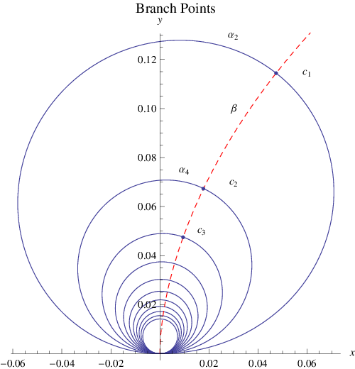
Let $\{c_{n}\}_{n>0}$ be the solutions on the first quadrant, ordered according to decreasing distance from the origin,

|c_{1}|>|c_{2}|>|c_{3}|>\cdots\cdots>|c_{n-1}|>|c_{n}|>|c_{n+1}|>\cdots>0,\,\,\,\,\,\,\,\,\,\,\,\,\,\forall n>1.

(161)

Table 1: Exact and asymptotic values of the first few branch points

c_{n}

’s (of order one) of

h

, together with the convergence radii

R_{n}

’s of the power expansions of the

h_{n}(z)

’s around

z=0

and the convergence radii

\rho_{n}

’s of the semi-integer power expansions around the

c_{n}

’s (see main text).

Branch points of $h(z)$ and related quantities
$n$	$c_{n}$	$c_{n}^{as}$	$R_{n}$	$\rho_{n}$
$1$	$\,0.0473642+i\,0.114414$	$0.0470313+i\,0.114685$	$0.123830$	0.0632582
$2$	$\,0.0177821+i\,0.0673565$	$0.0177176+i\,0.067393$	$0.0696642$	0.0214698
$3$	$\,0.00946886+i\,0.0475615$	$0.0094478+i\,0.0475706$	$0.0484949$	0.0114077

Since eq.(156) has real coefficients, solutions come in pairs of complex-conjugated points and therefore we define

c_{n}\,\equiv\,\overline{c_{-n}}\,\,\,\,\,\,\,\,\,\,\,\,{\rm for}\,\,\,\,\,n<0.

(162)

Exact values for the first few $c_{n}$ ’s are given in the table. An accurate analytic formula (see appendix B) turns out to be:

c_{n}^{as}\,=\,\frac{i}{\pi(2n+1/2)+i\ln\big[e\pi(2n+1/2)\big]-\ln\big[e\pi(2n+1/2)\big]/(\pi(2n+1/2))},\,\,\,\,\,\,\,\,\,\,\,\,\,n\geq 1,

(163)

where “ $\ln$ ” is the logarithm of real analysis. The relative error with respect to the exact value is around $0.3\%$ for $n=1$ and quickly goes to zero for increasing $n$ (see Table 1).

The first derivative of $f(w)$ also vanishes for $u\to-\infty$ , with $w=u+iv$ and $u,v\in{\mathbb{R}}$ . That would suggest that also

z=0=\lim_{u\to-\infty}f(u+iv)

(164)

is a branch point of $h(z)$ . That however is not true because the origin is not an isolated singularity being, as we have just seen, an accumulation point of the order-one branch points.

5.2 The Point at Infinity

Let us now consider the point at infinity. We make the usual change of variable $\zeta\equiv 1/z$ , so that

\zeta=\zeta(u+iv)=\frac{u+iv}{e^{u+iv}-1},

(165)

and study the limit $\zeta\to 0$ . In that limit, $u\to\infty$ and

\frac{d\zeta}{dw}(u+iv)\,=\,\frac{(1-u-iv)\,e^{u+iv}-1}{(e^{u+iv}-1)^{2}}\,\to\,0.

(166)

The point at infinity is therefore a branch point of $h$ . Evaluating the higher-order derivatives of $\zeta(w)$ , one easily finds that they all vanish for $u\to\infty$ , implying that $z=\infty$ is a branch point of infinite order for $h(z)$ . Indeed, for $u\gg 1$ ,

f(u+iv)=\frac{e^{u+iv}-1}{u+iv}\cong\frac{e^{u+iv}}{u+iv}\simeq\frac{e^{u+iv(1-1/u)}}{u}\approx\frac{e^{u+iv}}{u},

(167)

where the last two relations hold for $v\ll u$ , for example $v=\mathcal{O}(1)$ . A sequence of progressively more crude approximations has been generated above, the last one implying that $z=\infty$ should be a logarithmic branch point for $h$ . We will see later that $h(z)$ actually has an infinite-order branch point at $z=\infty$ , originating from a countable set of order-one branch points at infinity, which ”conspire” to produce a singularity resembling a logarithmic branch point.

Since $f(2\pi in)=0$ for any $n\neq 0$ , $f(0)=1$ , and $f^{\prime}(2\pi in)\neq 0$ for any $n$ , local inverses $h_{n}(z)$ do exist because of the inverse function theorem, satisfying

h_{n}(0)=2\pi in\,\,\,\,\,\,\,\,\,\,{\rm for}\,\,\,n\neq 0;\,\,\,\,\,\,\,\,\,\,h_{0}(1)=0.

(168)

We will analytically continue the above branches to properly cut $z$ -planes in the next sections.

5.3 The Branch $h_{0}$

By evaluating both sides of eq.(258) in $z=1$ (see appendix A), one finds that this equation relates $h_{0}$ to the principal branch of the Lambert $W$ function:

h_{0}(z)=\,-\,\frac{1}{z}\,-\,W_{*}\left(-\frac{e^{-1/z}}{z}\right).

(169)

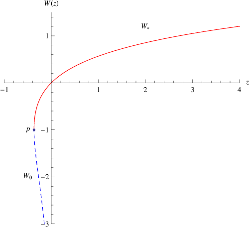
$W_{*}$ has the following series expansion around the origin [14]:

W_{*}(\zeta)=\sum_{n=1}^{\infty}(-1)^{n-1}\frac{n^{n-1}}{n!}\,\zeta^{n},

(170)

which is convergent for

|\zeta|\leq\frac{1}{e}.

(171)

The above one is actually the expansion of the bound-state quantum number $\chi(g)$ for $|g|\ll 1$ , i.e. for a tightly-bounded particle. Since $\exp(-1/c_{n})/c_{n}=1/e$ , by evaluating $h_{0}$ in $c_{n}$ , we obtain

h_{0}(c_{n})=\,-\,\frac{1}{c_{n}}\,-\,W_{*}\left(-\frac{1}{e}\right).

(172)

The numerical series appearing on the r.h.s. can be exactly summed [14]:

\sum_{n=1}^{\infty}\frac{n^{n-1}}{n!\,e^{n}}\,=\,1\,,

(173)

implying that

h_{0}(c_{n})=1\,-\,\frac{1}{c_{n}}=d_{n},

(174)

for any $n\neq 0$ . Therefore we conclude that all the order-one branch points of $h$ lie on the sheet $S_{0}$ , where $h_{0}$ is defined (see fig.9 for a real plot). Since an order-one branch point glues together two different sheets, we have to find the second sheet containing the branch point $c_{n}$ for any given $n\neq 0$ . That is accomplished in the next section.

Another relevant expansion for $h_{0}$ is the one centered in $z=1$ , which is related to the case of the ”loosely bounded particle” discussed before:

h_{0}(z)=\sum_{n=1}^{\infty}k_{n}(z-1)^{n},\,\,\,\,\,\,\,\,\,\,\,\,\,\,\,\,\,\,|z-1|<r,

(175)

where, by Abel’s theorem,

r=\inf_{n\in{\mathbb{Z}}}\left|1-c_{n}\right|=\left|1-c_{1}\right|\cong 0.959482.

(176)

The first few coefficients explicitly read:

$\displaystyle k_{1}$	$\displaystyle=$	$\displaystyle+2;$	(177)
$\displaystyle k_{2}$	$\displaystyle=$	$\displaystyle-\frac{4}{3};$	(178)
$\displaystyle k_{3}$	$\displaystyle=$	$\displaystyle+\frac{10}{9}.$	(179)

5.4 The Branches $h_{n}$ for $n\neq 0$

By evaluating a large number of terms (up to $10^{3}$ ) in the power-expansion of $h_{n}(z)$ around $z=0$ for various $n=1,2,3,\cdots$ ,

h_{n}(z)=\sum_{k=0}^{\infty}a_{k}^{(n)}z^{k},\,\,\,\,\,\,\,\,\,|z|<R_{n},

(180)

and using the standard convergence tests, we find that

R_{n}=|c_{n}|\,\approx\,\frac{1}{2\pi|n|}

(181)

for any $n\neq 0$ . Let us remark that eq.(180) is actually the perturbative expansion of $k^{(n)}(g)$ in powers of $g$ given in eq.(126) in a different notation, so we do not repeat the values of the lowest-order coefficients. Since the $c_{n}$ ’s are ordered according to their modulus (see eq.(161)), we conclude that the sheet $S_{1}$ only has the branch point $c_{1}$ (plus an order-one branch point at infinity), $S_{2}$ has only the branch point $c_{2}$ and so on. Therefore:

h_{n}(c_{n})=h_{0}(c_{n})=d_{n}=1-\frac{1}{c_{n}},\,\,\,\,\,\,\,\,\,\,n\neq 0

(182)

while

h_{k}(c_{n})\neq d_{n}\,\,\,\,\,\,\,\,\,\,\,{\rm for}\,\,\,\,\,\,k\neq n.

(183)

The branch point $c_{n}$ then glues together the sheet $S_{n}$ to $S_{0}$ for any $n\neq 0$ .

5.5 Expansions Around the Branch Points $c_{n}$ ’s

In this section we present an expansion of $h(z)$ around the branch point $c_{n}$ for some fixed $n\neq 0$ . Since the latter is an order-one branch point, the series involves semi-integer powers of $z-c_{n}$ . The expansion is obtained by inverting the Taylor series of $z=f(w)$ around $d_{n}$ , with $c_{n}=f(d_{n})$ ,

z-c_{n}=\sum_{k=2}^{\infty}\frac{f^{(k)}(d_{n})}{k!}(w-d_{n})^{k}.

(184)

We replace on the r.h.s. of the above equation the semi-integer power (Puiseaux) expansion

w-d_{n}=\sum_{l=1}^{\infty}b_{l}^{(n)}\,(z-c_{n})^{l/2},

(185)

expand everything in powers of $z-c_{n}$ and determine the coefficients $b_{l}^{(n)}$ in such a way that equality holds order by order in $z-c_{n}$ [20]¹⁷¹⁷ 17 This method is a generalization to the case $f^{\prime}(d_{n})=0$ of the standard series inversion.. For the first few orders, for example, we have the explicit expressions:

$\displaystyle b_{1}^{(n)}$	$\displaystyle=$	$\displaystyle\frac{1}{\sqrt{a_{2}^{(n)}}};$	(186)
$\displaystyle b_{2}^{(n)}$	$\displaystyle=$	$\displaystyle-\frac{a_{3}^{(n)}}{2\left(a_{2}^{(n)}\right)^{2}};$	(187)
$\displaystyle b_{3}^{(n)}$	$\displaystyle=$	$\displaystyle\frac{5\left(a_{3}^{(n)}\right)^{2}-4a_{2}^{(n)}a_{4}^{(n)}}{8\left(a_{2}^{(n)}\right)^{3}\sqrt{a_{2}^{(n)}}},$	(188)

where we have defined

a_{k}^{(n)}\equiv\frac{f^{(k)}(d_{n})}{k!}\,\,\,\,\,\,\,\,\,\,\,(k\geq 2).

(189)

By $\sqrt{a_{2}^{(n)}}$ we mean an arbitrary but fixed complex square root of $a_{2}^{(n)}$ , for example the branch with $-\pi<\arg z\leq\pi$ ( $1^{1/2}=1)$ . Changing the convention for $\sqrt{a_{2}^{(n)}}$ is equivalent to go from one determination of $(z-c_{n})^{1/2}$ to the other.

To summarize, we have the expansion

h_{n,0}(z)=d_{n}+\sum_{k=1}^{\infty}b_{k}^{(n)}\,(z-c_{n})^{k/2}.

(190)

The double subscript is to remember that the expansion allows to compute the values of both branches $h_{n}(z)$ and $h_{0}(z)$ for $z$ sufficiently close to $c_{n}$ . The above series, by a generalization of Abel’s theorem, is convergent up to the closest singularity to $c_{n}$ in the $z$ -plane,

|z-c_{n}|<\rho_{n}\,=\,\min\Big\{|c_{n}-c_{n-1}|,\,|c_{n}-c_{n+1}|\Big\}\,=\,|c_{n}-c_{n+1}|,\,\,\,\,\,\,\,\,\,\,\,{\rm for}\,\,\,n>1,

(191)

with $\rho_{1}=|c_{1}-c_{2}|$ and $\rho_{-n}=\rho_{n}$ for $n<0$ . Exact values for the first few $\rho_{n}$ ’s are given in the table. Asymptotically:

\rho_{n}\simeq\frac{1}{2\pi\,n(n+1)},

(192)

for $n\gg 1$ . Let us remark that $\rho_{n}>0$ for any $n\neq 0$ , but tends to zero for $n\to\pm\infty$ .

5.6 Matching Different Expansions

In this section, in order to check the analytic-geometric structure of the function $h$ previously established, we match the different expansions obtained.

Let us denote with $D\subseteq{\mathbb{C}}_{z}$ the convergence region of the expansion of $h_{0}(z)$ coming from the power expansion in zero of $W_{*}$ ,

D\equiv\big\{z\in{\mathbb{C}}\backslash\{0\}:|\exp(-1/z)/z|\leq 1/e\big\},

(193)

with $B\left(0;\,R_{n}\right)$ the convergence disk of the expansion of $h_{n}(z)$ around $0$ ,

B\left(0;\,R_{n}\right)\equiv\big\{z\in{\mathbb{C}}:|z|<R_{n}\big\},

(194)

and by $B\left(c_{n};\,\rho_{n}\right)$ the convergence disk of the semi-integer expansion of $h_{n,0}(z)$ in $c_{n}$ derived above (see fig.10),

B\left(c_{n};\,\rho_{n}\right)\equiv\big\{z\in{\mathbb{C}}:|z-c_{n}|<\rho_{n}\big\}.

(195)

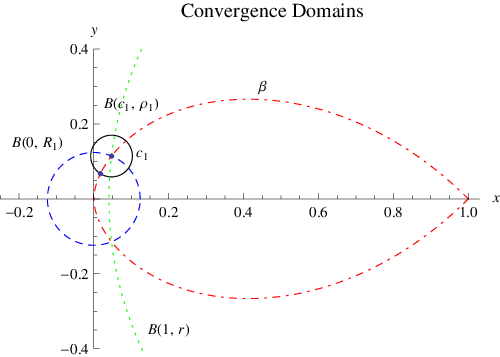
We can pick up any point $p$ in the double intersection

p\in D\cap B\left(c_{n};\,\rho_{n}\right)

(196)

and fix the sign of $\sqrt{a_{2}^{(n)}}$ in such a way that, for example,

h_{n,0}(p)=+h_{0}(p).

(197)

Because of continuity, the sign is constant on any connected component of the intersection above. Since the latter is connected, being $D$ and $B\left(c_{n},\rho_{n}\right)$ convex, the sign is unique. Then for every point

q\in B\left(0;\,R_{n}\right)\cap B\left(c_{n};\,\rho_{n}\right),

(198)

it must hold

h_{n,0}(q)=-h_{n}(q),

(199)

since similar considerations as those above for the sign also hold in this case. Other checks of the analytic structure of $h$ can be obtained by considering the power-expansion in $z-1$ of $h_{0}$ discussed previously, or by taking into account that

B\left(c_{n};\rho_{n}\right)\cap B\left(c_{n+1},\rho_{n+1}\right)\neq\emptyset,\,\,\,\,\,\,\,\,\,n\geq 1.

(200)

Since $B\left(c_{n};\rho_{n}\right)\cap B\left(c_{n+2},\rho_{n+2}\right)=\emptyset$ , one has to proceed through a chain of disks. In general, one can analytically continue the function $w=h(z)$ by moving along paths in the $z$ -plane with the ODE derived in the next section or by means of the standard Weierstrass procedure involving a sequence of overlapping circles [21].

5.7 Cuts

We cut the $z$ -plane of the function $h$ along curves $t_{n}$ starting from the branch points $c_{n}$ and going to $-\infty$ , of the (arbitrarily chosen) form

z_{n}(t)=a_{n}-t+i\frac{b_{n}}{1+t},\,\,\,\,\,\,\,\,\,\,t\geq 0,

(201)

where $c_{n}=a_{n}+ib_{n}$ with $a_{n},b_{n}\in{\mathbb{R}}$ , $n\neq 0$ . In fig.11 we plot the $z$ -plane cut along $t_{1}$ , i.e. the sheet $S_{1}$ where the branch $h_{1}$ is defined, while in fig.12 we plot the sheet $S_{0}$ , where the branch $h_{0}(z)$ is defined, having all the cuts $t_{n}$ , $n\neq 0$ .

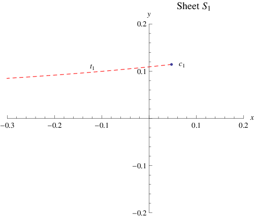
The lifted curves $T_{n}$ in the $w$ -plane are obtained by integrating numerically the ordinary differential equation (ODE) for $w=h(z)$ ,

\frac{dw}{dz}=\frac{w}{z\,w-z+1},

(202)

along $t_{n}$ .

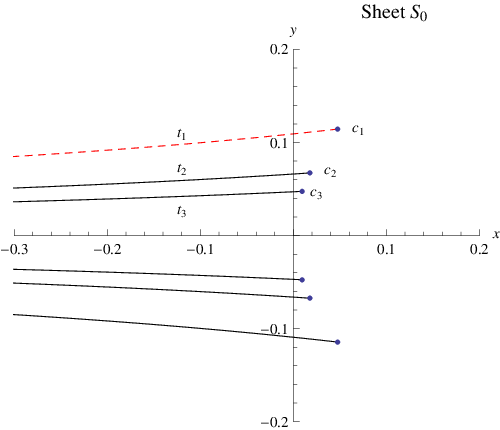
A singularity of the solution is expected when the denominator, a polynomial of second degree in $z$ and $w$ , vanishes [22], i.e. when:

w=1-\frac{1}{z}.

(203)

The above equation, combined with the relation between $w$ and $z$ provided by eq.(152), gives the equation for the branch points already obtained

e^{1-1/z}=z.

(204)

By selecting one determination for the function $h$ , let us define

w_{n}(t)\equiv w\left(z_{n}(t)\right).

(205)

The ODE for $T_{n}$ explicitly reads:

\frac{dw_{n}}{dt}(t)=\frac{w_{n}(t)}{z_{n}(t)\,w_{n}(t)-z_{n}(t)+1}\,\frac{dz_{n}}{dt}(t).

(206)

It is clear that an initial condition to the above ODE for $w_{n}(t)$ cannot be provided at $t=0$ : solution could not be unique as we would “begin to move” starting from a branch point:

w_{n}(0)=d_{n},\,\,\,\,\,\,z_{n}(0)=c_{n}.

(207)

As we have just shown, $dw/dz$ , as given by the r.h.s. of eq.(202), formally diverges for $z\to c_{n}$ and $w\to d_{n}$ . We therefore solve the ODE for $t\geq t_{0}$ with $0<t_{0}\ll 1$ ¹⁸¹⁸ 18 We see here, in a differentiable context, the (algebraic topology) theorem of the unicity of lifted paths, once an element in the preimage of a point in the base curve is chosen [23]. . The initial condition $w_{n}(t_{0})$ can be derived by means of the semi-integer expansion (190)

w_{n}\left(t_{0}\right)=d_{n}+\sum_{k=1}^{\infty}b_{k}^{(n)}\,\big(z_{n}(t_{0})-c_{n}\big)^{k/2}.

(208)

For each $z_{n}(t_{0})$ , there are two $w_{n}(t_{0})$ ’s because of the square root terms, as it should for an order-one branch point. The two different initial conditions correspond to the two sides of the cut one is moving along to.

In practice, to obtain a high accuracy, one has to compromise about the numerical value of $t_{0}>0$ . On the one hand, $t_{0}$ has to be quite close to zero in such a way that $z_{n}(t_{0})-c_{n}$ is so small that the series expansion above converges quickly, while on the other hand $t_{0}$ has to be large enough so that $dw/dz$ is not too big in the first iterations of the ODE.

5.8 Asymptotic Expansions

For $|\ln_{n}(z)|\gg 1$ , the following asymptotic expansion holds:

h_{n}(z)=\ln_{n}(z)+\ln_{0}\left[\ln_{n}(z)\right]+\frac{\ln_{0}\left[\ln_{n}(z)\right]}{\ln_{n}(z)}+\frac{1}{z\ln_{n}(z)}+\mathcal{O}\left[\frac{1}{\ln_{n}^{2}(z)}\right],

(209)

where by $\ln_{n}(z)$ we mean the branch of $\ln(z)$ with argument $\arg_{n}$ , in the range

\pi(2n-1)<\arg_{n}(z)<\pi(2n+1),\,\,\,\,\,\,\,\,\,\,\,\,n\in{\mathbb{Z}}.

(210)

The dependence on $n$ can be made explicit as:

\ln_{n}(z)=\ln_{0}(z)+2\pi in.

(211)

For the ”external” logarithm, we have (conventionally) taken the principal branch $\ln_{0}[\cdots]$ ; one can actually choose any other branch, as the difference between different choices cancels order by order in the expansion, as proved in appendix C. An important point is that $\ln_{n}(z)$ becomes large in two quite different situations:

1.

$|z|\gg 1$ , any $n$ . This case is related to the strong-coupling regime of the Winter model;¹⁹¹⁹ 19 The case $|z|\ll 1$ must be discarded because $z=0$ , as we have seen before, is a non-isolated singularity of $h$ , so no expansion around the origin of the above form exists.
2.

$|n|\gg 1$ , any $z\neq 0$ . This case is related to the high-energy excitations of Winter model in the weak-coupling regime, which is our main concern.

Actually, in case 1. one can drop the term proportional to $1/z$ , as it is exponentially small compared to the other ones, so for $|z|\gg 1$ , any $n$ , one has:

h_{n}(z)=\ln_{n}(z)+\ln_{0}\left[\ln_{n}(z)\right]+\frac{\ln_{0}\left[\ln_{n}(z)\right]}{\ln_{n}(z)}+\mathcal{O}\left[\frac{1}{\ln_{n}^{2}(z)}\right].

(212)

For physics applications (see next section), one needs the asymptotic expansion for a real argument. For $x>0$ , the expansion explicitly reads:

	$\displaystyle h_{n}(x)$	$\displaystyle=$	$\displaystyle\ln(x)+2\pi in+\ln_{0}\left[\ln(x)+2\pi in\right]+\frac{\ln_{0}\left[\ln(x)+2\pi in\right]}{\ln(x)+2\pi in}+$		(213)
			$\displaystyle\,\,\,\,\,\,\,\,\,\,\,\,\,\,\,\,\,\,\,\,\,\,\,\,\,\,\,\,\,\,\,\,\,\,\,+\frac{1}{x\big[\ln(x)+2\pi in\big]}+\mathcal{O}\left[\frac{1}{\ln_{n}^{2}(x)}\right],$		(213)

where $\ln(x)$ is the real logarithm of $x>0$ . As in the general case above, for $x\gg 1$ , any $n$ , one drops the power-suppressed term proportional to $1/x$ . The argument $2\pi n$ entering the above formula can be directly obtained by considering the curve in the $w$ -plane (see the dashed (blue) lines to the right of the imaginary axis in fig.13):

\Gamma_{n}:\,\,\,w=w_{n}(u)=u+2\pi in,\,\,\,\,\,u\geq 0.

(214)

For $n\neq 0$ , by taking the formal inverse of $f(w_{n}(0))=0$ , we obtain $h(0)=w_{n}(0)=2\pi in$ , implying that we are on the branch $n$ at the initial point of $\Gamma_{n}$ : $h=h_{n}$ . As shown previously, for $u\gg 1$ ,

f(w_{n}(u))\approx\frac{e^{u}}{u}.

(215)

We now take the inverse again, of the above formula. Since the curve $\Gamma_{n}$ does not cross the preimage $T_{n}$ of the cut $t_{n}$ in $S_{n}$ , it is entirely contained in $h_{n}(S_{n})$ . By continuity therefore the inverse is again $h_{n}$ and $u+2\pi in\approx h_{n}(e^{u}/u)$ . With $x=e^{u}/u$ , we then obtain $h_{n}(x)\approx\ln(x)+2\pi in$ . For $n=0$ the argument is similar: one takes the inverse of $f(w_{0}(0))=1$ and gets the branch $h_{0}$ ; again, the curve $\Gamma_{0}$ does not cross any of the curves $T_{n}$ , so it is entirely contained in $h_{0}(S_{0})$ . For

x>0\,\,\,\,\,\,\,\,\,\,\,{\rm and}\,\,\,\,\,\,\,n\gg\frac{1}{2\pi x},

(216)

the desired expansion reads:

	$\displaystyle h_{n}(x)$	$\displaystyle=$	$\displaystyle 2\pi i\left(n+\frac{1}{4}\right)+\ln\left[2\pi\left(n+\frac{1}{4}\right)x\right]-i\,\frac{\ln\Big[2\pi(n+1/4)x\Big]}{2\pi(n+1/4)}+$		(217)
			$\displaystyle\,\,\,\,\,\,\,\,\,\,\,\,\,\,\,\,\,\,\,\,\,-\frac{i}{2\pi(n+1/4)\,x}+\mathcal{O}\left\{\frac{1}{\left[2\pi(n+1/4)\right]^{2}}\right\}.$		(217)

For $n<0$ , one just takes the complex conjugate as:

h_{n}(x)\,=\,\overline{h_{-n}(x)}.

(218)

For $x<0$ , the logarithmic expansion on the r.h.s. of eq.(209) takes the form:

	$\displaystyle h_{n}(x)$	$\displaystyle=$	$\displaystyle\ln\|x\|+i\pi(2n-1)+\ln_{0}\left[\ln\|x\|+i\pi(2n-1)\right]+\frac{\ln_{0}\big[\ln\|x\|+i\pi(2n-1)\big]}{\ln\|x\|+i\pi(2n-1)}+$		(219)
			$\displaystyle\,\,\,\,\,\,\,\,\,\,\,\,\,\,\,\,\,\,\,\,\,\,\,\,\,\,\,\,\,\,+\frac{1}{x\big[\ln\|x\|+i\pi(2n-1)\big]}+\mathcal{O}\left[\frac{1}{\ln_{n}^{2}(x)}\right].$		(219)

As in the previous cases, for $x\ll-1$ and $n\geq 1$ , one drops the power-suppressed term. The determination of the argument $\pi(2n-1)$ in eq.(219) has been obtained by integrating numerically eq.(202) along the negative axis, i.e. for $z=-t$ with $t\geq 0$ with the initial condition $w(0)=2\pi in$ . Let us remark that one cannot evaluate $h_{0}(x)$ for $x<0$ by integrating the ODE for $dw/dz$ starting from $x=0$ because, as we have shown, the origin is a non-isolated singularity for this branch and therefore cannot be used as initial condition. One cannot even start, for example, from $x=1$ ( $h_{0}(1)=0$ ), because one cannot pass through the origin either. Actually, in the latter case, the following instability occurs. By departing arbitrarily small from the real axis, a branch cut $t_{n}$ of some $c_{n}$ is necessarily hit, because the $c_{n}$ ’s accumulate at the origin. As a consequence, one leaves the sheet $S_{0}$ and enters the sheet $S_{n}$ , for some large $n$ , and presumably remains in that sheet, as $S_{n}$ has $c_{n}$ as its only branch point (apart from the point at infinity). The consequence is that there is a not a well-defined value of $h_{0}(x)$ for $x<0$ as far as ”physics” (which deals with $x\in{\mathbb{R}}$ only) is concerned. One has instead to move along great half-circles, starting from positive arguments, ending up with a sign depending on the contour orientation. For

x<0\,\,\,\,\,\,\,\,\,{\rm and}\,\,\,\,\,\,n\gg\frac{1}{2\pi|x|},

(220)

the required expansion explicitly reads:

	$\displaystyle h_{n}(x)$	$\displaystyle=$	$\displaystyle 2\pi i\left(n-\frac{1}{4}\right)+\ln\left[2\pi\left(n-\frac{1}{4}\right)\|x\|\right]-i\,\frac{\ln\Big[2\pi(n-1/4)\|x\|\Big]}{2\pi(n-1/4)}+$		(221)
			$\displaystyle\,\,\,\,\,\,\,\,\,\,\,\,\,\,\,\,\,\,\,\,\,\,\,\,-\frac{i}{2\pi(n-1/4)\,x}\,+\,\mathcal{O}\left\{\frac{1}{\left[2\pi(n-1/4)\right]^{2}}\right\}.$		(221)

Because of the symmetry between eqs.(217) and (221), one can write both equations in a unique form. For

x\in{\mathbb{R}}\backslash\{0\},\,\,\,\,\,\,\,\,n\gg\frac{1}{2\pi|x|},

(222)

it holds:

	$\displaystyle h_{n}(x)$	$\displaystyle=$	$\displaystyle 2\pi i\left(n+\frac{\mathrm{sign}(x)}{4}\right)+\ln\left[2\pi\left(n+\frac{\mathrm{sign}(x)}{4}\right)\|x\|\right]-i\,\frac{\ln\Big[2\pi(n+\mathrm{sign}(x)/4)\|x\|\Big]}{2\pi(n+\mathrm{sign}(x)/4)}+$		(223)
			$\displaystyle\,\,\,\,\,\,\,\,\,\,\,\,\,\,\,\,\,\,\,\,\,-\frac{i}{2\pi(n+\mathrm{sign}(x)/4)\,x}+\mathcal{O}\left\{\frac{1}{\left[2\pi(n+\mathrm{sign}(x)/4)\right]^{2}}\right\},$		(223)

where $\mathrm{sign}(x)=1$ for $x>0$ and $-1$ otherwise is the function, which returns the sign of $x$ .

5.9 Riemann Surface

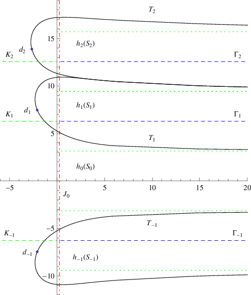
By taking into account the results of the previous sections, one finds that the Riemann surface $S$ of $h$ is constructed by gluing diagonally the borders of the cut $t_{n}$ from $c_{n}$ to $-\infty$ in $S_{n}$ to the corresponding ones in $S_{0}$ , for any $n\neq 0$ ²⁰²⁰ 20 That is exactly what we do with the $z^{1/2}$ function.. Topologically, $S$ is a plane, as it is usually the case with non-compact Riemann surfaces [24, 25]. The images of the branches $h_{n}(S_{n})$ in the $w$ -plane, the total space of the (branched) covering realized by $f$ , are shown in fig.13.

One can visit the entire Riemann surface $S$ by moving along the following simple paths, which are also shown in fig.13. As we have already seen, the dashed (blue) horizontal line on the right half-plane of $w$ ,

\Gamma_{n}:\,\,\,w=w_{n}(u)=u+2\pi in,\,\,\,\,\,\,u\geq 0,

(224)

does not cross any continuous (black) curve $T_{n}$ , passing through $d_{n}$ , which is the preimage under $h$ of the cut $t_{n}$ . $\Gamma_{n}$ is therefore completely contained in $h_{n}(S_{n})$ . Let us remark that the point $d_{n}$ divides the curve $T_{n}$ into two arcs, each of which is mapped by $f$ onto $t_{n}$ ²¹²¹ 21 It’s like with the function $w=z^{1/2}$ , where the origin of the $z$ -plane divides any line passing through it into two half-lines, each of which is mapped onto the same half-line of the $w$ -plane.. As already discussed, these ”intra-sheet” paths $\Gamma_{n}$ allow one to connect the power expansion of $h_{n}(z)$ in $z=0$ with the logarithmic expansion at $z=\infty$ . The dashed horizontal (green) line on the left half of the $w$ plane,

K_{n}:\,\,\,w=w_{n}(u)=u+2\pi in,\,\,\,\,\,\,u\leq 0,\,\,\,n\neq 0,

(225)

crosses the continuous (black) curve $T_{n}$ once and therefore allows one to go from the sheet $n$ to the sheet $0$ (or viceversa):

K_{n}:\,\,\,\,S_{n}\leftrightarrow S_{0}.

(226)

The image curves $k_{n}=f(K_{n})$ in the base space $z$ are shown still dashed (in green) in fig.14.

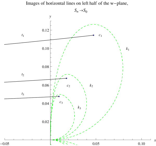
The dotted-dashed (red) vertical line,

J_{k}:\,\,\,w=w_{k}(v)=k+iv,\,\,\,\,\,\,v\in{\mathbb{R}},

(227)

where $k$ is a real constant, crosses all the $T_{n}$ ’s for $k\raisebox{-3.0pt}{$\>\stackrel{{\scriptstyle>}}{{\scriptstyle\sim}}\>$}{\rm Re}\,d_{1}$ , and allows one to go from $S_{n}$ to $S_{n+1}$ via $S_{0}$ :

J_{k}:\,\,\,S_{n}\leftrightarrow S_{0}\leftrightarrow S_{n+1},\,\,\,\,\,\,(n\neq 0;\,k\raisebox{-3.0pt}{$\>\stackrel{{\scriptstyle>}}{{\scriptstyle\sim}}\>$}{\rm Re}\,d_{1}).

(228)

For $k\gg 1$ , the image curve in the base space $j_{k}=f(J_{k})$ is basically a great spiral winding an infinite number of times around the point $z=\infty$ , which we have proven to be an infinite-order branch point for $h$ . For $k\ll{\rm Re}\,d_{1}$ only some sheets are visited; in this case one can still go from any $S_{n}$ to $S_{n+1}$ by passing though $S_{0}$ via the dashed (green) lines. $J_{0}$ coincides with the imaginary axis of the $w$ -plane, its image in the base space $j_{0}=f(J_{0})$ contains the curves $\alpha_{n}$ ’s considered in appendix B (see eq.(271)) and passes through the origin $z=0$ an infinite number of times. Closed curves are obtained in this case and all the multivaluedness of $h$ is seen in a very clean way. For $n\neq 0$ , one has indeed $f(w_{0}(n))=0$ , implying $h_{n}(0)=2\pi in=w_{0}(n)$ , while $f(w_{0}(0))=1$ implies $h_{0}(1)=0=w_{0}(0)$ . A portion of the image curve $j_{0}=f(J_{0})$ in the base space is shown, again dotted-dashed (in red), in fig.15

6 Non-Perturbative Analysis

This is the central section of the paper, in which the limits of perturbation theory are rigorously established, non-perturbative results for various observables are obtained and compared with the perturbative formulas. The perturbative results for frequencies, widths and mixing matrix elements of resonances have all been obtained by inserting into the exact expressions the power expansions for $k^{(n)}(g)=n-ng+\cdots$ , which converge only for

|g|\,\leq\,R_{n}\,\approx\,\frac{1}{2\pi n}.

(229)

Therefore, if we consider a fixed resonance (i.e. if we fix $n$ ), its properties can be analyzed with arbitrary accuracy by means of the perturbative formulas for small enough $|g|$ . Actually, we are interested in varying $n$ within a specified model, i.e. at fixed $g$ ; by inverting the above inequality, the following upper bound on $n$ is obtained:

n\,\raisebox{-3.0pt}{$\>\stackrel{{\scriptstyle<}}{{\scriptstyle\sim}}\>$}\,\frac{1}{2\pi|g|}.

(230)

Therefore at fixed $g\ll 1$ (”fixed physics”), only the resonances satisfying the above inequality can be described by means of perturbation theory.

In order to obtain non-perturbative results, we basically insert in the general formulas for the observables, the large- $n$ expansion previously obtained, which we repeat here for easy of reference:

	$\displaystyle h_{n}(-g)$	$\displaystyle=$	$\displaystyle 2\pi i\left(n-\frac{\mathrm{sign}(g)}{4}\right)+\ln\left[2\pi\left(n-\frac{\mathrm{sign}(g)}{4}\right)\|g\|\right]-i\,\frac{\ln\Big[2\pi(n-\mathrm{sign}(g)/4)\|g\|\Big]}{2\pi(n-\mathrm{sign}(g)/4)}+$		(231)
			$\displaystyle\,\,\,\,\,\,\,\,\,\,\,\,\,\,\,\,\,\,\,\,\,+\frac{i}{2\pi(n-\mathrm{sign}(g)/4)\,g}+\mathcal{O}\left\{\frac{1}{\left[2\pi(n-\mathrm{sign}(g)/4)\right]^{2}}\right\},$		(231)

where $\mathrm{sign}(g)$ is the function which returns the sign of $g$ . The basic equation, which replaces the perturbative formula given in eq.(126) valid for small $n$ , reads:

$\displaystyle k^{(n)}(g)$	$\displaystyle=$	$\displaystyle\frac{h_{n}(-g)}{2\pi i}$	(232)
	$\displaystyle=$	$\displaystyle n-\frac{\mathrm{sign}(g)}{4}-\frac{i}{2\pi}\,\ln\left\{2\pi\|g\|\left[n-\frac{\mathrm{sign}(g)}{4}\right]\right\}-\,\frac{\ln\Big\{2\pi\|g\|\,\big[n-\mathrm{sign}(g)/4\big]\Big\}}{4\pi^{2}\big[n-\mathrm{sign}(g)/4\big]}+$
		$\displaystyle\,\,\,\,\,\,\,\,+\frac{1}{4\pi^{2}\,g\,\big[n-\mathrm{sign}(g)/4\big]}\,+\,\mathcal{O}\left\{\frac{1}{\left[2\pi(n-\mathrm{sign}(g)/4)\right]^{2}}\right\}.$

The expansion begins with $n$ in both cases but, while the perturbative expansion is an expansion in powers of $g$ , the non-perturbative one is basically an expansion in powers of $1/n$ . For

0<|g|\ll 1\,\,\,\,\,\,\,\,\,\,{\rm and}\,\,\,\,\,\,\,n\gg\frac{1}{2\pi|g|},

(233)

the frequencies and the widths take the form:

	$\displaystyle\omega^{(n)}(g)$	$\displaystyle=$	$\displaystyle n^{2}-\frac{\mathrm{sign}(g)}{2}n+\mathcal{O}(1),$		(234)
	$\displaystyle\Gamma^{(n)}(g)$	$\displaystyle=$	$\displaystyle\frac{2}{\pi}\,n\ln\big[2\pi\|g\|n\big]+\mathcal{O}(1).$		(235)

By comparing with the perturbative results obtained previously, we see that the frequencies have a similar dependence on $n$ to the free case, while the widths grow much less with increasing $n$ .

Since we do not manipulate perturbative formulas in this section, there is no more convenience in introducing renormalization constants and renormalized mixing matrices for the resonances, so we switch back to the original (unrenormalized) mixing matrix $V(g)$ and resonances $\theta_{n}$ . In terms of the function $h$ , the entries of the mixing matrix $V(g)$ read for large $n$ :

	$\displaystyle V(g)_{l,n}$	$\displaystyle=$	$\displaystyle(-1)^{l+1}\,2lg\,\frac{k^{(n)}(g)}{k^{(n)}(g)^{2}-l^{2}}\,\frac{e^{1/2\,h_{n}(-g)}}{e^{h_{n}(-g)}+g}$		(236)
		$\displaystyle=$	$\displaystyle(-1)^{l+1}\,2lg\,\frac{k^{(n)}(g)}{k^{(n)}(g)^{2}-l^{2}}\,e^{-1/2\,h_{n}(-g)}\left[1-ge^{-h_{n}(-g)}+g^{2}e^{-2h_{n}(-g)}+\cdots\right].$		(236)

By inserting the previous expansion for $h_{n}(-g)$ , the matrix elements take the explicit form:

V(g)_{l,n}=\sqrt{\frac{2}{\pi}}\,\mathrm{sign}(g)\,e^{i\pi/4\,\mathrm{sign}(g)}\,\frac{(-1)^{l+n+1}l\sqrt{|g|\,n}}{n^{2}-i\,n\log\big[2\pi|g|n\big]/\pi-\mathrm{sign}(g)\,n/2-l^{2}}\left[1+\mathcal{O}\left(\frac{1}{n}\right)\right]\,.

(237)

A few comments are in order: 1) higher-order corrections in $1/n$ can be computed in a straightforward way; 2) the alternating sign $(-1)^{n}$ is present both in the small- $n$ and large- $n$ expansions of $V(g)_{l,n}$ : it is related to the logarithmic behavior of the function $h$ at infinity. As we have seen in the previous section, this factor is also present in the inverse of the perturbative expression for $V(g)$ , i.e. in $V_{\rm pt}(g)^{-1}$ . We expect a similar phenomenon to occur also in the exact inverse. Indeed, by looking for example at eq.(148), one notices that the alternating sign $(-1)^{n}$ produces constructive interference of the harmonics entering the sine Fourier transform around $x=\pi$ , which is the region where non-trivial dynamics occurs. For $n\gg l$ with fixed $l$ , i.e. along a row well to the right to the main diagonal,

V(g)_{l,n}\simeq\sqrt{\frac{2}{\pi}}\,\mathrm{sign}(g)\,e^{i\pi/4\,\mathrm{sign}(g)}\,\,\sqrt{|g|}\,\,\frac{(-1)^{l+n+1}l}{n^{3/2}},\,\,\,\,\,\,\,\,\,\,\,\,\,\,\,\,\,\,\,\,\,n\gg l.

(238)

Therefore, for large $n$ there is a rather slow power-law decay, with the alternating sign $(-1)^{n}$ . The above behavior has to be compared with the perturbative one: as we have seen, $V(g)_{l,n}\approx 1/n$ to $\mathcal{O}(g)$ , with convergence properties deteriorating in second order: $V(g)_{l,n}\approx 1$ to $\mathcal{O}\left(g^{2}\right)$ . For $l\gg n$ , i.e. along a column well below the main diagonal:

V(g)_{l,n}\simeq\sqrt{\frac{2}{\pi}}\,\mathrm{sign}(g)\,e^{i\pi/4\,\mathrm{sign}(g)}\,\frac{(-1)^{l+n}\,\sqrt{|g|\,n}}{l},\,\,\,\,\,\,\,\,\,\,\,\,\,\,\,\,\,l\gg n.

(239)

A quite slow inverse-power decay with $l$ occurs, with an alternating sign, exactly as in the perturbative case. Finally, on the diagonal, one explicitly has:

V(g)_{n,n}\,=\,e^{-i\pi/4\,\mathrm{sign}(g)}\,\frac{\sqrt{2\pi|g|n}}{\ln\big(2\pi|g|n\big)-i\pi\mathrm{sign}(g)/2}\left[1+\mathcal{O}\left(\frac{1}{n}\right)\right],\,\,\,\,\,\,\,\,\,\,\,\,\,\,\,\,l=n.

(240)

Therefore, for large $n$ a square-root divergence basically occurs. In perturbation theory we found instead $V_{n,n}\approx 1$ to $\mathcal{O}(g)$ and $V_{n,n}\approx n$ to $\mathcal{O}\left(g^{2}\right)$ (to see that just invert eq.(125) with respect to $V(g)$ or see [6]).

A numerical analysis (involving the inversion of matrices of various order up to $2\times 10^{4}$ ) shows that

\left|\left(V(g)^{-1}\right)_{l,n}\right|\,\approx\,\frac{1}{n};\,\,\,\,\,\,\,\,\,\,\,\,\arg\left[\left(V(g)^{-1}\right)_{l,n+1}\right]-\arg\left[\left(V(g)^{-1}\right)_{l,n}\right]\,\approx\,\pi\,\,\,\,\,\,\,\,\,\,\,\mathrm{for}\,\,\,\,n\gg l.

(241)

The first relation implies that it is not possible to excite exactly one resonance at a time by means of a sensible (i.e. belonging to $H^{1}\left({\mathbb{R}}^{+}\right)$ ) initial wavefunction and one has necessarily to use the approximate (truncated) scheme. Note that

\theta(\pi-x)\sum_{n=1}^{\infty}\frac{(-1)^{n+1}}{n}\sin(nx)\,=\,\theta(\pi-x)\frac{x}{2}.

(242)

We can summarize the above findings by saying that an exact treatment of $V(g)^{-1}$ only partially regularizes the perturbative results. The inverse matrix elements $\left(V(g)^{-1}\right)_{l,n}$ in the non-perturbative case decay faster for $n\to\infty$ than in the perturbative case, giving rise to less singular initial data.

7 Conclusions

The resonances of the Winter model in the weak coupling domain $0<|g|\ll 1$ — which is the most interesting one — are subjected to two different regimes. The first one is the perturbative one, accurately describing the dynamical properties of the $n$ -th resonance up to

n\,\raisebox{-3.0pt}{$\>\stackrel{{\scriptstyle<}}{{\scriptstyle\sim}}\>$}\,\frac{1}{2\pi|g|}.

(243)

The second regime is non-perturbative in character and describes the dynamics of the $n$ -th resonance for

n\,\gg\,\frac{1}{2\pi|g|}.

(244)

Actually, there is also an intermediate region,

n\,\approx\,\frac{1}{2\pi|g|},

(245)

which, contrary to the above ones, cannot be described by simple analytic formulas. In physical terms, we may say that perturbation theory accurately describes the low-energy excitations of the model, while it completely fails to describe the high-energy ones ( $|g|\ll 1$ always). For the decay widths of resonances, for example, we found:

\Gamma^{(n)}(g)\,\simeq\,\left\{\begin{array}[]{cc}4\pi g^{2}n^{3}\,+\,\mathcal{O}(g^{3})\,\,\,\,\,\,\,\,\,\,\,\,\,\,\,\,\,\,\,\,\,\,\,\,\,{\rm for}\,\,n\raisebox{-3.0pt}{$\>\stackrel{{\scriptstyle<}}{{\scriptstyle\sim}}\>$}1/(2\pi|g|)\,;\\ 2/\pi\,n\ln\big(2\pi|g|n\big)\,+\,\mathcal{O}(1)\,\,\,\,\,\,{\rm for}\,\,n\gg 1/(2\pi|g|)\,.\end{array}\right.

(246)

The growth of the widths with $n$ is strongly reduced for large $n$ ,

n^{3}\,\to\,n\ln n,

(247)

so that the extrapolation of the perturbative formula above in the high-energy region would produce completely wrong results. We have also provided explicit non-perturbative expressions for some physically relevant quantities, such as wavevectors, frequencies and mixing-matrix entries of resonances, which replace the perturbative formulas previously obtained [5, 6]. We have shown that it is not possible to construct in perturbation theory initial wavefunctions exciting exactly one resonance at a time. By inverting numerically the exact matrix $V(g)$ truncated up to order $N\approx 2\times 10^{4}$ , we have found that that is not even possible to construct such a wavefunction in the exact theory.

The rigorous limitations of perturbation theory, as well as the non-perturbative results we found, are all based on the analytic and geometric study of the multivalued function

w\,=\,h(z),

(248)

which is the inverse of the entire function

z\,=\,\frac{e^{w}-1}{w},

(249)

where $w\equiv 2\pi ik$ and $z\equiv-g$ . It is necessary to complexify the coupling of the model $z$ , i.e. to leave the physical domain $z\in{\mathbb{R}}$ , in order to go consistently beyond perturbation theory. The branch $h_{n}(z)$ , $n\neq 0$ , of the function $h(z)$ determines the wavevector of the $n$ -th resonance and therefore its frequency, width, etc. A knowledge of all these branches is needed to determine the mixing properties of the resonances. The branch $h_{0}(z)$ controls instead the properties of the bound state, which occurs in the spectrum for $0<z<1$ . Each branch $h_{n}(z)$ , $n\neq 0$ , is defined on a cut copy of the plane of the complex variable $z$ , let’s call it $S_{n}$ , and has order-one branch points in

c_{n}\,\approx\,\frac{i}{2\pi n}

(250)

and at infinity. There is a remarkable connection between physics and mathematics: each resonance or bound state of the Winter model is associated to a specific sheet of the Riemann surface of the multivalued function $w=h(z)$ , which is the zero locus of the coefficient $b(k,g)$ multiplying the backward wave $\exp(-ikx)$ in the continuous-spectrum eigenfunctions. The transcendental equation satisfied by the $c_{n}$ ’s reads

e^{-1/z}\,=\,\frac{z}{e}

(251)

and has been derived in different ways as: 1) the zero locus of the first derivative of the inverse function of $w=h(z)$ ; 2) the singularity set of the ordinary differential equation for $dw/dz$ ; 3) the preimage of the order-one branch point $-1/e$ of the Lambert $W$ function under the function $q(\zeta)=-\exp(-1/\zeta)/\zeta$ . Qualitative properties of the $c_{n}$ ’s have been determined, together with explicit (approximate) analytic formulas. The distance of $c_{n}$ from the origin determines the convergence radius $R_{n}$ of the perturbative expansions (power series in $z$ ) for the $n$ -th resonance:

R_{n}\,=\,|c_{n}|\,\approx\,\frac{1}{2\pi n}.

(252)

At variance with respect to all the other sheets, the ”bound-state” sheet $S_{0}$ , where the branch $h_{0}(z)$ is defined, contains has all the order-one branch points. The fact that

R_{n}\to 0\,\,\,\,\,\,\,\,\,{\rm for}\,\,\,\,\,\,n\to\pm\infty

(253)

has various physical consequences. The first one is that high-energy resonances ( $n\gg 1$ ) admit a perturbative description for smaller $|g|$ compared with the lower-energy ones, in agreement with physical intuition. The second consequence is that the point $g=0$ is a non-isolated singularity in the sheet $S_{0}$ , being an accumulation point of branch points. Since $g=0$ is a non-analyticity point, no convergent perturbative expansion for bound-state quantities, such as the energy, the wavefunction, etc. exists. We have however provided specific expansions for the bound-state energy: a power expansion in $g+1$ , which is convergent for $|g|$ not too small, as well as an expansion for $0<|g|\ll 1$ which involves the functions (non analytic in the origin) $1/g^{n}$ and $e^{n/g}$ , $n\geq 1$ ( $g<0$ always). The third and last consequence of eq.(253) is a severe limitation of perturbation theory: quantities involving in an essential way an infinite number of resonances cannot be described by means of a power series in $g$ ; the convergence radii $R_{n}$ ’s of the resonances involved indeed accumulate to zero in this case. To excite the $l$ -th resonance, one can use an initial function $\phi^{(l)}(x,t=0;\,g,N)$ in which the contributions of the resonances with order $n=1,2,\cdots,l-1,l+1,\cdots N$ have been subtracted, with $l\leq N$ . Let us remark that $\phi^{(l)}(x,t=0;\,g,N)$ can also be computed in perturbation theory for $|g|\raisebox{-3.0pt}{$\>\stackrel{{\scriptstyle<}}{{\scriptstyle\sim}}\>$}1/(2\pi N)$ .

On the mathematical side, we have constructed the Riemann surface $S$ of the multivalued function $w=h(z)$ by gluing together the sheets $S_{n}$ ’s, where the $h_{n}(z)$ ’s are defined. We found that all the $S_{n}$ ’s with $n\neq 0$ are connected via the order-one branch points in $c_{n}$ and at $\infty$ , to $S_{0}$ . All the resonance sheets $S_{n}$ , $n\neq 0$ , therefore are not directly connected to each other, but only through the bound-state sheet $S_{0}$ , with the more general coupling one could think of, namely square-root branch points. In physical terms, it is remarkable that the resonances ”talk to each other” only indirectly, via the bound-state, which does not even appear in the spectrum of the model in the repulsive case, i.e. for $g>0$ .

Acknowledgments

One of us (U.A.) wishes to thank Prof. G. Parisi and Prof. M. Testa for discussions.

References

[1] M. Bochicchio, “Glueballs in large- $N$ YM by localization on critical points”, arXiv:1107.4320v4 [hep-th] 20 Feb 2012; “An asymptotic solution of large-N QCD”, e-Print: arXiv:1409.5144 [hep-th].
[2] S. Flügge, “Practical Quantum Mechanics”, Springer-Verlag (Berlin), Second Edition, 1994 (translated from the original German 1947 edition): problem n. 27, “Virtual levels”.
[3] R. G. Winter, “Evolution of a Quasi-Stationary State,” Phys. Rev. 123, n. 4, pag. 1503 (1961).
[4] A. Petridis et al., “Exact Solutions to the Time-dependent Schrodinger Equation for a One-dimensional Potential Exhibiting Non-Exponential Decay at All Times”, Journal of Mod. Phys, 1, 128 (2010).
[5] U.G. Aglietti and P.M. Santini, “Analysis of a Quantum Mechanical Model for Unstable Particles”, Rome1 preprint ROME1/1471-10, arXiv:1010.5926v2 [quant-ph].
[6] U.G. Aglietti and P.M. Santini, “Renormalization in the Winter Model”, Phys. Rev. A 89, 022111 (2014).
[7] G. Gamow, Zur Quantentheorie der Atomkernes, Z. Phys. 51, p. 204 (1928).
[8] F. Dyson,“Divergence of perturbation theory in quantum electrodynamics”, Phys.Rev. 85 (1952) 631-632.
[9] For a modern treatment of quantum field theories exhibiting Dyson’s instability, see for example: J. Zinn-Justin, “Quantum Field Theory and Critical Phenomena”, Clarendon Press, Oxford (1996), chaps. 41-43.
[10] For a simple application of the Winter model to $\alpha$ -decay, see: E. Segre, “Nuclei and Particles”, Benjamin, New-York (1965), chap. 7.
[11] “Unstable States in the Continuous Spectra, Part I: Analysis, Concepts, Methods and Results”, in Advances in Quantum Chemistry, vol.60 (2010), Elsevier, volume edited by C. A. Nicolaides and E. Brändas (Series Editors J. S. Sabin and E. Brändas).
[12] “Unstable States in the Continuous Spectra, Part II: Interpretations, Theory and Applications”, in Advances in Quantum Chemistry, vol.63 (2012), Elsevier, volume edited by C. A. Nicolaides and E. Brändas (Series Editors J. S. Sabin and E. Brändas ).
[13] N. Hatano, K. Sasada, H. Nakamura and T. Petrosky, “Some Properties of the Resonant State in Quantum Mechanics and Its Computation”, Prog. Theor. Phys. Vol. 119 n. 2 pag. 187 (2008) and references therein.
[14] R. M. Corless, G.H. Gonnet, D.E. Hare, D.J. Jeffrey and D.E. Knuth, “On the Lambert $W$ function”, technical report (1994) and references therein.
[15] For a discussion on $\delta$ -potentials in quantum mechanics, see: R. Jackiw, Delta function potentials in two-dimensional and three-dimensional quantum mechanics, published in “Diverse topics in theoretical and mathematical physics”, 35-53, MIT-CTP-1937.
[16] For a systematic treatment of scattering theory, the classical references are: R. Newton, Scattering of Waves and Particles, Dover Publications, Inc. Mineola, New-York (2004); M. Goldberger and K. Watson, Collision Theory, Dover Publications, Inc. Mineola, New-York (2002).
[17] See for example: A. Kolmogorov and S. Fomin: ”Elements of the Theory of Functions and Functional Analysis”, Dover Books on Mathematics (1999).
[18] See for example: E. Lieb and M. Loss, ”Analysis”, American Mathematical Society Providence, Rhode Island (1997).
[19] For a treatment of unstable states in quantum field theory see: L. Maiani and M. Testa, Unstable Systems in Relativistic Quantum Field Theory, Ann. of Phys. vol. 263, n. 2, pag. 353 (1998) and references therein.
[20] We basically extend to transcendental functions (as well as to infinite-order branch points) the technique of algebraic geometry treated for example in F. Kirwan, ”Complex Algebraic Curves”, Cambridge University Press (1992).
[21] For a simple introduction to complex analysis, see: P. Dennery and A. Krzywicki, “Mathematics for Physicists”, Dover Books in Physics (1996); for a recent textbook, see for example: B. Freitag and R. Busam, “Complex Analysis”, Springer (2009).
[22] E. Hille, “Ordinary Differential Equations in the Complex Domain”, John Wiley and Sons, Inc. New-York (1976), Dover Publications, Inc. Mineola New-York (1997).
[23] See for example: ”Algebraic Topology — A First Course”, W. Fulton, Springer Science+Business Media, Inc (1995); B. Dubrovin, A. Fomenko and S. Novikov, “Modern Geometry — Methods and Applications”, vol.II, Springer-Verlag New York Inc (1985).
[24] G. Springer, ”Introduction to Riemann Surfaces”, American Mathematical Society, Providence, Rhode Island (2001); E. Freitag, ”Complex Analysis 2”, Springer-Verlag Berlin Heidelbeerg (2011);
[25] O. Forster, ”Lectures on Riemann Surfaces”, chap.3, Springer-Verlag New York Inc (1981).

Appendix A The Lambert $W$ Function

The Lambert $W$ function is defined as the formal inverse of the entire function

z=g(w)\equiv w\,e^{w},

(254)

i.e. $w=W(z)$ (see [14] for a detailed discussion). Symbolically:

W\,=\,g^{-1}.

(255)

The function $g$ is not one-to-one because of the occurrence of the (complex) exponential, so $W$ is multivalued. The branch points of $W$ can be determined much in the same way as we have made for the function $h$ . For example, since $g^{\prime}(-1)=0$ while $g^{\prime\prime}(-1)\neq 0$ , the Lambert function has an order-one branch-point in $z=g(-1)=-1/e$ . $W$ also has infinite-order branch points in $z=0$ and $z=\infty$ , so it can by considered as a generalization of the complex logarithm. It is actually one of the simplest multivalued functions having both algebraic and logarithmic branch points. There is a branch of $W$ which is analytic in the origin, where it vanishes, which is called the principal branch and which we denote by $W_{*}$ . The principal branch is real for a real argument $z$ in the range $-1/e\leq z<\infty$ (see fig.8). We call $W_{0}$ the branch connected to $W_{*}$ via the order-one branch point in $z=-1/e$ . The zero branch is real for $-1/e\leq z<0$ .

A.1 Connection to the $h$ Function

Let us see how $W$ is related to our function $h$ . Let us assume $z\neq 0$ and introduce a variable $\xi=\xi(z)$ such that:

h(z)\,=\,-\,\frac{1}{z}\,-\,\xi\,.

(256)

By applying $h^{-1}=f$ on both sides, we obtain:

\xi\,e^{\xi}\,=\,-\frac{e^{-1/z}}{z}\,.

(257)

Since $W^{-1}(\xi)=g(\xi)=\xi\,e^{\xi}$ , the following formal relation holds between the Lambert function and the function $h$ :

h(z)=\,-\,\frac{1}{z}\,-\,W\left(-\frac{e^{-1/z}}{z}\right).

(258)

Let us stress however that the above equation involves multivalued functions on both sides so, to have an effective utility, one has to specify the branches of both functions. Let us also remark that the above equation, as it stands, cannot be directly applied to study a neighborhood of $z=0$ of the branches $h_{n}$ with $n\neq 0$ , as the latter are analytic in the origin.

Let us see a simple consequence of the above relation. Since the Lambert function $W(\zeta)$ has an order-one branch point in $\zeta=-1/e$ , we derive that $h(z)$ has order-one branch points whenever

\frac{e^{-1/z}}{z}=\frac{1}{e},

(259)

as we have already found directly (see eq.(156)).

We can also show that $z=0$ is a non-isolated singularity. Since the function

q(z)\equiv\frac{e^{-1/z}}{z}

(260)

has an essential singularity at the origin, according to Picard’s theorem it basically assumes every complex value in any punctured neighborhood of the origin, such as for example

\dot{I}_{\varepsilon}(0)=\big\{z\in{\mathbb{C}}:0<|z|<\varepsilon\big\},\,\,\,\,\,\,\varepsilon>0.

(261)

One can consider paths $\gamma$ contained in $\dot{I}_{\varepsilon}(0)$ with images $q[\gamma]$ going around any number of times the branch points of the Lambert $W$ function.

Appendix B Evaluation of the Branch Points $c_{n}$ ’s of $h$

In this section we evaluate the (in general complex) zeroes of the transcendental equation

\frac{\exp(-1/z)}{z}=\frac{1}{e},

(262)

which determine the order-one branch points of the function $h$ , with the exception of the point $z=1$ which, as shown in the main text, is a zero but is not a branch point.

Let us first present a qualitative argument showing that there cannot be any large $c_{n}$ , i.e. any $c_{n}$ with $|c_{n}|\gg 1$ , so that all the zeroes fall inside a limited region of the $z$ -plane. For $|z|\gg 1$ , one can expand the exponential around the origin to give

\left|\frac{\exp(-1/z)}{z}\right|\simeq\left|\frac{1}{z}-\frac{1}{z^{2}}+\frac{1}{2z^{3}}+\cdots\right|\ll 1,

(263)

while the right-hand-side is of order one. Therefore we found a contradiction by assuming $|c_{n}|\gg 1$ . The above argument can be refined by taking the imaginary part on both sides of eq.(262):

{\rm Im}\left[\frac{\exp(-1/z)}{z}\right]=\,0.

(264)

By writing $z$ in polar coordinates,

z\,=\,\rho\,e^{i\varphi}\,,

(265)

with

0<\rho<\infty\,\,\,\,\,\,\,\,\,{\rm and}\,\,\,\,\,-\pi<\varphi<\pi,

(266)

the solution of the above equation is the union of the sequence of curves

\alpha_{n}:\,\,\rho\,=\,\rho_{n}(\varphi)\,=\,\frac{\sin\varphi}{\varphi+n\pi},

(267)

where $n$ is any integer (see fig.7). Note that

\left|\rho_{n}(\varphi)\right|\leq\frac{1}{\pi\big(|n|-1\big)}\to 0\,\,\,\,\,\,\,{\rm for}\,\,\,n\to\pm\infty,

(268)

implying that the $\alpha_{n}$ ’s shrink to zero in that limit. By requiring the radius to be positive, we derive the following angular ranges for the $\alpha_{n}$ ’s:

	$\displaystyle\rho_{0}$	$\displaystyle:$	$\displaystyle\left(-\pi,+\pi\right);$		(269)
	$\displaystyle\rho_{n}$	$\displaystyle:$	$\displaystyle\left[0,+\pi\right)\,\,\,\,\,\,\,\,{\rm for}\,\,n>0\,\,\,{\rm and}\,\,\,\left(-\pi,0\right]\,\,\,\,\,\,\,\,{\rm for}\,\,n<0.$		(270)

Therefore $\alpha_{n}$ lies in the upper half-plane for $n>0$ and in the lower one for $n<0$ . Since the modulus of the r.h.s. of eq.(267) is $\leq 1$ , it follows that all the roots of (262) lie inside a closed disk of radius one centered at the origin. Note that

z=z_{n}(\varphi)=\frac{\exp(2i\varphi)-1}{2i\varphi+2\pi in},

(271)

i.e. $\alpha_{n}$ is the image of a segment of the imaginary axis of $w$ -plane.

We now prove that the branch-point equation (262) has two infinite sequences of solutions, $\{c_{n}\}_{n>0}$ and $\{c_{n}\}_{n<0}$ , both converging to zero and contained in a curve with a vertical tangent at the origin. It follows in particular that

\frac{{\rm Re}\,c_{n}}{{\rm Im}\,c_{n}}\to 0\,\,\,\,\,\,\,\,{\rm for}\,\,\,\,\,n\to\pm\infty.

(272)

All the branch points lie on the curve, let’s call it $\beta$ , obtained by taking the modulus on both sides of eq.(262),

\beta:\,\,\cos\varphi\,=\,-\,\rho\,\ln\left(\frac{\rho}{e}\right)

(273)

for $0<\rho\leq 1$ . As $\varphi=\varphi(\rho)$ , let us also set for convenience $\varphi(0)=\pm\pi/2$ , where the sign is determined by continuity. The curve $\beta$ is symmetric for $\varphi\to-\varphi$ , has a vertical tangent in $z=0$ , a cusp in $z=1$ and bounds a “fish-like” region (see figs.7 and 10). The last condition to impose, to avoid spurious solutions, is

{\rm Re}\left[\frac{\exp(-1/z)}{z}\right]\,>\,0,

(274)

giving

2\pi k-\frac{\pi}{2}<\frac{\sin\varphi}{\rho}-\varphi<2\pi k+\frac{\pi}{2},

(275)

for some integer $k$ . By replacing eq.(267) in the above inequality, we obtain

2k-\frac{1}{2}<n<2k+\frac{1}{2},

(276)

implying that only even $n$ ’s are allowed:

n=2k

(277)

with $k$ any integer . By combining the above results, we obtain that any branch point $c_{k}$ lies at the intersection of the curve $\alpha_{2k}$ (eq.(267)) with the curve $\beta$ (eq.(273)):

c_{k}=\alpha_{2k}\cap\beta\,\,\,\,\,\,\,\,\,\,\,\,\,\forall k\neq 0.

(278)

There is an infinite number of such intersections, contained in two sequences converging at the origin along $\beta$ , as claimed.

B.1 Explicit Solution

Let us now derive an explicit approximation for $c_{n}$ for $n\gg 1$ . Since $\exp(-1/z)$ has an essential singularity in $z=0$ , it is rapidly varying close to the origin compared to $z$ so, to a first approximation, we can fix $z$ to an arbitrary value, i.e. set $z=C\neq 0$ (the exponential never vanishes). We can also assume $C=\mathcal{O}(1)$ , as we have already proved that there are no large solutions. The dependence on $C$ actually cancels order by order of the iterations of the equation derived later in this section. The original equation then simplifies to

\exp(-1/z)\,=\,\frac{C}{e},

(279)

having the solutions

z_{n}=\frac{i}{2\pi n+i\ln e/C},

(280)

with $n$ any nonzero integer. By writing

c_{n}=\frac{i}{2\pi n+i\ln e/C+k_{n}},

(281)

one obtains the (still exact) equation for $k_{n}$

e^{ik_{n}}=\frac{i}{C(2\pi n+i\ln e/C+k_{n})},

(282)

which can be used to set up a recursion scheme generating a series converging to $c_{n}$ . By writing

k_{n}=\sum_{l=1}^{\infty}k_{n}^{(l)}=k_{n}^{(1)}+k_{n}^{(2)}+k_{n}^{(3)}+\cdots

(283)

and assuming (as is verified a posteriori)

|n|\gg\left|k_{n}^{(1)}\right|\gg\left|k_{n}^{(2)}\right|\gg\left|k_{n}^{(3)}\right|\gg\cdots

(284)

for $|n|\gg 1$ , one obtain for example at first order:

e^{ik_{n}^{(1)}}=\frac{i}{C(2\pi n+i\ln e/C)}.

(285)

The second recursion produces the following formula, which is quite accurate and is used in the main text (in which we have set at the end $C=e$ ):

c_{n}\,=\,\frac{i}{\pi(2n+1/2)+i\ln\big[e\pi(2n+1/2)\big]-\ln\big[e\pi(2n+1/2)\big]/(\pi(2n+1/2))}+\mathcal{O}\left[\frac{1}{(2\pi n)^{4}}\right],

(286)

for $n\geq 1$ . For $n<0$ , one just uses the symmetry relation in eq.(162). Note that the expansion parameter is actually $1/(2\pi n)$ , so there is a rather good convergence of the above series even for $n=1$ . The images of the branch points read:

d_{n}=i\pi\left(2n+\frac{1}{2}\right)-\ln\left[\pi\left(2n+\frac{1}{2}\right)\right]-i\,\,\frac{\ln\big[e\pi(2n+1/2)\big]}{\pi(2n+1/2)}+\mathcal{O}\left[\frac{1}{(2\pi n)^{2}}\right].

(287)

To summarize, we have obtained two sequences of branch points of order one for $h$ for $n>0$ and $n<0$ , both converging to zero for $n\to\pm\infty$ respectively.

Appendix C Absence of Spurious Branches in Asymptotic Expansions

Since the function $w=h(z)$ has a logarithmic branch point in $z=\infty$ , one expects that the expansion around infinity involves powers of $\ln(z)$ only, plus of course eventual single-valued functions of $z$ .²²²² 22 That is the generalization to logarithmic branch points of the Puiseaux expansion around a branch point $a$ of order $n-1$ , which involves the integer powers of $(z-a)^{1/n}$ [20]; actually, it is the formal limit for $n\to\infty$ . By looking at the asymptotic expansion obtained for $h(z)$ , the above fact literally is not true, as the composition of the complex logarithm with itself does appear. It may seem therefore that the expansion produces spurious multivaluedness. In this appendix we show that actually this is not the case, namely that the ”external logarithm” does not give rise to any additional (and undesired) multivaluedness.

Let us sketch the proof for the simplest non-trivial case, the expansion to first order (the first two terms). Our expansion,

h_{n}(z)=\ln_{n}(z)+\ln_{0}\left[\ln_{n}(z)\right]+\mathcal{O}\left[\frac{1}{\ln_{n}(z)}\right],

(288)

involving the principal branch of the external logarithm, has to be compared with an expansion involving a different branch of the external logarithm:

\tilde{h}_{n}(z)=\ln_{m}(z)+\ln_{k}\left[\ln_{m}(z)\right]+\mathcal{O}\left[\frac{1}{\ln_{m}(z)}\right],

(289)

where $k$ is a fixed integer, while $|n|\gg 1$ by assumption. By setting

n=m+k,

(290)

the difference between our formula and the new one reads:

h_{n}(z)-\tilde{h}_{n}(z)=\log_{0}\left[1+\frac{1}{\ln_{0}(z)+2\pi i(n-k)}\right]+\mathcal{O}\left(\frac{1}{n}\right)=\mathcal{O}\left(\frac{1}{n}\right),

(291)

i.e. the difference of the logs is absorbed by the higher order terms, as we claimed.

Let us note that the two expansions actually produce slightly different numerical values. In general, there is an ambiguity in such truncated expansions, which is never removed, but only pushed to higher orders by adding more and more terms.

1 Introduction

2 Winter Model

2.1 Spectrum

2.2 Strong-Coupling Regime

2.3 Weak-Coupling Regime and Free Limit

2.4 Resonances

2.5 Attractive Case

3 Temporal Evolution of Metastable States

3.1 Resonance Mixing

4 Perturbative Analysis

5 The Multivalued Function h⁡(z)h(z)

5.1 Branch Points

5.2 The Point at Infinity

5.3 The Branch h0h_{0}

5.4 The Branches hnh_{n} for n≠0n\neq 0

5.5 Expansions Around the Branch Points cnc_{n}’s

5.6 Matching Different Expansions

5.7 Cuts

5.8 Asymptotic Expansions

5.9 Riemann Surface

6 Non-Perturbative Analysis

7 Conclusions

References

Appendix A The Lambert WW Function

A.1 Connection to the hh Function

Appendix B Evaluation of the Branch Points cnc_{n}’s of hh

B.1 Explicit Solution

Appendix C Absence of Spurious Branches in Asymptotic Expansions

5 The Multivalued Function $h(z)$

5.3 The Branch $h_{0}$

5.4 The Branches $h_{n}$ for $n\neq 0$

5.5 Expansions Around the Branch Points $c_{n}$ ’s

Appendix A The Lambert $W$ Function

A.1 Connection to the $h$ Function

Appendix B Evaluation of the Branch Points $c_{n}$ ’s of $h$