跳到论文正文
W Papers独立论文阅读器 arXiv:1503.02495 论文正文 计算阅读时间 · 0%
引用这篇论文根据当前论文元数据生成,正式投稿前建议核对。


License: arXiv.org perpetual non-exclusive license
arXiv:1503.02495v1 [nlin.CD] 09 Mar 2015

An approach to comparing Kolmogorov-Sinai and permutation entropy

Valentina A. Unakafova ††thanks: Corresponding address: Institute of Mathematics, University of Lübeck, Ratzeburger Alley 160, Building 64, 23562 Lübeck, Germany. Tel.: +49 451 500 3165; fax: +49 451 500 3373. e-mail: unakafova@math.uni-luebeck.de (Valentina A.˜Unakafova) Affiliation: Institute of Mathematics, University of Lübeck Affiliation: Graduate School for Computing in Medicine and Life Sciences, University of Lübeck    Anton M. Unakafov Affiliation: Institute of Mathematics, University of Lübeck Affiliation: Graduate School for Computing in Medicine and Life Sciences, University of Lübeck    Karsten Keller Affiliation: Institute of Mathematics, University of Lübeck
January 4, 2013
Abstract

In this paper we discuss the relationship between permutation entropy and Kolmogorov-Sinai entropy in the one-dimensional case. For this, we consider partitions of the state space of a dynamical system using ordinal patterns of order (d+n−1)(d+n-1) on the one hand, and using nn-letter words of ordinal patterns of order dd on the other hand. The answer to the question of how different these partitions are provides an approach to comparing the entropies.

1 Introduction

In this paper we discuss the relationship between the permutation entropy, introduced by Bandt and Pompe [1], and the well-known Kolmogorov-Sinai entropy (KS entropy). A significant result in this direction, given by Bandt, Keller, and Pompe [2], is equality of both entropies for piecewise strictly monotone interval maps. For many dynamical systems KS entropy has been shown to be not larger than permutation entropy [3, 4, 5]. Amigó et al. have proved equality of KS entropy and permutation entropy for a slightly different concept of permutation entropy [6, 7] (for a detailed discussion see [8]).

The representation of KS entropy on the basis of ordinal partitions given in [3, 4, 5] allows to relate permutation entropy and KS entropy. Roughly speaking, ordinal partitions classify the points of the state space according to the order types (ordinal patterns) of their orbits. The next step for better understanding the relationship of the entropies is to answer to the question of how much more information ordinal patterns of order (d+n−1)(d+n-1) provide than nn overlapping ordinal patterns of order dd [9]. Here we specialize the considerations in [9] to the case of one-dimensional dynamical system. At this level of research we do not have conclusive results, but we present some new ideas in this direction.

1.1 Preliminaries

Throughout the paper, (Ω,𝔹⁡(Ω),μ,T)(\Omega,\mathbb{B}(\Omega),\mu,T) is a measure-preserving dynamical system, where Ω\Omega is an interval in ℝ\mathbb{R}, 𝔹⁡(Ω)\mathbb{B}(\Omega) is the Borel sigma-algebra on it, μ:𝔹⁡(Ω)→[0,1]\mu:\mathbb{B}(\Omega)\rightarrow[0,1] is a probability measure with μ⁡({ω})=0\mu(\{\omega\})=0 for all ω∈Ω\omega\in\Omega, and T:Ω↩T:\Omega\hookleftarrow is a 𝔹⁡(Ω)\mathbb{B}(\Omega)-𝔹⁡(Ω)\mathbb{B}(\Omega)-measurable μ\mu-preserving transformation, i.e. μ⁡(T−1​(B))=μ⁡(B)\mu(T^{-1}(B))=\mu(B) for all B∈𝔹⁡(Ω)B\in\mathbb{B}(\Omega).

The (Shannon) entropy of a finite partition 𝒫={P1,P2,…,Pl}⊂𝔹⁡(Ω){\cal P}=\{P_{1},P_{2},\ldots,P_{l}\}\subset\mathbb{B}(\Omega) of Ω\Omega with respect to μ\mu is defined by

H(𝒫)=−∑P∈𝒫μ(P)lnμ(P)H({\cal P})=-\sum_{P\in{\cal P}}\mu(P)\ln\mu(P)

(with 0​ln⁡0:=00\ln 0:=0).

The alphabet A={1,2,…,l}A=\{1,2,\ldots,l\} corresponding to a finite partition 𝒫={P1,P2,…,Pl}{\cal P}=\{P_{1},P_{2},\ldots,\linebreak P_{l}\} provides words a1​a2​…​an{a_{1}a_{2}\ldots a_{n}} of given length nn, and the set AnA^{n} of all such words provides a partition 𝒫n{\cal P}_{n} of Ω\Omega into the sets

Pa1​a2​…​an={ω∈Pa1,T⁡(ω)∈Pa2,…,T∘n−1​(ω)∈Pan}.P_{a_{1}a_{2}\ldots a_{n}}=\{\omega\in P_{a_{1}},T(\omega)\in P_{a_{2}},\ldots,T^{\circ n-1}(\omega)\in P_{a_{n}}\}.

Here T∘tT^{\circ t} denotes the tt-th iterate of TT.

The Kolmogorov-Sinai entropy (KS entropy) and the permutation entropy of TT are defined by

hμ​(T)=sup𝒫​finite partition limn→∞H⁡(𝒫n)nh_{\mu}(T)=\sup_{{\cal P}\ \text{finite partition }}\lim_{n\to\infty}\frac{H({\cal P}_{n})}{n}

and

hμ∗​(T)=lim¯d→∞⁡H⁡(𝒫⁡(d))d,h_{\mu}^{*}(T)=\varlimsup_{d\rightarrow\infty}\frac{H({\cal P}(d))}{d},

respectively, where 𝒫⁡(d){\cal P}(d) is the ordinal partition we will consider in Section 2.

It was shown in [3, 4, 5] that for many cases ordinal partitions characterize the KS entropy of TT in the following way:

hμ​(T)=limd→∞limn→∞H⁡(𝒫​(d)n)n.h_{\mu}(T)=\lim_{d\rightarrow\infty}\lim_{n\rightarrow\infty}\frac{H({\cal P}(d)_{n})}{n}. (1)

(The partition 𝒫​(d)n{\cal P}(d)_{n} given 𝒫⁡(d){\cal P}(d) fits into the general definition of 𝒫n{\cal P}_{n} given 𝒫{\cal P} as defined above.)

1.2 Relationship between KS and permutation entropy

For the following discussion, recall the main result from [9].

Theorem 1.

The following statements are equivalent for hμ​(T)h_{\mu}(T) satisfying (1):

  1. (i)

    hμ​(T)=hμ∗​(T)h_{\mu}(T)=h_{\mu}^{\ast}(T).

  2. (ii)

    For each ε>0\varepsilon>0 there exists some dε∈ℕd_{\varepsilon}\in\mathbb{N} such that for all d≥dεd\geq d_{\varepsilon} there is some nd∈ℕn_{d}\in\mathbb{N} with

    H⁡(𝒫⁡(d+n−1))−H⁡(𝒫​(d)n)<(n−1)​ε​ for all ​n≥nd.H({\cal P}(d+n-1))-H({\cal P}(d)_{n})<(n-1)\varepsilon\text{ for all }n\geq n_{d}. (2)

The purpose of the following discussion is to compare the partitions 𝒫⁡(d+n−1){\cal P}(d+n-1) and 𝒫​(d)n{\cal P}(d)_{n} and to answer the question under what assumptions (ii) in Theorem 2 holds and, more generally, in what extent these partitions differ with increasing dd and nn.

Let us define Vd⊂ΩV_{d}\subset\Omega as

Vd=\displaystyle V_{d}\ =\ {ω∣ω<T∘d(ω),T∘l(ω)∉(ω,T∘d(ω)) for all l=1,…,d−1}\displaystyle\{\omega\mid\omega<T^{\circ d}(\omega),\,T^{\circ l}(\omega)\notin(\omega,T^{\circ d}(\omega))\text{ for all }l=1,\ldots,d-1\}
∪\displaystyle\cup\ {ω∣ω≥T∘d(ω),T∘l(ω)∉[T∘d(ω),ω] for all l=1,…,d−1}.\displaystyle\{\omega\mid\omega\geq T^{\circ d}(\omega),\,T^{\circ l}(\omega)\notin[T^{\circ d}(\omega),\omega]\text{ for all }l=1,\ldots,d-1\}. (3)

The sets Vd+1,…,Vd+n−1V_{d+1},\ldots,V_{d+n-1}, more closely considered in Section 2, allow to describe all elements of the partition 𝒫⁡(d+n−1){\cal P}(d+n-1), which are proper subsets of some elements of the partition 𝒫​(d)n{\cal P}(d)_{n}. We are interested in showing that the sets VdV_{d} are small in a certain sense.

Recall that TT is said to be mixing or strong-mixing if for every A,B∈𝔹⁡(Ω)A,B\in\mathbb{B}(\Omega)

limn→∞μ(T−∘nA∩B)=μ(A)μ(B).\lim_{n\rightarrow\infty}\mu(T^{-\circ n}A\cap B)=\mu(A)\mu(B).
Theorem 2.

If TT is mixing, then for all ε>0\varepsilon>0 there exists some dεd_{\varepsilon} such that for all d>dεd>d_{\varepsilon}

μ⁡(Vd)<ε.\mu(V_{d})<\varepsilon. (4)

Theorem 3 provides a tool for comparing “successive” partitions 𝒫​(d+1)n−1{\cal P}(d+1)_{n-1} and 𝒫​(d)n{\cal P}(d)_{n}.

Theorem 3.

For all n∈ℕ∖{1}n\in{\mathbb{N}}\setminus\{1\} and d∈ℕd\in\mathbb{N} it holds

H⁡(𝒫​(d+1)n−1)−H⁡(𝒫​(d)n)≤ln⁡2​(n−1)​μ​(Vd+1).H({\cal P}(d+1)_{n-1})-H({\cal P}(d)_{n})\leq\ln 2(n-1)\mu(V_{d+1}). (5)

Putting together Theorem 2 and Theorem 3, one gets a more explicit variant of (5):

Corollary 4.

If TT is mixing, then for all ε>0\varepsilon>0 there exists some dε∈ℕd_{\varepsilon}\in\mathbb{N} such that for all d≥dε,n∈ℕ∖{1}d\geq d_{\varepsilon},n\in\mathbb{N}\setminus\{1\} it holds

H⁡(𝒫​(d+1)n−1)−H⁡(𝒫​(d)n)<(n−1)​ε.H({\cal P}(d+1)_{n-1})-H({\cal P}(d)_{n})<(n-1)\varepsilon.

Coming back to the partitions 𝒫⁡(d+n−1){\cal P}(d+n-1) and 𝒫​(d)n{\cal P}(d)_{n}, in Section 4 we obtain the following upper bound for H⁡(𝒫⁡(d+n−1))−H⁡(𝒫​(d)n)H({\cal P}(d+n-1))-H({\cal P}(d)_{n}):

H⁡(𝒫⁡(d+n−1))−H⁡(𝒫​(d)n)≤ln⁡2​∑i=1n−1(n−i)​μ​(Vd+i)H({\cal P}(d+n-1))-H({\cal P}(d)_{n})\leq\ln 2\sum^{n-1}_{i=1}(n-i)\mu(V_{d+i}) (6)

(compare with (2)).

Being the main results of our paper, Theorem 2, Theorem 3, and Corollary 4 shed some new light on the general problem of equality between Kolmogorov-Sinai and permutation entropy in the one-dimensional case.

Section 2 gives the detailed description of nn-letter words with ordinal patterns of order dd as letters, of ordinal patterns themselves and their connection to the sets VdV_{d}. In Section 3 we focus on the partitions 𝒫​(d+1)n−1{\cal P}(d+1)_{n-1} and 𝒫​(d)n{\cal P}(d)_{n} and prove Theorem 3. Section 4 is devoted to the relation of the partitions 𝒫⁡(d+n−1){\cal P}(d+n-1) and 𝒫​(d)n{\cal P}(d)_{n} and provides (6). Finally, we prove Theorem 2 in Section 5.

2 From ordinal patterns to words

Let us recall the definition of ordinal patterns.

Definition 1.

Let Πd\Pi_{d} be the set of permutations of the set {0,1,2,…,d}\{0,1,2,...,d\} for d∈ℕd\in\mathbb{N}. Then the real vector (x0,x1,…,xd)∈ℝd+1(x_{0},x_{1},...,x_{d})\in{\mathbb{R}}^{d+1} has ordinal pattern π=(r0,r1,…,rd)∈Πd\pi=(r_{0},r_{1},\ldots,r_{d})\in\Pi_{d} of order dd if

xr0≥xr1≥…≥xrdx_{r_{0}}\geq x_{r_{1}}\geq...\geq x_{r_{d}}

and

rl−1>rl​ in the case ​xrl−1=xrl.r_{l-1}>r_{l}\text{ in the case }x_{r_{l-1}}=x_{r_{l}}.

We divide now the state space into sets of points having similar dynamics from the ordinal viewpoint.

Definition 2.

For d∈ℕd\in\mathbb{N}, the partition 𝒫⁡(d)={Pπ∣π∈Πd}​ with {\cal P}(d)=\{P_{\pi}\mid\pi\in\Pi_{d}\}\text{ with }

Pπ={ω∈Ω∣(T∘d​(ω),T∘d−1​(ω),…,T⁡(ω),ω)​ has ordinal pattern ​π}P_{\pi}=\{\omega\in\Omega\mid(T^{\circ d}(\omega),T^{\circ d-1}(\omega),\ldots,T(\omega),\omega)\text{ has ordinal pattern }\pi\}

is called ordinal partition of order dd with respect to TT.

A finer partition is obtained by considering more than one successive ordinal pattern.

Definition 3.

We say, that a real vector (x0,x1,…,xd+n−1)∈ℝd+n(x_{0},x_{1},...,x_{d+n-1})\in{\mathbb{R}}^{d+n} has (n,d)(n,d)-word π1​π2​…​πn\pi_{1}\pi_{2}\ldots\pi_{n} if

(xi,xi+1,…,xi+d)​ has ordinal pattern ​πi+1∈Πd​ for ​i=0,1,…,n−1.(x_{i},x_{i+1},\ldots,x_{i+d})\text{ has ordinal pattern }\pi_{i+1}\in\Pi_{d}\text{ for }i=0,1,\ldots,n-1.

The partition 𝒫​(d)n{\cal P}(d)_{n} associated to the collection of (n,d)(n,d)-words consists of the sets

Pπ1​π2​…​πn={ω∈Pπ1,T⁡(ω)∈Pπ2,…,T∘n−1​(ω)∈Pπn},π1,π2,…,πn∈Πd.P_{\pi_{1}\pi_{2}\ldots\pi_{n}}=\{\omega\in P_{\pi_{1}},T(\omega)\in P_{\pi_{2}},\ldots,T^{\circ n-1}(\omega)\in P_{\pi_{n}}\},\pi_{1},\pi_{2},\ldots,\pi_{n}\in\Pi_{d}.

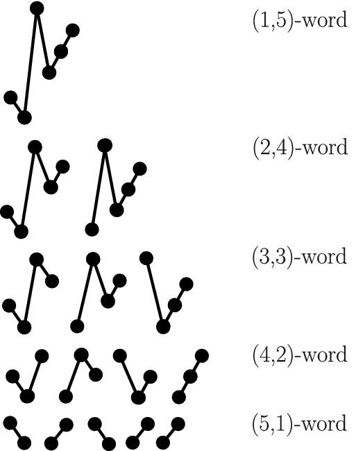
Figure 1 illustrates a segment (ω,T⁡(ω),…,T∘5​(ω))(\omega,T(\omega),\ldots,T^{\circ 5}(\omega)) of some orbit (a) and the corresponding (5,1)(5,1)-, (4,2)(4,2)-, (3,3)(3,3)-, (2,4)(2,4)- and (1,5)(1,5)-words (b).

Refer to caption

(a)

Refer to caption

(b)

Figure 1: Representation of the segment of the orbit (a) by (n,d)(n,d)-words (b)

Upon moving from (1,5)(1,5)- to (5,1)(5,1)-words one loses some information about the ordering of the iterates of TT. For example, the (3,3)(3,3)-word determines the relation

ω<T∘3​(ω),\omega<T^{\circ 3}(\omega),

but in the (4,2)(4,2)-word this relation is already lost. It either holds ω≥T∘3​(ω)\omega\geq T^{\circ 3}(\omega) or ω<T∘3​(ω)\omega<T^{\circ 3}(\omega).

On the other hand, one does not lose the relation

ω<T∘4​(ω)\omega<T^{\circ 4}(\omega)

when moving from the (2,4)(2,4)-word to the (3,3)(3,3)-word, although ω\omega and T∘4​(ω)T^{\circ 4}(\omega) are in different patterns of the (3,3)(3,3)-word. The reason for this is the existence of the intermediate iterate T∘3​(ω)T^{\circ 3}(\omega) with

ω<T∘3​(ω)<T∘4​(ω).\omega<T^{\circ 3}(\omega)<T^{\circ 4}(\omega).

More generally, if there is some intermediate iterate T∘l​(ω)T^{\circ l}(\omega) with ω<T∘l​(ω)<T∘d+1​(ω)\omega<T^{\circ l}(\omega)<T^{\circ d+1}(\omega) or T∘d+1​(ω)≤T∘l​(ω)≤ωT^{\circ d+1}(\omega)\leq T^{\circ l}(\omega)\leq\omega, the relation between ω\omega and T∘d+1​(ω)T^{\circ d+1}(\omega) is not lost upon moving from (1,d+1)(1,d+1)- to (2,d)(2,d)-words, and is lost otherwise. Therefore, the set Vd+1V_{d+1} (see (3)) consists of all ω\omega, for which the relation between ω\omega and T∘d+1​(ω)T^{\circ d+1}(\omega) is lost upon moving from (1,d+1)(1,d+1)- to (2,d)(2,d)-words. More precisely, the set Vd+1V_{d+1} is a union of the sets of the partition 𝒫⁡(d+1){\cal P}(d+1) that are proper subsets of some sets of the partition 𝒫​(d)2{\cal P}(d)_{2}.

Figure 2 illustrates ω,T∘2​(ω)∈V3\omega,T^{\circ 2}(\omega)\in V_{3} for our example.

Refer to caption

(a)

Refer to caption

(b)

Figure 2: ω∈V3\omega\in V_{3} (a), T∘2​(ω)∈V3T^{\circ 2}(\omega)\in V_{3} (b)

In the following section we compare the partitions 𝒫​(d)n{\cal P}(d)_{n} and 𝒫​(d+1)n−1{\cal P}(d+1)_{n-1} by means of the set Vd+1V_{d+1}.

3 The partitions 𝒫​(d+1)n−1{\cal P}(d+1)_{n-1} and 𝒫​(d)n{\cal P}(d)_{n}

Upon moving from (n−1,d+1)(n-1,d+1)- to (n,d)(n,d)-words, for i=0,1,…,n−2i=0,1,\ldots,n-2 the relation between T∘i​(ω)T^{\circ i}(\omega) and T∘d+i+1​(ω)T^{\circ d+i+1}(\omega) is lost iff T∘i​(ω)∈Vd+1T^{\circ i}(\omega)\in V_{d+1}. Therefore, if Vd+1≠∅V_{d+1}\neq\emptyset, then the partition 𝒫​(d+1)n−1{\cal P}(d+1)_{n-1} is properly finer than the partition 𝒫​(d)n{\cal P}(d)_{n}. The following is valid:

Proposition 5.

Given P∈𝒫​(d)nP\in{\cal P}(d)_{n}, let k=#{l∈{0,1,…,n−2}∣P⊂T−∘l(Vd+1)}k=\#\{l\in\{0,1,\ldots,n-2\}\mid P\subset T^{-\circ l}(V_{d+1})\}. Then there exist 2k2^{k} sets P1,P2,…,P2k∈𝒫​(d+1)n−1P_{1},P_{2},\ldots,P_{2^{k}}\in{\cal P}(d+1)_{n-1} with

P1∪P2∪…∪P2k=P.P_{1}\cup P_{2}\cup\ldots\cup P_{2^{k}}=P.
Proof.

Consider some P∈𝒫​(d)nP\in{\cal P}(d)_{n} and the corresponding (n,d)(n,d)-word. Since the (n,d)(n,d)-word determines the same dynamics for all ω∈P\omega\in P, for l=0,1,…,n−2l=0,1,\ldots,n-2 it holds either

P⊂T−∘l(Vd+1)P\subset T^{-\circ l}(V_{d+1}) (7)

or

P∩T−∘l(Vd+1)=∅.P\cap T^{-\circ l}(V_{d+1})=\emptyset. (8)

For each ll with (7) and all ω∈P\omega\in P, either T∘l​(ω)<T∘d+l+1​(ω)T^{\circ l}(\omega)<T^{\circ d+l+1}(\omega) or T∘d+l+1​(ω)≤T∘l​(ω)T^{\circ d+l+1}(\omega)\leq T^{\circ l}(\omega) providing a division of PP into two subset. We are done since there are exactly kk such divisions. ∎

Figure 3 illustrates Proposition 5.

Refer to caption
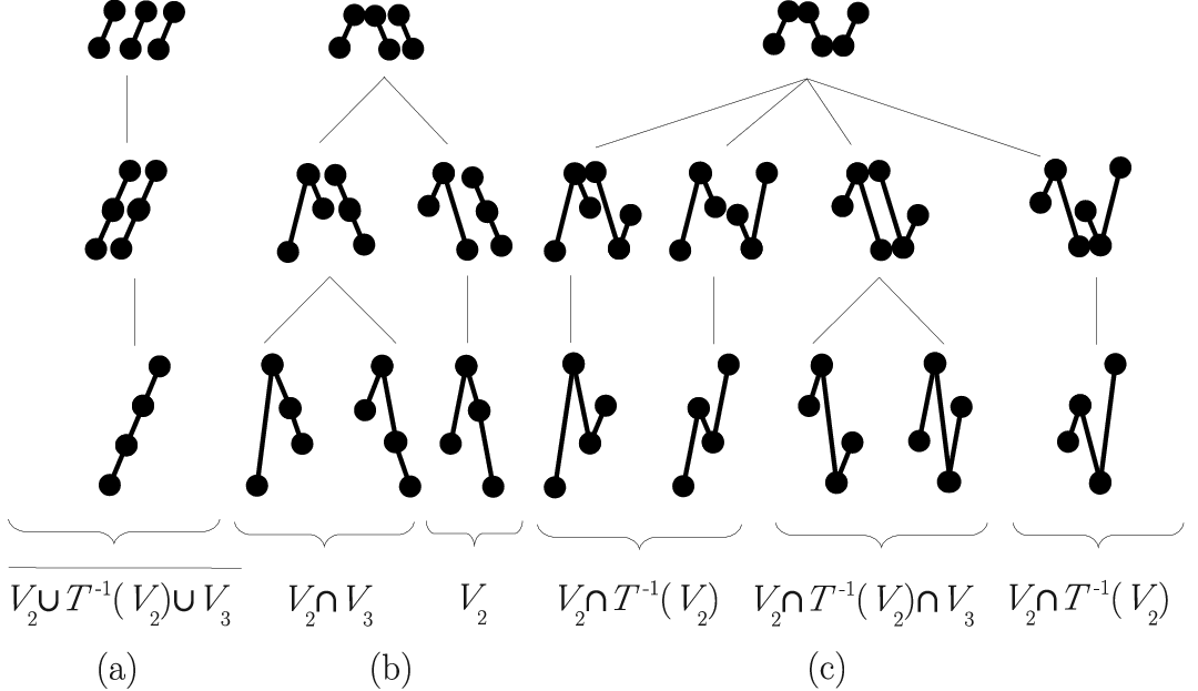
Figure 3: From (3,1)(3,1)- to (2,2)(2,2)-words. V2∪T−1​(V2)¯\overline{V_{2}\cup T^{-1}(V_{2})} in (a) stands for the complement of V2∪T−1​(V2)V_{2}\cup T^{-1}(V_{2})

For ω∉V2∪T−1​(V2)\omega\notin V_{2}\cup T^{-1}(V_{2}) the obtained (3,1)(3,1)-word is not divided and contains the same information about the ordering as 20=12^{0}=1 (2,2)(2,2)-word (a), for ω∈V2\omega\in V_{2} the (3,1)(3,1)-word is divided into 21=22^{1}=2 (2,2)(2,2)-words (b) and for ω∈V2∩T−1​(V2)\omega\in V_{2}\cap T^{-1}(V_{2}) the (3,1)(3,1)-word is divided into 22=42^{2}=4 (2,2)(2,2)-words (c).

Let k⁡(P)k(P) be determined as in Proposition 5 for each P∈𝒫​(d)nP\in{\cal P}(d)_{n}. Since for each PP it holds either (7) or (8), it follows

∑j=0n−2μ(T−∘j(Vd+1))=∑j=0n−2∑P∈𝒫​(d)nμ(T−∘j(Vd+1)∩P)=∑P∈𝒫​(d)nk(P)μ(P).\sum_{j=0}^{n-2}\mu(T^{-\circ j}(V_{d+1}))=\sum_{j=0}^{n-2}\sum_{P\in{\cal P}(d)_{n}}\mu(T^{-\circ j}(V_{d+1})\cap P)=\sum_{P\in{\cal P}(d)_{n}}k(P)\mu(P). (9)

Therefore, by Proposition 5 and (9) one obtains an upper bound for H⁡(𝒫​(d+1)n−1)−H⁡(𝒫​(d)n)H({\cal P}(d+1)_{n-1})-H({\cal P}(d)_{n}) in the following way:

H⁡(𝒫​(d+1)n−1)−H⁡(𝒫​(d)n)\displaystyle H({\cal P}(d+1)_{n-1})-H({\cal P}(d)_{n}) ≤∑P∈𝒫​(d)n(μ⁡(P)​ln⁡μ⁡(P)−2k⁡(P)​μ⁡(P)2k⁡(P)​ln⁡μ⁡(P)2k⁡(P))\displaystyle\leq\sum_{P\in{\cal P}(d)_{n}}\left(\mu(P)\ln\mu(P)-2^{k(P)}\frac{\mu(P)}{2^{k(P)}}\ln\frac{\mu(P)}{2^{k(P)}}\right)
=ln⁡2​∑P∈𝒫​(d)nk⁡(P)​μ​(P)\displaystyle=\ln 2\sum_{P\in{\cal P}(d)_{n}}k(P)\mu(P) =ln2∑j=0n−2μ(T−∘j(Vd+1))=ln2(n−1)μ(Vd+1).\displaystyle=\ln 2\sum_{j=0}^{n-2}\mu(T^{-\circ j}(V_{d+1}))=\ln 2(n-1)\mu(V_{d+1}). (10)

Inequality (10) provides the proof of Theorem 3.

4 The partitions 𝒫​(d)n{\cal P}(d)_{n} and 𝒫⁡(d+n−1){\cal P}(d+n-1)

Here we move from (1,d+n−1)(1,d+n-1)-words (i.e. ordinal patterns of order (d+n−1)(d+n-1)) to (n,d)(n,d)-words. At this point we cannot definitely say into how many (n,d)(n,d)-words a (1,d+n−1)(1,d+n-1)-word is divided in dependence on the sets Vd+1,…,Vd+n−1V_{d+1},\ldots,V_{d+n-1}.

Let us give an example. Figure 4 illustrates a (3,1)(3,1)-word with the same information as in the (1,3)(1,3)-word (a), other two (3,1)(3,1)-words are divided into three and five (1,3)(1,3)-words ((b) and (c), respectively).

Refer to caption
Figure 4: From (3,1)(3,1)- to (1,3)(1,3)-words. V2∪T−1​(V2)∪V3¯\overline{V_{2}\cup T^{-1}(V_{2})\cup V_{3}} in (a) stands for the complement of V2∪T−1​(V2)∪V3V_{2}\cup T^{-1}(V_{2})\cup V_{3}

One obtains an upper bound for H⁡(𝒫⁡(d+n−1))−H⁡(𝒫​(d)n)H({\cal P}(d+n-1))-H({\cal P}(d)_{n}) by successive application of (10):

H⁡(𝒫⁡(d+n−1))−H⁡(𝒫​(d)n)\displaystyle H({\cal P}(d+n-1))-H({\cal P}(d)_{n}) =∑i=1n−1(H⁡(𝒫​(d+n−i)i)−H⁡(𝒫​(d+n−i−1)i+1))\displaystyle=\sum_{i=1}^{n-1}(H({\cal P}(d+n-i)_{i})-H({\cal P}(d+n-i-1)_{i+1}))
≤ln⁡2​∑i=1n−1i​μ​(Vd+n−i)=ln⁡2​∑i=1n−1(n−i)​μ​(Vd+i).\displaystyle\leq\ln 2\sum_{i=1}^{n-1}i\,\mu(V_{d+n-i})=\ln 2\sum^{n-1}_{i=1}(n-i)\,\mu(V_{d+i}). (11)

Comparing (2) and (11) it is natural to ask how fast the measure of the set VdV_{d} decreases with increasing dd. This question is the subject of current research.

5 Proof of Theorem 2

In the following, we assume that TT is strong-mixing, however, some parts of the proof need only the weaker assumption of ergodicity, as we will indicate.

Lemma 6.

Let TT be ergodic. Given an interval A⊂ΩA\subset\Omega and d∈ℕ∖{1}d\in{\mathbb{N}}\setminus\{1\}, let V~d=V~d​(A)\widetilde{V}_{d}=\widetilde{V}_{d}(A) be the set of points ω∈A\omega\in A for which at least one of two following conditions holds:

T∘l​(ω)∉{a∈A|a<ω}​ for all ​l=1,…,d−1,T^{\circ l}(\omega)\notin\{a\in A\,|\,a<\omega\}\text{ for all }l=1,...,d-1, (12)
T∘l​(ω)∉{a∈A|a>ω}​ for all ​l=1,…,d−1.T^{\circ l}(\omega)\notin\{a\in A\,|\,a>\omega\}\text{ for all }l=1,...,d-1. (13)

Then for all ε>0\varepsilon>0 there exists some dε∈ℕd_{\varepsilon}\in{\mathbb{N}} such that μ⁡(V~d)<ε\mu(\widetilde{V}_{d})<\varepsilon for all d>dεd>d_{\varepsilon}.

Proof.

Let V~dL\widetilde{V}^{L}_{d} be a set of points ω\omega satisfying (12). Then it is sufficient to show μ⁡(V~dL)<ε2\mu(\widetilde{V}^{L}_{d})<\frac{\varepsilon}{2} for the corresponding dd since for points satisfying (13) the proof is completely resembling.

Consider a partition {Bi}i=1∞\{B_{i}\}_{i=1}^{\infty} of AA into intervals BiB_{i} with the following properties:

  1. (i)

    μ⁡(Bi)=μ⁡(A)2i\mu(B_{i})=\frac{\mu(A)}{2^{i}} for all i∈ℕi\in{\mathbb{N}},

  2. (ii)

    for all i<ji<j, and for all ω1∈Bi,ω2∈Bj\omega_{1}\in B_{i},\omega_{2}\in B_{j} it holds ω1>ω2\omega_{1}>\omega_{2}.

Since μ⁡({ω})=0\mu(\{\omega\})=0 for all ω∈Ω\omega\in\Omega, such partition always exists.

Define Di,d={ω∈Bi∣T∘l(ω)∉⋃j=i∞Bj for all l=1,…,d−1}D_{i,d}=\{\omega\in B_{i}\mid T^{\circ l}(\omega)\notin\bigcup_{j=i}^{\infty}B_{j}\text{ for all }l=1,...,d-1\}. It holds

⋃l=1d−1(Di,d∩T−∘l(⋃j=i∞Bj))=∅.\bigcup_{l=1}^{d-1}\left(D_{i,d}\cap T^{-\circ l}(\bigcup_{j=i}^{\infty}B_{j})\right)=\emptyset. (14)

For all d∈ℕd\in{\mathbb{N}}, (14) provides V~dL⊆⋃i=1∞Di,d\widetilde{V}^{L}_{d}\subseteq\bigcup_{i=1}^{\infty}D_{i,d} and, since Di,d⊆BiD_{i,d}\subseteq B_{i}, it holds

μ⁡(V~dL)\displaystyle\mu(\widetilde{V}^{L}_{d}) ≤μ⁡(⋃i=1∞Di,d)=∑i=1∞μ⁡(Di,d)≤∑i=1kμ⁡(Di,d)+∑i=k+1∞μ⁡(Bi)\displaystyle\leq\mu(\bigcup_{i=1}^{\infty}D_{i,d})=\sum_{i=1}^{\infty}\mu(D_{i,d})\leq\sum_{i=1}^{k}\mu(D_{i,d})+\sum_{i=k+1}^{\infty}\mu(B_{i})
≤∑i=1kμ⁡(Di,d)+∑i=k+1∞μ⁡(A)2i≤∑i=1kμ⁡(Di,d)+μ⁡(A)2k\displaystyle\leq\sum_{i=1}^{k}\mu(D_{i,d})+\sum_{i=k+1}^{\infty}\frac{\mu(A)}{2^{i}}\leq\sum_{i=1}^{k}\mu(D_{i,d})+\frac{\mu(A)}{2^{k}} (15)

for all k∈ℕk\in{\mathbb{N}}. On the other hand, by the ergodicity of TT (compare [10]) and by (14) we have

μ(⋂d=1∞Di,d)μ(⋃j=i∞Bj)=limm→∞1m∑l=1m−1μ(⋂d=1∞Di,d∩T−∘l(⋃j=i∞Bj))=0.\mu(\bigcap_{d=1}^{\infty}D_{i,d})\,\mu(\bigcup_{j=i}^{\infty}B_{j})=\lim_{m\to\infty}\frac{1}{m}\sum_{l=1}^{m-1}\mu\left(\bigcap_{d=1}^{\infty}D_{i,d}\cap T^{-\circ l}(\bigcup_{j=i}^{\infty}B_{j})\right)=0.

Therefore, μ⁡(⋃j=i∞Bj)>0\mu(\bigcup_{j=i}^{\infty}B_{j})>0 implies μ⁡(⋂d=1∞Di,d)=0\mu(\bigcap_{d=1}^{\infty}D_{i,d})=0 and, since Di,1⊇Di,2⊇…D_{i,1}\supseteq D_{i,2}\supseteq\ldots, it holds

limd→∞μ⁡(Di,d)=μ⁡(⋂d=1∞Di,d)=0\lim_{d\to\infty}\mu(D_{i,d})=\mu(\bigcap_{d=1}^{\infty}D_{i,d})=0

for all i∈ℕi\in{\mathbb{N}}.

Now let ε>0\varepsilon>0. Fix some k∈ℕk\in{\mathbb{N}} with k>log2⁡4εk>\log_{2}\frac{4}{\varepsilon} and dεd_{\varepsilon} with μ⁡(Di,d)<ε4​k\mu(D_{i,d})<\frac{\varepsilon}{4k} for all i=1,2,…,ki=1,2,\ldots,k and d>dεd>d_{\varepsilon}. Then, owing to (15), for d>dεd>d_{\varepsilon} it holds

μ⁡(V~dL)<k​ε4​k+ε4=ε2\mu(\widetilde{V}^{L}_{d})<k\,\frac{\varepsilon}{4k}+\frac{\varepsilon}{4}=\frac{\varepsilon}{2}

completing the proof. □\Box ∎

Now we are coming to the proof of Theorem 2. Given ε>0\varepsilon>0, let r>3εr>\frac{3}{\varepsilon} and let {Ai}i=1r\{A_{i}\}_{i=1}^{r} be a partition of Ω\Omega into intervals AiA_{i} with μ⁡(Ai)=1r\mu(A_{i})=\frac{1}{r}. Furthermore, fix some dε∈ℕd_{\varepsilon}\in{\mathbb{N}} with

μ(Ai∩T−∘d(Ai))≤μ2(Ai)+ε3​r=1r2+ε3​r\mu(A_{i}\cap T^{-\circ d}(A_{i}))\leq\mu^{2}(A_{i})+\frac{\varepsilon}{3r}=\frac{1}{r^{2}}+\frac{\varepsilon}{3r} (16)

and

μ⁡(V~d)≤ε3​r\mu(\widetilde{V}_{d})\leq\frac{\varepsilon}{3r} (17)

for all i=1,2,…,ri=1,2,\ldots,r and all d>dεd>d_{\varepsilon}, which is possible by the strong-mixing of TT and by Lemma 6, respectively.

For ω∈Vd∩Ai\omega\in V_{d}\cap A_{i} it is impossible that both T∘d​(ω)∉AiT^{\circ d}(\omega)\not\in A_{i} and ω∉V~d​(Ai)\omega\not\in\widetilde{V}_{d}(A_{i}), implying

Vd=⋃i=1r(Vd∩Ai)\displaystyle V_{d}=\bigcup_{i=1}^{r}\,(V_{d}\cap A_{i}) ⊂\displaystyle\subset ⋃i=1r((Ai∩T−∘d(Ai))∪V~d(Ai))\displaystyle\bigcup_{i=1}^{r}\,((A_{i}\cap T^{-\circ d}(A_{i}))\cup\widetilde{V}_{d}(A_{i}))
=\displaystyle= ⋃i=1r(Ai∩T−∘d(Ai))∪⋃i=1rV~d(Ai).\displaystyle\bigcup_{i=1}^{r}\,(A_{i}\cap T^{-\circ d}(A_{i}))\cup\bigcup_{i=1}^{r}\,\widetilde{V}_{d}(A_{i}).

From this, (16), and (17), one obtains

μ⁡(Vd)\displaystyle\mu(V_{d}) ≤\displaystyle\leq ∑i=1rμ(Ai∩T−∘d(Ai))+∑i=1rμ(V~d(Ai))\displaystyle\sum_{i=1}^{r}\,\mu(A_{i}\cap T^{-\circ d}(A_{i}))+\sum_{i=1}^{r}\,\mu(\widetilde{V}_{d}(A_{i}))
≤\displaystyle\leq r⁡(1r2+ε3​r)+ε3<ε.\displaystyle r\left(\frac{1}{r^{2}}+\frac{\varepsilon}{3r}\right)+\frac{\varepsilon}{3}<\varepsilon.
Remark.

The technical assumption that μ⁡({ω})=0\mu(\{\omega\})=0 for all ω∈Ω\omega\in\Omega is rather weak. In the ergodic (resp. strong-mixing) case, μ⁡({ω})>0\mu(\{\omega\})>0 would imply that ω\omega is a periodic (resp. fixed) point and that μ\mu is concentrated on the orbit of ω\omega (resp. on ω\omega).

This work was supported by the Graduate School for Computing in Medicine and Life Sciences funded by Germany’s Excellence Initiative [DFG GSC 235/1].

References

  • [1] C. Bandt, B. Pompe, Phys. Rev. Lett. 88, 174102 (2002)
  • [2] C. Bandt, G. Keller, B. Pompe, Nonlinearity 15, 1595 (2002)
  • [3] K. Keller and M. Sinn, Nonlinearity 22, 2417 (2009)
  • [4] K. Keller and M. Sinn, Physica D 239, 997 (2010)
  • [5] K. Keller, Discrete and Continuous Dynamical Systems A 32, 891 (2011)
  • [6] J.M. Amigó, M.B. Kennel, L. Kocarev, Physica D 210, 77 (2005)
  • [7] J.M. Amigó, Physica D 241, 789 (2012)
  • [8] J.M. Amigó, Permutation Complexity in Dynamical Systems, (Springer-Verlag, Berlin-Heidelberg 2010)
  • [9] K. Keller, A.M. Unakafov, V.A. Unakafova, Physica D 241, 1477 (2012)
  • [10] P. Walters, An Introduction to Ergodic Theory, (Springer-Verlag, New York 2000)