跳到论文正文
W Papers独立论文阅读器 arXiv:1503.02101 论文正文 计算阅读时间 · 0%
引用这篇论文根据当前论文元数据生成,正式投稿前建议核对。


License: arXiv.org perpetual non-exclusive license
arXiv:1503.02101v1 [cs.LG] 06 Mar 2015

Escaping From Saddle Points –
Online Stochastic Gradient for Tensor Decomposition

Rong Ge ††thanks: Microsoft Research New England, rongge@microsoft.com    Furong Huang ††thanks: University of California Irvine, Department of Electrical Engineering and Computer Science, furongh@uci.edu    Chi Jin ††thanks: University of California Berkeley, Department of Electrical Engineering and Computer Science, chijin@cs.berkeley.edu    Yang Yuan ††thanks: Cornell University, Computer Science Department, yangyuan@cs.cornell.edu
Abstract

We analyze stochastic gradient descent for optimizing non-convex functions. In many cases for non-convex functions the goal is to find a reasonable local minimum, and the main concern is that gradient updates are trapped in saddle points. In this paper we identify strict saddle property for non-convex problem that allows for efficient optimization. Using this property we show that stochastic gradient descent converges to a local minimum in a polynomial number of iterations. To the best of our knowledge this is the first work that gives global convergence guarantees for stochastic gradient descent on non-convex functions with exponentially many local minima and saddle points.

Our analysis can be applied to orthogonal tensor decomposition, which is widely used in learning a rich class of latent variable models. We propose a new optimization formulation for the tensor decomposition problem that has strict saddle property. As a result we get the first online algorithm for orthogonal tensor decomposition with global convergence guarantee.

1 Introduction

Stochastic gradient descent is one of the basic algorithms in optimization. It is often used to solve the following stochastic optimization problem

w=arg⁡minw∈ℝd⁡f⁡(w), where ​f​(w)=𝔼x∼𝒟​[ϕ⁡(w,x)]w=\arg\min_{w\in\mathbb{R}^{d}}f(w),\textrm{~where~}f(w)=\mathbb{E}_{x\sim\mathcal{D}}[\phi(w,x)] (1)

Here xx is a data point that comes from some unknown distribution 𝒟\mathcal{D}, and ϕ\phi is a loss function that is defined for a pair (x,w)(x,w). We hope to minimize the expected loss 𝔼⁡[ϕ⁡(w,x)]\mathbb{E}[\phi(w,x)].

When the function f⁡(w)f(w) is convex, convergence of stochastic gradient descent is well-understood (Rakhlin et al.,, 2012; Shalev-Shwartz et al.,, 2009). However, stochastic gradient descent is not only limited to convex functions. Especially, in the context of neural networks, stochastic gradient descent is known as the “backpropagation” algorithm (Rumelhart et al.,, 1988), and has been the main algorithm that underlies the success of deep learning (Bengio,, 2009). However, the guarantees in the convex setting does not transfer to the non-convex settings.

Optimizing a non-convex function is NP-hard in general. The difficulty comes from two aspects. First, a non-convex function may have many local minima, and it might be hard to find the best one (global minimum) among them. Second, even finding a local minimum might be hard as there can be many saddle points which have 00-gradient but are not local minima11 1 See Section 3 for definition of saddle points.. In the most general case, there is no known algorithm that guarantees to find a local minimum in polynomial number of steps. The discrete analog (finding local minimum in domains like {0,1}n\{0,1\}^{n}) has been studied in complexity theory and is PLS-complete (Johnson et al.,, 1988).

In many cases, especially in those related to deep neural networks (Dauphin et al.,, 2014)
(Choromanska et al.,, 2014), the main bottleneck in optimization is not due to local minima, but the existence of many saddle points. Gradient based algorithms are in particular susceptible to saddle point problems as they only rely on the gradient information. The saddle point problem is alleviated for second-order methods that also rely on the Hessian information (Dauphin et al.,, 2014).

However, using Hessian information usually increases the memory requirement and computation time per iteration. As a result many applications still use stochastic gradient and empirically get reasonable results. In this paper we investigate why stochastic gradient methods can be effective even in presence of saddle point, in particular we answer the following question:

Question: Given a non-convex function ff with many saddle points, what properties of ff will guarantee stochastic gradient descent to converge to a local minimum efficiently?

We identify a property of non-convex functions which we call strict saddle. Intuitively, this property guarantees local progress if we have access to the Hessian information. Surprisingly we show with only first order (gradient) information, stochastic gradient can escape the saddle points efficiently. We give a framework for analyzing stochastic gradient in both unconstrained and equality-constrained case using this property.

We apply our framework to orthogonal tensor decomposition, which is a core problem in learning many latent variable models (see discussion in 2.2). The tensor decomposition problem is inherently susceptible to the saddle point issues, as the problem asks to find dd different components and any permutation of the true components yields a valid solution. Such symmetry creates exponentially many local minima and saddle points in the optimization problem. Using our new analysis of stochastic gradient, we give the first online algorithm for orthogonal tensor decomposition with global convergence guarantee. This is a key step towards making tensor decomposition algorithms more scalable.

1.1 Summary of Results

Strict saddle functions

Given a function f⁡(w)f(w) that is twice differentiable, we call ww a stationary point if ∇f​(w)=0\nabla f(w)=0. A stationary point can either be a local minimum, a local maximum or a saddle point. We identify an interesting class of non-convex functions which we call strict saddle. For these functions the Hessian of every saddle point has a negative eigenvalue. In particular, this means that local second-order algorithms which are similar to the ones in (Dauphin et al.,, 2014) can always make some progress.

It may seem counter-intuitive why stochastic gradient can work in these cases: in particular if we run the basic gradient descent starting from a stationary point then it will not move. However, we show that the saddle points are not stable and that the randomness in stochastic gradient helps the algorithm to escape from the saddle points.

Theorem 1 (informal).

Suppose f⁡(w)f(w) is strict saddle (see Definition 5), Noisy Gradient Descent (Algorithm 1) outputs a point that is close to a local minimum in polynomial number of steps.

Online tensor decomposition

Requiring all saddle points to have a negative eigenvalue may seem strong, but it already allows non-trivial applications to natural non-convex optimization problems. As an example, we consider the orthogonal tensor decomposition problem. This problem is the key step in spectral learning for many latent variable models (see more discussions in Section 2.2).

We design a new objective function for tensor decomposition that is strict saddle.

Theorem 2.

Given random samples XX such that T=𝔼⁡[g⁡(X)]∈ℝd4T=\mathbb{E}[g(X)]\in\mathbb{R}^{d^{4}} is an orthogonal 44-th order tensor (see Section 2.2), there is an objective function f⁡(w)=𝔼⁡[ϕ⁡(w,X)]f(w)=\mathbb{E}[\phi(w,X)] w∈ℝd×dw\in\mathbb{R}^{d\times d} such that every local minimum of f⁡(w)f(w) corresponds to a valid decomposition of TT. Further, function ff is strict saddle.

Combining this new objective with our framework for analyzing stochastic gradient in non-convex setting, we get the first online algorithm for orthogonal tensor decomposition with global convergence guarantee.

1.2 Related Works

Relaxed notions of convexity

In optimization theory and economics, there are extensive works on understanding functions that behave similarly to convex functions (and in particular can be optimized efficiently). Such notions involve pseudo-convexity (Mangasarian,, 1965), quasi-convexity 
(Kiwiel,, 2001), invexity(Hanson,, 1999) and their variants. More recently there are also works that consider classes that admit more efficient optimization procedures like RSC (restricted strong convexity) (Agarwal et al.,, 2010). Although these classes involve functions that are non-convex, the function (or at least the function restricted to the region of analysis) still has a unique stationary point that is the desired local/global minimum. Therefore these works cannot be used to prove global convergence for problems like tensor decomposition, where by symmetry of the problem there are multiple local minima and saddle points.

Second-order algorithms

The most popular second-order method is the Newton’s method. Although Newton’s method converges fast near a local minimum, its global convergence properties are less understood in the more general case. For non-convex functions, (Frieze et al.,, 1996) gave a concrete example where second-order method converges to the desired local minimum in polynomial number of steps (interestingly the function of interest is trying to find one component in a 44-th order orthogonal tensor, which is a simpler case of our application). As Newton’s method often converges also to saddle points, to avoid this behavior, different trusted-region algorithms are applied (Dauphin et al.,, 2014).

Stochastic gradient and symmetry

The tensor decomposition problem we consider in this paper has the following symmetry: the solution is a set of dd vectors v1,…,vdv_{1},...,v_{d}. If (v1,v2,…,vd)(v_{1},v_{2},...,v_{d}) is a solution, then for any permutation π\pi and any sign flips κ∈{±1}d\kappa\in\{\pm 1\}^{d}, (..,κivπ⁡(i),…)(..,\kappa_{i}v_{\pi(i)},...) is also a valid solution. In general, symmetry is known to generate saddle points, and variants of gradient descent often perform reasonably in these cases (see (Saad and Solla,, 1995), (Rattray et al.,, 1998), (Inoue et al.,, 2003)). The settings in these work are different from ours, and none of them give bounds on number of steps required for convergence.

There are many other problems that have the same symmetric structure as the tensor decomposition problem, including the sparse coding problem (Olshausen and Field,, 1997) and many deep learning applications (Bengio,, 2009). In these problems the goal is to learn multiple “features” where the solution is invariant under permutation. Note that there are many recent papers on iterative/gradient based algorithms for problems related to matrix factorization (Jain et al.,, 2013; Saxe et al.,, 2013). These problems often have very different symmetry, as if Y=A​XY=AX then for any invertible matrix RR we know Y=(A​R)​(R−1​X)Y=(AR)(R^{-1}X). In this case all the equivalent solutions are in a connected low dimensional manifold and there need not be saddle points between them.

2 Preliminaries

Notation

Throughout the paper we use [d][d] to denote set {1,2,…,d}\{1,2,...,d\}. We use ∥⋅∥\|\cdot\| to denote the ℓ2\ell_{2} norm of vectors and spectral norm of matrices. For a matrix we use λm​i​n\lambda_{min} to denote its smallest eigenvalue. For a function f:ℝd→ℝf:\mathbb{R}^{d}\to\mathbb{R}, ∇f\nabla f and ∇2f\nabla^{2}f denote its gradient vector and Hessian matrix.

2.1 Stochastic Gradient Descent

The stochastic gradient aims to solve the stochastic optimization problem (1), which we restate here:

w=arg⁡minw∈ℝd⁡f⁡(w), where ​f​(w)=𝔼x∼𝒟​[ϕ⁡(w,x)].w=\arg\min_{w\in\mathbb{R}^{d}}f(w),\textrm{~where~}f(w)=\mathbb{E}_{x\sim\mathcal{D}}[\phi(w,x)].

Recall ϕ⁡(w,x)\phi(w,x) denotes the loss function evaluated for sample xx at point ww. The algorithm follows a stochastic gradient

wt+1=wt−η​∇wtϕ​(wt,xt),w_{t+1}=w_{t}-\eta\nabla_{w_{t}}\phi(w_{t},x_{t}), (2)

where xtx_{t} is a random sample drawn from distribution 𝒟\mathcal{D} and η\eta is the learning rate.

In the more general setting, stochastic gradient descent can be viewed as optimizing an arbitrary function f⁡(w)f(w) given a stochastic gradient oracle.

Definition 3.

For a function f⁡(w):ℝd→ℝf(w):\mathbb{R}^{d}\to\mathbb{R}, a function S​G​(w)SG(w) that maps a variable to a random vector in ℝd\mathbb{R}^{d} is a stochastic gradient oracle if 𝔼​[S​G​(w)]=∇f​(w)\mathbb{E}[SG(w)]=\nabla f(w) and ‖S​G​(w)−∇f​(w)‖≤Q\|SG(w)-\nabla f(w)\|\leq Q.

In this case the update step of the algorithm becomes wt+1=wt−η​S​G​(wt)w_{t+1}=w_{t}-\eta SG(w_{t}).

Smoothness and Strong Convexity

Traditional analysis for stochastic gradient often assumes the function is smooth and strongly convex. A function is β\beta-smooth if for any two points w1,w2w_{1},w_{2},

‖∇f​(w1)−∇f​(w2)‖≤β​‖w1−w2‖.\|\nabla f(w_{1})-\nabla f(w_{2})\|\leq\beta\|w_{1}-w_{2}\|. (3)

When ff is twice differentiable this is equivalent to assuming that the spectral norm of the Hessian matrix is bounded by β\beta. We say a function is α\alpha-strongly convex if the Hessian at any point has smallest eigenvalue at least α\alpha (λm​i​n​(∇2f​(w))≥α\lambda_{min}(\nabla^{2}f(w))\geq\alpha).

Using these two properties, previous work (Rakhlin et al.,, 2012) shows that stochastic gradient converges at a rate of 1/t1/t. In this paper we consider non-convex functions, which can still be β\beta-smooth but cannot be strongly convex.

Smoothness of Hessians

We also require the Hessian of the function ff to be smooth. We say a function f⁡(w)f(w) has ρ\rho-Lipschitz Hessian if for any two points w1,w2w_{1},w_{2} we have

‖∇2f​(w1)−∇2f​(w2)‖≤ρ​‖w1−w2‖.\|\nabla^{2}f(w_{1})-\nabla^{2}f(w_{2})\|\leq\rho\|w_{1}-w_{2}\|. (4)

This is a third order condition that is true if the third order derivative exists and is bounded.

2.2 Tensors decomposition

A pp-th order tensor is a pp-dimensional array. In this paper we will mostly consider 44-th order tensors. If T∈ℝd4T\in\mathbb{R}^{d^{4}} is a 44-th order tensor, we use Ti1,i2,i3,i4​(i1,…,i4∈[d])T_{i_{1},i_{2},i_{3},i_{4}}(i_{1},...,i_{4}\in[d]) to denote its (i1,i2,i3,i4)(i_{1},i_{2},i_{3},i_{4})-th entry.

Tensors can be constructed from tensor products. We use (u⊗v)(u\otimes v) to denote a 22nd order tensor where (u⊗v)i,j=ui​vj(u\otimes v)_{i,j}=u_{i}v_{j}. This generalizes to higher order and we use u⊗4u^{\otimes 4} to denote the 44-th order tensor

[u⊗4]i1,i2,i3,i4=ui1​ui2​ui3​ui4.[u^{\otimes 4}]_{i_{1},i_{2},i_{3},i_{4}}=u_{i_{1}}u_{i_{2}}u_{i_{3}}u_{i_{4}}.

We say a 44-th order tensor T∈ℝd4T\in\mathbb{R}^{d^{4}} has an orthogonal decomposition if it can be written as

T=∑i=1dai⊗4,T=\sum_{i=1}^{d}a_{i}^{\otimes 4}, (5)

where aia_{i}’s are orthonormal vectors that satisfy ‖ai‖=1\|a_{i}\|=1 and aiT​aj=0a_{i}^{T}a_{j}=0 for i≠ji\neq j. We call the vectors aia_{i}’s the components of this decomposition. Such a decomposition is unique up to permutation of aia_{i}’s and sign-flips.

A tensor also defines a multilinear form (just as a matrix defines a bilinear form), for a pp-th order tensor T∈ℝdpT\in\mathbb{R}^{d^{p}} and matrices Mi∈ℝd×ni​i∈[p]M_{i}\in\mathbb{R}^{d\times n_{i}}i\in[p], we define

[T⁡(M1,M2,…,Mp)]i1,i2,…,ip=∑j1,j2,…,jp∈[d]Tj1,j2,…,jp​∏t∈[p]Mt​[it,jt].[T(M_{1},M_{2},...,M_{p})]_{i_{1},i_{2},...,i_{p}}=\sum_{j_{1},j_{2},...,j_{p}\in[d]}T_{j_{1},j_{2},...,j_{p}}\prod_{t\in[p]}M_{t}[i_{t},j_{t}].

That is, the result of the multilinear form T⁡(M1,M2,…,Mp)T(M_{1},M_{2},...,M_{p}) is another tensor in ℝn1×n2×⋯×np\mathbb{R}^{n_{1}\times n_{2}\times\cdots\times n_{p}}. We will most often use vectors or identity matrices in the multilinear form. In particular, for a 44-th order tensor T∈ℝd4T\in\mathbb{R}^{d^{4}} we know T⁡(I,u,u,u)T(I,u,u,u) is a vector and T⁡(I,I,u,u)T(I,I,u,u) is a matrix. In particular, if TT has the orthogonal decomposition in (5), we know T⁡(I,u,u,u)=∑i=1d(uT​ai)3​aiT(I,u,u,u)=\sum_{i=1}^{d}(u^{T}a_{i})^{3}a_{i} and T⁡(I,I,u,u)=∑i=1d(uT​ai)2​ai​aiTT(I,I,u,u)=\sum_{i=1}^{d}(u^{T}a_{i})^{2}a_{i}a_{i}^{T}.

Given a tensor TT with an orthogonal decomposition, the orthogonal tensor decomposition problem asks to find the individual components a1,…,ada_{1},...,a_{d}. This is a central problem in learning many latent variable models, including Hidden Markov Model, multi-view models, topic models, mixture of Gaussians and Independent Component Analysis (ICA). See the discussion and citations in Anandkumar et al., (2014). Orthogonal tensor decomposition problem can be solved by many algorithms even when the input is a noisy estimation T~≈T\tilde{T}\approx T  (Harshman,, 1970; Kolda,, 2001; Anandkumar et al.,, 2014). In practice this approach has been successfully applied to ICA (Comon,, 2002), topic models (Zou et al.,, 2013) and community detection (Huang et al.,, 2013).

3 Stochastic gradient descent for strict saddle function

In this section we discuss the properties of saddle points, and show if all the saddle points are well-behaved then stochastic gradient descent finds a local minimum for a non-convex function in polynomial time.

3.1 Strict saddle property

For a twice differentiable function f⁡(w)f(w), we call the points stationary points if their gradients are equal to 00. Stationary points could be local minima, local maxima or saddle points. By local optimality conditions (Wright and Nocedal,, 1999), in many cases we can tell what type a point ww is by looking at its Hessian: if ∇2f​(w)\nabla^{2}f(w) is positive definite then ww is a local minimum; if ∇2f​(w)\nabla^{2}f(w) is negative definite then ww is a local maximum; if ∇2f​(w)\nabla^{2}f(w) has both positive and negative eigenvalues then ww is a saddle point. These criteria do not cover all the cases as there could be degenerate scenarios: ∇2f​(w)\nabla^{2}f(w) can be positive semidefinite with an eigenvalue equal to 0, in which case the point could be a local minimum or a saddle point.

If a function does not have these degenerate cases, then we say the function is strict saddle:

Definition 4.

A twice differentiable function f⁡(w)f(w) is strict saddle, if all its local minima have ∇2f​(w)≻0\nabla^{2}f(w)\succ 0 and all its other stationary points satisfy λm​i​n​(∇2f​(w))<0\lambda_{min}(\nabla^{2}f(w))<0.

Intuitively, if we are not at a stationary point, then we can always follow the gradient and reduce the value of the function. If we are at a saddle point, we need to consider a second order Taylor expansion:

f⁡(w+Δ​w)≈w+(Δ​w)T​∇2f​(w)​(Δ​w)+O⁡(‖Δ​w‖3).f(w+\Delta w)\approx w+(\Delta w)^{T}\nabla^{2}f(w)(\Delta w)+O(\|\Delta w\|^{3}).

Since the strict saddle property guarantees ∇2f​(w)\nabla^{2}f(w) to have a negative eigenvalue, there is always a point that is near ww and has strictly smaller function value. It is possible to make local improvements as long as we have access to second order information. However it is not clear whether the more efficient stochastic gradient updates can work in this setting.

To make sure the local improvements are significant, we use a robust version of the strict saddle property:

Definition 5.

A twice differentiable function f⁡(w)f(w) is (α,γ,ϵ,δ)(\alpha,\gamma,\epsilon,\delta)-strict saddle, if for any point ww at least one of the following is true

  1. 1.

    ‖∇f​(w)‖≥ϵ\|\nabla f(w)\|\geq\epsilon.

  2. 2.

    λm​i​n​(∇2f​(w))≤−γ\lambda_{min}(\nabla^{2}f(w))\leq-\gamma.

  3. 3.

    There is a local minimum w⋆w^{\star} such that ‖w−w⋆‖≤δ\|w-w^{\star}\|\leq\delta, and the function f⁡(w′)f(w^{\prime}) restricted to 2​δ2\delta neighborhood of w⋆w^{\star} (‖w′−w⋆‖≤2​δ\|w^{\prime}-w^{\star}\|\leq 2\delta) is α\alpha-strongly convex.

Intuitively, this condition says for any point whose gradient is small, it is either close to a robust local minimum, or is a saddle point (or local maximum) with a significant negative eigenvalue.

Algorithm 1 Noisy Stochastic Gradient
0:  Stochastic gradient oracle S​G​(w)SG(w), initial point w0w_{0}, desired accuracy κ\kappa.
0:  wtw_{t} that is close to some local minimum w⋆w^{\star}.
1:  Choose η=min⁡{O~​(κ2/log⁡(1/κ)),ηmax}\eta=\min\{\tilde{O}(\kappa^{2}/\log(1/\kappa)),\eta_{\max}\}, T=O~​(1/η2)T=\tilde{O}(1/\eta^{2})
2:  for t=0t=0 to T−1T-1 do
3:   Sample noise nn uniformly from unit sphere.
4:   wt+1←wt−η⁡(S​G​(w)+n)w_{t+1}\leftarrow w_{t}-\eta(SG(w)+n)

We purpose a simple variant of stochastic gradient algorithm, where the only difference to the traditional algorithm is we add an extra noise term to the updates. The main benefit of this additional noise is that we can guarantee there is noise in every direction, which allows the algorithm to effectively explore the local neighborhood around saddle points. If the noise from stochastic gradient oracle already has nonnegligible variance in every direction, our analysis also applies without adding additional noise. We show noise can help the algorithm escape from saddle points and optimize strict saddle functions.

Theorem 6 (Main Theorem).

Suppose a function f⁡(w):ℝd→ℝf(w):\mathbb{R}^{d}\to\mathbb{R} that is (α,γ,ϵ,δ)(\alpha,\gamma,\epsilon,\delta)-strict saddle, and has a stochastic gradient oracle with radius at most QQ. Further, suppose the function is bounded by |f⁡(w)|≤B|f(w)|\leq B, is β\beta-smooth and has ρ\rho-Lipschitz Hessian. Then there exists a threshold ηmax=Θ~​(1)\eta_{\max}=\tilde{\Theta}(1), so that for any ζ>0\zeta>0, and for any η≤ηmax/max⁡{1,log⁡(1/ζ)}\eta\leq\eta_{\max}/\max\{1,\log(1/\zeta)\}, with probability at least 1−ζ1-\zeta in t=O~​(η−2​log⁡(1/ζ))t=\tilde{O}(\eta^{-2}\log(1/\zeta)) iterations, Algorithm 1 (Noisy Gradient Descent) outputs a point wtw_{t} that is O~​(η​log⁡(1/η​ζ))\tilde{O}(\sqrt{\eta\log(1/\eta\zeta)})-close to some local minimum w⋆w^{\star}.

Here (and throughout the rest of the paper) O~​(⋅)\tilde{O}(\cdot) (Ω~,Θ~\tilde{\Omega},\tilde{\Theta}) hides the factor that is polynomially dependent on all other parameters (including QQ, 1/α1/\alpha, 1/γ1/\gamma, 1/ϵ1/\epsilon, 1/δ1/\delta, BB, β\beta, ρ\rho, and dd), but independent of η\eta and ζ\zeta. So it focuses on the dependency on η\eta and ζ\zeta. Our proof technique can give explicit dependencies on these parameters however we hide these dependencies for simplicity of presentation.

Remark (Decreasing learning rate).

Often analysis of stochastic gradient descent uses decreasing learning rates and the algorithm converges to a local (or global) minimum. Since the function is strongly convex in the small region close to local minimum, we can use Theorem 6 to first find a point that is close to a local minimum, and then apply standard analysis of SGD in the strongly convex case (where we decrease the learning rate by 1/t1/t and get 1/t1/\sqrt{t} convergence in ‖w−w⋆‖\|w-w^{\star}\|).

In the next part we sketch the proof of the main theorem. Details are deferred to Appendix A.

3.2 Proof sketch

In order to prove Theorem 6, we analyze the three cases in Definition 5. When the gradient is large, we show the function value decreases in one step (see Lemma 7); when the point is close to a local minimum, we show with high probability it cannot escape in the next polynomial number of iterations (see Lemma 8).

Lemma 7 (Gradient).

Under the assumptions of Theorem 6, for any point with ‖∇f​(wt)‖≥C​η\|\nabla f(w_{t})\|\geq C\sqrt{\eta} (where C=Θ~​(1)C=\tilde{\Theta}(1)) and C​η≤ϵC\sqrt{\eta}\leq\epsilon, after one iteration we have 𝔼⁡[f⁡(wt+1)]≤f⁡(wt)−Ω~​(η2)\mathbb{E}[f(w_{t+1})]\leq f(w_{t})-\tilde{\Omega}(\eta^{2}).

The proof of this lemma is a simple application of the smoothness property.

Lemma 8 (Local minimum).

Under the assumptions of Theorem 6, for any point wtw_{t} that is O~​(η)<δ\tilde{O}(\sqrt{\eta})<\delta close to local minimum w⋆w^{\star}, in O~​(η−2​log⁡(1/ζ))\tilde{O}(\eta^{-2}\log(1/\zeta)) number of steps all future wt+iw_{t+i}’s are O~​(η​log⁡(1/η​ζ))\tilde{O}(\sqrt{\eta\log(1/\eta\zeta)})-close with probability at least 1−ζ/21-\zeta/2.

The proof of this lemma is similar to the standard analysis (Rakhlin et al.,, 2012) of stochastic gradient descent in the smooth and strongly convex setting, except we only have local strongly convexity. The proof appears in Appendix A.

The hardest case is when the point is “close” to a saddle point: it has gradient smaller than ϵ\epsilon and smallest eigenvalue of the Hessian bounded by −γ-\gamma. In this case we show the noise in our algorithm helps the algorithm to escape:

Lemma 9 (Saddle point).

Under the assumptions of Theorem 6, for any point wtw_{t} where ‖∇f​(wt)‖≤C​η\|\nabla f(w_{t})\|\leq C\sqrt{\eta} (for the same CC as in Lemma 7), and λmin​(∇2f​(wt))≤−γ\lambda_{\min}(\nabla^{2}f(w_{t}))\leq-\gamma, there is a number of steps TT that depends on wtw_{t} such that 𝔼⁡[f⁡(wt+T)]≤f⁡(wt)−Ω~​(η)\mathbb{E}[f(w_{t+T})]\leq f(w_{t})-\tilde{\Omega}(\eta). The number of steps TT has a fixed upper bound Tm​a​xT_{max} that is independent of wtw_{t} where T≤Tm​a​x=O~​(1/η)T\leq T_{max}=\tilde{O}(1/\eta).

Intuitively, at point wtw_{t} there is a good direction that is hiding in the Hessian. The hope of the algorithm is that the additional (or inherent) noise in the update step makes a small step towards the correct direction, and then the gradient information will reinforce this small perturbation and the future updates will “slide” down the correct direction.

To make this more formal, we consider a coupled sequence of updates w~\tilde{w} such that the function to minimize is just the local second order approximation

f~(w)=f(wt)+∇f(wt)T(w−wt)+12(w−wt)T∇2f(wt)(w−wt).\tilde{f}(w)=f(w_{t})+\nabla f(w_{t})^{T}(w-w_{t})+\frac{1}{2}(w-w_{t})^{T}\nabla^{2}f(w_{t})(w-w_{t}).

The dynamics of stochastic gradient descent for this quadratic function is easy to analyze as w~t+i\tilde{w}_{t+i} can be calculated analytically. Indeed, we show the expectation of f~​(w~)\tilde{f}(\tilde{w}) will decrease. We then use the smoothness of the function to show that as long as the points did not go very far from wtw_{t}, the two update sequences w~\tilde{w} and ww will remain close to each other, and thus f~​(w~t+i)≈f⁡(wt+i)\tilde{f}(\tilde{w}_{t+i})\approx f(w_{t+i}). Finally we prove the future wt+iw_{t+i}’s (in the next TT steps) will remain close to wtw_{t} with high probability by Martingale bounds. The detailed proof appears in Appendix A.

With these three lemmas it is easy to prove the main theorem. Intuitively, as long as there is a small probability of being O~​(η)\tilde{O}(\sqrt{\eta})-close to a local minimum, we can always apply Lemma 7 or Lemma 9 to make the expected function value decrease by Ω~​(η)\tilde{\Omega}(\eta) in at most O~​(1/η)\tilde{O}(1/\eta) iterations, this cannot go on for more than O~​(1/η2)\tilde{O}(1/\eta^{2}) iterations because in that case the expected function value will decrease by more than 2​B2B, but max⁡f⁡(x)−min⁡f⁡(x)≤2​B\max f(x)-\min f(x)\leq 2B by our assumption. Therefore in O~​(1/η2)\tilde{O}(1/\eta^{2}) steps with at least constant probability wtw_{t} will become O~​(η)\tilde{O}(\sqrt{\eta})-close to a local minimum. By Lemma 8 we know once it is close it will almost always stay close, so we can repeat this log⁡(1/ζ)\log(1/\zeta) times to get the high probability result. More details appear in Appendix A.

3.3 Constrained Problems

In many cases, the problem we are facing are constrained optimization problems. In this part we briefly describe how to adapt the analysis to problems with equality constraints (which suffices for the tensor application). Dealing with general inequality constraint is left as future work.

For a constrained optimization problem:

minw∈ℝdf⁡(w)\displaystyle\min_{w\in\mathbb{R}^{d}}\quad\quad f(w) (6)
s.t.ci​(w)=0,i∈[m]\displaystyle\text{s.t.}\quad\quad c_{i}(w)=0,\quad\quad i\in[m]

in general we need to consider the set of points in a low dimensional manifold that is defined by the constraints. In particular, in the algorithm after every step we need to project back to this manifold (see Algorithm 2 where Π𝒲\Pi_{\mathcal{W}} is the projection to this manifold).

Algorithm 2 Projected Noisy Stochastic Gradient
0:  Stochastic gradient oracle S​G​(w)SG(w), initial point w0w_{0}, desired accuracy κ\kappa.
0:  wtw_{t} that is close to some local minimum w⋆w^{\star}.
1:  Choose η=min⁡{O~​(κ2/log⁡(1/κ)),ηmax}\eta=\min\{\tilde{O}(\kappa^{2}/\log(1/\kappa)),\eta_{\max}\}, T=O~​(1/η2)T=\tilde{O}(1/\eta^{2})
2:  for t=0t=0 to T−1T-1 do
3:   Sample noise nn uniformly from unit sphere.
4:   vt+1←wt−η⁡(S​G​(w)+n)v_{t+1}\leftarrow w_{t}-\eta(SG(w)+n)
5:   wt+1=Π𝒲​(vt+1)w_{t+1}=\Pi_{\mathcal{W}}(v_{t+1})

For constrained optimization it is common to consider the Lagrangian:

ℒ⁡(w,λ)=f⁡(w)−∑i=1mλi​ci​(w).\mathcal{L}(w,\lambda)=f(w)-\sum_{i=1}^{m}\lambda_{i}c_{i}(w). (7)

Under common regularity conditions, it is possible to compute the value of the Lagrangian multipliers:

λ∗​(w)=arg⁡minλ​‖∇wℒ​(w,λ)‖.\lambda^{*}(w)=\arg\min_{\lambda}\|\nabla_{w}\mathcal{L}(w,\lambda)\|.

We can also define the tangent space, which contains all directions that are orthogonal to all the gradients of the constraints: 𝒯(w)={v:∇ci(w)Tv=0;i=1,⋯,m}\mathcal{T}(w)=\{v:\nabla c_{i}(w)^{T}v=0;~i=1,\cdots,m\}. In this case the corresponding gradient and Hessian we consider are the first-order and second-order partial derivative of Lagrangian ℒ\mathcal{L} at point (w,λ∗​(w))(w,\lambda^{*}(w)):

χ(w)=∇wℒ(w,λ)|(w,λ∗​(w))=∇f(w)−∑i=1mλi∗(w)∇ci(w)\displaystyle\chi(w)=\nabla_{w}\mathcal{L}(w,\lambda)|_{(w,\lambda^{*}(w))}=\nabla f(w)-\sum_{i=1}^{m}\lambda^{*}_{i}(w)\nabla c_{i}(w) (8)
𝔐⁡(w)=∇w​w2ℒ​(w,λ)|(w,λ∗​(w))=∇2f​(w)−∑i=1mλi∗​(w)​∇2ci​(w)\displaystyle\mathfrak{M}(w)=\nabla^{2}_{ww}\mathcal{L}(w,\lambda)|_{(w,\lambda^{*}(w))}=\nabla^{2}f(w)-\sum_{i=1}^{m}\lambda^{*}_{i}(w)\nabla^{2}c_{i}(w) (9)

We replace the gradient and Hessian with χ⁡(w)\chi(w) and 𝔐⁡(w)\mathfrak{M}(w), and when computing eigenvectors of 𝔐⁡(w)\mathfrak{M}(w) we focus on its projection on the tangent space. In this way, we can get a similar definition for strict saddle (see Appendix B), and the following theorem.

Theorem 10.

(informal) Under regularity conditions and smoothness conditions, if a constrained optimization problem satisfies strict saddle property, then for a small enough η\eta, in O~​(η−2​log⁡1/ζ)\tilde{O}(\eta^{-2}\log 1/\zeta) iterations Projected Noisy Gradient Descent (Algorithm 2) outputs a point ww that is O~​(η​log⁡(1/η​ζ))\tilde{O}(\sqrt{\eta}\log(1/\eta\zeta)) close to a local minimum with probability at least 1−ζ1-\zeta.

Detailed discussions and formal version of this theorem are deferred to Appendix B.

4 Online Tensor Decomposition

In this section we describe how to apply our stochastic gradient descent analysis to tensor decomposition problems. We first give a new formulation of tensor decomposition as an optimization problem, and show that it satisfies the strict saddle property. Then we explain how to compute stochastic gradient in a simple example of Independent Component Analysis (ICA) (Hyvärinen et al.,, 2004).

4.1 Optimization problem for tensor decomposition

Given a tensor T∈ℝd4T\in\mathbb{R}^{d^{4}} that has an orthogonal decomposition

T=∑i=1dai⊗4,T=\sum_{i=1}^{d}a_{i}^{\otimes 4}, (10)

where the components aia_{i}’s are orthonormal vectors (‖ai‖=1\|a_{i}\|=1, aiT​aj=0a_{i}^{T}a_{j}=0 for i≠ji\neq j), the goal of orthogonal tensor decomposition is to find the components aia_{i}’s.

This problem has inherent symmetry: for any permutation π\pi and any set of κi∈{±1},i∈[d]\kappa_{i}\in\{\pm 1\},i\in[d], we know ui=κi​aπ⁡(i)u_{i}=\kappa_{i}a_{\pi(i)} is also a valid solution. This symmetry property makes the natural optimization problems non-convex.

In this section we will give a new formulation of orthogonal tensor decomposition as an optimization problem, and show that this new problem satisfies the strict saddle property.

Previously, Frieze et al., (1996) solves the problem of finding one component, with the following objective function

max‖u‖2=1T⁡(u,u,u,u).\max\limits_{\|u\|^{2}=1}\quad T(u,u,u,u). (11)

In Appendix C.1, as a warm-up example we show this function is indeed strict saddle, and we can apply Theorem 10 to prove global convergence of stochastic gradient descent algorithm.

It is possible to find all components of a tensor by iteratively finding one component, and do careful deflation, as described in Anandkumar et al., (2014) or Arora et al., (2012). However, in practice the most popular approaches like Alternating Least Squares (Comon et al.,, 2009) or FastICA (Hyvarinen,, 1999) try to use a single optimization problem to find all the components. Empirically these algorithms are often more robust to noise and model misspecification.

The most straight-forward formulation of the problem aims to minimize the reconstruction error

min∀i,‖ui‖2=1‖T−∑i=1dui⊗4‖F2.\min\limits_{\forall i,\|u_{i}\|^{2}=1}\quad\|T-\sum_{i=1}^{d}u_{i}^{\otimes 4}\|_{F}^{2}. (12)

Here ∥⋅∥F\|\cdot\|_{F} is the Frobenius norm of the tensor which is equal to the ℓ2\ell_{2} norm when we view the tensor as a d4d^{4} dimensional vector. However, it is not clear whether this function satisfies the strict saddle property, and empirically stochastic gradient descent is unstable for this objective.

We propose a new objective that aims to minimize the correlation between different components:

min∀i,‖ui‖2=1∑i≠jT⁡(ui,ui,uj,uj),\min\limits_{\forall i,\|u_{i}\|^{2}=1}\quad\sum_{i\neq j}T(u_{i},u_{i},u_{j},u_{j}), (13)

To understand this objective intuitively, we first expand vectors uku_{k} in the orthogonal basis formed by {ai}\{a_{i}\}’s. That is, we can write uk=∑i=1dzk​(i)​aiu_{k}=\sum_{i=1}^{d}z_{k}(i)a_{i}, where zk​(i)z_{k}(i) are scalars that correspond to the coordinates in the {ai}\{a_{i}\} basis. In this way we can rewrite T⁡(uk,uk,ul,ul)=∑i=1d(zk​(i))2​(zl​(i))2T(u_{k},u_{k},u_{l},u_{l})=\sum_{i=1}^{d}(z_{k}(i))^{2}(z_{l}(i))^{2}. From this form it is clear that the T⁡(uk,uk,ul,ul)T(u_{k},u_{k},u_{l},u_{l}) is always nonnegative, and is equal to 00 only when the support of zkz_{k} and zlz_{l} do not intersect. For the objective function, we know in order for it to be equal to 0 the zz’s must have disjoint support. Therefore, we claim that {uk},∀k∈[d]\{u_{k}\},\forall k\in[d] is equivalent to {ai},∀i∈[d]\{a_{i}\},\forall i\in[d] up to permutation and sign flips when the global minimum (which is 0) is achieved.

We further show that this optimization program satisfies the strict saddle property and all its local minima in fact achieves global minimum value. The proof is deferred to Appendix C.2.

Theorem 11.

The optimization problem (13) is (α,γ,ϵ,δ)(\alpha,\gamma,\epsilon,\delta)-strict saddle, for α=1\alpha=1 and γ,ϵ,δ=1/poly​(d)\gamma,\epsilon,\delta=1/\mbox{poly}(d). Moreover, all its local minima have the form ui=κi​aπ⁡(i)u_{i}=\kappa_{i}a_{\pi(i)} for some κi=±1\kappa_{i}=\pm 1 and permutation π⁡(i)\pi(i).

4.2 Implementing stochastic gradient oracle

To design an online algorithm based on objective function (13), we need to give an implementation for the stochastic gradient oracle.

In applications, the tensor TT is oftentimes the expectation of multilinear operations of samples g⁡(x)g(x) over xx where xx is generated from some distribution 𝒟\mathcal{D}. In other words, for any x∼𝒟x\sim\mathcal{D}, the tensor is T=𝔼⁡[g⁡(x)]T=\mathbb{E}[g(x)]. Using the linearity of the multilinear map, we know 𝔼⁡[g⁡(x)]​(ui,ui,uj,uj)=𝔼⁡[g⁡(x)​(ui,ui,uj,uj)]\mathbb{E}[g(x)](u_{i},u_{i},u_{j},u_{j})=\mathbb{E}[g(x)(u_{i},u_{i},u_{j},u_{j})]. Therefore we can define the loss function ϕ⁡(u,x)=∑i≠jg⁡(x)​(ui,ui,uj,uj)\phi(u,x)=\sum_{i\neq j}g(x)(u_{i},u_{i},u_{j},u_{j}), and the stochastic gradient oracle S​G​(u)=∇uϕ​(u,x)SG(u)=\nabla_{u}\phi(u,x).

For concreteness, we look at a simple ICA example. In the simple setting we consider an unknown signal xx that is uniform22 2 In general ICA the entries of xx are independent, non-Gaussian variables. in {±1}d\{\pm 1\}^{d}, and an unknown orthonormal linear transformation33 3 In general (under-complete) ICA this could be an arbitrary linear transformation, however usually after the “whitening” step (see Cardoso, (1989)) the linear transformation becomes orthonormal. AA (A​AT=IAA^{T}=I). The sample we observe is y:=A​x∈ℝdy:=Ax\in\mathbb{R}^{d}. Using standard techniques (see Cardoso, (1989)), we know the 44-th order cumulant of the observed sample is a tensor that has orthogonal decomposition. Here for simplicity we don’t define 4-th order cumulant, instead we give the result directly.

Define tensor Z∈ℝd4Z\in\mathbb{R}^{d^{4}} as follows:

Z⁡(i,i,i,i)=3,∀i∈[d]Z⁡(i,i,j,j)=Z⁡(i,j,i,j)=Z⁡(i,j,j,i)=1,∀i≠j∈[d]\begin{array}[]{ll}Z(i,i,i,i)=3,&\forall i\in[d]\\ Z(i,i,j,j)=Z(i,j,i,j)=Z(i,j,j,i)=1,&\forall i\neq j\in[d]\\ \end{array}

where all other entries of ZZ are equal to 00. The tensor TT can be written as a function of the auxiliary tensor ZZ and multilinear form of the sample yy.

Lemma 12.

The expectation 𝔼⁡[12​(Z−y⊗4)]=∑i=1dai⊗4=T\mathbb{E}[\frac{1}{2}(Z-y^{\otimes 4})]=\sum_{i=1}^{d}a_{i}^{\otimes 4}=T, where aia_{i}’s are columns of the unknown orthonormal matrix AA.

This lemma is easy to verify, and is closely related to cumulants (Cardoso,, 1989). Recall that ϕ⁡(u,y)\phi(u,y) denotes the loss (objective) function evaluated at sample yy for point uu. Let ϕ⁡(u,y)=∑i≠j12​(Z−y⊗4)​(ui,ui,uj,uj)\phi(u,y)=\sum_{i\neq j}\frac{1}{2}(Z-y^{\otimes 4})(u_{i},u_{i},u_{j},u_{j}). By Lemma 12, we know that 𝔼⁡[ϕ⁡(u,y)]\mathbb{E}[\phi(u,y)] is equal to the objective function as in Equation (13). Therefore we rewrite objective (13) as the following stochastic optimization problem

min∀i,‖ui‖2=1𝔼⁡[ϕ⁡(u,y)],where​ϕ​(u,y)=∑i≠j12​(Z−y⊗4)​(ui,ui,uj,uj)\min\limits_{\forall i,\|u_{i}\|^{2}=1}\quad\mathbb{E}[\phi(u,y)],~\text{where}~\phi(u,y)=\sum_{i\neq j}\frac{1}{2}(Z-y^{\otimes 4})(u_{i},u_{i},u_{j},u_{j})

The stochastic gradient oracle is then

∇uiϕ​(u,y)=∑j≠i(⟨uj,uj⟩​ui+2​⟨ui,uj⟩​uj−⟨uj,y⟩2​⟨ui,y⟩​y).\nabla_{u_{i}}\phi(u,y)=\sum\limits_{j\neq i}\left(\left\langle u_{j},u_{j}\right\rangle u_{i}+2\left\langle u_{i},u_{j}\right\rangle u_{j}-\left\langle u_{j},y\right\rangle^{2}\left\langle u_{i},y\right\rangle y\right). (14)

Notice that computing this stochastic gradient does not require constructing the 44-th order tensor T−y⊗4T-y^{\otimes 4}. In particular, this stochastic gradient can be computed very efficiently:

Remark.

The stochastic gradient (14) can be computed in O⁡(d3)O(d^{3}) time for one sample or O⁡(d3+d2​k)O(d^{3}+d^{2}k) for average of kk samples.

Proof.

The proof is straight forward as the first two terms take O⁡(d3)O(d^{3}) and is shared by all samples. The third term can be efficiently computed once the inner-products between all the yy’s and all the uiu_{i}’s are computed (which takes O⁡(k​d2)O(kd^{2}) time). ∎

5 Experiments

We run simulations for Projected Noisy Gradient Descent (Algorithm 2) applied to orthogonal tensor decomposition. The results show that the algorithm converges from random initial points efficiently (as predicted by the theorems), and our new formulation (13) performs better than reconstruction error (12) based formulation.

Settings

We set dimension d=10d=10, the input tensor TT is a random tensor in ℝ104\mathbb{R}^{10^{4}} that has orthogonal decomposition (5). The step size is chosen carefully for respective objective functions. The performance is measured by normalized reconstruction error ℰ=(‖T−∑i=1dui⊗4‖F2)/‖T‖F2\mathcal{E}=\left({\|T-\sum_{i=1}^{d}u_{i}^{\otimes 4}\|_{F}^{2}}\right)/{\|T\|_{F}^{2}}.

Samples and stochastic gradients

We use two ways to generate samples and compute stochastic gradients. In the first case we generate sample xx by setting it equivalent to d14​aid^{\frac{1}{4}}a_{i} with probability 1/d1/d. It is easy to see that 𝔼⁡[x⊗4]=T\mathbb{E}[x^{\otimes 4}]=T. This is a very simple way of generating samples, and we use it as a sanity check for the objective functions.

In the second case we consider the ICA example introduced in Section 4.2, and use Equation (14) to compute a stochastic gradient. In this case the stochastic gradient has a large variance, so we use mini-batch of size 100 to reduce the variance.

Comparison of objective functions

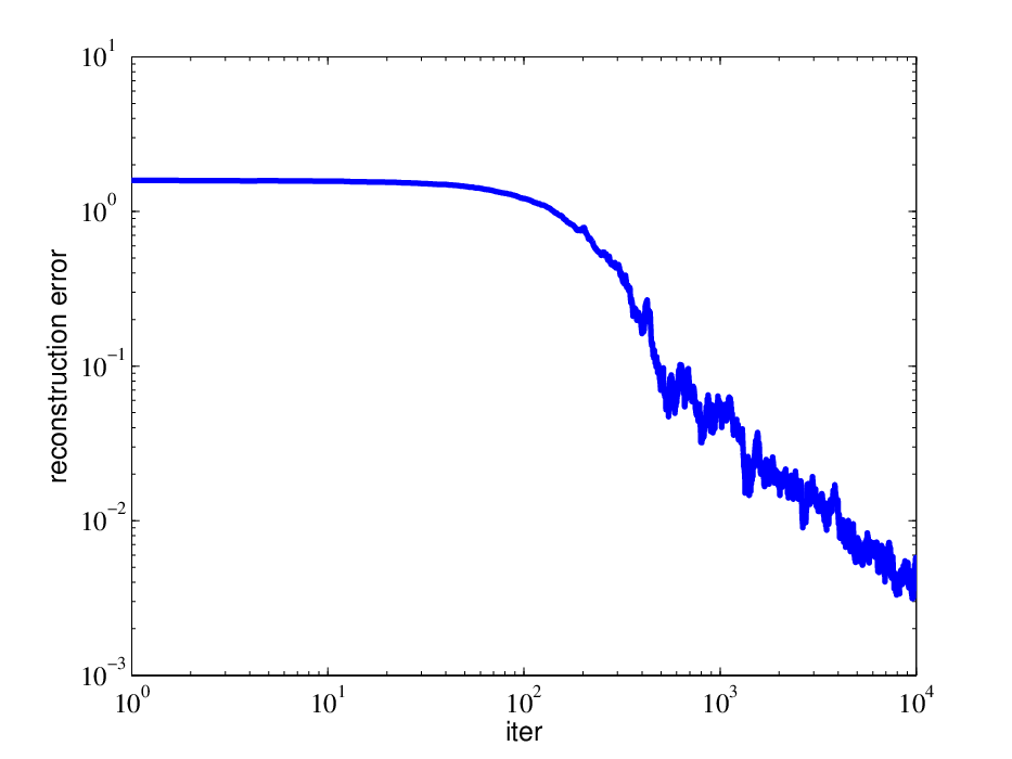
We use the simple way of generating samples for our new objective function (13) and reconstruction error objective (12). The result is shown in Figure 1. Our new objective function is empirically more stable (always converges within 10000 iterations); the reconstruction error do not always converge within the same number of iterations and often exhibits long periods with small improvement (which is likely to be caused by saddle points that do not have a significant negative eigenvalue).

Simple ICA example

As shown in Figure 2, our new algorithm also works in the ICA setting. When the learning rate is constant the error stays at a fixed small value. When we decrease the learning rate the error converges to 0.

Refer to caption
(a) New Objective (13)
Refer to caption
(b) Reconstruction Error Objective (12)
Figure 1: Comparison of different objective functions
Refer to caption
(a) Constant Learning Rate η\eta
Refer to caption
(b) Learning Rate η/t\eta/t (in log\log scale)
Figure 2: ICA setting performance with mini-batch of size 100

6 Conclusion

In this paper we identify the strict saddle property and show stochastic gradient descent converges to a local minimum under this assumption. This leads to new online algorithm for orthogonal tensor decomposition. We hope this is a first step towards understanding stochastic gradient for more classes of non-convex functions. We believe strict saddle property can be extended to handle more functions, especially those functions that have similar symmetry properties.

References

  • Agarwal et al., (2010) Agarwal, A., Negahban, S., and Wainwright, M. J. (2010). Fast global convergence rates of gradient methods for high-dimensional statistical recovery. In Advances in Neural Information Processing Systems, pages 37–45.
  • Anandkumar et al., (2014) Anandkumar, A., Ge, R., Hsu, D., Kakade, S. M., and Telgarsky, M. (2014). Tensor decompositions for learning latent variable models. Journal of Machine Learning Research, 15:2773–2832.
  • Arora et al., (2012) Arora, S., Ge, R., Moitra, A., and Sachdeva, S. (2012). Provable ICA with unknown gaussian noise, with implications for gaussian mixtures and autoencoders. In Advances in Neural Information Processing Systems, pages 2375–2383.
  • Azuma, (1967) Azuma, K. (1967). Weighted sums of certain dependent random variables. Tohoku Mathematical Journal, Second Series, 19(3):357–367.
  • Bengio, (2009) Bengio, Y. (2009). Learning deep architectures for AI. Foundations and trends® in Machine Learning, 2(1):1–127.
  • Cardoso, (1989) Cardoso, J.-F. (1989). Source separation using higher order moments. In Acoustics, Speech, and Signal Processing, pages 2109–2112. IEEE.
  • Choromanska et al., (2014) Choromanska, A., Henaff, M., Mathieu, M., Arous, G. B., and LeCun, Y. (2014). The loss surface of multilayer networks. arXiv:1412.0233.
  • Comon, (2002) Comon, P. (2002). Tensor decompositions. Mathematics in Signal Processing V, pages 1–24.
  • Comon et al., (2009) Comon, P., Luciani, X., and De Almeida, A. L. (2009). Tensor decompositions, alternating least squares and other tales. Journal of Chemometrics, 23(7-8):393–405.
  • Dauphin et al., (2014) Dauphin, Y. N., Pascanu, R., Gulcehre, C., Cho, K., Ganguli, S., and Bengio, Y. (2014). Identifying and attacking the saddle point problem in high-dimensional non-convex optimization. In Advances in Neural Information Processing Systems, pages 2933–2941.
  • Frieze et al., (1996) Frieze, A., Jerrum, M., and Kannan, R. (1996). Learning linear transformations. In 2013 IEEE 54th Annual Symposium on Foundations of Computer Science, pages 359–359.
  • Hanson, (1999) Hanson, M. A. (1999). Invexity and the kuhn–tucker theorem. Journal of mathematical analysis and applications, 236(2):594–604.
  • Harshman, (1970) Harshman, R. A. (1970). Foundations of the PARAFAC procedure: Models and conditions for an “explanatory” multi-modal factor analysis. UCLA Working Papers in Phonetics, 16(1):84.
  • Huang et al., (2013) Huang, F., Niranjan, U., Hakeem, M. U., and Anandkumar, A. (2013). Fast detection of overlapping communities via online tensor methods. arXiv:1309.0787.
  • Hyvarinen, (1999) Hyvarinen, A. (1999). Fast ICA for noisy data using gaussian moments. In Circuits and Systems, volume 5, pages 57–61.
  • Hyvärinen et al., (2004) Hyvärinen, A., Karhunen, J., and Oja, E. (2004). Independent component analysis, volume 46. John Wiley & Sons.
  • Inoue et al., (2003) Inoue, M., Park, H., and Okada, M. (2003). On-line learning theory of soft committee machines with correlated hidden units–steepest gradient descent and natural gradient descent–. Journal of the Physical Society of Japan, 72(4):805–810.
  • Jain et al., (2013) Jain, P., Netrapalli, P., and Sanghavi, S. (2013). Low-rank matrix completion using alternating minimization. In Proceedings of the forty-fifth annual ACM symposium on Theory of computing, pages 665–674.
  • Johnson et al., (1988) Johnson, D. S., Papadimitriou, C. H., and Yannakakis, M. (1988). How easy is local search? Journal of computer and system sciences, 37(1):79–100.
  • Kiwiel, (2001) Kiwiel, K. C. (2001). Convergence and efficiency of subgradient methods for quasiconvex minimization. Mathematical programming, 90(1):1–25.
  • Kolda, (2001) Kolda, T. G. (2001). Orthogonal tensor decompositions. SIAM Journal on Matrix Analysis and Applications, 23(1):243–255.
  • Mangasarian, (1965) Mangasarian, O. L. (1965). Pseudo-convex functions. Journal of the Society for Industrial & Applied Mathematics, Series A: Control, 3(2):281–290.
  • Olshausen and Field, (1997) Olshausen, B. A. and Field, D. J. (1997). Sparse coding with an overcomplete basis set: A strategy employed by V1? Vision research, 37(23):3311–3325.
  • Rakhlin et al., (2012) Rakhlin, A., Shamir, O., and Sridharan, K. (2012). Making gradient descent optimal for strongly convex stochastic optimization. In ICML, pages 449–456.
  • Rattray et al., (1998) Rattray, M., Saad, D., and Amari, S.-i. (1998). Natural gradient descent for on-line learning. Physical review letters, 81(24):5461.
  • Rumelhart et al., (1988) Rumelhart, D. E., Hinton, G. E., and Williams, R. J. (1988). Learning representations by back-propagating errors. Cognitive modeling, 5.
  • Saad and Solla, (1995) Saad, D. and Solla, S. A. (1995). On-line learning in soft committee machines. Physical Review E, 52(4):4225.
  • Saxe et al., (2013) Saxe, A. M., McClelland, J. L., and Ganguli, S. (2013). Exact solutions to the nonlinear dynamics of learning in deep linear neural networks. arXiv:1312.6120.
  • Shalev-Shwartz et al., (2009) Shalev-Shwartz, S., Shamir, O., Sridharan, K., and Srebro, N. (2009). Stochastic convex optimization. In Proceedings of The 22nd Conference on Learning Theory.
  • Wright and Nocedal, (1999) Wright, S. J. and Nocedal, J. (1999). Numerical optimization, volume 2. Springer New York.
  • Zou et al., (2013) Zou, J. Y., Hsu, D., Parkes, D. C., and Adams, R. P. (2013). Contrastive learning using spectral methods. In Advances in Neural Information Processing Systems, pages 2238–2246.

Appendix A Detailed Analysis for Section 3 in Unconstrained Case

In this section we give detailed analysis for noisy gradient descent, under the assumption that the unconstrained problem satisfies (α,γ,ϵ,δ)(\alpha,\gamma,\epsilon,\delta)-strict saddle property.

The algorithm we investigate in Algorithm 1, we can combine the randomness in the stochastic gradient oracle and the artificial noise, and rewrite the update equation in form:

wt=wt−1−η⁡(∇f​(wt−1)+ξt−1)w_{t}=w_{t-1}-\eta(\nabla f(w_{t-1})+\xi_{t-1}) (15)

where η\eta is step size, ξ=S​G​(wt−1)−∇f​(wt−1)+n\xi=SG(w_{t-1})-\nabla f(w_{t-1})+n (recall nn is a random vector on unit sphere) is the combination of two source of noise.

By assumption, we know ξ\xi’s are independent and they satisfying 𝔼​ξ=0\mathbb{E}\xi=0, ‖ξ‖≤Q+1\|\xi\|\leq Q+1. Due to the explicitly added noise in Algorithm 1, we further have 𝔼​ξ​ξT≻1d​I\mathbb{E}\xi\xi^{T}\succ\frac{1}{d}I. For simplicity, we assume 𝔼​ξ​ξT=σ2​I\mathbb{E}\xi\xi^{T}=\sigma^{2}I, for some constant σ=Θ~​(1)\sigma=\tilde{\Theta}(1), then the algorithm we are running is exactly the same as Stochastic Gradient Descent (SGD). Our proof can be very easily extended to the case when 1d​I⪯𝔼⁡[ξ​ξT]⪯(Q+1d)​I\frac{1}{d}I\preceq\mathbb{E}[\xi\xi^{T}]\preceq(Q+\frac{1}{d})I because both the upper and lower bounds are Θ~​(1)\tilde{\Theta}(1).

We first restate the main theorem in the context of stochastic gradient descent.

Theorem 13 (Main Theorem).

Suppose a function f⁡(w):ℝd→ℝf(w):\mathbb{R}^{d}\to\mathbb{R} that is (α,γ,ϵ,δ)(\alpha,\gamma,\epsilon,\delta)-strict saddle, and has a stochastic gradient oracle where the noise satisfy 𝔼​ξ​ξT=σ2​I\mathbb{E}\xi\xi^{T}=\sigma^{2}I. Further, suppose the function is bounded by |f⁡(w)|≤B|f(w)|\leq B, is β\beta-smooth and has ρ\rho-Lipschitz Hessian. Then there exists a threshold ηmax=Θ~​(1)\eta_{\max}=\tilde{\Theta}(1), so that for any ζ>0\zeta>0, and for any η≤ηmax/max⁡{1,log⁡(1/ζ)}\eta\leq\eta_{\max}/\max\{1,\log(1/\zeta)\}, with probability at least 1−ζ1-\zeta in t=O~​(η−2​log⁡(1/ζ))t=\tilde{O}(\eta^{-2}\log(1/\zeta)) iterations, SGD outputs a point wtw_{t} that is O~​(η​log⁡(1/η​ζ))\tilde{O}(\sqrt{\eta\log(1/\eta\zeta)})-close to some local minimum w⋆w^{\star}.

Recall that O~​(⋅)\tilde{O}(\cdot) (Ω~,Θ~\tilde{\Omega},\tilde{\Theta}) hides the factor that is polynomially dependent on all other parameters, but independent of η\eta and ζ\zeta. So it focuses on the dependency on η\eta and ζ\zeta. Throughout the proof, we interchangeably use both ℋ⁡(w)\mathcal{H}(w) and ∇2f​(w)\nabla^{2}f(w) to represent the Hessian matrix of f⁡(w)f(w).

As we discussed in the proof sketch in Section 3, we analyze the behavior of the algorithm in three different cases. The first case is when the gradient is large.

Lemma 14.

Under the assumptions of Theorem 13, for any point with ‖∇f​(w0)‖≥2​η​σ2​β​d\|\nabla f(w_{0})\|\geq\sqrt{2\eta\sigma^{2}\beta d} where 2​η​σ2​β​d<ϵ\sqrt{2\eta\sigma^{2}\beta d}<\epsilon, after one iteration we have:

𝔼​f​(w1)−f⁡(w0)≤−Ω~​(η2)\mathbb{E}f(w_{1})-f(w_{0})\leq-\tilde{\Omega}(\eta^{2}) (16)
Proof.

Choose ηmax<1β\eta_{\max}<\frac{1}{\beta}, then by update equation Eq.(15), we have:

𝔼​f​(w1)−f⁡(w0)\displaystyle\mathbb{E}f(w_{1})-f(w_{0}) ≤∇f(w0)T𝔼(w1−w0)+β2𝔼∥w1−w0∥2\displaystyle\leq\nabla f(w_{0})^{T}\mathbb{E}(w_{1}-w_{0})+\frac{\beta}{2}\mathbb{E}\|w_{1}-w_{0}\|^{2}
=∇f(w0)T𝔼(−η(∇f(w0)+ξ0))+β2𝔼‖−η(∇f(w0)+ξ0)‖2\displaystyle=\nabla f(w_{0})^{T}\mathbb{E}\left(-\eta(\nabla f(w_{0})+\xi_{0})\right)+\frac{\beta}{2}\mathbb{E}\left\|-\eta(\nabla f(w_{0})+\xi_{0})\right\|^{2}
=−(η−β​η22)​‖∇f​(w0)‖2+η2​σ2​β​d2\displaystyle=-(\eta-\frac{\beta\eta^{2}}{2})\|\nabla f(w_{0})\|^{2}+\frac{\eta^{2}\sigma^{2}\beta d}{2}
≤−η2​‖∇f​(w0)‖2+η2​σ2​β​d2≤−η2​σ2​β​d2\displaystyle\leq-\frac{\eta}{2}\|\nabla f(w_{0})\|^{2}+\frac{\eta^{2}\sigma^{2}\beta d}{2}\leq-\frac{\eta^{2}\sigma^{2}\beta d}{2} (17)

which finishes the proof. ∎

Lemma 15.

Under the assumptions of Theorem 13, for any initial point w0w_{0} that is O~​(η)<δ\tilde{O}(\sqrt{\eta})<\delta close to a local minimum w⋆w^{\star}, with probability at least 1−ζ/21-\zeta/2, we have following holds simultaneously:

∀t≤O~​(1η2​log⁡1ζ),‖wt−w⋆‖≤O~​(η​log⁡1η​ζ)<δ\forall t\leq\tilde{O}(\frac{1}{\eta^{2}}\log\frac{1}{\zeta}),\quad\|w_{t}-w^{\star}\|\leq\tilde{O}(\sqrt{\eta\log\frac{1}{\eta\zeta}})<\delta (18)

where w⋆w^{\star} is the locally optimal point.

Proof.

We shall construct a supermartingale and use Azuma’s inequality (Azuma,, 1967) to prove this result.

Let filtration 𝔉t=σ{ξ0,⋯ξt−1}\mathfrak{F}_{t}=\sigma\{\xi_{0},\cdots\xi_{t-1}\}, and note σ⁡{Δ0,⋯,Δt}⊂𝔉t\sigma\{\Delta_{0},\cdots,\Delta_{t}\}\subset\mathfrak{F}_{t}, where σ​{⋅}\sigma\{\cdot\} denotes the sigma field. Let event 𝔈t={∀τ≤t,∥wτ−w⋆∥≤μη​log⁡1η​ζ<δ}\mathfrak{E}_{t}=\{\forall\tau\leq t,\|w_{\tau}-w^{\star}\|\leq\mu\sqrt{\eta\log\frac{1}{\eta\zeta}}<\delta\}, where μ\mu is independent of (η,ζ)(\eta,\zeta), and will be specified later. To ensure the correctness of proof, O~\tilde{O} notation in this proof will never hide any dependence on μ\mu. Clearly there’s always a small enough choice of ηmax=Θ~​(1)\eta_{\max}=\tilde{\Theta}(1) to make μ​η​log⁡1η​ζ<δ\mu\sqrt{\eta\log\frac{1}{\eta\zeta}}<\delta holds as long as η≤ηmax/max⁡{1,log⁡(1/ζ)}\eta\leq\eta_{\max}/\max\{1,\log(1/\zeta)\}. Also note 𝔈t⊂𝔈t−1\mathfrak{E}_{t}\subset\mathfrak{E}_{t-1}, that is 1𝔈t≤1𝔈t−11_{\mathfrak{E}_{t}}\leq 1_{\mathfrak{E}_{t-1}}.

By Definition 5 of (α,γ,ϵ,δ)(\alpha,\gamma,\epsilon,\delta)-strict saddle, we know ff is locally α\alpha-strongly convex in the 2​δ2\delta-neighborhood of w⋆w^{\star}. Since ∇f​(w⋆)=0\nabla f(w^{\star})=0, we have

∇f(wt)T(wt−w⋆)1𝔈t≥α∥wt−w⋆∥21𝔈t\displaystyle\nabla f(w_{t})^{T}(w_{t}-w^{\star})1_{\mathfrak{E}_{t}}\geq\alpha\|w_{t}-w^{\star}\|^{2}1_{\mathfrak{E}_{t}} (19)

Furthermore, with ηmax<αβ2\eta_{\max}<\frac{\alpha}{\beta^{2}}, using β\beta-smoothness, we have:

𝔼⁡[‖wt−w⋆‖2​1𝔈t−1|𝔉t−1]=\displaystyle\mathbb{E}[\|w_{t}-w^{\star}\|^{2}1_{\mathfrak{E}_{t-1}}|\mathfrak{F}_{t-1}]= 𝔼⁡[‖wt−1−η⁡(∇f​(wt−1)+ξt−1)−w⋆‖2|𝔉t−1]​1𝔈t−1\displaystyle\mathbb{E}[\|w_{t-1}-\eta(\nabla f(w_{t-1})+\xi_{t-1})-w^{\star}\|^{2}|\mathfrak{F}_{t-1}]1_{\mathfrak{E}_{t-1}}
=\displaystyle= [∥wt−1−w⋆∥2−2η∇f(wt−1)T(wt−1−w⋆)+η2∥∇f(wt−1)∥2+η2σ2]1𝔈t−1\displaystyle\left[\|w_{t-1}-w^{\star}\|^{2}-2\eta\nabla f(w_{t-1})^{T}(w_{t-1}-w^{\star})+\eta^{2}\|\nabla f(w_{t-1})\|^{2}+\eta^{2}\sigma^{2}\right]1_{\mathfrak{E}_{t-1}}
≤\displaystyle\leq [(1−2​η​α+η2​β2)​‖wt−1−w⋆‖2+η2​σ2]​1𝔈t−1\displaystyle[(1-2\eta\alpha+\eta^{2}\beta^{2})\|w_{t-1}-w^{\star}\|^{2}+\eta^{2}\sigma^{2}]1_{\mathfrak{E}_{t-1}}
≤\displaystyle\leq [(1−η​α)​‖wt−1−w⋆‖2+η2​σ2]​1𝔈t−1\displaystyle[(1-\eta\alpha)\|w_{t-1}-w^{\star}\|^{2}+\eta^{2}\sigma^{2}]1_{\mathfrak{E}_{t-1}} (20)

Therefore, we have:

[𝔼⁡[‖wt−w⋆‖2|𝔉t−1]−ηα]​1𝔈t−1≤(1−η​α)​[‖wt−1−w⋆‖2−ηα]​1𝔈t−1\left[\mathbb{E}[\|w_{t}-w^{\star}\|^{2}|\mathfrak{F}_{t-1}]-\frac{\eta}{\alpha}\right]1_{\mathfrak{E}_{t-1}}\leq(1-\eta\alpha)\left[\|w_{t-1}-w^{\star}\|^{2}-\frac{\eta}{\alpha}\right]1_{\mathfrak{E}_{t-1}} (21)

Then, let Gt=(1−η​α)−t​(‖wt−w⋆‖2−ηα)G_{t}=(1-\eta\alpha)^{-t}(\|w_{t}-w^{\star}\|^{2}-\frac{\eta}{\alpha}), we have:

𝔼⁡[Gt​1𝔈t−1|𝔉t−1]≤Gt−1​1𝔈t−1≤Gt−1​1𝔈t−2\mathbb{E}[G_{t}1_{\mathfrak{E}_{t-1}}|\mathfrak{F}_{t-1}]\leq G_{t-1}1_{\mathfrak{E}_{t-1}}\leq G_{t-1}1_{\mathfrak{E}_{t-2}} (22)

which means Gt​1𝔈t−1G_{t}1_{\mathfrak{E}_{t-1}} is a supermartingale.

Therefore, with probability 1, we have:

|Gt​1𝔈t−1−𝔼⁡[Gt​1𝔈t−1|𝔉t−1]|\displaystyle|G_{t}1_{\mathfrak{E}_{t-1}}-\mathbb{E}[G_{t}1_{\mathfrak{E}_{t-1}}|\mathfrak{F}_{t-1}]|
≤\displaystyle\leq (1−ηα)−t[∥wt−1−η∇f(wt−1)−w⋆∥⋅η∥ξt−1∥+η2∥ξt−1∥2−η2σ2]1𝔈t−1\displaystyle(1-\eta\alpha)^{-t}[~\|w_{t-1}-\eta\nabla f(w_{t-1})-w^{\star}\|\cdot\eta\|\xi_{t-1}\|+\eta^{2}\|\xi_{t-1}\|^{2}-\eta^{2}\sigma^{2}~]1_{\mathfrak{E}_{t-1}}
≤\displaystyle\leq (1−η​α)−t⋅O~​(μ​η1.5​log12​1η​ζ)=dt\displaystyle(1-\eta\alpha)^{-t}\cdot\tilde{O}(\mu\eta^{1.5}\log^{\frac{1}{2}}\frac{1}{\eta\zeta})=d_{t} (23)

Let

ct=∑τ=1tdτ2=O~​(μ​η1.5​log12​1η​ζ)​∑τ=1t(1−η​α)−2​τc_{t}=\sqrt{\sum_{\tau=1}^{t}d_{\tau}^{2}}=\tilde{O}(\mu\eta^{1.5}\log^{\frac{1}{2}}\frac{1}{\eta\zeta})\sqrt{\sum_{\tau=1}^{t}(1-\eta\alpha)^{-2\tau}} (24)

By Azuma’s inequality, with probability less than O~​(η3​ζ)\tilde{O}(\eta^{3}\zeta), we have:

Gt​1𝔈t−1>O~​(1)​ct​log12⁡(1η​ζ)+G0\displaystyle G_{t}1_{\mathfrak{E}_{t-1}}>\tilde{O}(1)c_{t}\log^{\frac{1}{2}}(\frac{1}{\eta\zeta})+G_{0} (25)

We know Gt>O~​(1)​ct​log12⁡(1η​ζ)+G0G_{t}>\tilde{O}(1)c_{t}\log^{\frac{1}{2}}(\frac{1}{\eta\zeta})+G_{0} is equivalent to:

‖wt−w⋆‖2>O~​(η)+O~​(1)​(1−η​α)t​ct​log12⁡(1η​ζ)\displaystyle\|w_{t}-w^{\star}\|^{2}>\tilde{O}(\eta)+\tilde{O}(1)(1-\eta\alpha)^{t}c_{t}\log^{\frac{1}{2}}(\frac{1}{\eta\zeta}) (26)

We know:

(1−η​α)t​ct​log12⁡(1η​ζ)=μ⋅O~​(η1.5​log⁡1η​ζ)​∑τ=1t(1−η​α)2​(t−τ)\displaystyle(1-\eta\alpha)^{t}c_{t}\log^{\frac{1}{2}}(\frac{1}{\eta\zeta})=\mu\cdot\tilde{O}(\eta^{1.5}\log\frac{1}{\eta\zeta})\sqrt{\sum_{\tau=1}^{t}(1-\eta\alpha)^{2(t-\tau)}}
=\displaystyle= μ⋅O~​(η1.5​log⁡1η​ζ)​∑τ=0t−1(1−η​α)2​τ≤μ⋅O~​(η1.5​log⁡1η​ζ)​11−(1−η​α)2=μ⋅O~​(η​log⁡1η​ζ)\displaystyle\mu\cdot\tilde{O}(\eta^{1.5}\log\frac{1}{\eta\zeta})\sqrt{\sum_{\tau=0}^{t-1}(1-\eta\alpha)^{2\tau}}\leq\mu\cdot\tilde{O}(\eta^{1.5}\log\frac{1}{\eta\zeta})\sqrt{\frac{1}{1-(1-\eta\alpha)^{2}}}=\mu\cdot\tilde{O}(\eta\log\frac{1}{\eta\zeta}) (27)

This means Azuma’s inequality implies, there exist some C~=O~​(1)\tilde{C}=\tilde{O}(1) so that:

P(𝔈t−1∩{∥wt−w⋆∥2>μ⋅C~ηlog1η​ζ)})≤O~(η3ζ)\displaystyle P\left(\mathfrak{E}_{t-1}\cap\left\{\|w_{t}-w^{\star}\|^{2}>\mu\cdot\tilde{C}\eta\log\frac{1}{\eta\zeta})\right\}\right)\leq\tilde{O}(\eta^{3}\zeta) (28)

By choosing μ>C~\mu>\tilde{C}, this is equivalent to:

P(𝔈t−1∩{∥wt−w⋆∥2>μ2ηlog1η​ζ})≤O~(η3ζ)\displaystyle P\left(\mathfrak{E}_{t-1}\cap\left\{\|w_{t}-w^{\star}\|^{2}>\mu^{2}\eta\log\frac{1}{\eta\zeta}\right\}\right)\leq\tilde{O}(\eta^{3}\zeta) (29)

Then we have:

P(𝔈¯t)=P(𝔈t−1∩{∥wt−w⋆∥>μη​log⁡1η​ζ})+P(𝔈¯t−1)≤O~(η3ζ)+P(𝔈¯t−1)\displaystyle P(\overline{\mathfrak{E}}_{t})=P\left(\mathfrak{E}_{t-1}\cap\left\{\|w_{t}-w^{\star}\|>\mu\sqrt{\eta\log\frac{1}{\eta\zeta}}\right\}\right)+P(\overline{\mathfrak{E}}_{t-1})\leq\tilde{O}(\eta^{3}\zeta)+P(\overline{\mathfrak{E}}_{t-1}) (30)

By initialization conditions, we know P⁡(𝔈¯0)=0P(\overline{\mathfrak{E}}_{0})=0, and thus P⁡(𝔈¯t)≤t​O~​(η3​ζ)P(\overline{\mathfrak{E}}_{t})\leq t\tilde{O}(\eta^{3}\zeta). Take t=O~​(1η2​log⁡1ζ)t=\tilde{O}(\frac{1}{\eta^{2}}\log\frac{1}{\zeta}), we have P⁡(𝔈¯t)≤O~​(η​ζ​log⁡1ζ)P(\overline{\mathfrak{E}}_{t})\leq\tilde{O}(\eta\zeta\log\frac{1}{\zeta}). When ηmax=O~​(1)\eta_{\max}=\tilde{O}(1) is chosen small enough, and η≤ηmax/log⁡(1/ζ)\eta\leq\eta_{\max}/\log(1/\zeta), this finishes the proof. ∎

Lemma 16.

Under the assumptions of Theorem 13, for any initial point w0w_{0} where ‖∇f​(w0)‖≤2​η​σ2​β​d<ϵ\|\nabla f(w_{0})\|\leq\sqrt{2\eta\sigma^{2}\beta d}<\epsilon, and λmin​(ℋ⁡(w0))≤−γ\lambda_{\min}(\mathcal{H}(w_{0}))\leq-\gamma, then there is a number of steps TT that depends on w0w_{0} such that:

𝔼​f​(wT)−f⁡(w0)≤−Ω~​(η)\mathbb{E}f(w_{T})-f(w_{0})\leq-\tilde{\Omega}(\eta) (31)

The number of steps TT has a fixed upper bound Tm​a​xT_{max} that is independent of w0w_{0} where T≤Tm​a​x=O⁡((log⁡d)/γ​η)T\leq T_{max}=O((\log d)/\gamma\eta).

Remark.

In general, if we relax the assumption 𝔼​ξ​ξT=σ2​I\mathbb{E}\xi\xi^{T}=\sigma^{2}I to σmin2​I⪯𝔼​ξ​ξT⪯σmax2​I\sigma_{\min}^{2}I\preceq\mathbb{E}\xi\xi^{T}\preceq\sigma_{\max}^{2}I, the upper bound Tm​a​xT_{max} of number of steps required in Lemma 16 would be increased to Tm​a​x=O⁡(1γ​η​(log⁡d+log⁡σmaxσmin))T_{max}=O(\frac{1}{\gamma\eta}(\log d+\log\frac{\sigma_{\max}}{\sigma_{\min}}))

As we described in the proof sketch, the main idea is to consider a coupled update sequence that correspond to the local second-order approximation of f⁡(x)f(x) around w0w_{0}. We characterize this sequence of update in the next lemma.

Lemma 17.

Under the assumptions of Theorem 13. Let f~\tilde{f} defined as local second-order approximation of f⁡(x)f(x) around w0w_{0}:

f~(w)≐f(w0)+∇f(w0)T(w−w0)+12(w−w0)Tℋ(w0)(w−w0)\tilde{f}(w)\doteq f(w_{0})+\nabla f(w_{0})^{T}(w-w_{0})+\frac{1}{2}(w-w_{0})^{T}\mathcal{H}(w_{0})(w-w_{0}) (32)

{w~t}\{\tilde{w}_{t}\} be the corresponding sequence generated by running SGD on function f~\tilde{f}, with w~0=w0\tilde{w}_{0}=w_{0}. For simplicity, denote ℋ=ℋ⁡(w0)=∇2f​(w0)\mathcal{H}=\mathcal{H}(w_{0})=\nabla^{2}f(w_{0}), then we have analytically:

∇f~(w~t)=(1−ηℋ)t∇f(w0)−ηℋ∑τ=0t−1(1−ηℋ)t−τ−1ξτ\displaystyle\nabla\tilde{f}(\tilde{w}_{t})=(1-\eta\mathcal{H})^{t}\nabla f(w_{0})-\eta\mathcal{H}\sum_{\tau=0}^{t-1}(1-\eta\mathcal{H})^{t-\tau-1}\xi_{\tau} (33)
w~t−w0=−η∑τ=0t−1(1−ηℋ)τ∇f(w0)−η∑τ=0t−1(1−ηℋ)t−τ−1ξτ\displaystyle\tilde{w}_{t}-w_{0}=-\eta\sum_{\tau=0}^{t-1}(1-\eta\mathcal{H})^{\tau}\nabla f(w_{0})-\eta\sum_{\tau=0}^{t-1}(1-\eta\mathcal{H})^{t-\tau-1}\xi_{\tau} (34)

Furthermore, for any initial point w0w_{0} where ‖∇f​(w0)‖≤O~​(η)<ϵ\|\nabla f(w_{0})\|\leq\tilde{O}(\eta)<\epsilon, and λmin​(ℋ⁡(w0))=−γ0\lambda_{\min}(\mathcal{H}(w_{0}))=-\gamma_{0}. Then, there exist a T∈ℕT\in\mathbb{N} satisfying:

dη​γ0≤∑τ=0T−1(1+η​γ0)2​τ<3​dη​γ0\frac{d}{\eta\gamma_{0}}\leq\sum_{\tau=0}^{T-1}(1+\eta\gamma_{0})^{2\tau}<\frac{3d}{\eta\gamma_{0}} (35)

with probability at least 1−O~​(η3)1-\tilde{O}(\eta^{3}), we have following holds simultaneously for all t≤Tt\leq T:

‖w~t−w0‖≤O~​(η12​log⁡1η);‖∇f~​(w~t)‖≤O~​(η12​log⁡1η)\|\tilde{w}_{t}-w_{0}\|\leq\tilde{O}(\eta^{\frac{1}{2}}\log\frac{1}{\eta});\quad\quad\|\nabla\tilde{f}(\tilde{w}_{t})\|\leq\tilde{O}(\eta^{\frac{1}{2}}\log\frac{1}{\eta}) (36)
Proof.

Denote ℋ=ℋ⁡(w0)\mathcal{H}=\mathcal{H}(w_{0}), since f~\tilde{f} is quadratic, clearly we have:

∇f~​(w~t)=∇f~​(w~t−1)+ℋ⁡(w~t−w~t−1)\nabla\tilde{f}(\tilde{w}_{t})=\nabla\tilde{f}(\tilde{w}_{t-1})+\mathcal{H}(\tilde{w}_{t}-\tilde{w}_{t-1}) (37)

Substitute the update equation of SGD in Eq.(37), we have:

∇f~​(w~t)\displaystyle\nabla\tilde{f}(\tilde{w}_{t}) =∇f~​(w~t−1)−η​ℋ​(∇f~​(w~t−1)+ξt−1)\displaystyle=\nabla\tilde{f}(\tilde{w}_{t-1})-\eta\mathcal{H}(\nabla\tilde{f}(\tilde{w}_{t-1})+\xi_{t-1})
=(1−ηℋ)∇f~(w~t−1)−ηℋξt−1\displaystyle=(1-\eta\mathcal{H})\nabla\tilde{f}(\tilde{w}_{t-1})-\eta\mathcal{H}\xi_{t-1}
=(1−ηℋ)2∇f~(w~t−2)−ηℋξt−1−ηℋ(1−ηℋ)ξt−2=⋯\displaystyle=(1-\eta\mathcal{H})^{2}\nabla\tilde{f}(\tilde{w}_{t-2})-\eta\mathcal{H}\xi_{t-1}-\eta\mathcal{H}(1-\eta\mathcal{H})\xi_{t-2}=\cdots
=(1−ηℋ)t∇f(w0)−ηℋ∑τ=0t−1(1−ηℋ)t−τ−1ξτ\displaystyle=(1-\eta\mathcal{H})^{t}\nabla f(w_{0})-\eta\mathcal{H}\sum_{\tau=0}^{t-1}(1-\eta\mathcal{H})^{t-\tau-1}\xi_{\tau} (38)

Therefore, we have:

w~t−w0\displaystyle\tilde{w}_{t}-w_{0} =−η∑τ=0t−1(∇f~(w~τ)+ξτ)\displaystyle=-\eta\sum_{\tau=0}^{t-1}(\nabla\tilde{f}(\tilde{w}_{\tau})+\xi_{\tau})
=−η∑τ=0t−1((1−ηℋ)τ∇f(w0)−ηℋ∑τ′=0τ−1(1−ηℋ)τ−τ′−1ξτ′+ξτ)\displaystyle=-\eta\sum_{\tau=0}^{t-1}\left((1-\eta\mathcal{H})^{\tau}\nabla f(w_{0})-\eta\mathcal{H}\sum_{\tau^{\prime}=0}^{\tau-1}(1-\eta\mathcal{H})^{\tau-\tau^{\prime}-1}\xi_{\tau^{\prime}}+\xi_{\tau}\right)
=−η∑τ=0t−1(1−ηℋ)τ∇f(w0)−η∑τ=0t−1(1−ηℋ)t−τ−1ξτ\displaystyle=-\eta\sum_{\tau=0}^{t-1}(1-\eta\mathcal{H})^{\tau}\nabla f(w_{0})-\eta\sum_{\tau=0}^{t-1}(1-\eta\mathcal{H})^{t-\tau-1}\xi_{\tau} (39)

Next, we prove the existence of TT in Eq.(35). Since ∑τ=0t(1+η​γ0)2​τ\sum_{\tau=0}^{t}(1+\eta\gamma_{0})^{2\tau} is monotonically increasing w.r.t tt, and diverge to infinity as t→∞t\rightarrow\infty. We know there is always some T∈ℕT\in\mathbb{N} gives dη​γ0≤∑τ=0T−1(1+η​γ0)2​τ\frac{d}{\eta\gamma_{0}}\leq\sum_{\tau=0}^{T-1}(1+\eta\gamma_{0})^{2\tau}. Let TT be the smallest integer satisfying above equation. By assumption, we know γ≤γ0≤L\gamma\leq\gamma_{0}\leq L, and

∑τ=0t+1(1+η​γ0)2​τ=1+(1+η​γ0)2​∑τ=0t(1+η​γ0)2​τ\sum_{\tau=0}^{t+1}(1+\eta\gamma_{0})^{2\tau}=1+(1+\eta\gamma_{0})^{2}\sum_{\tau=0}^{t}(1+\eta\gamma_{0})^{2\tau} (40)

we can choose ηmax<min⁡{(2−1)/L,2​d/γ}\eta_{\max}<\min\{(\sqrt{2}-1)/L,2d/\gamma\} so that

dη​γ0≤∑τ=0T−1(1+η​γ0)2​τ≤1+2​dη​γ0≤3​dη​γ0\frac{d}{\eta\gamma_{0}}\leq\sum_{\tau=0}^{T-1}(1+\eta\gamma_{0})^{2\tau}\leq 1+\frac{2d}{\eta\gamma_{0}}\leq\frac{3d}{\eta\gamma_{0}} (41)

Finally, by Eq.(35), we know T=O⁡(log⁡d/γ0​η)T=O(\log d/\gamma_{0}\eta), and (1+η​γ0)T≤O~​(1)(1+\eta\gamma_{0})^{T}\leq\tilde{O}(1). Also because 𝔼​ξ=0\mathbb{E}\xi=0 and ‖ξ‖≤Q=O~​(1)\|\xi\|\leq Q=\tilde{O}(1) with probability 1, then by Hoeffding inequality, we have for each dimension ii and time t≤Tt\leq T:

P⁡(|η​∑τ=0t−1(1−η​ℋ)t−τ−1​ξτ,i|>O~​(η12​log⁡1η))≤e−Ω~​(log2⁡1η)≤O~​(η4)P\left(|\eta\sum_{\tau=0}^{t-1}(1-\eta\mathcal{H})^{t-\tau-1}\xi_{\tau,i}|>\tilde{O}(\eta^{\frac{1}{2}}\log{\frac{1}{\eta}})\right)\leq e^{-\tilde{\Omega}(\log^{2}\frac{1}{\eta})}\leq\tilde{O}(\eta^{4}) (42)

then by summing over dimension dd and taking union bound over all t≤Tt\leq T, we directly have:

P(∀t≤T,∥η∑τ=0t−1(1−ηℋ)t−τ−1ξτ∥>O~(η12log1η))≤O~(η3).P\left(\forall t\leq T,\|\eta\sum_{\tau=0}^{t-1}(1-\eta\mathcal{H})^{t-\tau-1}\xi_{\tau}\|>\tilde{O}(\eta^{\frac{1}{2}}\log\frac{1}{\eta})\right)\leq\tilde{O}(\eta^{3}). (43)

Combine this fact with Eq.(38) and Eq.(39), we finish the proof.

∎

Next we need to prove that the two sequences of updates are always close.

Lemma 18.

Under the assumptions of Theorem 13. and let {wt}\{w_{t}\} be the corresponding sequence generated by running SGD on function ff. Also let f~\tilde{f} and {w~t}\{\tilde{w}_{t}\} be defined as in Lemma 17. Then, for any initial point w0w_{0} where ‖∇f​(w0)‖≤O~​(η)<ϵ\|\nabla f(w_{0})\|\leq\tilde{O}(\eta)<\epsilon, and λmin​(∇2f​(w0))=−γ0\lambda_{\min}(\nabla^{2}f(w_{0}))=-\gamma_{0}. Given the choice of TT as in Eq.(35), with probability at least 1−O~​(η2)1-\tilde{O}(\eta^{2}), we have following holds simultaneously for all t≤Tt\leq T:

‖wt−w~t‖≤O~​(η​log2​1η);‖∇f​(wt)−∇f~​(w~t)‖≤O~​(η​log2​1η)\displaystyle\|w_{t}-\tilde{w}_{t}\|\leq\tilde{O}(\eta\log^{2}\frac{1}{\eta});\quad\quad\|\nabla f(w_{t})-\nabla\tilde{f}(\tilde{w}_{t})\|\leq\tilde{O}(\eta\log^{2}\frac{1}{\eta}) (44)
Proof.

First, we have update function of gradient by:

∇f​(wt)=\displaystyle\nabla f(w_{t})= ∇f​(wt−1)+∫01ℋ⁡(wt−1+t⁡(wt−wt−1))​𝑑t⋅(wt−wt−1)\displaystyle\nabla f(w_{t-1})+\int_{0}^{1}\mathcal{H}(w_{t-1}+t(w_{t}-w_{t-1}))\mathrm{d}t\cdot(w_{t}-w_{t-1})
=\displaystyle= ∇f​(wt−1)+ℋ⁡(wt−1)​(wt−wt−1)+θt−1\displaystyle\nabla f(w_{t-1})+\mathcal{H}(w_{t-1})(w_{t}-w_{t-1})+\theta_{t-1} (45)

where the remainder:

θt−1≡∫01[ℋ⁡(wt−1+t⁡(wt−wt−1))−ℋ⁡(wt−1)]​𝑑t⋅(wt−wt−1)\theta_{t-1}\equiv\int_{0}^{1}\left[\mathcal{H}(w_{t-1}+t(w_{t}-w_{t-1}))-\mathcal{H}(w_{t-1})\right]\mathrm{d}t\cdot(w_{t}-w_{t-1}) (46)

Denote ℋ=ℋ⁡(w0)\mathcal{H}=\mathcal{H}(w_{0}), and ℋt−1′=ℋ⁡(wt−1)−ℋ⁡(w0)\mathcal{H}^{\prime}_{t-1}=\mathcal{H}(w_{t-1})-\mathcal{H}(w_{0}). By Hessian smoothness, we immediately have:

‖ℋt−1′‖=‖ℋ⁡(wt−1)−ℋ⁡(w0)‖≤ρ|wt−1−w0|≤ρ⁡(‖wt−w~t‖+‖w~t−w0‖)\displaystyle\|\mathcal{H}^{\prime}_{t-1}\|=\|\mathcal{H}(w_{t-1})-\mathcal{H}(w_{0})\|\leq\rho\|w_{t-1}-w_{0}\|\leq\rho(\|w_{t}-\tilde{w}_{t}\|+\|\tilde{w}_{t}-w_{0}\|) (47)
‖θt−1‖≤ρ2​‖wt−wt−1‖2\displaystyle\|\theta_{t-1}\|\leq\frac{\rho}{2}\|w_{t}-w_{t-1}\|^{2} (48)

Substitute the update equation of SGD (Eq.(15)) into Eq.(45), we have:

∇f​(wt)\displaystyle\nabla f(w_{t}) =∇f​(wt−1)−η⁡(ℋ+ℋt−1′)​(∇f​(wt−1)+ξt−1)+θt−1\displaystyle=\nabla f(w_{t-1})-\eta(\mathcal{H}+\mathcal{H}^{\prime}_{t-1})(\nabla f(w_{t-1})+\xi_{t-1})+\theta_{t-1}
=(1−ηℋ)∇f(wt−1)−ηℋξt−1−ηℋt−1′(∇f(wt−1)+ξt−1)+θt−1\displaystyle=(1-\eta\mathcal{H})\nabla f(w_{t-1})-\eta\mathcal{H}\xi_{t-1}-\eta\mathcal{H}^{\prime}_{t-1}(\nabla f(w_{t-1})+\xi_{t-1})+\theta_{t-1} (49)

Let Δt=∇f​(wt)−∇f~​(w~t)\Delta_{t}=\nabla f(w_{t})-\nabla\tilde{f}(\tilde{w}_{t}) denote the difference in gradient, then from Eq.(38), Eq.(49), and Eq.(15), we have:

Δt=(1−η​ℋ)​Δt−1−η​ℋt−1′​[Δt−1+∇f~​(w~t−1)+ξt−1]+θt−1\displaystyle\Delta_{t}=(1-\eta\mathcal{H})\Delta_{t-1}-\eta\mathcal{H}^{\prime}_{t-1}[\Delta_{t-1}+\nabla\tilde{f}(\tilde{w}_{t-1})+\xi_{t-1}]+\theta_{t-1} (50)
wt−w~t=−η∑τ=0t−1Δτ\displaystyle w_{t}-\tilde{w}_{t}=-\eta\sum_{\tau=0}^{t-1}\Delta_{\tau} (51)

Let filtration 𝔉t=σ{ξ0,⋯ξt−1}\mathfrak{F}_{t}=\sigma\{\xi_{0},\cdots\xi_{t-1}\}, and note σ⁡{Δ0,⋯,Δt}⊂𝔉t\sigma\{\Delta_{0},\cdots,\Delta_{t}\}\subset\mathfrak{F}_{t}, where σ​{⋅}\sigma\{\cdot\} denotes the sigma field. Also, let event 𝔎t={∀τ≤t,∥∇f~(w~τ)∥≤O~(η12log1η),∥w~τ−w0∥≤O~(η12log1η)}\mathfrak{K}_{t}=\{\forall\tau\leq t,~\|\nabla\tilde{f}(\tilde{w}_{\tau})\|\leq\tilde{O}(\eta^{\frac{1}{2}}\log\frac{1}{\eta}),~\|\tilde{w}_{\tau}-w_{0}\|\leq\tilde{O}(\eta^{\frac{1}{2}}\log\frac{1}{\eta})\}, and 𝔈t={∀τ≤t,∥Δτ∥≤μηlog21η}\mathfrak{E}_{t}=\{\forall\tau\leq t,~\|\Delta_{\tau}\|\leq\mu\eta\log^{2}\frac{1}{\eta}\}, where μ\mu is independent of (η,ζ)(\eta,\zeta), and will be specified later. Again, O~\tilde{O} notation in this proof will never hide any dependence on μ\mu. Clearly, we have 𝔎t⊂𝔎t−1\mathfrak{K}_{t}\subset\mathfrak{K}_{t-1} (𝔈t⊂𝔈t−1\mathfrak{E}_{t}\subset\mathfrak{E}_{t-1}), thus 1𝔎t≤1𝔎t−11_{\mathfrak{K}_{t}}\leq 1_{\mathfrak{K}_{t-1}} (1𝔈t≤1𝔈t−11_{\mathfrak{E}_{t}}\leq 1_{\mathfrak{E}_{t-1}}), where 1𝔎1_{\mathfrak{K}} is the indicator function of event 𝔎\mathfrak{K}.

We first need to carefully bounded all terms in Eq.(50), conditioned on event 𝔎t−1∩𝔈t−1\mathfrak{K}_{t-1}\cap\mathfrak{E}_{t-1}, by Eq.(47), Eq.(48)), and Eq.(51), with probability 1, for all t≤T≤O⁡(log⁡d/γ0​η)t\leq T\leq O(\log d/\gamma_{0}\eta), we have:

‖(1−η​ℋ)​Δt−1‖≤O~​(μ​η​log2​1η)\displaystyle\|(1-\eta\mathcal{H})\Delta_{t-1}\|\leq\tilde{O}(\mu\eta\log^{2}\frac{1}{\eta}) ‖η​ℋt−1′​(Δt−1+∇f~​(w~t−1))‖≤O~​(η2​log2​1η)\displaystyle\quad\quad\|\eta\mathcal{H}^{\prime}_{t-1}(\Delta_{t-1}+\nabla\tilde{f}(\tilde{w}_{t-1}))\|\leq\tilde{O}(\eta^{2}\log^{2}\frac{1}{\eta})
‖η​ℋt−1′​ξt−1‖≤O~​(η1.5​log⁡1η)\displaystyle\|\eta\mathcal{H}^{\prime}_{t-1}\xi_{t-1}\|\leq\tilde{O}(\eta^{1.5}\log\frac{1}{\eta}) ‖θt−1‖≤O~​(η2)\displaystyle\quad\quad\|\theta_{t-1}\|\leq\tilde{O}(\eta^{2}) (52)

Since event 𝔎t−1⊂𝔉t−1,𝔈t−1⊂𝔉t−1\mathfrak{K}_{t-1}\subset\mathfrak{F}_{t-1},\mathfrak{E}_{t-1}\subset\mathfrak{F}_{t-1} thus independent of ξt−1\xi_{t-1}, we also have:

𝔼⁡[((1−η​ℋ)​Δt−1)T​η​ℋt−1′​ξt−1​1𝔎t−1∩𝔈t−1|𝔉t−1]\displaystyle\mathbb{E}[((1-\eta\mathcal{H})\Delta_{t-1})^{T}\eta\mathcal{H}^{\prime}_{t-1}\xi_{t-1}1_{\mathfrak{K}_{t-1}\cap\mathfrak{E}_{t-1}}~|~\mathfrak{F}_{t-1}]
=\displaystyle= 1𝔎t−1∩𝔈t−1​((1−η​ℋ)​Δt−1)T​η​ℋt−1′​𝔼​[ξt−1|𝔉t−1]=0\displaystyle 1_{\mathfrak{K}_{t-1}\cap\mathfrak{E}_{t-1}}((1-\eta\mathcal{H})\Delta_{t-1})^{T}\eta\mathcal{H}^{\prime}_{t-1}\mathbb{E}[\xi_{t-1}~|~\mathfrak{F}_{t-1}]=0 (53)

Therefore, from Eq.(50) and Eq.(52):

𝔼⁡[‖Δt‖22​1𝔎t−1∩𝔈t−1|𝔉t−1]\displaystyle\mathbb{E}[\|\Delta_{t}\|^{2}_{2}1_{\mathfrak{K}_{t-1}\cap\mathfrak{E}_{t-1}}~|~\mathfrak{F}_{t-1}]
≤\displaystyle\leq [(1+η​γ0)2​‖Δt−1‖2+(1+η​γ0)​‖Δt−1‖​O~​(η2​log2​1η)+O~​(η3​log2​1η)]​1𝔎t−1∩𝔈t−1\displaystyle\left[(1+\eta\gamma_{0})^{2}\|\Delta_{t-1}\|^{2}+(1+\eta\gamma_{0})\|\Delta_{t-1}\|\tilde{O}(\eta^{2}\log^{2}\frac{1}{\eta})+\tilde{O}(\eta^{3}\log^{2}\frac{1}{\eta})\right]1_{\mathfrak{K}_{t-1}\cap\mathfrak{E}_{t-1}}
≤\displaystyle\leq [(1+η​γ0)2​‖Δt−1‖2+O~​(μ​η3​log4​1η)]​1𝔎t−1∩𝔈t−1\displaystyle\left[(1+\eta\gamma_{0})^{2}\|\Delta_{t-1}\|^{2}+\tilde{O}(\mu\eta^{3}\log^{4}\frac{1}{\eta})\right]1_{\mathfrak{K}_{t-1}\cap\mathfrak{E}_{t-1}} (54)

Define

Gt=(1+η​γ0)−2​t​[‖Δt‖2+α​η2​log4​1η]\displaystyle G_{t}=(1+\eta\gamma_{0})^{-2t}[~\|\Delta_{t}\|^{2}+\alpha\eta^{2}\log^{4}\frac{1}{\eta}~] (55)

Then, when ηmax\eta_{\max} is small enough, we have:

𝔼⁡[Gt​1𝔎t−1∩𝔈t−1|𝔉t−1]=(1+η​γ0)−2​t​[𝔼⁡[‖Δt‖22​1𝔎t−1∩𝔈t−1|𝔉t−1]+α​η2​log3​1η]​1𝔎t−1∩𝔈t−1\displaystyle\mathbb{E}[G_{t}1_{\mathfrak{K}_{t-1}\cap\mathfrak{E}_{t-1}}~|~\mathfrak{F}_{t-1}]=(1+\eta\gamma_{0})^{-2t}\left[\mathbb{E}[\|\Delta_{t}\|^{2}_{2}1_{\mathfrak{K}_{t-1}\cap\mathfrak{E}_{t-1}}~|~\mathfrak{F}_{t-1}]+\alpha\eta^{2}\log^{3}\frac{1}{\eta}\right]1_{\mathfrak{K}_{t-1}\cap\mathfrak{E}_{t-1}}
≤\displaystyle\leq (1+η​γ0)−2​t​[(1+η​γ0)2​‖Δt−1‖2+O~​(μ​η3​log4​1η)+α​η2​log4​1η]​1𝔎t−1∩𝔈t−1\displaystyle(1+\eta\gamma_{0})^{-2t}\left[(1+\eta\gamma_{0})^{2}\|\Delta_{t-1}\|^{2}+\tilde{O}(\mu\eta^{3}\log^{4}\frac{1}{\eta})+\alpha\eta^{2}\log^{4}\frac{1}{\eta}\right]1_{\mathfrak{K}_{t-1}\cap\mathfrak{E}_{t-1}}
≤\displaystyle\leq (1+η​γ0)−2​t​[(1+η​γ0)2​‖Δt−1‖2+(1+η​γ0)2​α​η2​log4​1η]​1𝔎t−1∩𝔈t−1\displaystyle(1+\eta\gamma_{0})^{-2t}\left[(1+\eta\gamma_{0})^{2}\|\Delta_{t-1}\|^{2}+(1+\eta\gamma_{0})^{2}\alpha\eta^{2}\log^{4}\frac{1}{\eta}\right]1_{\mathfrak{K}_{t-1}\cap\mathfrak{E}_{t-1}}
=\displaystyle= Gt−1​1𝔎t−1∩𝔈t−1≤Gt−1​1𝔎t−2∩𝔈t−2\displaystyle G_{t-1}1_{\mathfrak{K}_{t-1}\cap\mathfrak{E}_{t-1}}\leq G_{t-1}1_{\mathfrak{K}_{t-2}\cap\mathfrak{E}_{t-2}} (56)

Therefore, we have 𝔼⁡[Gt​1𝔎t−1∩𝔈t−1|𝔉t−1]≤Gt−1​1𝔎t−2∩𝔈t−2\mathbb{E}[G_{t}1_{\mathfrak{K}_{t-1}\cap\mathfrak{E}_{t-1}}~|~\mathfrak{F}_{t-1}]\leq G_{t-1}1_{\mathfrak{K}_{t-2}\cap\mathfrak{E}_{t-2}} which means Gt​1𝔎t−1∩𝔈t−1G_{t}1_{\mathfrak{K}_{t-1}\cap\mathfrak{E}_{t-1}} is a supermartingale.

On the other hand, we have:

Δt=(1−η​H)​Δt−1−η​ℋt−1′​(Δt−1+∇f~​(w~t−1))−η​ℋt−1′​ξt−1+θt−1\displaystyle\Delta_{t}=(1-\eta H)\Delta_{t-1}-\eta\mathcal{H}^{\prime}_{t-1}(\Delta_{t-1}+\nabla\tilde{f}(\tilde{w}_{t-1}))-\eta\mathcal{H}^{\prime}_{t-1}\xi_{t-1}+\theta_{t-1} (57)

Once conditional on filtration 𝔉t−1\mathfrak{F}_{t-1}, the first two terms are deterministic, and only the third and fourth term are random. Therefore, we know, with probability 1:

|‖Δt‖22−𝔼⁡[‖Δt‖22|𝔉t−1]|​1𝔎t−1∩𝔈t−1≤O~​(μ​η2.5​log3​1η)|~\|\Delta_{t}\|^{2}_{2}-\mathbb{E}[\|\Delta_{t}\|^{2}_{2}|\mathfrak{F}_{t-1}]~|1_{\mathfrak{K}_{t-1}\cap\mathfrak{E}_{t-1}}\leq\tilde{O}(\mu\eta^{2.5}\log^{3}\frac{1}{\eta}) (58)

Where the main contribution comes from the product of the first term and third term. Then, with probability 1, we have:

|Gt​1𝔎t−1∩𝔈t−1−𝔼⁡[Gt​1𝔎t−1∩𝔈t−1|𝔉t−1]|\displaystyle|G_{t}1_{\mathfrak{K}_{t-1}\cap\mathfrak{E}_{t-1}}-\mathbb{E}[G_{t}1_{\mathfrak{K}_{t-1}\cap\mathfrak{E}_{t-1}}~|~\mathfrak{F}_{t-1}]|
=\displaystyle= (1+2​η​γ0)−2​t⋅|‖Δt‖22−𝔼⁡[‖Δt‖22|𝔉t−1]|⋅1𝔎t−1∩𝔈t−1≤O~​(μ​η2.5​log3​1η)=ct−1\displaystyle(1+2\eta\gamma_{0})^{-2t}\cdot|~\|\Delta_{t}\|^{2}_{2}-\mathbb{E}[\|\Delta_{t}\|^{2}_{2}|\mathfrak{F}_{t-1}]~|\cdot 1_{\mathfrak{K}_{t-1}\cap\mathfrak{E}_{t-1}}\leq\tilde{O}(\mu\eta^{2.5}\log^{3}\frac{1}{\eta})=c_{t-1} (59)

By Azuma-Hoeffding inequality, with probability less than O~​(η3)\tilde{O}(\eta^{3}), for t≤T≤O⁡(log⁡d/γ0​η)t\leq T\leq O(\log d/\gamma_{0}\eta):

Gt​1𝔎t−1∩𝔈t−1−G0⋅1>O~​(1)​∑τ=0t−1cτ2​log⁡(1η)=O~​(μ​η2​log4​1η)G_{t}1_{\mathfrak{K}_{t-1}\cap\mathfrak{E}_{t-1}}-G_{0}\cdot 1>\tilde{O}(1)\sqrt{\sum_{\tau=0}^{t-1}{c^{2}_{\tau}}}\log(\frac{1}{\eta})=\tilde{O}(\mu\eta^{2}\log^{4}\frac{1}{\eta}) (60)

This means there exist some C~=O~​(1)\tilde{C}=\tilde{O}(1) so that:

P⁡(Gt​1𝔎t−1∩𝔈t−1≥C~​μ​η2​log4​1η)≤O~​(η3)P\left(G_{t}1_{\mathfrak{K}_{t-1}\cap\mathfrak{E}_{t-1}}\geq\tilde{C}\mu\eta^{2}\log^{4}\frac{1}{\eta}\right)\leq\tilde{O}(\eta^{3}) (61)

By choosing μ>C~\mu>\tilde{C}, this is equivalent to:

P(𝔎t−1∩𝔈t−1∩{∥Δt∥2≥μ2η2log41η})≤O~(η3)P\left(\mathfrak{K}_{t-1}\cap\mathfrak{E}_{t-1}\cap\left\{\|\Delta_{t}\|^{2}\geq\mu^{2}\eta^{2}\log^{4}\frac{1}{\eta}\right\}\right)\leq\tilde{O}(\eta^{3}) (62)

Therefore, combined with Lemma 17, we have:

P(𝔈t−1∩{∥Δt∥≥μηlog21η})\displaystyle P\left(\mathfrak{E}_{t-1}\cap\left\{\|\Delta_{t}\|\geq\mu\eta\log^{2}\frac{1}{\eta}\right\}\right)
=\displaystyle= P(𝔎t−1∩𝔈t−1∩{∥Δt∥≥μηlog21η})+P(𝔎¯t−1∩𝔈t−1∩{∥Δt∥≥μηlog21η})\displaystyle P\left(\mathfrak{K}_{t-1}\cap\mathfrak{E}_{t-1}\cap\left\{\|\Delta_{t}\|\geq\mu\eta\log^{2}\frac{1}{\eta}\right\}\right)+P\left(\overline{\mathfrak{K}}_{t-1}\cap\mathfrak{E}_{t-1}\cap\left\{\|\Delta_{t}\|\geq\mu\eta\log^{2}\frac{1}{\eta}\right\}\right)
≤\displaystyle\leq O~​(η3)+P⁡(𝔎¯t−1)≤O~​(η3)\displaystyle\tilde{O}(\eta^{3})+P(\overline{\mathfrak{K}}_{t-1})\leq\tilde{O}(\eta^{3}) (63)

Finally, we know:

P(𝔈¯t)=P(𝔈t−1∩{∥Δt∥≥μηlog21η})+P(𝔈¯t−1)≤O~(η3)+P(𝔈¯t−1)\displaystyle P(\overline{\mathfrak{E}}_{t})=P\left(\mathfrak{E}_{t-1}\cap\left\{\|\Delta_{t}\|\geq\mu\eta\log^{2}\frac{1}{\eta}\right\}\right)+P(\overline{\mathfrak{E}}_{t-1})\leq\tilde{O}(\eta^{3})+P(\overline{\mathfrak{E}}_{t-1}) (64)

Because P⁡(𝔈¯0)=0P(\overline{\mathfrak{E}}_{0})=0, and T≤O~​(1η)T\leq\tilde{O}(\frac{1}{\eta}), we have P⁡(𝔈¯T)≤O~​(η2)P(\overline{\mathfrak{E}}_{T})\leq\tilde{O}(\eta^{2}). Due to Eq.(51), we have ‖wt−w~t‖≤η​∑τ=0t−1‖Δτ‖\|w_{t}-\tilde{w}_{t}\|\leq\eta\sum_{\tau=0}^{t-1}\|\Delta_{\tau}\|, then by the definition of 𝔈T\mathfrak{E}_{T}, we finish the proof.

∎

Using the two lemmas above we are ready to prove Lemma 16

Proof of Lemma 16.

Let f~\tilde{f} and {w~t}\{\tilde{w}_{t}\} be defined as in Lemma 17. and also let λmin​(ℋ⁡(w0))=−γ0\lambda_{\min}(\mathcal{H}(w_{0}))=-\gamma_{0}. Since ℋ⁡(w)\mathcal{H}(w) is ρ\rho-Lipschitz, for any w,w0w,w_{0}, we have:

f(w)≤f(w0)+∇f(w0)T(w−w0)+12(w−w0)Tℋ(w0)(w−w0)+ρ6∥w−w0∥3f(w)\leq f(w_{0})+\nabla f(w_{0})^{T}(w-w_{0})+\frac{1}{2}(w-w_{0})^{T}\mathcal{H}(w_{0})(w-w_{0})+\frac{\rho}{6}\|w-w_{0}\|^{3} (65)

Denote δ~=w~T−w0\tilde{\delta}=\tilde{w}_{T}-w_{0} and δ=wT−w~T\delta=w_{T}-\tilde{w}_{T}, we have:

f⁡(wT)−f⁡(w0)≤\displaystyle f(w_{T})-f(w_{0})\leq [∇f(w0)T(wT−w0)+12(wT−w0)Tℋ(w0)(wT−w0)+ρ6∥wT−w0∥3]\displaystyle\left[\nabla f(w_{0})^{T}(w_{T}-w_{0})+\frac{1}{2}(w_{T}-w_{0})^{T}\mathcal{H}(w_{0})(w_{T}-w_{0})+\frac{\rho}{6}\|w_{T}-w_{0}\|^{3}\right]
=\displaystyle= [∇f(w0)T(δ~+δ)+12(δ~+δ)Tℋ(δ~+δ)+ρ6∥δ~+δ∥3]\displaystyle\left[\nabla f(w_{0})^{T}(\tilde{\delta}+\delta)+\frac{1}{2}(\tilde{\delta}+\delta)^{T}\mathcal{H}(\tilde{\delta}+\delta)+\frac{\rho}{6}\|\tilde{\delta}+\delta\|^{3}\right]
=\displaystyle= [∇f(w0)Tδ~+12δ~Tℋδ~]+[∇f(w0)Tδ+δ~Tℋδ+12δTℋδ+ρ6∥δ~+δ∥3]\displaystyle\left[\nabla f(w_{0})^{T}\tilde{\delta}+\frac{1}{2}\tilde{\delta}^{T}\mathcal{H}\tilde{\delta}\right]+\left[\nabla f(w_{0})^{T}\delta+\tilde{\delta}^{T}\mathcal{H}\delta+\frac{1}{2}\delta^{T}\mathcal{H}\delta+\frac{\rho}{6}\|\tilde{\delta}+\delta\|^{3}\right] (66)

Where ℋ=ℋ⁡(w0)\mathcal{H}=\mathcal{H}(w_{0}). Denote Λ~=∇f(w0)Tδ~+12δ~Tℋδ~\tilde{\Lambda}=\nabla f(w_{0})^{T}\tilde{\delta}+\frac{1}{2}\tilde{\delta}^{T}\mathcal{H}\tilde{\delta} be the first term, and Λ=∇f(w0)Tδ+δ~Tℋδ+12δTℋδ+ρ6∥δ~+δ∥3\Lambda=\nabla f(w_{0})^{T}\delta+\tilde{\delta}^{T}\mathcal{H}\delta+\frac{1}{2}\delta^{T}\mathcal{H}\delta+\frac{\rho}{6}\|\tilde{\delta}+\delta\|^{3} be the second term. We have f⁡(wT)−f⁡(w0)≤Λ~+Λf(w_{T})-f(w_{0})\leq\tilde{\Lambda}+\Lambda.

Let 𝔈t={∀τ≤t,∥w~τ−w0∥≤O~(η12log1η),∥wt−w~t∥≤O~(ηlog21η)}\mathfrak{E}_{t}=\{\forall\tau\leq t,\|\tilde{w}_{\tau}-w_{0}\|\leq\tilde{O}(\eta^{\frac{1}{2}}\log\frac{1}{\eta}),~\|w_{t}-\tilde{w}_{t}\|\leq\tilde{O}(\eta\log^{2}\frac{1}{\eta})\}, by the result of Lemma 17 and Lemma 18, we know P⁡(𝔈T)≥1−O~​(η2)P(\mathfrak{E}_{T})\geq 1-\tilde{O}(\eta^{2}). Then, clearly, we have:

𝔼​f​(wT)−f⁡(w0)=\displaystyle\mathbb{E}f(w_{T})-f(w_{0})= 𝔼⁡[f⁡(wT)−f⁡(w0)]​1𝔈T+𝔼⁡[f⁡(wT)−f⁡(w0)]​1𝔈¯T\displaystyle\mathbb{E}[f(w_{T})-f(w_{0})]1_{\mathfrak{E}_{T}}+\mathbb{E}[f(w_{T})-f(w_{0})]1_{\overline{\mathfrak{E}}_{T}}
≤\displaystyle\leq 𝔼​Λ~​1𝔈T+𝔼​Λ​1𝔈T+𝔼⁡[f⁡(wT)−f⁡(w0)]​1𝔈¯T\displaystyle\mathbb{E}\tilde{\Lambda}1_{\mathfrak{E}_{T}}+\mathbb{E}\Lambda 1_{\mathfrak{E}_{T}}+\mathbb{E}[f(w_{T})-f(w_{0})]1_{\overline{\mathfrak{E}}_{T}}
=\displaystyle= 𝔼​Λ~+𝔼​Λ​1𝔈T+𝔼⁡[f⁡(wT)−f⁡(w0)]​1𝔈¯T−𝔼​Λ~​1𝔈¯T\displaystyle\mathbb{E}\tilde{\Lambda}+\mathbb{E}\Lambda 1_{\mathfrak{E}_{T}}+\mathbb{E}[f(w_{T})-f(w_{0})]1_{\overline{\mathfrak{E}}_{T}}-\mathbb{E}\tilde{\Lambda}1_{\overline{\mathfrak{E}}_{T}} (67)

We will carefully caculate 𝔼​Λ~\mathbb{E}\tilde{\Lambda} term first, and then bound remaining term as “perturbation” to first term.

Let λ1,⋯,λd\lambda_{1},\cdots,\lambda_{d} be the eigenvalues of ℋ\mathcal{H}. By the result of lemma 17 and simple linear algebra, we have:

𝔼​Λ~\displaystyle\mathbb{E}\tilde{\Lambda} =−η2∑i=1d∑τ=02​T−1(1−ηλi)τ|∇if(w0)|2+12∑i=1dλi∑τ=0T−1(1−ηλi)2​τη2σ2\displaystyle=-\frac{\eta}{2}\sum_{i=1}^{d}\sum_{\tau=0}^{2T-1}(1-\eta\lambda_{i})^{\tau}|\nabla_{i}f(w_{0})|^{2}+\frac{1}{2}\sum_{i=1}^{d}\lambda_{i}\sum_{\tau=0}^{T-1}(1-\eta\lambda_{i})^{2\tau}\eta^{2}\sigma^{2}
≤12​∑i=1dλi​∑τ=0T−1(1−η​λi)2​τ​η2​σ2\displaystyle\leq\frac{1}{2}\sum_{i=1}^{d}\lambda_{i}\sum_{\tau=0}^{T-1}(1-\eta\lambda_{i})^{2\tau}\eta^{2}\sigma^{2}
≤η2​σ22​[d−1η−γ0​∑τ=0T−1(1+η​γ0)2​τ]≤−η​σ22\displaystyle\leq\frac{\eta^{2}\sigma^{2}}{2}\left[\frac{d-1}{\eta}-\gamma_{0}\sum_{\tau=0}^{T-1}(1+\eta\gamma_{0})^{2\tau}\right]\leq-\frac{\eta\sigma^{2}}{2} (68)

The last inequality is directly implied by the choice of TT as in Eq.(35). Also, by Eq.(35), we also immediately have that T=O⁡(log⁡d/γ0​η)≤O⁡(log⁡d/γ​η)T=O(\log d/\gamma_{0}\eta)\leq O(\log d/\gamma\eta). Therefore, by choose Tm​a​x=O⁡(log⁡d/γ​η)T_{max}=O(\log d/\gamma\eta) with large enough constant, we have T≤Tm​a​x=O⁡(log⁡d/γ​η)T\leq T_{max}=O(\log d/\gamma\eta).

For bounding the second term, by definition of 𝔈t\mathfrak{E}_{t}, we have:

𝔼Λ1𝔈T=𝔼[∇f(w0)Tδ+δ~Tℋδ+12δTℋδ+ρ6∥δ~+δ∥3]1𝔈T≤O~(η1.5log31η)\displaystyle\mathbb{E}\Lambda 1_{\mathfrak{E}_{T}}=\mathbb{E}\left[\nabla f(w_{0})^{T}\delta+\tilde{\delta}^{T}\mathcal{H}\delta+\frac{1}{2}\delta^{T}\mathcal{H}\delta+\frac{\rho}{6}\|\tilde{\delta}+\delta\|^{3}\right]1_{\mathfrak{E}_{T}}\leq\tilde{O}(\eta^{1.5}\log^{3}\frac{1}{\eta}) (69)

On the other hand, since noise is bounded as ‖ξ‖≤O~​(1)\|\xi\|\leq\tilde{O}(1), from the results of Lemma 17, it’s easy to show ‖w~−w0‖=‖δ~‖≤O~​(1)\|\tilde{w}-w_{0}\|=\|\tilde{\delta}\|\leq\tilde{O}(1) is also bounded with probability 1. Recall the assumption that function ff is also bounded, then we have:

𝔼⁡[f⁡(wT)−f⁡(w0)]​1𝔈¯T−𝔼​Λ~​1𝔈¯T\displaystyle\mathbb{E}[f(w_{T})-f(w_{0})]1_{\overline{\mathfrak{E}}_{T}}-\mathbb{E}\tilde{\Lambda}1_{\overline{\mathfrak{E}}_{T}}
=\displaystyle= 𝔼[f(wT)−f(w0)]1𝔈¯T−𝔼[∇f(w0)Tδ~+12δ~Tℋδ~]1𝔈¯T≤O~(1)P(𝔈¯T)≤O~(η2)\displaystyle\mathbb{E}[f(w_{T})-f(w_{0})]1_{\overline{\mathfrak{E}}_{T}}-\mathbb{E}\left[\nabla f(w_{0})^{T}\tilde{\delta}+\frac{1}{2}\tilde{\delta}^{T}\mathcal{H}\tilde{\delta}\right]1_{\overline{\mathfrak{E}}_{T}}\leq\tilde{O}(1)P(\overline{\mathfrak{E}}_{T})\leq\tilde{O}(\eta^{2}) (70)

Finally, substitute Eq.(68), Eq.(69) and Eq.(70) into Eq.(67), we finish the proof. ∎

Finally, we combine three cases to prove the main theorem.

Proof of Theorem 13.

Let’s set ℒ1={w|‖∇f​(w)‖≥2​η​σ2​β​d}\mathcal{L}_{1}=\{w~|~\|\nabla f(w)\|\geq\sqrt{2\eta\sigma^{2}\beta d}\}, ℒ2={w|∥∇f(w)∥≤2​η​σ2​β​d\mathcal{L}_{2}=\{w~|~\|\nabla f(w)\|\leq\sqrt{2\eta\sigma^{2}\beta d} and λmin(ℋ(w))≤−γ}\lambda_{\min}(\mathcal{H}(w))\leq-\gamma\}, and ℒ3=ℒ1c∪ℒ2c\mathcal{L}_{3}=\mathcal{L}^{c}_{1}\cup\mathcal{L}^{c}_{2}. By choosing small enough ηmax\eta_{\max}, we could make 2​η​σ2​β​d<min⁡{ϵ,α​δ}\sqrt{2\eta\sigma^{2}\beta d}<\min\{\epsilon,\alpha\delta\}. Under this choice, we know from Definition 5 of (α,γ,ϵ,δ\alpha,\gamma,\epsilon,\delta)-strict saddlethat ℒ3\mathcal{L}_{3} is the locally α\alpha-strongly convex region which is O~​(η)\tilde{O}(\sqrt{\eta})-close to some local minimum.

We shall first prove that within O~​(1η2​log⁡1ζ)\tilde{O}(\frac{1}{\eta^{2}}\log\frac{1}{\zeta}) steps with probability at least 1−ζ/21-\zeta/2 one of wtw_{t} is in ℒ3\mathcal{L}_{3}. Then by Lemma 15 we know with probability at most ζ/2\zeta/2 there exists a wtw_{t} that is in ℒ3\mathcal{L}_{3} but the last point is not. By union bound we will get the main result.

To prove within O~​(1η2​log⁡1ζ)\tilde{O}(\frac{1}{\eta^{2}}\log\frac{1}{\zeta}) steps with probability at least 1−ζ/21-\zeta/2 one of wtw_{t} is in ℒ3\mathcal{L}_{3}, we first show starting from any point, in O~​(1η2)\tilde{O}(\frac{1}{\eta^{2}}) steps with probability at least 1/21/2 one of wtw_{t} is in ℒ3\mathcal{L}_{3}. Then we can repeat this log⁡1/ζ\log 1/\zeta times to get the high probability result.

Define stochastic process {τi}\{\tau_{i}\} s.t. τ0=0\tau_{0}=0, and

τi+1={τi+1if ​wτi∈ℒ1∪ℒ3τi+T⁡(wτi)if ​wτi∈ℒ2\tau_{i+1}=\begin{cases}\tau_{i}+1&\mbox{if~}w_{\tau_{i}}\in\mathcal{L}_{1}\cup\mathcal{L}_{3}\\ \tau_{i}+T(w_{\tau_{i}})&\mbox{if~}w_{\tau_{i}}\in\mathcal{L}_{2}\end{cases} (71)

Where T⁡(wτi)T(w_{\tau_{i}}) is defined by Eq.(35) with γ0=λmin​(ℋ⁡(wτi))\gamma_{0}=\lambda_{\min}(\mathcal{H}(w_{\tau_{i}}))and we know T≤Tm​a​x=O~​(1η)T\leq T_{max}=\tilde{O}(\frac{1}{\eta}).

By Lemma 14 and Lemma 16, we know:

𝔼[f(wτi+1)−f(wτi)|wτi∈ℒ1,𝔉τi−1]=𝔼[f(wτi+1)−f(wτi)|wτi∈ℒ1]≤−O~(η2)\displaystyle\mathbb{E}[f(w_{\tau_{i+1}})-f(w_{\tau_{i}})|w_{\tau_{i}}\in\mathcal{L}_{1},\mathfrak{F}_{\tau_{i}-1}]=\mathbb{E}[f(w_{\tau_{i+1}})-f(w_{\tau_{i}})|w_{\tau_{i}}\in\mathcal{L}_{1}]\leq-\tilde{O}(\eta^{2}) (72)
𝔼[f(wτi+1)−f(wτi)|wτi∈ℒ2,𝔉τi−1]=𝔼[f(wτi+1)−f(wτi)|wτi∈ℒ2]≤−O~(η)\displaystyle\mathbb{E}[f(w_{\tau_{i+1}})-f(w_{\tau_{i}})|w_{\tau_{i}}\in\mathcal{L}_{2},\mathfrak{F}_{\tau_{i}-1}]=\mathbb{E}[f(w_{\tau_{i+1}})-f(w_{\tau_{i}})|w_{\tau_{i}}\in\mathcal{L}_{2}]\leq-\tilde{O}(\eta) (73)

Therefore, combine above equation, we have:

𝔼[f(wτi+1)−f(wτi)|wτi∉ℒ3,𝔉τi−1]=𝔼[f(wτi+1)−f(wτi)|wτi∉ℒ3]≤−(τi+1−τi)O~(η2)\mathbb{E}[f(w_{\tau_{i+1}})-f(w_{\tau_{i}})|w_{\tau_{i}}\not\in\mathcal{L}_{3},\mathfrak{F}_{\tau_{i}-1}]=\mathbb{E}[f(w_{\tau_{i+1}})-f(w_{\tau_{i}})|w_{\tau_{i}}\not\in\mathcal{L}_{3}]\leq-(\tau_{i+1}-\tau_{i})\tilde{O}(\eta^{2}) (74)

Define event 𝔈i={∃j≤i,wτj∈ℒ3}\mathfrak{E}_{i}=\{\exists j\leq i,~w_{\tau_{j}}\in\mathcal{L}_{3}\}, clearly 𝔈i⊂𝔈i+1\mathfrak{E}_{i}\subset\mathfrak{E}_{i+1}, thus P⁡(𝔈i)≤P⁡(𝔈i+1)P(\mathfrak{E}_{i})\leq P(\mathfrak{E}_{i+1}). Finally, consider f⁡(wτi+1)​1𝔈if(w_{\tau_{i+1}})1_{\mathfrak{E}_{i}}, we have:

𝔼​f​(wτi+1)​1𝔈i−𝔼​f​(wτi)​1𝔈i−1\displaystyle\mathbb{E}f(w_{\tau_{i+1}})1_{\mathfrak{E}_{i}}-\mathbb{E}f(w_{\tau_{i}})1_{\mathfrak{E}_{i-1}} ≤B⋅P⁡(𝔈i−𝔈i−1)+𝔼⁡[f⁡(wτi+1)−f⁡(wτi)|𝔈i¯]⋅P⁡(𝔈i¯)\displaystyle\leq B\cdot P(\mathfrak{E}_{i}-\mathfrak{E}_{i-1})+\mathbb{E}[f(w_{\tau_{i+1}})-f(w_{\tau_{i}})|\overline{\mathfrak{E}_{i}}]\cdot P(\overline{\mathfrak{E}_{i}})
≤B⋅P⁡(𝔈i−𝔈i−1)−(τi+1−τi)​O~​(η2)​P​(𝔈i¯)\displaystyle\leq B\cdot P(\mathfrak{E}_{i}-\mathfrak{E}_{i-1})-(\tau_{i+1}-\tau_{i})\tilde{O}(\eta^{2})P(\overline{\mathfrak{E}_{i}}) (75)

Therefore, by summing up over ii, we have:

𝔼​f​(wτi)​1𝔈i−f⁡(w0)≤B​P​(𝔈i)−τi​O~​(η2)​P​(𝔈i¯)≤B−τi​O~​(η2)​P​(𝔈i¯)\mathbb{E}f(w_{\tau_{i}})1_{\mathfrak{E}_{i}}-f(w_{0})\leq BP(\mathfrak{E}_{i})-\tau_{i}\tilde{O}(\eta^{2})P(\overline{\mathfrak{E}_{i}})\leq B-\tau_{i}\tilde{O}(\eta^{2})P(\overline{\mathfrak{E}_{i}}) (76)

Since |f⁡(wτi)​1𝔈i|<B|f(w_{\tau_{i}})1_{\mathfrak{E}_{i}}|<B is bounded, as τi\tau_{i} grows to as large as 6​Bη2\frac{6B}{\eta^{2}}, we must have P⁡(𝔈i¯)<12P(\overline{\mathfrak{E}_{i}})<\frac{1}{2}. That is, after O~​(1η2)\tilde{O}(\frac{1}{\eta^{2}}) steps, with at least probability 1/21/2, {wt}\{w_{t}\} have at least enter ℒ3\mathcal{L}_{3} once. Since this argument holds for any starting point, we can repeat this log⁡1/ζ\log 1/\zeta times and we know after O~​(1η2​log⁡1/ζ)\tilde{O}(\frac{1}{\eta^{2}}\log 1/\zeta) steps, with probability at least 1−ζ/21-\zeta/2, {wt}\{w_{t}\} have at least enter ℒ3\mathcal{L}_{3} once.

Combining with Lemma 15, and by union bound we know after O~​(1η2​log⁡1/ζ)\tilde{O}(\frac{1}{\eta^{2}}\log 1/\zeta) steps, with probability at least 1−ζ1-\zeta, wtw_{t} will be in the O~​(η​log⁡1η​ζ)\tilde{O}(\sqrt{\eta\log\frac{1}{\eta\zeta}}) neigborhood of some local minimum. ∎

Appendix B Detailed Analysis for Section 3 in Constrained Case

So far, we have been discussed all about unconstrained problem. In this section we extend our result to equality constraint problems under some mild conditions.

Consider the equality constrained optimization problem:

minwf⁡(w)\displaystyle\min_{w}\quad\quad f(w) (77)
s.t.ci​(w)=0,i=1,⋯,m\displaystyle\text{s.t.}\quad\quad c_{i}(w)=0,\quad\quad i=1,\cdots,m

Define the feasible set as the set of points that satisfy all the constraints 𝒲={w|ci(w)=0;i=1,⋯,m}\mathcal{W}=\{w~|~c_{i}(w)=0;~i=1,\cdots,m\}.

In this case, the algorithm we are running is Projected Noisy Gradient Descent. Let function Π𝒲​(v)\Pi_{\mathcal{W}}(v) to be the projection to the feasible set, where the projection is defined as the global solution of minw∈𝒲⁡‖v−w‖2\min_{w\in\mathcal{W}}\|v-w\|^{2}.

With same argument as in the unconstrained case, we could slightly simplify and convert it to standard projected stochastic gradient descent (PSGD) with update equation:

vt=wt−1−η∇f(wt−1)+ξt−1\displaystyle v_{t}=w_{t-1}-\eta\nabla f(w_{t-1})+\xi_{t-1} (78)
wt=Π𝒲​(vt)\displaystyle w_{t}=\Pi_{\mathcal{W}}(v_{t}) (79)

As in unconstrained case, we are interested in noise ξ\xi is i.i.d satisfying 𝔼​ξ=0\mathbb{E}\xi=0, 𝔼​ξ​ξT=σ2​I\mathbb{E}\xi\xi^{T}=\sigma^{2}I and ‖ξ‖≤Q\|\xi\|\leq Q almost surely. Our proof can be easily extended to Algorithm 2 with 1d​I⪯𝔼​ξ​ξT⪯(Q+1d)​I\frac{1}{d}I\preceq\mathbb{E}\xi\xi^{T}\preceq(Q+\frac{1}{d})I. In this section we first introduce basic tools for handling constrained optimization problems (most these materials can be found in Wright and Nocedal, (1999)), then we prove some technical lemmas that are useful for dealing with the projection step in PSGD, finally we point out how to modify the previous analysis.

B.1 Preliminaries

Often for constrained optimization problems we want the constraints to satisfy some regularity conditions. LICQ (linear independent constraint quantification) is a common assumption in this context.

Definition 19 (LICQ).

In equality-constraint problem Eq.(77), given a point ww, we say that the linear independence constraint qualification (LICQ) holds if the set of constraint gradients {∇ci​(x),i=1,⋯,m}\{\nabla c_{i}(x),i=1,\cdots,m\} is linearly independent.

In constrained optimization, we can locally transform it to an unconstrained problem by introducing Lagrangian multipliers. The Langrangian ℒ\mathcal{L} can be written as

ℒ⁡(w,λ)=f⁡(w)−∑i=1mλi​ci​(w)\mathcal{L}(w,\lambda)=f(w)-\sum_{i=1}^{m}\lambda_{i}c_{i}(w) (80)

Then, if LICQ holds for all w∈𝒲w\in\mathcal{W}, we can properly define function λ∗​(⋅)\lambda^{*}(\cdot) to be:

λ∗(w)=argminλ∥∇f(w)−∑i=1mλi∇ci(w)∥=argminλ∥∇wℒ(w,λ)∥\lambda^{*}(w)=\arg\min_{\lambda}\|\nabla f(w)-\sum_{i=1}^{m}\lambda_{i}\nabla c_{i}(w)\|=\arg\min_{\lambda}\|\nabla_{w}\mathcal{L}(w,\lambda)\| (81)

where λ∗​(⋅)\lambda^{*}(\cdot) can be calculated analytically: let matrix C⁡(w)=(∇c1​(w),⋯,∇cm​(w))C(w)=(\nabla c_{1}(w),\cdots,\nabla c_{m}(w)), then we have:

λ∗(w)=C(w)†∇f(w)=(C(w)TC(w))−1C(w)T∇f(w)\lambda^{*}(w)=C(w)^{\dagger}\nabla f(w)=(C(w)^{T}C(w))^{-1}C(w)^{T}\nabla f(w) (82)

where (⋅)†(\cdot)^{\dagger} is Moore-Penrose pseudo-inverse.

In our setting we need a stronger regularity condition which we call robust LICQ (RLICQ).

Definition 20 ( αc\alpha_{c}-RLICQ ).

In equality-constraint problem Eq.(77), given a point ww, we say that αc\alpha_{c}-robust linear independence constraint qualification ( αc\alpha_{c}-RLICQ ) holds if the minimum singular value of matrix C⁡(w)=(∇c1​(w),⋯,∇cm​(w))C(w)=(\nabla c_{1}(w),\cdots,\nabla c_{m}(w)) is greater or equal to αc\alpha_{c}, that is σmin​(C⁡(w))≥αc\sigma_{\min}(C(w))\geq\alpha_{c}.

Remark.

Given a point w∈𝒲w\in\mathcal{W}, αc\alpha_{c}-RLICQ implies LICQ. While LICQ holds for all w∈𝒲w\in\mathcal{W} is a necessary condition for λ∗​(w)\lambda^{*}(w) to be well-defined; it’s easy to check that αc\alpha_{c}-RLICQ holds for all w∈𝒲w\in\mathcal{W} is a necessary condition for λ∗​(w)\lambda^{*}(w) to be bounded. Later, we will also see αc\alpha_{c}-RLICQ combined with the smoothness of {ci​(w)}i=1m\{c_{i}(w)\}_{i=1}^{m} guarantee the curvature of constraint manifold to be bounded everywhere.

Note that we require this condition in order to provide a quantitative bound, without this assumption there can be cases that are exponentially close to a function that does not satisfy LICQ.

We can also write down the first-order and second-order partial derivative of Lagrangian ℒ\mathcal{L} at point (w,λ∗​(w))(w,\lambda^{*}(w)):

χ(w)=∇wℒ(w,λ)|(w,λ∗​(w))=∇f(w)−∑i=1mλi∗(w)∇ci(w)\displaystyle\chi(w)=\nabla_{w}\mathcal{L}(w,\lambda)|_{(w,\lambda^{*}(w))}=\nabla f(w)-\sum_{i=1}^{m}\lambda^{*}_{i}(w)\nabla c_{i}(w) (83)
𝔐⁡(w)=∇w​w2ℒ​(w,λ)|(w,λ∗​(w))=∇2f​(w)−∑i=1mλi∗​(w)​∇2ci​(w)\displaystyle\mathfrak{M}(w)=\nabla^{2}_{ww}\mathcal{L}(w,\lambda)|_{(w,\lambda^{*}(w))}=\nabla^{2}f(w)-\sum_{i=1}^{m}\lambda^{*}_{i}(w)\nabla^{2}c_{i}(w) (84)
Definition 21 (Tangent Space and Normal Space).

Given a feasible point w∈𝒲w\in\mathcal{W}, define its corresponding Tangent Space to be 𝒯(w)={v|∇ci(w)Tv=0;i=1,⋯,m}\mathcal{T}(w)=\{v~|~\nabla c_{i}(w)^{T}v=0;~i=1,\cdots,m\}, and Normal Space to be 𝒯c(w)=span{∇c1(w)⋯,∇cm(w)}\mathcal{T}^{c}(w)=\text{span}\{\nabla c_{1}(w)\cdots,\nabla c_{m}(w)\}

If w∈ℛdw\in\mathcal{R}^{d}, and we have mm constraint satisfying αc\alpha_{c}-RLICQ , the tangent space would be a linear subspace with dimension d−md-m; and the normal space would be a linear subspace with dimension mm. We also know immediately that χ⁡(w)\chi(w) defined in Eq.(83) has another interpretation: it’s the component of gradient ∇f​(w)\nabla f(w) in tangent space.

Also, it’s easy to see the normal space 𝒯c​(w)\mathcal{T}^{c}(w) is the orthogonal complement of 𝒯\mathcal{T}. We can also define the projection matrix of any vector onto tangent space (or normal space) to be P𝒯⁡(w)P_{\mathcal{T}(w)} (or P𝒯c​(w)P_{\mathcal{T}^{c}(w)}). Then, clearly, both P𝒯⁡(w)P_{\mathcal{T}(w)} and P𝒯c​(w)P_{\mathcal{T}^{c}(w)} are orthoprojector, thus symmetric. Also by Pythagorean theorem, we have:

‖v‖2=‖P𝒯⁡(w)​v‖2+‖P𝒯c​(w)​v‖2,∀v∈ℝd\|v\|^{2}=\|P_{\mathcal{T}(w)}v\|^{2}+\|P_{\mathcal{T}^{c}(w)}v\|^{2},\quad\quad\forall v\in\mathbb{R}^{d} (85)

Taylor Expansion

Let w,w0∈𝒲w,w_{0}\in\mathcal{W}, and fix λ∗=λ∗​(w0)\lambda^{*}=\lambda^{*}(w_{0}) independent of ww, assume ∇w​w2​ℒ​(w,λ∗)\nabla^{2}_{ww}\mathcal{L}(w,\lambda^{*}) is ρL\rho_{L}-Lipschitz, that is ‖∇w​w2​ℒ​(w1,λ∗)−∇w​w2​ℒ​(w2,λ∗)‖≤ρL​‖w1−w2‖\|\nabla^{2}_{ww}\mathcal{L}(w_{1},\lambda^{*})-\nabla^{2}_{ww}\mathcal{L}(w_{2},\lambda^{*})\|\leq\rho_{L}\|w_{1}-w_{2}\| By Taylor expansion, we have:

ℒ⁡(w,λ∗)≤\displaystyle\mathcal{L}(w,\lambda^{*})\leq ℒ⁡(w0,λ∗)+∇wℒ​(w0,λ∗)T​(w−w0)\displaystyle\mathcal{L}(w_{0},\lambda^{*})+\nabla_{w}\mathcal{L}(w_{0},\lambda^{*})^{T}(w-w_{0})
+12​(w−w0)T​∇w​w2ℒ​(w0,λ∗)​(w−w0)+ρL6​‖w−w0‖3\displaystyle+\frac{1}{2}(w-w_{0})^{T}\nabla^{2}_{ww}\mathcal{L}(w_{0},\lambda^{*})(w-w_{0})+\frac{\rho_{L}}{6}\|w-w_{0}\|^{3} (86)

Since w,w0w,w_{0} are feasible, we know: ℒ⁡(w,λ∗)=f⁡(w)\mathcal{L}(w,\lambda^{*})=f(w) and ℒ⁡(w0,λ∗)=f⁡(w0)\mathcal{L}(w_{0},\lambda^{*})=f(w_{0}), this gives:

f⁡(w)≤f⁡(w0)+χ​(w0)T​(w−w0)+12​(w−w0)T​𝔐​(w0)​(w−w0)+ρL6​‖w−w0‖3\displaystyle f(w)\leq f(w_{0})+\chi(w_{0})^{T}(w-w_{0})+\frac{1}{2}(w-w_{0})^{T}\mathfrak{M}(w_{0})(w-w_{0})+\frac{\rho_{L}}{6}\|w-w_{0}\|^{3} (87)

Derivative of χ⁡(w)\chi(w)

By taking derative of χ⁡(w)\chi(w) again, we know the change of this tangent gradient can be characterized by:

∇χ(w)=ℋ−∑i=1mλi∗(w)∇2ci(w)−∑i=1m∇ci(w)∇λi∗(w)T\displaystyle\nabla\chi(w)=\mathcal{H}-\sum_{i=1}^{m}\lambda^{*}_{i}(w)\nabla^{2}c_{i}(w)-\sum_{i=1}^{m}\nabla c_{i}(w)\nabla\lambda^{*}_{i}(w)^{T} (88)

Denote

𝔑(w)=−∑i=1m∇ci(w)∇λi∗(w)T\mathfrak{N}(w)=-\sum_{i=1}^{m}\nabla c_{i}(w)\nabla\lambda^{*}_{i}(w)^{T} (89)

We immediately know that ∇χ​(w)=𝔐⁡(w)+𝔑⁡(w)\nabla\chi(w)=\mathfrak{M}(w)+\mathfrak{N}(w).

Remark.

The additional term 𝔑⁡(w)\mathfrak{N}(w) is not necessary to be even symmetric in general. This is due to the fact that χ⁡(w)\chi(w) may not be the gradient of any scalar function. However, 𝔑⁡(w)\mathfrak{N}(w) has an important property that is: for any vector v∈ℝdv\in\mathbb{R}^{d}, 𝔑​(w)​v∈𝒯c​(w)\mathfrak{N}(w)v\in\mathcal{T}^{c}(w).

Finally, for completeness, we state here the first/second-order necessary (or sufficient) conditions for optimality. Please refer to Wright and Nocedal, (1999) for the proof of those theorems.

Theorem 22 (First-Order Necessary Conditions).

In equality constraint problem Eq.(77), suppose that w†w^{\dagger} is a local solution, and that the functions ff and cic_{i} are continuously differentiable, and that the LICQ holds at w†w^{\dagger}. Then there is a Lagrange multiplier vector λ†\lambda^{\dagger}, such that:

∇wℒ​(w†,λ†)\displaystyle\nabla_{w}\mathcal{L}(w^{\dagger},\lambda^{\dagger}) =0\displaystyle=0 (90)
ci​(w†)\displaystyle c_{i}(w^{\dagger}) =0,for i=1,⋯,m\displaystyle=0,\quad\quad\text{for~}i=1,\cdots,m (91)

These conditions are also usually referred as Karush-Kuhn-Tucker (KKT) conditions.

Theorem 23 (Second-Order Necessary Conditions).

In equality constraint problem Eq.(77), suppose that w†w^{\dagger} is a local solution, and that the LICQ holds at w†w^{\dagger}. Let λ†\lambda^{\dagger} Lagrange multiplier vector for which the KKT conditions are satisfied. Then:

vT​∇x​x2ℒ​(w†,λ†)​v≥0for all ​v∈𝒯⁡(w†)\displaystyle v^{T}\nabla^{2}_{xx}\mathcal{L}(w^{\dagger},\lambda^{\dagger})v\geq 0\quad\quad\text{for all~}v\in\mathcal{T}(w^{\dagger}) (92)
Theorem 24 (Second-Order Sufficient Conditions).

In equality constraint problem Eq.(77), suppose that for some feasible point w†∈ℝdw^{\dagger}\in\mathbb{R}^{d}, and there’s Lagrange multiplier vector λ†\lambda^{\dagger} for which the KKT conditions are satisfied. Suppose also that:

vT​∇x​x2ℒ​(w†,λ†)​v>0for all ​v∈𝒯⁡(w†),v≠0\displaystyle v^{T}\nabla^{2}_{xx}\mathcal{L}(w^{\dagger},\lambda^{\dagger})v>0\quad\quad\text{for all~}v\in\mathcal{T}(w^{\dagger}),v\neq 0 (93)

Then w†w^{\dagger} is a strict local solution.

Remark.

By definition Eq.(82), we know immediately λ∗​(w†)\lambda^{*}(w^{\dagger}) is one of valid Lagrange multipliers λ†\lambda^{\dagger} for which the KKT conditions are satisfied. This means χ⁡(w†)=∇wℒ​(w†,λ†)\chi(w^{\dagger})=\nabla_{w}\mathcal{L}(w^{\dagger},\lambda^{\dagger}) and 𝔐⁡(w†)=ℒ⁡(w†,λ†)\mathfrak{M}(w^{\dagger})=\mathcal{L}(w^{\dagger},\lambda^{\dagger}).

Therefore, Theorem 22, 23, 24 gives strong implication that χ⁡(w)\chi(w) and 𝔐⁡(w)\mathfrak{M}(w) are the right thing to look at, which are in some sense equivalent to ∇f​(w)\nabla f(w) and ∇2f​(w)\nabla^{2}f(w) in unconstrained case.

B.2 Geometrical Lemmas Regarding Constraint Manifold

Since in equality constraint problem, at each step of PSGD, we are effectively considering the local manifold around feasible point wt−1w_{t-1}. In this section, we provide some technical lemmas relating to the geometry of constraint manifold in preparsion for the proof of main theorem in equality constraint case.

We first show if two points are close, then the projection in the normal space is much smaller than the projection in the tangent space.

Lemma 25.

Suppose the constraints {ci}i=1m\{c_{i}\}_{i=1}^{m} are βi\beta_{i}-smooth, and αc\alpha_{c}-RLICQ holds for all w∈𝒲w\in\mathcal{W}. Then, let ∑i=1mβi2αc2=1R2\sum_{i=1}^{m}\frac{\beta_{i}^{2}}{\alpha^{2}_{c}}=\frac{1}{R^{2}}, for any w,w0∈𝒲w,w_{0}\in\mathcal{W}, let 𝒯0=𝒯⁡(w0)\mathcal{T}_{0}=\mathcal{T}(w_{0}), then

‖P𝒯0c​(w−w0)‖≤12​R​‖w−w0‖2\|P_{\mathcal{T}^{c}_{0}}(w-w_{0})\|\leq\frac{1}{2R}\|w-w_{0}\|^{2} (94)

Furthermore, if ‖w−w0‖<R\|w-w_{0}\|<R holds, we additionally have:

‖P𝒯0c​(w−w0)‖≤‖P𝒯0​(w−w0)‖2R\|P_{\mathcal{T}^{c}_{0}}(w-w_{0})\|\leq\frac{\|P_{\mathcal{T}_{0}}(w-w_{0})\|^{2}}{R} (95)
Proof.

First, since for any vector v^∈𝒯0\hat{v}\in\mathcal{T}_{0}, we have ‖C​(w0)T​v^‖=0\|C(w_{0})^{T}\hat{v}\|=0, then by simple linear algebra, it’s easy to show:

‖C​(w0)T​(w−w0)‖2=\displaystyle\|C(w_{0})^{T}(w-w_{0})\|^{2}= ‖C​(w0)T​P𝒯0c​(w−w0)‖2≥σmin2​‖P𝒯0c​(w−w0)‖2\displaystyle\|C(w_{0})^{T}P_{\mathcal{T}^{c}_{0}}(w-w_{0})\|^{2}\geq\sigma^{2}_{\min}\|P_{\mathcal{T}^{c}_{0}}(w-w_{0})\|^{2}
≥\displaystyle\geq αc2​‖P𝒯0c​(w−w0)‖2\displaystyle\alpha_{c}^{2}\|P_{\mathcal{T}^{c}_{0}}(w-w_{0})\|^{2} (96)

On the other hand, by βi\beta_{i}-smooth, we have:

|ci(w)−ci(w0)−∇ci(w0)T(w−w0)|≤βi2∥w−w0∥2\displaystyle|c_{i}(w)-c_{i}(w_{0})-\nabla c_{i}(w_{0})^{T}(w-w_{0})|\leq\frac{\beta_{i}}{2}\|w-w_{0}\|^{2} (97)

Since w,w0w,w_{0} are feasible points, we have ci​(w)=ci​(w0)=0c_{i}(w)=c_{i}(w_{0})=0, which gives:

∥C(w0)T(w−w0)∥2=∑i=1m(∇ci(w0)T(w−w0))2≤∑i=1mβi24∥w−w0∥4\|C(w_{0})^{T}(w-w_{0})\|^{2}=\sum_{i=1}^{m}(\nabla c_{i}(w_{0})^{T}(w-w_{0}))^{2}\leq\sum_{i=1}^{m}\frac{\beta_{i}^{2}}{4}\|w-w_{0}\|^{4} (98)

Combining Eq.(96) and Eq.(98), and the definition of RR, we have:

‖P𝒯0c​(w−w0)‖2≤14​R2​‖w−w0‖4=14​R2​(‖P𝒯0c​(w−w0)‖2+‖P𝒯0​(w−w0)‖2)2\|P_{\mathcal{T}^{c}_{0}}(w-w_{0})\|^{2}\leq\frac{1}{4R^{2}}\|w-w_{0}\|^{4}=\frac{1}{4R^{2}}(\|P_{\mathcal{T}^{c}_{0}}(w-w_{0})\|^{2}+\|P_{\mathcal{T}_{0}}(w-w_{0})\|^{2})^{2} (99)

Solving this second-order inequality gives two solution

‖P𝒯0c​(w−w0)‖≤‖P𝒯0​(w−w0)‖2Ror‖P𝒯0c​(w−w0)‖≥R\|P_{\mathcal{T}^{c}_{0}}(w-w_{0})\|\leq\frac{\|P_{\mathcal{T}_{0}}(w-w_{0})\|^{2}}{R}\quad\text{or}\quad\|P_{\mathcal{T}^{c}_{0}}(w-w_{0})\|\geq R (100)

By assumption, we know ‖w−w0‖<R\|w-w_{0}\|<R (so the second case cannot be true), which finishes the proof. ∎

Here, we see the ∑i=1mβi2αc2=1R\sqrt{\sum_{i=1}^{m}\frac{\beta_{i}^{2}}{\alpha^{2}_{c}}}=\frac{1}{R} serves as a upper bound of the curvatures on the constraint manifold, and equivalently, RR serves as a lower bound of the radius of curvature. αc\alpha_{c}-RLICQ and smoothness guarantee that the curvature is bounded.

Next we show the normal/tangent space of nearby points are close.

Lemma 26.

Suppose the constraints {ci}i=1m\{c_{i}\}_{i=1}^{m} are βi\beta_{i}-smooth, and αc\alpha_{c}-RLICQ holds for all w∈𝒲w\in\mathcal{W}. Let ∑i=1mβi2αc2=1R2\sum_{i=1}^{m}\frac{\beta_{i}^{2}}{\alpha^{2}_{c}}=\frac{1}{R^{2}}, for any w,w0∈𝒲w,w_{0}\in\mathcal{W}, let 𝒯0=𝒯⁡(w0)\mathcal{T}_{0}=\mathcal{T}(w_{0}). Then for all v^∈𝒯⁡(w)\hat{v}\in\mathcal{T}(w) so that ‖v^‖=1\|\hat{v}\|=1, we have

‖P𝒯0c⋅v^‖≤‖w−w0‖R\|P_{\mathcal{T}^{c}_{0}}\cdot\hat{v}\|\leq\frac{\|w-w_{0}\|}{R} (101)
Proof.

With similar calculation as Eq.(96), we immediately have:

‖P𝒯0c⋅v^‖2≤‖C​(w0)T​v^‖2σmin2​(C⁡(w))≤‖C​(w0)T​v^‖2αc2\displaystyle\|P_{\mathcal{T}^{c}_{0}}\cdot\hat{v}\|^{2}\leq\frac{\|C(w_{0})^{T}\hat{v}\|^{2}}{\sigma^{2}_{\min}(C(w))}\leq\frac{\|C(w_{0})^{T}\hat{v}\|^{2}}{\alpha_{c}^{2}} (102)

Since v^∈𝒯⁡(w)\hat{v}\in\mathcal{T}(w) , we have C​(w)T​v^=0C(w)^{T}\hat{v}=0, combined with the fact that v^\hat{v} is a unit vector, we have:

‖C​(w0)T​v^‖2=\displaystyle\|C(w_{0})^{T}\hat{v}\|^{2}= ‖[C⁡(w0)−C⁡(w)]T​v^‖2=∑i=1m([∇ci​(w0)−∇ci​(w)]T​v^)2\displaystyle\|[C(w_{0})-C(w)]^{T}\hat{v}\|^{2}=\sum_{i=1}^{m}([\nabla c_{i}(w_{0})-\nabla c_{i}(w)]^{T}\hat{v})^{2}
≤\displaystyle\leq ∑i=1m‖∇ci​(w0)−∇ci​(w)‖2​‖v^‖2≤∑i=1mβi2​‖w0−w‖2\displaystyle\sum_{i=1}^{m}\|\nabla c_{i}(w_{0})-\nabla c_{i}(w)\|^{2}\|\hat{v}\|^{2}\leq\sum_{i=1}^{m}\beta_{i}^{2}\|w_{0}-w\|^{2} (103)

Combining Eq.(102) and Eq.(103), and the definition of RR, we concludes the proof. ∎

Lemma 27.

Suppose the constraints {ci}i=1m\{c_{i}\}_{i=1}^{m} are βi\beta_{i}-smooth, and αc\alpha_{c}-RLICQ holds for all w∈𝒲w\in\mathcal{W}. Let ∑i=1mβi2αc2=1R2\sum_{i=1}^{m}\frac{\beta_{i}^{2}}{\alpha^{2}_{c}}=\frac{1}{R^{2}}, for any w,w0∈𝒲w,w_{0}\in\mathcal{W}, let 𝒯0=𝒯⁡(w0)\mathcal{T}_{0}=\mathcal{T}(w_{0}). Then for all v^∈𝒯c​(w)\hat{v}\in\mathcal{T}^{c}(w) so that ‖v^‖=1\|\hat{v}\|=1, we have

‖P𝒯0⋅v^‖≤‖w−w0‖R\|P_{\mathcal{T}_{0}}\cdot\hat{v}\|\leq\frac{\|w-w_{0}\|}{R} (104)
Proof.

By definition of projection, clearly, we have P𝒯0⋅v^+P𝒯0c⋅v^=v^P_{\mathcal{T}_{0}}\cdot\hat{v}+P_{\mathcal{T}^{c}_{0}}\cdot\hat{v}=\hat{v}. Since v^∈𝒯c​(w)\hat{v}\in\mathcal{T}^{c}(w), without loss of generality, assume v^=∑i=1mλi∇ci(w)\hat{v}=\sum_{i=1}^{m}\lambda_{i}\nabla c_{i}(w). Define d~=∑i=1mλi∇ci(w0)\tilde{d}=\sum_{i=1}^{m}\lambda_{i}\nabla c_{i}(w_{0}), clearly d~∈𝒯0c\tilde{d}\in\mathcal{T}^{c}_{0}. Since projection gives the closest point in subspace, we have:

‖P𝒯0⋅v^‖=\displaystyle\|P_{\mathcal{T}_{0}}\cdot\hat{v}\|= ‖P𝒯0c⋅v^−v^‖≤‖d~−v^‖\displaystyle\|P_{\mathcal{T}^{c}_{0}}\cdot\hat{v}-\hat{v}\|\leq\|\tilde{d}-\hat{v}\|
≤\displaystyle\leq ∑i=1mλi​‖∇ci​(w0)−∇ci​(w)‖≤∑i=1mλi​βi​‖w0−w‖\displaystyle\sum_{i=1}^{m}\lambda_{i}\|\nabla c_{i}(w_{0})-\nabla c_{i}(w)\|\leq\sum_{i=1}^{m}\lambda_{i}\beta_{i}\|w_{0}-w\| (105)

On the other hand, let λ=(λ1,⋯,λm)T\lambda=(\lambda_{1},\cdots,\lambda_{m})^{T}, we know C⁡(w)​λ=v^C(w)\lambda=\hat{v}, thus:

λ=C​(w)†​v^=(C​(w)T​C​(w))−1​C​(w)T​v^\lambda=C(w)^{\dagger}\hat{v}=(C(w)^{T}C(w))^{-1}C(w)^{T}\hat{v} (106)

Therefore, by αc\alpha_{c}-RLICQ and the fact v^\hat{v} is unit vector, we know: ‖λ‖≤1αc\|\lambda\|\leq\frac{1}{\alpha_{c}}. Combined with Eq.(105), we finished the proof. ∎

Using the previous lemmas, we can then prove that: starting from any point w0w_{0} on constraint manifold, the result of adding any small vector vv and then projected back to feasible set, is not very different from the result of adding P𝒯⁡(w0)​vP_{\mathcal{T}(w_{0})}v.

Lemma 28.

Suppose the constraints {ci}i=1m\{c_{i}\}_{i=1}^{m} are βi\beta_{i}-smooth, and αc\alpha_{c}-RLICQ holds for all w∈𝒲w\in\mathcal{W}. Let ∑i=1mβi2αc2=1R2\sum_{i=1}^{m}\frac{\beta_{i}^{2}}{\alpha^{2}_{c}}=\frac{1}{R^{2}}, for any w0∈𝒲w_{0}\in\mathcal{W}, let 𝒯0=𝒯⁡(w0)\mathcal{T}_{0}=\mathcal{T}(w_{0}). Then let w1=w0+η​v^w_{1}=w_{0}+\eta\hat{v}, and w2=w0+η​P𝒯0⋅v^w_{2}=w_{0}+\eta P_{\mathcal{T}_{0}}\cdot\hat{v}, where v^∈𝕊d−1\hat{v}\in\mathbb{S}^{d-1} is a unit vector. Then, we have:

‖Π𝒲​(w1)−w2‖≤4​η2R\|\Pi_{\mathcal{W}}(w_{1})-w_{2}\|\leq\frac{4\eta^{2}}{R} (107)

Where projection Π𝒲​(w)\Pi_{\mathcal{W}}(w) is defined as the closet point to ww on feasible set 𝒲\mathcal{W}.

Proof.

First, note that ‖w1−w0‖=η\|w_{1}-w_{0}\|=\eta, and by definition of projection, there must exist a project Π𝒲​(w)\Pi_{\mathcal{W}}(w) inside the ball 𝔹η​(w1)={w|‖w−w1‖≤η}\mathbb{B}_{\eta}(w_{1})=\{w~|~\|w-w_{1}\|\leq\eta\}.

Denote u1=Π𝒲​(w1)u_{1}=\Pi_{\mathcal{W}}(w_{1}), and clearly u1∈𝒲u_{1}\in\mathcal{W}. we can formulate u1u_{1} as the solution to following constrained optimization problems:

minu‖w1−u‖2\displaystyle\min_{u}\quad\quad\|w_{1}-u\|^{2} (108)
s.t.ci​(u)=0,i=1,⋯,m\displaystyle\text{s.t.}\quad\quad c_{i}(u)=0,\quad\quad i=1,\cdots,m

Since function f⁡(u)=‖w1−u‖2f(u)=\|w_{1}-u\|^{2} and ci​(u)c_{i}(u) are continuously differentiable by assumption, and the condition αc\alpha_{c}-RLICQ holds for all w∈𝒲w\in\mathcal{W} implies that LICQ holds for u1u_{1}. Therefore, by Karush-Kuhn-Tucker necessary conditions, we immediately know (w1−u1)∈𝒯c​(u1)(w_{1}-u_{1})\in\mathcal{T}^{c}(u_{1}).

Since u1∈𝔹η​(w1)u_{1}\in\mathbb{B}_{\eta}(w_{1}), we know ‖w0−u1‖≤2​η\|w_{0}-u_{1}\|\leq 2\eta, by Lemma 27, we immediately have:

‖P𝒯0​(w1−u1)‖=‖P𝒯0​(w1−u1)‖‖w1−u1‖​‖w1−u1‖≤1R​‖w0−u1‖⋅‖w1−u1‖≤2R​η2\|P_{\mathcal{T}_{0}}(w_{1}-u_{1})\|=\frac{\|P_{\mathcal{T}_{0}}(w_{1}-u_{1})\|}{\|w_{1}-u_{1}\|}\|w_{1}-u_{1}\|\leq\frac{1}{R}\|w_{0}-u_{1}\|\cdot\|w_{1}-u_{1}\|\leq\frac{2}{R}\eta^{2} (109)

Let v1=w0+P𝒯0​(u1−w0)v_{1}=w_{0}+P_{\mathcal{T}_{0}}(u_{1}-w_{0}), we have:

‖v1−w2‖=\displaystyle\|v_{1}-w_{2}\|= ‖(v1−w0)−(w2−w0)‖=‖P𝒯0​(u1−w0)−P𝒯0​(w1−w0)‖\displaystyle\|(v_{1}-w_{0})-(w_{2}-w_{0})\|=\|P_{\mathcal{T}_{0}}(u_{1}-w_{0})-P_{\mathcal{T}_{0}}(w_{1}-w_{0})\|
=\displaystyle= ‖P𝒯0​(w1−u1)‖≤2R​η2\displaystyle\|P_{\mathcal{T}_{0}}(w_{1}-u_{1})\|\leq\frac{2}{R}\eta^{2} (110)

On the other hand by Lemma 25, we have:

‖u1−v1‖=‖P𝒯0c​(u1−w0)‖≤12​R​‖u1−w0‖2≤2R​η2\|u_{1}-v_{1}\|=\|P_{\mathcal{T}^{c}_{0}}(u_{1}-w_{0})\|\leq\frac{1}{2R}\|u_{1}-w_{0}\|^{2}\leq\frac{2}{R}\eta^{2} (111)

Combining Eq.(110) and Eq.(111), we finished the proof.

∎

B.3 Main Theorem

Now we are ready to prove the main theorems. First we revise the definition of strict saddle in the constrained case.

Definition 29.

A twice differentiable function f⁡(w)f(w) with constraints ci​(w)c_{i}(w) is (α,γ,ϵ,δ)(\alpha,\gamma,\epsilon,\delta)-strict saddle, if for any point ww one of the following is true

  1. 1.

    ‖χ⁡(w)‖≥ϵ\|\chi(w)\|\geq\epsilon.

  2. 2.

    v^T​𝔐​(w)​v^≤−γ\hat{v}^{T}\mathfrak{M}(w)\hat{v}\leq-\gamma for some v^∈𝒯⁡(w)\hat{v}\in\mathcal{T}(w), ‖v^‖=1\|\hat{v}\|=1

  3. 3.

    There is a local minimum w⋆w^{\star} such that ‖w−w⋆‖≤δ\|w-w^{\star}\|\leq\delta, and for all w′w^{\prime} in the 2​δ2\delta neighborhood of w⋆w^{\star}, we have v^T​𝔐​(w′)​v^≥α\hat{v}^{T}\mathfrak{M}(w^{\prime})\hat{v}\geq\alpha for all v^∈𝒯⁡(w′)\hat{v}\in\mathcal{T}(w^{\prime}), ‖v^‖=1\|\hat{v}\|=1

Next, we prove a equivalent formulation for PSGD.

Lemma 30.

Suppose the constraints {ci}i=1m\{c_{i}\}_{i=1}^{m} are βi\beta_{i}-smooth, and αc\alpha_{c}-RLICQ holds for all w∈𝒲w\in\mathcal{W}. Furthermore, if function ff is LL-Lipschitz, and the noise ξ\xi is bounded, then running PSGD as in Eq.(78) is equivalent to running:

wt=wt−1−η⋅(χ⁡(wt−1)+P𝒯⁡(wt−1)​ξt−1)+ιt−1w_{t}=w_{t-1}-\eta\cdot(\chi(w_{t-1})+P_{\mathcal{T}(w_{t-1})}\xi_{t-1})+\iota_{t-1} (112)

where ι\iota is the correction for projection, and ‖ι‖≤O~​(η2)\|\iota\|\leq\tilde{O}(\eta^{2}).

Proof.

Lemma 30 is a direct corollary of Lemma 28. ∎

The intuition behind this lemma is that: when {ci}i=1m\{c_{i}\}_{i=1}^{m} are smooth and αc\alpha_{c}-RLICQ holds for all w∈𝒲w\in\mathcal{W}, then the constraint manifold has bounded curvature every where. Then, if we only care about first order behavior, it’s well-approximated by the local dynamic in tangent plane, up to some second-order correction.

Therefore, by Eq.(112), we see locally it’s not much different from the unconstrainted case Eq.(15) up to some negeligable correction. In the following analysis, we will always use formula Eq.(112) as the update equation for PSGD.

Since most of following proof bears a lot similarity as in unconstrained case, we only pointed out the essential steps in our following proof.

Theorem 31 (Main Theorem for Equality-Constrained Case).

Suppose a function f⁡(w):ℝd→ℝf(w):\mathbb{R}^{d}\to\mathbb{R} with constraints ci​(w):ℝd→ℝc_{i}(w):\mathbb{R}^{d}\to\mathbb{R} is (α,γ,ϵ,δ)(\alpha,\gamma,\epsilon,\delta)-strict saddle, and has a stochastic gradient oracle with radius at most QQ, also satisfying 𝔼​ξ=0\mathbb{E}\xi=0 and 𝔼​ξ​ξT=σ2​I\mathbb{E}\xi\xi^{T}=\sigma^{2}I. Further, suppose the function function ff is BB-bounded, LL-Lipschitz, β\beta-smooth, and has ρ\rho-Lipschitz Hessian, and the constraints {ci}i=1m\{c_{i}\}_{i=1}^{m} is LiL_{i}-Lipschitz, βi\beta_{i}-smooth, and has ρi\rho_{i}-Lipschitz Hessian. Then there exists a threshold ηmax=Θ~​(1)\eta_{\max}=\tilde{\Theta}(1), so that for any ζ>0\zeta>0, and for any η≤ηmax/max⁡{1,log⁡(1/ζ)}\eta\leq\eta_{\max}/\max\{1,\log(1/\zeta)\}, with probability at least 1−ζ1-\zeta in t=O~​(η−2​log⁡(1/ζ))t=\tilde{O}(\eta^{-2}\log(1/\zeta)) iterations, PSGD outputs a point wtw_{t} that is O~​(η​log⁡(1/η​ζ))\tilde{O}(\sqrt{\eta\log(1/\eta\zeta)})-close to some local minimum w⋆w^{\star}.

First, we proof the assumptions in main theorem implies the smoothness conditions for 𝔐⁡(w)\mathfrak{M}(w), 𝔑⁡(w)\mathfrak{N}(w) and ∇w​w2ℒ​(w,λ∗​(w′))\nabla^{2}_{ww}\mathcal{L}(w,\lambda^{*}(w^{\prime})).

Lemma 32.

Under the assumptions of Theorem 31, there exists βM,βN,ρM,ρN,ρL\beta_{M},\beta_{N},\rho_{M},\rho_{N},\rho_{L} polynomial related to B,L,β,ρ,1αcB,L,\beta,\rho,\frac{1}{\alpha_{c}} and {Li,βi,ρi}i=1m\{L_{i},\beta_{i},\rho_{i}\}_{i=1}^{m} so that:

  1. 1.

    ‖𝔐⁡(w)‖≤βM\|\mathfrak{M}(w)\|\leq\beta_{M} and ‖𝔑⁡(w)‖≤βN\|\mathfrak{N}(w)\|\leq\beta_{N} for all w∈𝒲w\in\mathcal{W}.

  2. 2.

    𝔐⁡(w)\mathfrak{M}(w) is ρM\rho_{M}-Lipschitz, and 𝔑⁡(w)\mathfrak{N}(w) is ρN\rho_{N}-Lipschitz, and ∇w​w2ℒ​(w,λ∗​(w′))\nabla^{2}_{ww}\mathcal{L}(w,\lambda^{*}(w^{\prime})) is ρL\rho_{L}-Lipschitz for all w′∈𝒲w^{\prime}\in\mathcal{W}.

Proof.

By definition of 𝔐⁡(w)\mathfrak{M}(w), 𝔑⁡(w)\mathfrak{N}(w) and ∇w​w2ℒ​(w,λ∗​(w′))\nabla^{2}_{ww}\mathcal{L}(w,\lambda^{*}(w^{\prime})), the above conditions will holds if there exists Bλ,Lλ,βλB_{\lambda},L_{\lambda},\beta_{\lambda} bounded by O~​(1)\tilde{O}(1), so that λ∗​(w)\lambda^{*}(w) is BλB_{\lambda}-bounded, LλL_{\lambda}-Lipschitz, and βλ\beta_{\lambda}-smooth.

By definition Eq.(82), we have:

λ∗(w)=C(w)†∇f(w)=(C(w)TC(w))−1C(w)T∇f(w)\lambda^{*}(w)=C(w)^{\dagger}\nabla f(w)=(C(w)^{T}C(w))^{-1}C(w)^{T}\nabla f(w) (113)

Because ff is BB-bounded, LL-Lipschitz, β\beta-smooth, and its Hessian is ρ\rho-Lipschitz, thus, eventually, we only need to prove that there exists Bc,Lc,βcB_{c},L_{c},\beta_{c} bounded by O~​(1)\tilde{O}(1), so that the pseudo-inverse C​(w)†C(w)^{\dagger} is BcB_{c}-bounded, LcL_{c}-Lipschitz, and βc\beta_{c}-smooth.

Since αc\alpha_{c}-RLICQ holds for all feasible points, we immediately have: ‖C​(w)†‖≤1αc\|C(w)^{\dagger}\|\leq\frac{1}{\alpha_{c}}, thus bounded. For simplicity, in the following context we use C†C^{\dagger} to represent C†​(w)C^{\dagger}(w) without ambiguity. By some calculation of linear algebra, we have the derivative of pseudo-inverse:

∂C​(w)†∂wi=−C†​∂C⁡(w)∂wi​C†+C†​[C†]T​∂C​(w)T∂wi​(I−C​C†)\displaystyle\frac{\partial C(w)^{\dagger}}{\partial w_{i}}=-C^{\dagger}\frac{\partial C(w)}{\partial w_{i}}C^{\dagger}+C^{\dagger}[C^{\dagger}]^{T}\frac{\partial C(w)^{T}}{\partial w_{i}}(I-CC^{\dagger}) (114)

Again, αc\alpha_{c}-RLICQ holds implies that derivative of pseudo-inverse is well-defined for every feasible point. Let tensor E​(w),E~​(w)E(w),\tilde{E}(w) to be the derivative of C​(w),C†​(w)C(w),C^{\dagger}(w), which is defined as:

[E⁡(w)]i​j​k=∂[C⁡(w)]i​k∂wj[E~​(w)]i​j​k=∂[C​(w)†]i​k∂wj[E(w)]_{ijk}=\frac{\partial[C(w)]_{ik}}{\partial w_{j}}\quad\quad[\tilde{E}(w)]_{ijk}=\frac{\partial[C(w)^{\dagger}]_{ik}}{\partial w_{j}} (115)

Define the transpose of a 3rd order tensor Ei,j,kT=Ek,j,iE^{T}_{i,j,k}=E_{k,j,i}, then we have

E~​(w)=−[E⁡(w)]​(C†,I,C†)+[E​(w)T]​(C†​[C†]T,I,(I−C​C†))\tilde{E}(w)=-[E(w)](C^{\dagger},I,C^{\dagger})+[E(w)^{T}](C^{\dagger}[C^{\dagger}]^{T},I,(I-CC^{\dagger})) (116)

where by calculation [E⁡(w)]​(I,I,ei)=∇2ci​(w)[E(w)](I,I,e_{i})=\nabla^{2}c_{i}(w).

Finally, since C​(w)†C(w)^{\dagger} and ∇2ci​(w)\nabla^{2}c_{i}(w) are bounded by O~​(1)\tilde{O}(1), by Eq.(116), we know E~​(w)\tilde{E}(w) is bounded, that is C​(w)†C(w)^{\dagger} is Lipschitz. Again, since both C​(w)†C(w)^{\dagger} and ∇2ci​(w)\nabla^{2}c_{i}(w) are bounded, Lipschitz, by Eq.(116), we know E~​(w)\tilde{E}(w) is also O~​(1)\tilde{O}(1)-Lipschitz. This finishes the proof.

∎

From now on, we can use the same proof strategy as unconstraint case. Below we list the corresponding lemmas and the essential steps that require modifications.

Lemma 33.

Under the assumptions of Theorem 31, with notations in Lemma 32, for any point with ‖χ⁡(w0)‖≥2​η​σ2​βM​(d−m)\|\chi(w_{0})\|\geq\sqrt{2\eta\sigma^{2}\beta_{M}(d-m)} where 2​η​σ2​βM​(d−m)<ϵ\sqrt{2\eta\sigma^{2}\beta_{M}(d-m)}<\epsilon, after one iteration we have:

𝔼​f​(w1)−f⁡(w0)≤−Ω~​(η2)\mathbb{E}f(w_{1})-f(w_{0})\leq-\tilde{\Omega}(\eta^{2}) (117)
Proof.

Choose ηmax<1βM\eta_{\max}<\frac{1}{\beta_{M}}, and also small enough, then by update equation Eq.(112), we have:

𝔼​f​(w1)−f⁡(w0)\displaystyle\mathbb{E}f(w_{1})-f(w_{0}) ≤χ​(w0)T​𝔼​(w1−w0)+βM2​𝔼​‖w1−w0‖2\displaystyle\leq\chi(w_{0})^{T}\mathbb{E}(w_{1}-w_{0})+\frac{\beta_{M}}{2}\mathbb{E}\|w_{1}-w_{0}\|^{2}
≤−(η−βM​η22)​‖χ⁡(w0)‖2+η2​σ2​βM​(d−m)2+O~​(η2)​‖χ⁡(w0)‖+O~​(η3)\displaystyle\leq-(\eta-\frac{\beta_{M}\eta^{2}}{2})\|\chi(w_{0})\|^{2}+\frac{\eta^{2}\sigma^{2}\beta_{M}(d-m)}{2}+\tilde{O}(\eta^{2})\|\chi(w_{0})\|+\tilde{O}(\eta^{3})
≤−(η−O~​(η1.5)−βM​η22)​‖χ⁡(w0)‖2+η2​σ2​βM​(d−m)2+O~​(η3)\displaystyle\leq-(\eta-\tilde{O}(\eta^{1.5})-\frac{\beta_{M}\eta^{2}}{2})\|\chi(w_{0})\|^{2}+\frac{\eta^{2}\sigma^{2}\beta_{M}(d-m)}{2}+\tilde{O}(\eta^{3})
≤−η2​σ2​βM​d4\displaystyle\leq-\frac{\eta^{2}\sigma^{2}\beta_{M}d}{4} (118)

Which finishes the proof. ∎

Theorem 34.

Under the assumptions of Theorem 31, with notations in Lemma 32, for any initial point w0w_{0} that is O~​(η)<δ\tilde{O}(\sqrt{\eta})<\delta close to a local minimum w⋆w^{\star}, with probability at least 1−ζ/21-\zeta/2, we have following holds simultaneously:

∀t≤O~​(1η2​log⁡1ζ),‖wt−w⋆‖≤O~​(η​log⁡1η​ζ)<δ\forall t\leq\tilde{O}(\frac{1}{\eta^{2}}\log\frac{1}{\zeta}),\quad\|w_{t}-w^{\star}\|\leq\tilde{O}(\sqrt{\eta\log\frac{1}{\eta\zeta}})<\delta (119)

where w⋆w^{\star} is the locally optimal point.

Proof.

By calculus, we know

χ⁡(wt)=\displaystyle\chi(w_{t})= χ⁡(w⋆)+∫01(𝔐+𝔑)​(w⋆+t⁡(wt−w⋆))​𝑑t⋅(wt−w⋆)\displaystyle\chi(w^{\star})+\int_{0}^{1}(\mathfrak{M}+\mathfrak{N})(w^{\star}+t(w_{t}-w^{\star}))\mathrm{d}t\cdot(w_{t}-w^{\star}) (120)

Let filtration 𝔉t=σ{ξ0,⋯ξt−1}\mathfrak{F}_{t}=\sigma\{\xi_{0},\cdots\xi_{t-1}\}, and note σ⁡{Δ0,⋯,Δt}⊂𝔉t\sigma\{\Delta_{0},\cdots,\Delta_{t}\}\subset\mathfrak{F}_{t}, where σ​{⋅}\sigma\{\cdot\} denotes the sigma field. Let event 𝔈t={∀τ≤t,∥wτ−w⋆∥≤μη​log⁡1η​ζ<δ}\mathfrak{E}_{t}=\{\forall\tau\leq t,\|w_{\tau}-w^{\star}\|\leq\mu\sqrt{\eta\log\frac{1}{\eta\zeta}}<\delta\}, where μ\mu is independent of (η,ζ)(\eta,\zeta), and will be specified later.

By Definition 29 of (α,γ,ϵ,δ)(\alpha,\gamma,\epsilon,\delta)-strict saddle, we know 𝔐⁡(w)\mathfrak{M}(w) is locally α\alpha-strongly convex restricted to its tangent space 𝒯⁡(w)\mathcal{T}(w). in the 2​δ2\delta-neighborhood of w⋆w^{\star}. If ηmax\eta_{\max} is chosen small enough, by Remark Remark and Lemma 25, we have in addition:

χ​(wt)T​(wt−w⋆)​1𝔈t\displaystyle\chi(w_{t})^{T}(w_{t}-w^{\star})1_{\mathfrak{E}_{t}} =(wt−w⋆)T​∫01(𝔐+𝔑)​(w⋆+t⁡(wt−w⋆))​𝑑t⋅(wt−w⋆)​1𝔈t\displaystyle=(w_{t}-w^{\star})^{T}\int_{0}^{1}(\mathfrak{M}+\mathfrak{N})(w^{\star}+t(w_{t}-w^{\star}))\mathrm{d}t\cdot(w_{t}-w^{\star})1_{\mathfrak{E}_{t}}
≥[α​‖wt−w⋆‖2−O~​(‖wt−w⋆‖3)]​1𝔈t≥0.5​α​‖wt−w⋆‖2​1𝔈t\displaystyle\geq[\alpha\|w_{t}-w^{\star}\|^{2}-\tilde{O}(\|w_{t}-w^{\star}\|^{3})]1_{\mathfrak{E}_{t}}\geq 0.5\alpha\|w_{t}-w^{\star}\|^{2}1_{\mathfrak{E}_{t}} (121)

Then, everything else follows almost the same as the proof of Lemma 15. ∎

Lemma 35.

Under the assumptions of Theorem 31, with notations in Lemma 32, for any initial point w0w_{0} where ‖χ⁡(w0)‖≤O~​(η)<ϵ\|\chi(w_{0})\|\leq\tilde{O}(\eta)<\epsilon, and v^T​𝔐​(w0)​v^≤−γ\hat{v}^{T}\mathfrak{M}(w_{0})\hat{v}\leq-\gamma for some v^∈𝒯⁡(w)\hat{v}\in\mathcal{T}(w), ‖v^‖=1\|\hat{v}\|=1, then there is a number of steps TT that depends on w0w_{0} such that:

𝔼​f​(wT)−f⁡(w0)≤−Ω~​(η)\mathbb{E}f(w_{T})-f(w_{0})\leq-\tilde{\Omega}(\eta) (122)

The number of steps TT has a fixed upper bound Tm​a​xT_{max} that is independent of w0w_{0} where T≤Tm​a​x=O⁡((log⁡(d−m))/γ​η)T\leq T_{max}=O((\log(d-m))/\gamma\eta).

Similar to the unconstrained case, we show this by a coupling sequence. Here the sequence we construct will only walk on the tangent space, by Lemmas in previous subsection, we know this is not very far from the actual sequence. We first define and characterize the coupled sequence in the following lemma:

Lemma 36.

Under the assumptions of Theorem 31, with notations in Lemma 32. Let f~\tilde{f} defined as local second-order approximation of f⁡(x)f(x) around w0w_{0} in tangent space 𝒯0=𝒯⁡(w0)\mathcal{T}_{0}=\mathcal{T}(w_{0}):

f~​(w)≐f⁡(w0)+χ​(w0)T​(w−w0)+12​(w−w0)T​[P𝒯0T​𝔐​(w0)​P𝒯0]​(w−w0)\tilde{f}(w)\doteq f(w_{0})+\chi(w_{0})^{T}(w-w_{0})+\frac{1}{2}(w-w_{0})^{T}[P_{\mathcal{T}_{0}}^{T}\mathfrak{M}(w_{0})P_{\mathcal{T}_{0}}](w-w_{0}) (123)

{w~t}\{\tilde{w}_{t}\} be the corresponding sequence generated by running SGD on function f~\tilde{f}, with w~0=w0\tilde{w}_{0}=w_{0}, and noise projected to 𝒯0\mathcal{T}_{0}, (i.e. w~t=w~t−1−η⁡(χ~​(w~t−1)+P𝒯0​ξt−1𝐶𝐿𝑂𝑆𝐸\tilde{w}_{t}=\tilde{w}_{t-1}-\eta(\tilde{\chi}(\tilde{w}_{t-1})+P_{\mathcal{T}_{0}}\xi_{t-1}). For simplicity, denote χ~​(w)=∇f~​(w)\tilde{\chi}(w)=\nabla\tilde{f}(w), and 𝔐~=P𝒯0T​𝔐​(w0)​P𝒯0\widetilde{\mathfrak{M}}=P_{\mathcal{T}_{0}}^{T}\mathfrak{M}(w_{0})P_{\mathcal{T}_{0}}, then we have analytically:

χ~​(w~t)=(1−η​𝔐~)t​χ~​(w~0)−η​𝔐~​∑τ=0t−1(1−η​𝔐~)t−τ−1​P𝒯0​ξτ\displaystyle\tilde{\chi}(\tilde{w}_{t})=(1-\eta\widetilde{\mathfrak{M}})^{t}\tilde{\chi}(\tilde{w}_{0})-\eta\widetilde{\mathfrak{M}}\sum_{\tau=0}^{t-1}(1-\eta\widetilde{\mathfrak{M}})^{t-\tau-1}P_{\mathcal{T}_{0}}\xi_{\tau} (124)
w~t−w0=−η∑τ=0t−1(1−η𝔐~)τχ~(w~0)−η∑τ=0t−1(1−η𝔐~)t−τ−1P𝒯0ξτ\displaystyle\tilde{w}_{t}-w_{0}=-\eta\sum_{\tau=0}^{t-1}(1-\eta\widetilde{\mathfrak{M}})^{\tau}\tilde{\chi}(\tilde{w}_{0})-\eta\sum_{\tau=0}^{t-1}(1-\eta\widetilde{\mathfrak{M}})^{t-\tau-1}P_{\mathcal{T}_{0}}\xi_{\tau} (125)

Furthermore, for any initial point w0w_{0} where ‖χ⁡(w0)‖≤O~​(η)<ϵ\|\chi(w_{0})\|\leq\tilde{O}(\eta)<\epsilon, and minv^∈𝒯⁡(w),‖v^‖=1⁡v^T​𝔐​(w0)​v^=−γ0\min_{\hat{v}\in\mathcal{T}(w),\|\hat{v}\|=1}\hat{v}^{T}\mathfrak{M}(w_{0})\hat{v}=-\gamma_{0}. There exist a T∈ℕT\in\mathbb{N} satisfying:

d−mη​γ0≤∑τ=0T−1(1+η​γ0)2​τ<3​(d−m)η​γ0\frac{d-m}{\eta\gamma_{0}}\leq\sum_{\tau=0}^{T-1}(1+\eta\gamma_{0})^{2\tau}<\frac{3(d-m)}{\eta\gamma_{0}} (126)

with probability at least 1−O~​(η3)1-\tilde{O}(\eta^{3}), we have following holds simultaneously for all t≤Tt\leq T:

‖w~t−w0‖≤O~​(η12​log⁡1η);‖χ~​(w~t)‖≤O~​(η12​log⁡1η)\|\tilde{w}_{t}-w_{0}\|\leq\tilde{O}(\eta^{\frac{1}{2}}\log\frac{1}{\eta});\quad\quad\|\tilde{\chi}(\tilde{w}_{t})\|\leq\tilde{O}(\eta^{\frac{1}{2}}\log\frac{1}{\eta}) (127)
Proof.

Clearly we have:

χ~​(w~t)=χ~​(w~t−1)+𝔐~​(w~t−w~t−1)\tilde{\chi}(\tilde{w}_{t})=\tilde{\chi}(\tilde{w}_{t-1})+\widetilde{\mathfrak{M}}(\tilde{w}_{t}-\tilde{w}_{t-1}) (128)

and

w~t=w~t−1−η⁡(χ~​(w~t−1)+P𝒯0​ξt−1)\tilde{w}_{t}=\tilde{w}_{t-1}-\eta(\tilde{\chi}(\tilde{w}_{t-1})+P_{\mathcal{T}_{0}}\xi_{t-1}) (129)

This lemma is then proved by a direct application of Lemma 17. ∎

Then we show the sequence constructed is very close to the actual sequence.

Lemma 37.

Under the assumptions of Theorem 31, with notations in Lemma 32. Let {wt}\{w_{t}\} be the corresponding sequence generated by running PSGD on function ff. Also let f~\tilde{f} and {w~t}\{\tilde{w}_{t}\} be defined as in Lemma 36. Then, for any initial point w0w_{0} where ‖χ⁡(w0)‖2≤O~​(η)<ϵ\|\chi(w_{0})\|^{2}\leq\tilde{O}(\eta)<\epsilon, and minv^∈𝒯⁡(w),‖v^‖=1⁡v^T​𝔐​(w0)​v^=−γ0\min_{\hat{v}\in\mathcal{T}(w),\|\hat{v}\|=1}\hat{v}^{T}\mathfrak{M}(w_{0})\hat{v}=-\gamma_{0}. Given the choice of TT as in Eq.(126), with probability at least 1−O~​(η2)1-\tilde{O}(\eta^{2}), we have following holds simultaneously for all t≤Tt\leq T:

‖wt−w~t‖≤O~​(η​log2​1η);\displaystyle\|w_{t}-\tilde{w}_{t}\|\leq\tilde{O}(\eta\log^{2}\frac{1}{\eta}); (130)
Proof.

First, we have update function of tangent gradient by:

χ⁡(wt)=\displaystyle\chi(w_{t})= χ⁡(wt−1)+∫01∇χ​(wt−1+t⁡(wt−wt−1))​𝑑t⋅(wt−wt−1)\displaystyle\chi(w_{t-1})+\int_{0}^{1}\nabla\chi(w_{t-1}+t(w_{t}-w_{t-1}))\mathrm{d}t\cdot(w_{t}-w_{t-1})
=\displaystyle= χ⁡(wt−1)+𝔐⁡(wt−1)​(wt−wt−1)+𝔑⁡(wt−1)​(wt−wt−1)+θt−1\displaystyle\chi(w_{t-1})+\mathfrak{M}(w_{t-1})(w_{t}-w_{t-1})+\mathfrak{N}(w_{t-1})(w_{t}-w_{t-1})+\theta_{t-1} (131)

where the remainder:

θt−1≡∫01[∇χ​(wt−1+t⁡(wt−wt−1))−∇χ​(wt−1)]​𝑑t⋅(wt−wt−1)\theta_{t-1}\equiv\int_{0}^{1}\left[\nabla\chi(w_{t-1}+t(w_{t}-w_{t-1}))-\nabla\chi(w_{t-1})\right]\mathrm{d}t\cdot(w_{t}-w_{t-1}) (132)

Project it to tangent space 𝒯0=𝒯⁡(w0)\mathcal{T}_{0}=\mathcal{T}(w_{0}). Denote 𝔐~=P𝒯0T​𝔐​(w0)​P𝒯0\widetilde{\mathfrak{M}}=P_{\mathcal{T}_{0}}^{T}\mathfrak{M}(w_{0})P_{\mathcal{T}_{0}}, and 𝔐~t−1′=P𝒯0T​[𝔐⁡(wt1)−𝔐⁡(w0)]​P𝒯0\widetilde{\mathfrak{M}}^{\prime}_{t-1}=P_{\mathcal{T}_{0}}^{T}[~\mathfrak{M}(w_{t_{1}})-\mathfrak{M}(w_{0})~]P_{\mathcal{T}_{0}}. Then, we have:

P𝒯0⋅χ⁡(wt)=\displaystyle P_{\mathcal{T}_{0}}\cdot\chi(w_{t})= P𝒯0⋅χ⁡(wt−1)+P𝒯0​(𝔐⁡(wt−1)+𝔑⁡(wt−1))​(wt−wt−1)+P𝒯0​θt−1\displaystyle P_{\mathcal{T}_{0}}\cdot\chi(w_{t-1})+P_{\mathcal{T}_{0}}(\mathfrak{M}(w_{t-1})+\mathfrak{N}(w_{t-1}))(w_{t}-w_{t-1})+P_{\mathcal{T}_{0}}\theta_{t-1}
=\displaystyle= P𝒯0⋅χ⁡(wt−1)+P𝒯0​𝔐​(wt−1)​P𝒯0​(wt−wt−1)\displaystyle P_{\mathcal{T}_{0}}\cdot\chi(w_{t-1})+P_{\mathcal{T}_{0}}\mathfrak{M}(w_{t-1})P_{\mathcal{T}_{0}}(w_{t}-w_{t-1})
+P𝒯0​𝔐​(wt−1)​P𝒯0c​(wt−wt−1)+P𝒯0​𝔑​(wt−1)​(wt−wt−1)+P𝒯0​θt−1\displaystyle+P_{\mathcal{T}_{0}}\mathfrak{M}(w_{t-1})P_{\mathcal{T}^{c}_{0}}(w_{t}-w_{t-1})+P_{\mathcal{T}_{0}}\mathfrak{N}(w_{t-1})(w_{t}-w_{t-1})+P_{\mathcal{T}_{0}}\theta_{t-1}
=\displaystyle= P𝒯0⋅χ⁡(wt−1)+𝔐~​(wt−wt−1)+ϕt−1\displaystyle P_{\mathcal{T}_{0}}\cdot\chi(w_{t-1})+\widetilde{\mathfrak{M}}(w_{t}-w_{t-1})+\phi_{t-1} (133)

Where

ϕt−1=[𝔐~t−1′+P𝒯0​𝔐​(wt−1)​P𝒯0c+P𝒯0​𝔑​(wt−1)]​(wt−wt−1)+P𝒯0​θt−1\phi_{t-1}=[~\widetilde{\mathfrak{M}}^{\prime}_{t-1}+P_{\mathcal{T}_{0}}\mathfrak{M}(w_{t-1})P_{\mathcal{T}^{c}_{0}}+P_{\mathcal{T}_{0}}\mathfrak{N}(w_{t-1})~](w_{t}-w_{t-1})+P_{\mathcal{T}_{0}}\theta_{t-1} (134)

By Hessian smoothness, we immediately have:

‖𝔐~t−1′‖=‖𝔐⁡(wt1)−𝔐⁡(w0)‖≤ρM|wt−1−w0|≤ρM​(‖wt−w~t‖+‖w~t−w0‖)\displaystyle\|\widetilde{\mathfrak{M}}^{\prime}_{t-1}\|=\|\mathfrak{M}(w_{t_{1}})-\mathfrak{M}(w_{0})\|\leq\rho_{M}\|w_{t-1}-w_{0}\|\leq\rho_{M}(\|w_{t}-\tilde{w}_{t}\|+\|\tilde{w}_{t}-w_{0}\|) (135)
‖θt−1‖≤ρM+ρN2​‖wt−wt−1‖2\displaystyle\|\theta_{t-1}\|\leq\frac{\rho_{M}+\rho_{N}}{2}\|w_{t}-w_{t-1}\|^{2} (136)

Substitute the update equation of PSGD (Eq.(112)) into Eq.(133), we have:

P𝒯0⋅χ⁡(wt)=P𝒯0⋅χ⁡(wt−1)−η​𝔐~​(P𝒯0⋅χ⁡(wt−1)+P𝒯0⋅P𝒯⁡(wt−1)​ξt−1)+𝔐~⋅ιt−1+ϕt−1\displaystyle P_{\mathcal{T}_{0}}\cdot\chi(w_{t})=P_{\mathcal{T}_{0}}\cdot\chi(w_{t-1})-\eta\widetilde{\mathfrak{M}}(P_{\mathcal{T}_{0}}\cdot\chi(w_{t-1})+P_{\mathcal{T}_{0}}\cdot P_{\mathcal{T}(w_{t-1})}\xi_{t-1})+\widetilde{\mathfrak{M}}\cdot\iota_{t-1}+\phi_{t-1}
=(1−η​𝔐~)​P𝒯0⋅χ⁡(wt−1)−η​𝔐~​P𝒯0​ξt−1+η​𝔐~​P𝒯0⋅P𝒯c​(wt−1)​ξt−1+𝔐~⋅ιt−1+ϕt−1\displaystyle=(1-\eta\widetilde{\mathfrak{M}})P_{\mathcal{T}_{0}}\cdot\chi(w_{t-1})-\eta\widetilde{\mathfrak{M}}P_{\mathcal{T}_{0}}\xi_{t-1}+\eta\widetilde{\mathfrak{M}}P_{\mathcal{T}_{0}}\cdot P_{\mathcal{T}^{c}(w_{t-1})}\xi_{t-1}+\widetilde{\mathfrak{M}}\cdot\iota_{t-1}+\phi_{t-1} (137)

Let Δt=P𝒯0⋅χ⁡(wt)−χ~​(w~t)\Delta_{t}=P_{\mathcal{T}_{0}}\cdot\chi(w_{t})-\tilde{\chi}(\tilde{w}_{t}) denote the difference of tangent gradient in 𝒯⁡(w0)\mathcal{T}(w_{0}), then from Eq.(128), Eq.(129), and Eq.(137) we have:

Δt=(1−η​H)​Δt−1+η​𝔐~​P𝒯0⋅P𝒯c​(wt−1)​ξt−1+𝔐~⋅ιt−1+ϕt−1\displaystyle\Delta_{t}=(1-\eta H)\Delta_{t-1}+\eta\widetilde{\mathfrak{M}}P_{\mathcal{T}_{0}}\cdot P_{\mathcal{T}^{c}(w_{t-1})}\xi_{t-1}+\widetilde{\mathfrak{M}}\cdot\iota_{t-1}+\phi_{t-1} (138)
P𝒯0⋅(wt−w0)−(w~t−w0)=−η∑τ=0t−1Δτ+η∑τ=0t−1P𝒯0⋅P𝒯c​(wτ)ξτ+∑τ=0t−1ιτ\displaystyle P_{\mathcal{T}_{0}}\cdot(w_{t}-w_{0})-(\tilde{w}_{t}-w_{0})=-\eta\sum_{\tau=0}^{t-1}\Delta_{\tau}+\eta\sum_{\tau=0}^{t-1}P_{\mathcal{T}_{0}}\cdot P_{\mathcal{T}^{c}(w_{\tau})}\xi_{\tau}+\sum_{\tau=0}^{t-1}\iota_{\tau} (139)

By Lemma 25, we know if ∑i=1mβi2αc2=1R2\sum_{i=1}^{m}\frac{\beta_{i}^{2}}{\alpha_{c}^{2}}=\frac{1}{R^{2}}, then we have:

‖P𝒯0c​(wt−w0)‖≤‖wt−w0‖22​R\displaystyle\|P_{\mathcal{T}^{c}_{0}}(w_{t}-w_{0})\|\leq\frac{\|w_{t}-w_{0}\|^{2}}{2R} (140)

Let filtration 𝔉t=σ{ξ0,⋯ξt−1}\mathfrak{F}_{t}=\sigma\{\xi_{0},\cdots\xi_{t-1}\}, and note σ⁡{Δ0,⋯,Δt}⊂𝔉t\sigma\{\Delta_{0},\cdots,\Delta_{t}\}\subset\mathfrak{F}_{t}, where σ​{⋅}\sigma\{\cdot\} denotes the sigma field. Also, let event 𝔎t={∀τ≤t,∥χ~(w~τ)∥≤O~(η12log1η),∥w~τ−w0∥≤O~(η12log1η)}\mathfrak{K}_{t}=\{\forall\tau\leq t,~\|\tilde{\chi}(\tilde{w}_{\tau})\|\leq\tilde{O}(\eta^{\frac{1}{2}}\log\frac{1}{\eta}),~\|\tilde{w}_{\tau}-w_{0}\|\leq\tilde{O}(\eta^{\frac{1}{2}}\log\frac{1}{\eta})\}, and denote Γt=η​∑τ=0t−1P𝒯0⋅P𝒯c​(wτ)​ξτ\Gamma_{t}=\eta\sum_{\tau=0}^{t-1}P_{\mathcal{T}_{0}}\cdot P_{\mathcal{T}^{c}(w_{\tau})}\xi_{\tau}, let 𝔈t={∀τ≤t,∥Δτ∥≤μ1ηlog21η,∥Γτ∥≤μ2ηlog21η,∥wτ−w~τ∥≤μ3ηlog21η}\mathfrak{E}_{t}=\{\forall\tau\leq t,~\|\Delta_{\tau}\|\leq\mu_{1}\eta\log^{2}\frac{1}{\eta},\|\Gamma_{\tau}\|\leq\mu_{2}\eta\log^{2}\frac{1}{\eta},\|w_{\tau}-\tilde{w}_{\tau}\|\leq\mu_{3}\eta\log^{2}\frac{1}{\eta}\} where (μ1,μ2,μ3)(\mu_{1},\mu_{2},\mu_{3}) are is independent of (η,ζ)(\eta,\zeta), and will be determined later. To prevent ambiguity in the proof, O~\tilde{O} notation will not hide any dependence on μ\mu. Clearly event 𝔎t−1⊂𝔉t−1,𝔈t−1⊂𝔉t−1\mathfrak{K}_{t-1}\subset\mathfrak{F}_{t-1},\mathfrak{E}_{t-1}\subset\mathfrak{F}_{t-1} thus independent of ξt−1\xi_{t-1}.

Then, conditioned on event 𝔎t−1∩𝔈t−1\mathfrak{K}_{t-1}\cap\mathfrak{E}_{t-1}, by triangle inequality, we have ‖wτ−w0‖≤O~​(η12​log⁡1η)\|w_{\tau}-w_{0}\|\leq\tilde{O}(\eta^{\frac{1}{2}}\log\frac{1}{\eta}), for all τ≤t−1≤T−1\tau\leq t-1\leq T-1. We then need to carefully bound the following bound each term in Eq.(138). We know wt−wt−1=−η⋅(χ(wt−1)+P𝒯⁡(wt−1)ξt−1)+ιt−1w_{t}-w_{t-1}=-\eta\cdot(\chi(w_{t-1})+P_{\mathcal{T}(w_{t-1})}\xi_{t-1})+\iota_{t-1}, and then by Lemma 27 and Lemma 26, we have:

‖η​𝔐~​P𝒯0⋅P𝒯c​(wt−1)​ξt−1‖\displaystyle\|\eta\widetilde{\mathfrak{M}}P_{\mathcal{T}_{0}}\cdot P_{\mathcal{T}^{c}(w_{t-1})}\xi_{t-1}\| ≤O~​(η1.5​log⁡1η)\displaystyle\leq\tilde{O}(\eta^{1.5}\log\frac{1}{\eta})
‖𝔐~⋅ιt−1‖\displaystyle\|\widetilde{\mathfrak{M}}\cdot\iota_{t-1}\| ≤O~​(η2)\displaystyle\leq\tilde{O}(\eta^{2})
∥[𝔐~t−1′+P𝒯0𝔐(wt−1)P𝒯0c+P𝒯0𝔑(wt−1)](−η⋅χ(wt−1))∥\displaystyle\|[~\widetilde{\mathfrak{M}}^{\prime}_{t-1}+P_{\mathcal{T}_{0}}\mathfrak{M}(w_{t-1})P_{\mathcal{T}^{c}_{0}}+P_{\mathcal{T}_{0}}\mathfrak{N}(w_{t-1})~](-\eta\cdot\chi(w_{t-1}))\| ≤O~​(η2​log2​1η)\displaystyle\leq\tilde{O}(\eta^{2}\log^{2}\frac{1}{\eta})
‖[𝔐~t−1′+P𝒯0​𝔐​(wt−1)​P𝒯0c+P𝒯0​𝔑​(wt−1)]​(−η​P𝒯⁡(wt−1)​ξt−1)‖\displaystyle\|[~\widetilde{\mathfrak{M}}^{\prime}_{t-1}+P_{\mathcal{T}_{0}}\mathfrak{M}(w_{t-1})P_{\mathcal{T}^{c}_{0}}+P_{\mathcal{T}_{0}}\mathfrak{N}(w_{t-1})~](-\eta P_{\mathcal{T}(w_{t-1})}\xi_{t-1})\| ≤O~​(η1.5​log⁡1η)\displaystyle\leq\tilde{O}(\eta^{1.5}\log\frac{1}{\eta})
‖[𝔐~t−1′+P𝒯0​𝔐​(wt−1)​P𝒯0c+P𝒯0​𝔑​(wt−1)]​ιt−1‖\displaystyle\|[~\widetilde{\mathfrak{M}}^{\prime}_{t-1}+P_{\mathcal{T}_{0}}\mathfrak{M}(w_{t-1})P_{\mathcal{T}^{c}_{0}}+P_{\mathcal{T}_{0}}\mathfrak{N}(w_{t-1})~]\iota_{t-1}\| ≤O~​(η2)\displaystyle\leq\tilde{O}(\eta^{2})
‖P𝒯0​θt−1‖\displaystyle\|P_{\mathcal{T}_{0}}\theta_{t-1}\| ≤O~​(η2)\displaystyle\leq\tilde{O}(\eta^{2}) (141)

Therefore, abstractly, conditioned on event 𝔎t−1∩𝔈t−1\mathfrak{K}_{t-1}\cap\mathfrak{E}_{t-1}, we could write down the recursive equation as:

Δt=(1−η​H)​Δt−1+A+B\Delta_{t}=(1-\eta H)\Delta_{t-1}+A+B (142)

where ‖A‖≤O~​(η1.5​log⁡1η)\|A\|\leq\tilde{O}(\eta^{1.5}\log\frac{1}{\eta}) and ‖B‖≤O~​(η2​log2​1η)\|B\|\leq\tilde{O}(\eta^{2}\log^{2}\frac{1}{\eta}), and in addition, by independence, easy to check we also have 𝔼⁡[(1−η​H)​Δt−1​A|𝔉t−1]=0\mathbb{E}[(1-\eta H)\Delta_{t-1}A|\mathfrak{F}_{t-1}]=0. This is exactly the same case as in the proof of Lemma 18. By the same argument of martingale and Azuma-Hoeffding, and by choosing μ1\mu_{1} large enough, we can prove

P(𝔈t−1∩{∥Δt∥≥μ1ηlog21η})≤O~(η3)\displaystyle P\left(\mathfrak{E}_{t-1}\cap\left\{\|\Delta_{t}\|\geq\mu_{1}\eta\log^{2}\frac{1}{\eta}\right\}\right)\leq\tilde{O}(\eta^{3}) (143)

On the other hand, for Γt=η​∑τ=0t−1P𝒯0⋅P𝒯c​(wτ)​ξτ\Gamma_{t}=\eta\sum_{\tau=0}^{t-1}P_{\mathcal{T}_{0}}\cdot P_{\mathcal{T}^{c}(w_{\tau})}\xi_{\tau}, we have:

𝔼⁡[Γt​1𝔎t−1∩𝔈t−1|𝔉t−1]\displaystyle\mathbb{E}[\Gamma_{t}1_{\mathfrak{K}_{t-1}\cap\mathfrak{E}_{t-1}}|\mathfrak{F}_{t-1}] =[Γt−1+η​𝔼​[P𝒯0⋅P𝒯c​(wt−1)​ξt−1|𝔉t−1]]​1𝔎t−1∩𝔈t−1\displaystyle=\left[\Gamma_{t-1}+\eta\mathbb{E}[P_{\mathcal{T}_{0}}\cdot P_{\mathcal{T}^{c}(w_{t-1})}\xi_{t-1}|\mathfrak{F}_{t-1}]\right]1_{\mathfrak{K}_{t-1}\cap\mathfrak{E}_{t-1}}
=Γt−1​1𝔎t−1∩𝔈t−1≤Γt−1​1𝔎t−2∩𝔈t−2\displaystyle=\Gamma_{t-1}1_{\mathfrak{K}_{t-1}\cap\mathfrak{E}_{t-1}}\leq\Gamma_{t-1}1_{\mathfrak{K}_{t-2}\cap\mathfrak{E}_{t-2}} (144)

Therefore, we have 𝔼⁡[Γt​1𝔎t−1∩𝔈t−1|𝔉t−1]≤Γt−1​1𝔎t−2∩𝔈t−2\mathbb{E}[\Gamma_{t}1_{\mathfrak{K}_{t-1}\cap\mathfrak{E}_{t-1}}~|~\mathfrak{F}_{t-1}]\leq\Gamma_{t-1}1_{\mathfrak{K}_{t-2}\cap\mathfrak{E}_{t-2}} which means Γt​1𝔎t−1∩𝔈t−1\Gamma_{t}1_{\mathfrak{K}_{t-1}\cap\mathfrak{E}_{t-1}} is a supermartingale.

We also know by Lemma 27, with probability 1:

|Γt​1𝔎t−1∩𝔈t−1−𝔼⁡[Γt​1𝔎t−1∩𝔈t−1|𝔉t−1]|=|η​P𝒯0⋅P𝒯c​(wt−1)​ξt−1|⋅1𝔎t−1∩𝔈t−1\displaystyle|\Gamma_{t}1_{\mathfrak{K}_{t-1}\cap\mathfrak{E}_{t-1}}-\mathbb{E}[\Gamma_{t}1_{\mathfrak{K}_{t-1}\cap\mathfrak{E}_{t-1}}~|~\mathfrak{F}_{t-1}]|=|\eta P_{\mathcal{T}_{0}}\cdot P_{\mathcal{T}^{c}(w_{t-1})}\xi_{t-1}|\cdot 1_{\mathfrak{K}_{t-1}\cap\mathfrak{E}_{t-1}}
≤\displaystyle\leq O~​(η)​‖wt−1−w0‖​1𝔎t−1∩𝔈t−1≤O~​(η1.5​log⁡1η)=ct−1\displaystyle\tilde{O}(\eta)\|w_{t-1}-w_{0}\|1_{\mathfrak{K}_{t-1}\cap\mathfrak{E}_{t-1}}\leq\tilde{O}(\eta^{1.5}\log\frac{1}{\eta})=c_{t-1} (145)

By Azuma-Hoeffding inequality, with probability less than O~​(η3)\tilde{O}(\eta^{3}), for t≤T≤O⁡(log⁡(d−m)/γ0​η)t\leq T\leq O(\log(d-m)/\gamma_{0}\eta):

Γt​1𝔎t−1∩𝔈t−1−Γ0⋅1>O~​(1)​∑τ=0t−1cτ2​log⁡(1η)=O~​(η​log2​1η)\Gamma_{t}1_{\mathfrak{K}_{t-1}\cap\mathfrak{E}_{t-1}}-\Gamma_{0}\cdot 1>\tilde{O}(1)\sqrt{\sum_{\tau=0}^{t-1}{c^{2}_{\tau}}}\log(\frac{1}{\eta})=\tilde{O}(\eta\log^{2}\frac{1}{\eta}) (146)

This means there exists some C~2=O~​(1)\tilde{C}_{2}=\tilde{O}(1) so that:

P(𝔎t−1∩𝔈t−1∩{∥Γt∥≥C~2ηlog21η})≤O~(η3)P\left(\mathfrak{K}_{t-1}\cap\mathfrak{E}_{t-1}\cap\left\{\|\Gamma_{t}\|\geq\tilde{C}_{2}\eta\log^{2}\frac{1}{\eta}\right\}\right)\leq\tilde{O}(\eta^{3}) (147)

by choosing μ2>C~2\mu_{2}>\tilde{C}_{2}, we have:

P(𝔎t−1∩𝔈t−1∩{∥Γt∥≥μ2ηlog21η})≤O~(η3)P\left(\mathfrak{K}_{t-1}\cap\mathfrak{E}_{t-1}\cap\left\{\|\Gamma_{t}\|\geq\mu_{2}\eta\log^{2}\frac{1}{\eta}\right\}\right)\leq\tilde{O}(\eta^{3}) (148)

Therefore, combined with Lemma 36, we have:

P(𝔈t−1∩{∥Γt∥≥μ2ηlog21η})≤O~(η3)+P(𝔎¯t−1)≤O~(η3)\displaystyle P\left(\mathfrak{E}_{t-1}\cap\left\{\|\Gamma_{t}\|\geq\mu_{2}\eta\log^{2}\frac{1}{\eta}\right\}\right)\leq\tilde{O}(\eta^{3})+P(\overline{\mathfrak{K}}_{t-1})\leq\tilde{O}(\eta^{3}) (149)

Finally, conditioned on event 𝔎t−1∩𝔈t−1\mathfrak{K}_{t-1}\cap\mathfrak{E}_{t-1}, if we have ‖Γt‖≤μ2​η​log2​1η\|\Gamma_{t}\|\leq\mu_{2}\eta\log^{2}\frac{1}{\eta}, then by Eq.(139):

‖P𝒯0⋅(wt−w0)−(w~t−w0)‖≤O~​((μ1+μ2)​η​log2​1η)\|P_{\mathcal{T}_{0}}\cdot(w_{t}-w_{0})-(\tilde{w}_{t}-w_{0})\|\leq\tilde{O}\left((\mu_{1}+\mu_{2})\eta\log^{2}\frac{1}{\eta}\right) (150)

Since ‖wt−1−w0‖≤O~​(η12​log⁡1η)\|w_{t-1}-w_{0}\|\leq\tilde{O}(\eta^{\frac{1}{2}}\log\frac{1}{\eta}), and ‖wt−wt−1‖≤O~​(η)\|w_{t}-w_{t-1}\|\leq\tilde{O}(\eta), by Eq.(140):

‖P𝒯0c​(wt−w0)‖≤‖wt−w0‖22​R≤O~​(η​log2​1η)\|P_{\mathcal{T}^{c}_{0}}(w_{t}-w_{0})\|\leq\frac{\|w_{t}-w_{0}\|^{2}}{2R}\leq\tilde{O}(\eta\log^{2}\frac{1}{\eta}) (151)

Thus:

‖wt−w~t‖2=\displaystyle\|w_{t}-\tilde{w}_{t}\|^{2}= ‖P𝒯0⋅(wt−w~t)‖2+‖P𝒯0c⋅(wt−w~t)‖2\displaystyle\|P_{\mathcal{T}_{0}}\cdot(w_{t}-\tilde{w}_{t})\|^{2}+\|P_{\mathcal{T}^{c}_{0}}\cdot(w_{t}-\tilde{w}_{t})\|^{2}
=\displaystyle= ‖P𝒯0⋅(wt−w0)−(w~t−w0)‖2+‖P𝒯0c​(wt−w0)‖2≤O~​((μ1+μ2)2​η2​log4​1η)\displaystyle\|P_{\mathcal{T}_{0}}\cdot(w_{t}-w_{0})-(\tilde{w}_{t}-w_{0})\|^{2}+\|P_{\mathcal{T}^{c}_{0}}(w_{t}-w_{0})\|^{2}\leq\tilde{O}((\mu_{1}+\mu_{2})^{2}\eta^{2}\log^{4}\frac{1}{\eta}) (152)

That is there exist some C~3=O~​(1)\tilde{C}_{3}=\tilde{O}(1) so that ‖wt−w~t‖≤C~3​(μ1+μ2)​η​log2​1η\|w_{t}-\tilde{w}_{t}\|\leq\tilde{C}_{3}(\mu_{1}+\mu_{2})\eta\log^{2}\frac{1}{\eta} Therefore, conditioned on event 𝔎t−1∩𝔈t−1\mathfrak{K}_{t-1}\cap\mathfrak{E}_{t-1}, we have proved that if choose μ3>C~3​(μ1+μ2)\mu_{3}>\tilde{C}_{3}(\mu_{1}+\mu_{2}), then event {∥wt−w~t∥≥μ3ηlog21η}⊂{∥Γt∥≥μ2ηlog21η}\{\|w_{t}-\tilde{w}_{t}\|\geq\mu_{3}\eta\log^{2}\frac{1}{\eta}\}\subset\{\|\Gamma_{t}\|\geq\mu_{2}\eta\log^{2}\frac{1}{\eta}\}. Then, combined this fact with Eq.(143), Eq.(149), we have proved:

P⁡(𝔈t−1∩𝔈¯t)≤O~​(η3)P\left(\mathfrak{E}_{t-1}\cap\overline{\mathfrak{E}}_{t}\right)\leq\tilde{O}(\eta^{3}) (153)

Because P⁡(𝔈¯0)=0P(\overline{\mathfrak{E}}_{0})=0, and T≤O~​(1η)T\leq\tilde{O}(\frac{1}{\eta}), we have P⁡(𝔈¯T)≤O~​(η2)P(\overline{\mathfrak{E}}_{T})\leq\tilde{O}(\eta^{2}), which concludes the proof.

∎

These two lemmas allow us to prove the result when the initial point is very close to a saddle point.

Proof of Lemma 35.

Combine Talyor expansion Eq.87 with Lemma 36, Lemma 37, we prove this Lemma by the same argument as in the proof of Lemma 16. ∎

Finally the main theorem follows.

Proof of Theorem 31.

By Lemma 33, Lemma 35, and Lemma 34, with the same argument as in the proof Theorem 13, we easily concludes this proof. ∎

Appendix C Detailed Proofs for Section 4

In this section we show two optimization problems (11) and (13) satisfy the (α,γ,ϵ,δ)(\alpha,\gamma,\epsilon,\delta)-strict saddle propery.

C.1 Warm up: maximum eigenvalue formulation

Recall that we are trying to solve the optimization (11), which we restate here.

max\displaystyle\max T⁡(u,u,u,u),\displaystyle\quad T(u,u,u,u), (154)
‖u‖2\displaystyle\|u\|^{2} =1.\displaystyle=1.

Here the tensor TT has orthogonal decomposition T=∑i=1dai⊗4T=\sum_{i=1}^{d}a_{i}^{\otimes 4}. We first do a change of coordinates to work in the coordinate system specified by (ai)(a_{i})’s (this does not change the dynamics of the algorithm). In particular, let u=∑i=1dxi​aiu=\sum_{i=1}^{d}x_{i}a_{i} (where x∈ℝdx\in\mathbb{R}^{d}), then we can see T⁡(u,u,u,u)=∑i=1dxi4T(u,u,u,u)=\sum_{i=1}^{d}x_{i}^{4}. Therefore let f⁡(x)=−‖x‖44f(x)=-\|x\|_{4}^{4}, the optimization problem is equivalent to

min\displaystyle\min f⁡(x)\displaystyle~~~~f(x) (155)
s.t. ‖x‖22=1\displaystyle~~~~\|x\|^{2}_{2}=1

This is a constrained optimization, so we apply the framework developed in Section 3.3.

Let c⁡(x)=‖x‖22−1c(x)=\|x\|_{2}^{2}-1. We first compute the Lagrangian

ℒ⁡(x,λ)=f⁡(x)−λ​c​(x)=−‖x‖44−λ⁡(‖x‖22−1).\mathcal{L}(x,\lambda)=f(x)-\lambda c(x)=-\|x\|_{4}^{4}-\lambda(\|x\|_{2}^{2}-1). (156)

Since there is only one constraint, and the gradient when ‖x‖=1\|x\|=1 always have norm 22, we know the set of constraints satisfy 22-RLICQ. In particular, we can compute the correct value of Lagrangian multiplier λ\lambda,

λ∗​(x)=arg⁡minλ​‖∇xℒ​(x,λ)‖=arg⁡min⁡∑i=1dλ⁡(2​xi3+λ​xi)2=−2​‖x‖44\lambda^{*}(x)=\arg\min_{\lambda}\|\nabla_{x}\mathcal{L}(x,\lambda)\|=\arg\min_{\lambda}\sum_{i=1}^{d}(2x_{i}^{3}+\lambda x_{i})^{2}=-2\|x\|_{4}^{4} (157)

Therefore, the gradient in the tangent space is equal to

χ⁡(x)\displaystyle\chi(x) =∇xℒ(x,λ)|(x,λ∗​(x))=∇f(x)−λ∗(x)∇c(x)\displaystyle=\nabla_{x}\mathcal{L}(x,\lambda)|_{(x,\lambda^{*}(x))}=\nabla f(x)-\lambda^{*}(x)\nabla c(x)
=−4​(x13,⋯,xd3)T−2​λ∗​(x)​(x1,⋯,xd)T\displaystyle=-4(x_{1}^{3},\cdots,x_{d}^{3})^{T}-2\lambda^{*}(x)(x_{1},\cdots,x_{d})^{T}
=4​((x12−‖x‖44)​x1,⋯,(xd2−‖x‖44)​xd)\displaystyle=4\left((x_{1}^{2}-\|x\|_{4}^{4})x_{1},\cdots,(x_{d}^{2}-\|x\|_{4}^{4})x_{d}\right) (158)

The second-order partial derivative of Lagrangian is equal to

𝔐⁡(x)\displaystyle\mathfrak{M}(x) =∇x​x2ℒ​(x,λ)|(x,λ∗​(x))=∇2f​(x)−λ∗​(x)​∇2c​(x)\displaystyle=\nabla^{2}_{xx}\mathcal{L}(x,\lambda)|_{(x,\lambda^{*}(x))}=\nabla^{2}f(x)-\lambda^{*}(x)\nabla^{2}c(x)
=−12​diag​(x12,⋯,xd2)−2​λ∗​(x)​Id\displaystyle=-12\text{diag}(x_{1}^{2},\cdots,x_{d}^{2})-2\lambda^{*}(x)I_{d}
=−12​diag​(x12,⋯,xd2)+4​‖x‖44​Id\displaystyle=-12\text{diag}(x_{1}^{2},\cdots,x_{d}^{2})+4\|x\|_{4}^{4}I_{d} (159)

Since the variable xx has bounded norm, and the function is a polynomial, it’s clear that the function itself is bounded and all its derivatives are bounded. Moreover, all the derivatives of the constraint are bounded. We summarize this in the following lemma.

Lemma 38.

The objective function (11) is bounded by 11, its pp-th order derivative is bounded by O⁡(d)O(\sqrt{d}) for p=1,2,3p=1,2,3. The constraint’s pp-th order derivative is bounded by 22, for p=1,2,3p=1,2,3.

Therefore the function satisfy all the smoothness condition we need. Finally we show the gradient and Hessian of Lagrangian satisfy the (α,γ,ϵ,δ)(\alpha,\gamma,\epsilon,\delta)-strict saddle property. Note that we did not try to optimize the dependency with respect to dd.

Theorem 39.

The only local minima of optimization problem (11) are ±ai​(i∈[d])\pm a_{i}~(i\in[d]). Further it satisfy (α,γ,ϵ,δ)(\alpha,\gamma,\epsilon,\delta)-strict saddle for γ=7/d\gamma=7/d, α=3\alpha=3 and ϵ,δ=1/poly​(d)\epsilon,\delta=1/\mbox{poly}(d).

In order to prove this theorem, we consider the transformed version Eq.155. We first need following two lemma for points around saddle point and local minimum respectively. We choose

ϵ0=(10​d)−4,ϵ=4​ϵ02,δ=2​d​ϵ0,𝔖⁡(x)={i||xi|>ϵ0}\epsilon_{0}=(10d)^{-4},~~\epsilon=4\epsilon_{0}^{2},~~\delta=2d\epsilon_{0},~~\mathfrak{S}(x)=\{i~|~|x_{i}|>\epsilon_{0}\} (160)

Where by intuition, 𝔖⁡(x)\mathfrak{S}(x) is the set of coordinates whose value is relative large.

Lemma 40.

Under the choice of parameters in Eq.(160), suppose ‖χ⁡(x)‖≤ϵ\|\chi(x)\|\leq\epsilon, and |𝔖⁡(x)|≥2|\mathfrak{S}(x)|\geq 2. Then, there exists v^∈𝒯⁡(x)\hat{v}\in\mathcal{T}(x) and ‖v^‖=1\|\hat{v}\|=1, so that v^T𝔐(x)v^≤−7/d\hat{v}^{T}\mathfrak{M}(x)\hat{v}\leq-7/d.

Proof.

Suppose |𝔖⁡(x)|=p|\mathfrak{S}(x)|=p, and 2≤p≤d2\leq p\leq d. Since ‖χ⁡(x)‖≤ϵ=4​ϵ02\|\chi(x)\|\leq\epsilon=4\epsilon_{0}^{2}, by Eq.(158), we have for each i∈[d]i\in[d], |[χ⁡(x)]i|=4​|(xi2−‖x‖44)​xi|≤4​ϵ02|[\chi(x)]_{i}|=4|(x_{i}^{2}-\|x\|_{4}^{4})x_{i}|\leq 4\epsilon_{0}^{2}. Therefore, we have:

∀i∈𝔖⁡(x),|xi2−‖x‖44|≤ϵ0\forall i\in\mathfrak{S}(x),\quad\quad\quad|x_{i}^{2}-\|x\|_{4}^{4}|\leq\epsilon_{0} (161)

and thus:

|‖x‖44−1p|=|‖x‖44−1p​∑ixi2|\displaystyle|\|x\|_{4}^{4}-\frac{1}{p}|=|\|x\|_{4}^{4}-\frac{1}{p}\sum_{i}x_{i}^{2}|
≤\displaystyle\leq |‖x‖44−1p​∑i∈𝔖⁡(x)xi2|+|1p​∑i∈[d]−𝔖⁡(x)xi2|≤ϵ0+d−pp​ϵ02≤2​ϵ0\displaystyle|\|x\|_{4}^{4}-\frac{1}{p}\sum_{i\in\mathfrak{S}(x)}x_{i}^{2}|+|\frac{1}{p}\sum_{i\in[d]-\mathfrak{S}(x)}x_{i}^{2}|\leq\epsilon_{0}+\frac{d-p}{p}\epsilon_{0}^{2}\leq 2\epsilon_{0} (162)

Combined with Eq.161, this means:

∀i∈𝔖⁡(x),|xi2−1p|≤3​ϵ0\forall i\in\mathfrak{S}(x),\quad\quad\quad|x_{i}^{2}-\frac{1}{p}|\leq 3\epsilon_{0} (163)

Because of symmetry, WLOG we assume 𝔖⁡(x)={1,⋯,p}\mathfrak{S}(x)=\{1,\cdots,p\}. Since |𝔖⁡(x)|≥2|\mathfrak{S}(x)|\geq 2, we can pick v^=(a,b,0,⋯,0)\hat{v}=(a,b,0,\cdots,0). Here a>0,b<0a>0,b<0, and a2+b2=1a^{2}+b^{2}=1. We pick aa such that a​x1+b​x2=0ax_{1}+bx_{2}=0. The solution is the intersection of a radius 11 circle and a line which passes (0,0)(0,0), which always exists. For this v^\hat{v}, we know ‖v^‖=1\|\hat{v}\|=1, and v^T​x=0\hat{v}^{T}x=0 thus v^∈𝒯⁡(x)\hat{v}\in\mathcal{T}(x). We have:

v^T​𝔐​(x)​v^=−(12​x12+4​‖x‖44)​a2−(12​x22+4​‖x‖44)​b2\displaystyle\hat{v}^{T}\mathfrak{M}(x)\hat{v}=-(12x_{1}^{2}+4\|x\|_{4}^{4})a^{2}-(12x_{2}^{2}+4\|x\|_{4}^{4})b^{2}
=\displaystyle= OPENOPEN−8​x12​a2−8​x22​b2−4​(x12−‖x‖44))​a2−4​(x22−‖x‖44))​b2\displaystyle-8x_{1}^{2}a^{2}-8x_{2}^{2}b^{2}-4(x_{1}^{2}-\|x\|_{4}^{4}))a^{2}-4(x_{2}^{2}-\|x\|_{4}^{4}))b^{2}
≤\displaystyle\leq −8p+24ϵ0+4ϵ0≤−7/d\displaystyle-\frac{8}{p}+24\epsilon_{0}+4\epsilon_{0}\leq-7/d (164)

Which finishes the proof. ∎

Lemma 41.

Under the choice of parameters in Eq.(160), suppose ‖χ⁡(x)‖≤ϵ\|\chi(x)\|\leq\epsilon, and |𝔖⁡(x)|=1|\mathfrak{S}(x)|=1. Then, there is a local minimum x⋆x^{\star} such that ‖x−x⋆‖≤δ\|x-x^{\star}\|\leq\delta, and for all x′x^{\prime} in the 2​δ2\delta neighborhood of x⋆x^{\star}, we have v^T​𝔐​(x′)​v^≥3\hat{v}^{T}\mathfrak{M}(x^{\prime})\hat{v}\geq 3 for all v^∈𝒯⁡(x′)\hat{v}\in\mathcal{T}(x^{\prime}), ‖v^‖=1\|\hat{v}\|=1

Proof.

WLOG, we assume 𝔖⁡(x)={1}\mathfrak{S}(x)=\{1\}. Then, we immediately have for all i>1i>1, |xi|≤ϵ0|x_{i}|\leq\epsilon_{0}, and thus:

1≥x12=1−∑i>1xi2≥1−d​ϵ021\geq x_{1}^{2}=1-\sum_{i>1}x_{i}^{2}\geq 1-d\epsilon_{0}^{2} (165)

Therefore x1≥1−d​ϵ02x_{1}\geq\sqrt{1-d\epsilon_{0}^{2}} or x1≤−1−d​ϵ02x_{1}\leq-\sqrt{1-d\epsilon_{0}^{2}}. Which means x1x_{1} is either close to 11 or close to −1-1. By symmetry, we know WLOG, we can assume the case x1≥1−d​ϵ02x_{1}\geq\sqrt{1-d\epsilon_{0}^{2}}. Let e1=(1,0,⋯,0)e_{1}=(1,0,\cdots,0), then we know:

‖x−e1‖2≤(x1−1)2+∑i>1xi2≤2​d​ϵ02≤δ2\|x-e_{1}\|^{2}\leq(x_{1}-1)^{2}+\sum_{i>1}x_{i}^{2}\leq 2d\epsilon_{0}^{2}\leq\delta^{2} (166)

Next, we show e1e_{1} is a local minimum. According to Eq.159, we know 𝔐⁡(e1)\mathfrak{M}(e_{1}) is a diagonal matrix with 44 on the diagonals except for the first diagonal entry (which is equal to −8-8), since 𝒯⁡(e1)=span​{e2,⋯,ed}\mathcal{T}(e_{1})=\text{span}\{e_{2},\cdots,e_{d}\}, we have:

vT​𝔐​(e1)​v≥4​‖v‖2>0for all ​v∈𝒯⁡(e1),v≠0\displaystyle v^{T}\mathfrak{M}(e_{1})v\geq 4\|v\|^{2}>0\quad\quad\text{for all~}v\in\mathcal{T}(e_{1}),v\neq 0 (167)

Which by Theorem 24 means e1e_{1} is a local minimum.

Finally, denote 𝒯1=𝒯⁡(e1)\mathcal{T}_{1}=\mathcal{T}(e_{1}) be the tangent space of constraint manifold at e1e_{1}. We know for all x′x^{\prime} in the 2​δ2\delta neighborhood of e1e_{1}, and for all v^∈𝒯⁡(x′)\hat{v}\in\mathcal{T}(x^{\prime}), ‖v^‖=1\|\hat{v}\|=1:

v^T​𝔐​(x′)​v^≥\displaystyle\hat{v}^{T}\mathfrak{M}(x^{\prime})\hat{v}\geq v^T​𝔐​(e1)​v^−|v^T​𝔐​(e1)​v^−v^T​𝔐​(x′)​v^|\displaystyle\hat{v}^{T}\mathfrak{M}(e_{1})\hat{v}-|\hat{v}^{T}\mathfrak{M}(e_{1})\hat{v}-\hat{v}^{T}\mathfrak{M}(x^{\prime})\hat{v}|
=\displaystyle= 4​‖P𝒯1​v^‖2−8​‖P𝒯1c​v^‖2−‖𝔐⁡(e1)−𝔐⁡(x′)‖​‖v^‖2\displaystyle 4\|P_{\mathcal{T}_{1}}\hat{v}\|^{2}-8\|P_{\mathcal{T}^{c}_{1}}\hat{v}\|^{2}-\|\mathfrak{M}(e_{1})-\mathfrak{M}(x^{\prime})\|\|\hat{v}\|^{2}
=\displaystyle= 4−12​‖P𝒯1c​v^‖2−‖𝔐⁡(e1)−𝔐⁡(x′)‖\displaystyle 4-12\|P_{\mathcal{T}^{c}_{1}}\hat{v}\|^{2}-\|\mathfrak{M}(e_{1})-\mathfrak{M}(x^{\prime})\| (168)

By lemma 26, we know ‖P𝒯1c​v^‖2≤‖x′−e1‖2≤4​δ2\|P_{\mathcal{T}^{c}_{1}}\hat{v}\|^{2}\leq\|x^{\prime}-e_{1}\|^{2}\leq 4\delta^{2}. By Eq.(159), we have:

‖𝔐⁡(e1)−𝔐⁡(x′)‖≤|𝔐⁡(e1)−𝔐⁡(x′)|≤∑(i,j)|[𝔐⁡(e1)]i​j−[𝔐⁡(x′)]i​j|\displaystyle\|\mathfrak{M}(e_{1})-\mathfrak{M}(x^{\prime})\|\leq\|\mathfrak{M}(e_{1})-\mathfrak{M}(x^{\prime})\|\leq\sum_{(i,j)}|[\mathfrak{M}(e_{1})]_{ij}-[\mathfrak{M}(x^{\prime})]_{ij}|
≤\displaystyle\leq ∑i|−12​[e1]i2+4​‖e1‖44−12​xi2+4​‖x‖44|≤64​d​δ\displaystyle\sum_{i}\left|-12[e_{1}]^{2}_{i}+4\|e_{1}\|_{4}^{4}-12x^{2}_{i}+4\|x\|_{4}^{4}\right|\leq 64d\delta (169)

In conclusion, we have v^T​𝔐​(x′)​v^≥4−48​δ2−64​d​δ≥3\hat{v}^{T}\mathfrak{M}(x^{\prime})\hat{v}\geq 4-48\delta^{2}-64d\delta\geq 3 which finishs the proof. ∎

Finally, we are ready to prove Theorem 39.

Proof of Theorem 39.

According to Lemma 40 and Lemma 41, we immediately know the optimization problem satisfies (α,γ,ϵ,δ)(\alpha,\gamma,\epsilon,\delta)-strict saddle.

The only thing remains to show is that the only local minima of optimization problem (11) are ±ai​(i∈[d])\pm a_{i}~(i\in[d]). Which is equivalent to show that the only local minima of the transformed problem is ±ei​(i∈[d])\pm e_{i}~(i\in[d]), where ei=(0,⋯,0,1,0,⋯,0)e_{i}=(0,\cdots,0,1,0,\cdots,0), where 11 is on ii-th coordinate.

By investigating the proof of Lemma 40 and Lemma 41, we know these two lemmas actually hold for any small enough choice of ϵ0\epsilon_{0} satisfying ϵ0≤(10​d)−4\epsilon_{0}\leq(10d)^{-4}, by pushing ϵ0→0\epsilon_{0}\rightarrow 0, we know for any point satisfying |χ⁡(x)|≤ϵ→0|\chi(x)|\leq\epsilon\rightarrow 0, if it is close to some local minimum, it must satisfy 1=|𝔖⁡(x)|→supp⁡(x)1=|\mathfrak{S}(x)|\rightarrow\operatorname{supp}(x). Therefore, we know the only possible local minima are ±ei​(i∈[d])\pm e_{i}~(i\in[d]). In Lemma 41, we proved e1e_{1} is local minimum, by symmetry, we finishes the proof. ∎

C.2 New formulation

In this section we consider our new formulation (13). We first restate the optimization problem here:

min\displaystyle\min\quad ∑i≠jT⁡(u(i),u(i),u(j),u(j)),\displaystyle\sum_{i\neq j}T(u^{(i)},u^{(i)},u^{(j)},u^{(j)}), (170)
∀i\displaystyle\forall i\quad ‖u(i)‖2=1.\displaystyle\|u^{(i)}\|^{2}=1.

Note that we changed the notation for the variables from uiu_{i} to u(i)u^{(i)}, because in later proofs we will often refer to the particular coordinates of these vectors.

Similar to the previous section, we perform a change of basis. The effect is equivalent to making aia_{i}’s equal to basis vectors eie_{i} (and hence the tensor is equal to T=∑i=1dei⊗4T=\sum_{i=1}^{d}e_{i}^{\otimes 4}. After the transformation the equations become

min\displaystyle\min ∑(i,j):i≠jh(u(i),u(j))\displaystyle~~~~\sum_{(i,j):i\neq j}h(u^{(i)},u^{(j)}) (171)
s.t. ‖u(i)‖2=1∀i∈[d]\displaystyle~~~~\|u^{(i)}\|^{2}=1\quad\quad\forall i\in[d]

Here h⁡(u(i),u(j))=∑k=1d(uk(i)​uk(j))2h(u^{(i)},u^{(j)})=\sum_{k=1}^{d}(u^{(i)}_{k}u^{(j)}_{k})^{2}, (i,j)∈[d]2(i,j)\in[d]^{2}. We divided the objective function by 22 to simplify the calculation.

Let U∈ℝd2U\in\mathbb{R}^{d^{2}} be the concatenation of {u(i)}\{u^{(i)}\} such that Ui​j=uj(i)U_{ij}=u^{(i)}_{j}. Let ci​(U)=‖u(i)‖2−1c_{i}(U)=\|u^{(i)}\|^{2}-1 and f(U)=12∑(i,j):i≠jh(u(i),u(j))f(U)=\frac{1}{2}\sum_{(i,j):i\neq j}h(u^{(i)},u^{(j)}). We can then compute the Lagrangian

ℒ(U,λ)=f(U)−∑i=1dλici(U)=12∑(i,j):i≠jh(u(i),u(j))−∑i=1dλi(∥u(i)∥2−1)\mathcal{L}(U,\lambda)=f(U)-\sum_{i=1}^{d}\lambda_{i}c_{i}(U)=\frac{1}{2}\sum_{(i,j):i\neq j}h(u^{(i)},u^{(j)})-\sum_{i=1}^{d}\lambda_{i}(\|u^{(i)}\|^{2}-1) (172)

The gradients of ci​(U)c_{i}(U)’s are equal to (0,⋯,0,2​u(i),0,⋯,0)T(0,\cdots,0,2u^{(i)},0,\cdots,0)^{T}, all of these vectors are orthogonal to each other (because they have disjoint supports) and have norm 22. Therefore the set of constraints satisfy 22-RLICQ. We can then compute the Lagrangian multipiers λ∗\lambda^{*} as follows

λ∗(U)=argminλ∥∇Uℒ(U,λ)∥=argminλ4∑i∑k(∑j:j≠iUj​k2Ui​k−λiUi​k)2\lambda^{*}(U)=\arg\min_{\lambda}\|\nabla_{U}\mathcal{L}(U,\lambda)\|=\arg\min_{\lambda}4\sum_{i}\sum_{k}(\sum_{j:j\neq i}U^{2}_{jk}U_{ik}-\lambda_{i}U_{ik})^{2} (173)

which gives:

λi∗(U)=argminλ∑k(∑j:j≠iUj​k2Ui​k−λiUi​k)2=∑j:j≠ih(u(j),u(i))\lambda_{i}^{*}(U)=\arg\min_{\lambda}\sum_{k}(\sum_{j:j\neq i}U^{2}_{jk}U_{ik}-\lambda_{i}U_{ik})^{2}=\sum_{j:j\neq i}h(u^{(j)},u^{(i)}) (174)

Therefore, gradient in the tangent space is equal to

χ⁡(U)\displaystyle\chi(U) =∇Uℒ(U,λ)|(U,λ∗​(U))=∇f(U)−∑i=1nλi∗(U)∇ci(U).\displaystyle=\nabla_{U}\mathcal{L}(U,\lambda)|_{(U,\lambda^{*}(U))}=\nabla f(U)-\sum_{i=1}^{n}\lambda_{i}^{*}(U)\nabla c_{i}(U). (175)

The gradient is a d2d^{2} dimensional vector (which can be viewed as a d×dd\times d matrix corresponding to entries of UU), and we express this in a coordinate-by-coordinate way. For simplicity of later proof, denote:

ψi​k(U)=∑j:j≠i[Uj​k2−h(u(j),u(i))]=∑j:j≠i[Uj​k2−∑l=1dUi​l2Uj​l2]\psi_{ik}(U)=\sum_{j:j\neq i}[U^{2}_{jk}-h(u^{(j)},u^{(i)})]=\sum_{j:j\neq i}[U_{jk}^{2}-\sum_{l=1}^{d}U_{il}^{2}U_{jl}^{2}] (176)

Then we have:

[χ⁡(U)]i​k\displaystyle[\chi(U)]_{ik} =2(∑j:j≠iUj​k2−λi∗(U))Ui​k\displaystyle=2(\sum_{j:j\neq i}U^{2}_{jk}-\lambda^{*}_{i}(U))U_{ik}
=2Ui​k∑j:j≠i(Uj​k2−h(u(j),u(i)))\displaystyle=2U_{ik}\sum_{j:j\neq i}(U^{2}_{jk}-h(u^{(j)},u^{(i)}))
=2​Ui​k​ψi​k​(U)\displaystyle=2U_{ik}\psi_{ik}(U) (177)

Similarly we can compute the second-order partial derivative of Lagrangian as

𝔐⁡(U)=∇2f​(U)−∑i=1dλi∗​∇2ci​(U).\displaystyle\mathfrak{M}(U)=\nabla^{2}f(U)-\sum_{i=1}^{d}\lambda_{i}^{*}\nabla^{2}c_{i}(U). (178)

The Hessian is a d2×d2d^{2}\times d^{2} matrix, we index it by 44 indices in [d][d]. The entries are summarized below:

[𝔐⁡(U)]i​k,i′​k′=\displaystyle[\mathfrak{M}(U)]_{ik,i^{\prime}k^{\prime}}= ∂∂Ui′​k′[∇Uℒ(U,λ)]i​k|(U,λ∗​(U))=∂∂Ui′​k′[2(∑j:j≠iUj​k2−λ)Ui​k]|(U,λ∗​(U))\displaystyle\left.\frac{\partial}{\partial U_{i^{\prime}k^{\prime}}}[\nabla_{U}\mathcal{L}(U,\lambda)]_{ik}\right|_{(U,\lambda^{*}(U))}=\left.\frac{\partial}{\partial U_{i^{\prime}k^{\prime}}}[2(\sum_{j:j\neq i}U^{2}_{jk}-\lambda)U_{ik}]\right|_{(U,\lambda^{*}(U))}
=\displaystyle= {2(∑j:j≠iU2j​k−λ∗i(U)) if ​k=k′,i=i′4​Ui′​k​Ui​k if ​k=k′,i≠i′0 if ​k≠k′\displaystyle\begin{cases}2(\sum_{j:j\neq i}U^{2}_{jk}-\lambda^{*}_{i}(U))&\mbox{~if~}k=k^{\prime},i=i^{\prime}\\ 4U_{i^{\prime}k}U_{ik}&\mbox{~if~}k=k^{\prime},i\neq i^{\prime}\\ 0&\mbox{~if~}k\neq k^{\prime}\end{cases}
=\displaystyle= {2​ψi​k​(U) if ​k=k′,i=i′4​Ui′​k​Ui​k if ​k=k′,i≠i′0 if ​k≠k′\displaystyle\begin{cases}2\psi_{ik}(U)&\mbox{~if~}k=k^{\prime},i=i^{\prime}\\ 4U_{i^{\prime}k}U_{ik}&\mbox{~if~}k=k^{\prime},i\neq i^{\prime}\\ 0&\mbox{~if~}k\neq k^{\prime}\end{cases} (179)

Similar to the previous case, it is easy to bound the function value and derivatives of the function and the constraints.

Lemma 42.

The objective function (13) and pp-th order derivative are all bounded by poly​(d)\mbox{poly}(d) for p=1,2,3p=1,2,3. Each constraint’s pp-th order derivative is bounded by 22, for p=1,2,3p=1,2,3.

Therefore the function satisfy all the smoothness condition we need. Finally we show the gradient and Hessian of Lagrangian satisfy the (α,γ,ϵ,δ)(\alpha,\gamma,\epsilon,\delta)-strict saddle property. Again we did not try to optimize the dependency with respect to dd.

Theorem 43.

Optimization problem (13) has exactly 2d⋅d!2^{d}\cdot d! local minimum that corresponds to permutation and sign flips of aia_{i}’s. Further, it satisfy (α,γ,ϵ,δ)(\alpha,\gamma,\epsilon,\delta)-strict saddle for α=1\alpha=1 and γ,ϵ,δ=1/poly​(d)\gamma,\epsilon,\delta=1/\mbox{poly}(d).

Again, in order to prove this theorem, we follow the same strategy: we consider the transformed version Eq.171. and first prove the following lemmas for points around saddle point and local minimum respectively. We choose

ϵ0=(10​d)−6,ϵ=2​ϵ06,δ=2​d​ϵ0,γ=ϵ04/4,𝔖⁡(u)={k||uk|>ϵ0}\epsilon_{0}=(10d)^{-6},~~\epsilon=2\epsilon_{0}^{6},~~\delta=2d\epsilon_{0},~~\gamma=\epsilon_{0}^{4}/4,~~\mathfrak{S}(u)=\{k~|~|u_{k}|>\epsilon_{0}\} (180)

Where by intuition, 𝔖⁡(u)\mathfrak{S}(u) is the set of coordinates whose value is relative large.

Lemma 44.

Under the choice of parameters in Eq.(180), suppose ‖χ⁡(U)‖≤ϵ\|\chi(U)\|\leq\epsilon, and there exists (i,j)∈[d]2(i,j)\in[d]^{2} so that 𝔖⁡(u(i))∩𝔖⁡(u(j))≠∅\mathfrak{S}(u^{(i)})\cap\mathfrak{S}(u^{(j)})\neq\emptyset. Then, there exists v^∈𝒯⁡(U)\hat{v}\in\mathcal{T}(U) and ‖v^‖=1\|\hat{v}\|=1, so that v^T​𝔐​(U)​v^≤−γ\hat{v}^{T}\mathfrak{M}(U)\hat{v}\leq-\gamma.

Proof.

Again, since ‖χ⁡(x)‖≤ϵ=2​ϵ06\|\chi(x)\|\leq\epsilon=2\epsilon_{0}^{6}, by Eq.(177), we have for each i∈[d]i\in[d], |[χ⁡(x)]i​k|=2​|Ui​k​ψi​k​(U)|≤2​ϵ06|[\chi(x)]_{ik}|=2|U_{ik}\psi_{ik}(U)|\leq 2\epsilon_{0}^{6}. Therefore, have:

∀k∈𝔖⁡(u(i)),|ψi​k​(U)|≤ϵ05\forall k\in\mathfrak{S}(u^{(i)}),\quad\quad\quad|\psi_{ik}(U)|\leq\epsilon^{5}_{0} (181)

Then, we prove this lemma by dividing it into three cases. Note in order to prove that there exists v^∈𝒯⁡(U)\hat{v}\in\mathcal{T}(U) and ‖v^‖=1\|\hat{v}\|=1, so that v^T​𝔐​(U)​v^≤−γ\hat{v}^{T}\mathfrak{M}(U)\hat{v}\leq-\gamma; it suffices to find a vector v∈𝒯⁡(U)v\in\mathcal{T}(U) and ‖v‖≤1\|v\|\leq 1, so that vT​𝔐​(U)​v≤−γv^{T}\mathfrak{M}(U)v\leq-\gamma.

Case 1

: |𝔖⁡(u(i))|≥2|\mathfrak{S}(u^{(i)})|\geq 2, |𝔖⁡(u(j))|≥2|\mathfrak{S}(u^{(j)})|\geq 2, and |𝔖⁡(u(i))∩𝔖⁡(u(j))|≥2|\mathfrak{S}(u^{(i)})\cap\mathfrak{S}(u^{(j)})|\geq 2.

WLOG, assume {1,2}∈𝔖⁡(u(i))∩𝔖⁡(u(j))\{1,2\}\in\mathfrak{S}(u^{(i)})\cap\mathfrak{S}(u^{(j)}), choose vv to be vi​1=Ui​24v_{i1}=\frac{U_{i2}}{4}, vi​2=−Ui​14v_{i2}=-\frac{U_{i1}}{4}, vj​1=Uj​24v_{j1}=\frac{U_{j2}}{4} and vj​2=−Uj​14v_{j2}=-\frac{U_{j1}}{4}. All other entries of vv are zero. Clearly v∈𝒯⁡(U)v\in\mathcal{T}(U), and ‖v‖≤1\|v\|\leq 1. On the other hand, we know 𝔐⁡(U)\mathfrak{M}(U) restricted to these 4 coordinates (i​1,i​2,j​1,j​2)(i1,i2,j1,j2) is

(2​ψi​1​(U)04​Ui​1​Uj​1002​ψi​2​(U)04​Ui​2​Uj​24​Ui​1​Uj​102​ψj​1​(U)004​Ui​2​Uj​202​ψj​2​(U))\left(\begin{array}[]{cccc}2\psi_{i1}(U)&0&4U_{i1}U_{j1}&0\\ 0&2\psi_{i2}(U)&0&4U_{i2}U_{j2}\\ 4U_{i1}U_{j1}&0&2\psi_{j1}(U)&0\\ 0&4U_{i2}U_{j2}&0&2\psi_{j2}(U)\end{array}\right) (182)

By Eq.(181), we know all diagonal entries are ≤2​ϵ05\leq 2\epsilon_{0}^{5}.

If Ui​1​Uj​1​Ui​2​Uj​2U_{i1}U_{j1}U_{i2}U_{j2} is negative, we have the quadratic form:

vT​𝔐​(U)​v=\displaystyle v^{T}\mathfrak{M}(U)v= Ui​1​Uj​1​Ui​2​Uj​2+18​[Ui​22​ψi​1​(U)+Ui​12​ψi​2​(U)+Uj​22​ψj​1​(U)+Uj​12​ψj​2​(U)]\displaystyle U_{i1}U_{j1}U_{i2}U_{j2}+\frac{1}{8}[U_{i2}^{2}\psi_{i1}(U)+U_{i1}^{2}\psi_{i2}(U)+U_{j2}^{2}\psi_{j1}(U)+U_{j1}^{2}\psi_{j2}(U)]
≤\displaystyle\leq −ϵ04+ϵ05≤−14​ϵ04=−γ\displaystyle-\epsilon_{0}^{4}+\epsilon_{0}^{5}\leq-\frac{1}{4}\epsilon^{4}_{0}=-\gamma (183)

If Ui​1​Uj​1​Ui​2​Uj​2U_{i1}U_{j1}U_{i2}U_{j2} is positive we just swap the sign of the first two coordinates vi​1=−Ui​22v_{i1}=-\frac{U_{i2}}{2}, vi​2=Ui​12v_{i2}=\frac{U_{i1}}{2} and the above argument would still holds.

Case 2

: |𝔖⁡(u(i))|≥2|\mathfrak{S}(u^{(i)})|\geq 2, |𝔖⁡(u(j))|≥2|\mathfrak{S}(u^{(j)})|\geq 2, and |𝔖⁡(u(i))∩𝔖⁡(u(j))|=1|\mathfrak{S}(u^{(i)})\cap\mathfrak{S}(u^{(j)})|=1.

WLOG, assume {1,2}∈𝔖⁡(u(i))\{1,2\}\in\mathfrak{S}(u^{(i)}) and {1,3}∈𝔖⁡(u(j))\{1,3\}\in\mathfrak{S}(u^{(j)}), choose vv to be vi​1=Ui​24v_{i1}=\frac{U_{i2}}{4}, vi​2=−Ui​14v_{i2}=-\frac{U_{i1}}{4}, vj​1=Uj​34v_{j1}=\frac{U_{j3}}{4} and vj​3=−Uj​14v_{j3}=-\frac{U_{j1}}{4}. All other entries of vv are zero. Clearly v∈𝒯⁡(U)v\in\mathcal{T}(U) and ‖v‖≤1\|v\|\leq 1. On the other hand, we know 𝔐⁡(U)\mathfrak{M}(U) restricted to these 4 coordinates (i​1,i​2,j​1,j​3)(i1,i2,j1,j3) is

(2​ψi​1​(U)04​Ui​1​Uj​1002​ψi​2​(U)004​Ui​1​Uj​102​ψj​1​(U)00002​ψj​3​(U))\left(\begin{array}[]{cccc}2\psi_{i1}(U)&0&4U_{i1}U_{j1}&0\\ 0&2\psi_{i2}(U)&0&0\\ 4U_{i1}U_{j1}&0&2\psi_{j1}(U)&0\\ 0&0&0&2\psi_{j3}(U)\end{array}\right) (184)

By Eq.(181), we know all diagonal entries are ≤2​ϵ05\leq 2\epsilon_{0}^{5}. If Ui​1​Uj​1​Ui​2​Uj​3U_{i1}U_{j1}U_{i2}U_{j3} is negative, we have the quadratic form:

vT​𝔐​(U)​v=\displaystyle v^{T}\mathfrak{M}(U)v= 12​Ui​1​Uj​1​Ui​2​Uj​3+18​[Ui​22​ψi​1​(U)+Ui​12​ψi​2​(U)+Uj​32​ψj​1​(U)+Uj​12​ψj​3​(U)]\displaystyle\frac{1}{2}U_{i1}U_{j1}U_{i2}U_{j3}+\frac{1}{8}[U_{i2}^{2}\psi_{i1}(U)+U_{i1}^{2}\psi_{i2}(U)+U_{j3}^{2}\psi_{j1}(U)+U_{j1}^{2}\psi_{j3}(U)]
≤\displaystyle\leq −12​ϵ04+ϵ05≤−14​ϵ04=−γ\displaystyle-\frac{1}{2}\epsilon_{0}^{4}+\epsilon_{0}^{5}\leq-\frac{1}{4}\epsilon^{4}_{0}=-\gamma (185)

If Ui​1​Uj​1​Ui​2​Uj​3U_{i1}U_{j1}U_{i2}U_{j3} is positive we just swap the sign of the first two coordinates vi​1=−Ui​22v_{i1}=-\frac{U_{i2}}{2}, vi​2=Ui​12v_{i2}=\frac{U_{i1}}{2} and the above argument would still holds.

Case 3

: Either |𝔖⁡(u(i))|=1|\mathfrak{S}(u^{(i)})|=1 or |𝔖⁡(u(j))|=1|\mathfrak{S}(u^{(j)})|=1.

WLOG, suppose |𝔖⁡(u(i))|=1|\mathfrak{S}(u^{(i)})|=1, and {1}=𝔖⁡(u(i))\{1\}=\mathfrak{S}(u^{(i)}), we know:

|(u1(i))2−1|≤(d−1)​ϵ02|(u^{(i)}_{1})^{2}-1|\leq(d-1)\epsilon_{0}^{2} (186)

On the other hand, since 𝔖⁡(u(i))∩𝔖⁡(u(j))≠∅\mathfrak{S}(u^{(i)})\cap\mathfrak{S}(u^{(j)})\neq\emptyset, we have 𝔖⁡(u(i))∩𝔖⁡(u(j))={1}\mathfrak{S}(u^{(i)})\cap\mathfrak{S}(u^{(j)})=\{1\}, and thus:

|ψj​1(U)|=|∑i′:i′≠jUi′​12−∑i′:i′≠jh(u(i′),u(j))|≤ϵ05|\psi_{j1}(U)|=|\sum_{i^{\prime}:i^{\prime}\neq j}U^{2}_{i^{\prime}1}-\sum_{i^{\prime}:i^{\prime}\neq j}h(u^{(i^{\prime})},u^{(j)})|\leq\epsilon_{0}^{5} (187)

Therefore, we have:

∑i′:i′≠jh(u(i′),u(j))≥∑i′:i′≠jUi′​12−ϵ05≥Ui​12−ϵ05≥1−dϵ02\displaystyle\sum_{i^{\prime}:i^{\prime}\neq j}h(u^{(i^{\prime})},u^{(j)})\geq\sum_{i^{\prime}:i^{\prime}\neq j}U^{2}_{i^{\prime}1}-\epsilon_{0}^{5}\geq U^{2}_{i1}-\epsilon_{0}^{5}\geq 1-d\epsilon_{0}^{2} (188)

and

∑k=1dψj​k​(U)=\displaystyle\sum_{k=1}^{d}\psi_{jk}(U)= ∑i′:i′≠j∑k=1dUi′​k2−d∑i′:i′≠jh(u(i′),u(j))\displaystyle\sum_{i^{\prime}:i^{\prime}\neq j}\sum^{d}_{k=1}U^{2}_{i^{\prime}k}-d\sum_{i^{\prime}:i^{\prime}\neq j}h(u^{(i^{\prime})},u^{(j)})
≤\displaystyle\leq d−1−d⁡(1−d​ϵ02)=−1+d2​ϵ02\displaystyle d-1-d(1-d\epsilon_{0}^{2})=-1+d^{2}\epsilon_{0}^{2} (189)

Thus, we know, there must exist some k′∈[d]k^{\prime}\in[d], so that ψj​k′​(U)≤−1d+d​ϵ02\psi_{jk^{\prime}}(U)\leq-\frac{1}{d}+d\epsilon_{0}^{2}. This means we have “large” negative entry on the diagonal of 𝔐\mathfrak{M}. Since |ψj​1​(U)|≤ϵ05|\psi_{j1}(U)|\leq\epsilon_{0}^{5}, we know k′≠1k^{\prime}\neq 1. WLOG, suppose k′=2k^{\prime}=2, we have |ψj​2​(U)|>ϵ05|\psi_{j2}(U)|>\epsilon_{0}^{5}, thus |Uj​2|≤ϵ0|U_{j2}|\leq\epsilon_{0}.

Choose vv to be vj​1=Uj​22v_{j1}=\frac{U_{j2}}{2}, vj​2=−Uj​12v_{j2}=-\frac{U_{j1}}{2}. All other entries of vv are zero. Clearly v∈𝒯⁡(U)v\in\mathcal{T}(U) and ‖v‖≤1\|v\|\leq 1. On the other hand, we know 𝔐⁡(U)\mathfrak{M}(U) restricted to these 2 coordinates (j​1,j​2)(j1,j2) is

(2​ψj​1​(U)002​ψj​2​(U))\left(\begin{array}[]{cc}2\psi_{j1}(U)&0\\ 0&2\psi_{j2}(U)\\ \end{array}\right) (190)

We know |Uj​1|>ϵ0|U_{j1}|>\epsilon_{0}, |Uj​2|≤ϵ0|U_{j2}|\leq\epsilon_{0}, |ψj​1​(U)|≤ϵ05|\psi_{j1}(U)|\leq\epsilon_{0}^{5}, and ψj​2​(U)≤−1d+d​ϵ02\psi_{j2}(U)\leq-\frac{1}{d}+d\epsilon_{0}^{2}. Thus:

vT​𝔐​(U)​v=\displaystyle v^{T}\mathfrak{M}(U)v= 12​ψj​1​(U)​Uj​22+12​ψj​2​(U)​Uj​12\displaystyle\frac{1}{2}\psi_{j1}(U)U_{j2}^{2}+\frac{1}{2}\psi_{j2}(U)U_{j1}^{2}
≤\displaystyle\leq ϵ07−(1d−d​ϵ02)​ϵ02≤−12​d​ϵ02≤−γ\displaystyle\epsilon_{0}^{7}-(\frac{1}{d}-d\epsilon_{0}^{2})\epsilon_{0}^{2}\leq-\frac{1}{2d}\epsilon_{0}^{2}\leq-\gamma (191)

Since by our choice of vv, we have ‖v‖≤1\|v\|\leq 1, we can choose v^=v/‖v‖\hat{v}=v/\|v\|, and immediately have v^∈𝒯⁡(U)\hat{v}\in\mathcal{T}(U) and ‖v^‖=1\|\hat{v}\|=1, and v^T​𝔐​(U)​v^≤−γ\hat{v}^{T}\mathfrak{M}(U)\hat{v}\leq-\gamma. ∎

Lemma 45.

Under the choice of parameters in Eq.(180), suppose ‖χ⁡(U)‖≤ϵ\|\chi(U)\|\leq\epsilon, and for any (i,j)∈[d]2(i,j)\in[d]^{2} we have 𝔖⁡(u(i))∩𝔖⁡(u(j))=∅\mathfrak{S}(u^{(i)})\cap\mathfrak{S}(u^{(j)})=\emptyset. Then, there is a local minimum U⋆U^{\star} such that ‖U−U⋆‖≤δ\|U-U^{\star}\|\leq\delta, and for all U′U^{\prime} in the 2​δ2\delta neighborhood of U⋆U^{\star}, we have v^T​𝔐​(U′)​v^≥1\hat{v}^{T}\mathfrak{M}(U^{\prime})\hat{v}\geq 1 for all v^∈𝒯⁡(U′)\hat{v}\in\mathcal{T}(U^{\prime}), ‖v^‖=1\|\hat{v}\|=1

Proof.

WLOG, we assume 𝔖⁡(u(i))={i}\mathfrak{S}(u^{(i)})=\{i\} for i=1,⋯,di=1,\cdots,d. Then, we immediately have:

|uj(i)|≤ϵ0,|(ui(i))2−1|≤(d−1)​ϵ02,∀(i,j)∈[d]2,j≠i|u^{(i)}_{j}|\leq\epsilon_{0},\quad\quad|(u^{(i)}_{i})^{2}-1|\leq(d-1)\epsilon_{0}^{2},\quad\quad\forall(i,j)\in[d]^{2},j\neq i (192)

Then ui(i)≥1−d​ϵ02u^{(i)}_{i}\geq\sqrt{1-d\epsilon_{0}^{2}} or ui(i)≤−1−d​ϵ02u^{(i)}_{i}\leq-\sqrt{1-d\epsilon_{0}^{2}}. Which means ui(i)u^{(i)}_{i} is either close to 11 or close to −1-1. By symmetry, we know WLOG, we can assume the case ui(i)≥1−d​ϵ02u^{(i)}_{i}\geq\sqrt{1-d\epsilon_{0}^{2}} for all i∈[d]i\in[d].

Let V∈ℝd2V\in\mathbb{R}^{d^{2}} be the concatenation of {e1,e2,⋯,ed}\{e_{1},e_{2},\cdots,e_{d}\}, then we have:

‖U−V‖2=∑i=1d‖u(i)−ei‖2≤2​d2​ϵ02≤δ2\|U-V\|^{2}=\sum_{i=1}^{d}\|u^{(i)}-e_{i}\|^{2}\leq 2d^{2}\epsilon_{0}^{2}\leq\delta^{2} (193)

Next, we show VV is a local minimum. According to Eq.179, we know 𝔐⁡(V)\mathfrak{M}(V) is a diagonal matrix with d2d^{2} entries:

[𝔐(V)]i​k,i​k=2ψi​k(V)=2∑j:j≠i[Vj​k2−∑l=1dVi​l2Vj​l2]={2 if ​i≠k0 if ​i=k\displaystyle[\mathfrak{M}(V)]_{ik,ik}=2\psi_{ik}(V)=2\sum_{j:j\neq i}[V_{jk}^{2}-\sum_{l=1}^{d}V_{il}^{2}V_{jl}^{2}]=\begin{cases}2&\mbox{~if~}i\neq k\\ 0&\mbox{~if~}i=k\end{cases} (194)

We know the unit vector in the direction that corresponds to [𝔐⁡(V)]i​i,i​i[\mathfrak{M}(V)]_{ii,ii} is not in the tangent space 𝒯⁡(V)\mathcal{T}(V) for all i∈[d]i\in[d]. Therefore, for any v∈𝒯⁡(V)v\in\mathcal{T}(V), we have

vT​𝔐​(e1)​v≥2​‖v‖2>0for all ​v∈𝒯⁡(V),v≠0\displaystyle v^{T}\mathfrak{M}(e_{1})v\geq 2\|v\|^{2}>0\quad\quad\text{for all~}v\in\mathcal{T}(V),v\neq 0 (195)

Which by Theorem 24 means VV is a local minimum.

Finally, denote 𝒯V=𝒯⁡(V)\mathcal{T}_{V}=\mathcal{T}(V) be the tangent space of constraint manifold at VV. We know for all U′U^{\prime} in the 2​δ2\delta neighborhood of VV, and for all v^∈𝒯⁡(x′)\hat{v}\in\mathcal{T}(x^{\prime}), ‖v^‖=1\|\hat{v}\|=1:

v^T​𝔐​(U′)​v^≥\displaystyle\hat{v}^{T}\mathfrak{M}(U^{\prime})\hat{v}\geq v^T​𝔐​(V)​v^−|v^T​𝔐​(V)​v^−v^T​𝔐​(U′)​v^|\displaystyle\hat{v}^{T}\mathfrak{M}(V)\hat{v}-|\hat{v}^{T}\mathfrak{M}(V)\hat{v}-\hat{v}^{T}\mathfrak{M}(U^{\prime})\hat{v}|
=\displaystyle= 2​‖P𝒯V​v^‖2−‖𝔐⁡(V)−𝔐⁡(U′)‖​‖v^‖2\displaystyle 2\|P_{\mathcal{T}_{V}}\hat{v}\|^{2}-\|\mathfrak{M}(V)-\mathfrak{M}(U^{\prime})\|\|\hat{v}\|^{2}
=\displaystyle= 2−2​‖P𝒯Vc​v^‖2−‖𝔐⁡(V)−𝔐⁡(U′)‖\displaystyle 2-2\|P_{\mathcal{T}^{c}_{V}}\hat{v}\|^{2}-\|\mathfrak{M}(V)-\mathfrak{M}(U^{\prime})\| (196)

By lemma 26, we know ‖P𝒯Vc​v^‖2≤‖U′−V‖2≤4​δ2\|P_{\mathcal{T}^{c}_{V}}\hat{v}\|^{2}\leq\|U^{\prime}-V\|^{2}\leq 4\delta^{2}. By Eq.(179), we have:

‖𝔐⁡(V)−𝔐⁡(U′)‖≤‖𝔐⁡(V)−𝔐⁡(U′)‖≤∑(i,j,k)|[𝔐⁡(V)]i​k,j​k−[𝔐⁡(U′)]i​k,j​k|≤100​d3​δ\displaystyle\|\mathfrak{M}(V)-\mathfrak{M}(U^{\prime})\|\leq\|\mathfrak{M}(V)-\mathfrak{M}(U^{\prime})\|\leq\sum_{(i,j,k)}|[\mathfrak{M}(V)]_{ik,jk}-[\mathfrak{M}(U^{\prime})]_{ik,jk}|\leq 100d^{3}\delta (197)

In conclusion, we have v^T​𝔐​(U′)​v^≥2−8​δ2−100​d3​δ≥1\hat{v}^{T}\mathfrak{M}(U^{\prime})\hat{v}\geq 2-8\delta^{2}-100d^{3}\delta\geq 1 which finishs the proof. ∎

Finally, we are ready to prove Theorem 43.

Proof of Theorem 43.

Similarly, (α,γ,ϵ,δ)(\alpha,\gamma,\epsilon,\delta)-strict saddleimmediately follows from Lemma 44 and Lemma 45.

The only thing remains to show is that Optimization problem (13) has exactly 2d⋅d!2^{d}\cdot d! local minimum that corresponds to permutation and sign flips of aia_{i}’s. This can be easily proved by the same argument as in the proof of Theorem 39. ∎