Gravitational radiation in massless-particle collisions

Pavel Spirin^1,2 and Theodore N. Tomaras¹ ^†^†thanks: salotop@list.ru, tomaras@physics.uoc.gr Affiliation: ¹ Institute of Theoretical and Computational Physics, Department of Physics,
m University of Crete, 70013 Heraklion, Greece;
² Department of Theoretical Physics, Faculty of Physics, Moscow State University,
m 119899 Moscow, Russian Federation.

August 24, 2026

Abstract

The angular and frequency characteristics of the gravitational radiation emitted in collisions of massless particles is studied perturbatively in the context of classical General Relativity for small values of the ratio $\alpha\equiv 2r_{S}/b$ of the Schwarzschild radius over the impact parameter. The particles are described with their trajectories, while the contribution of the leading nonlinear terms of the gravitational action is also taken into account. The old quantum results are reproduced in the zero frequency limit $\omega\ll 1/b$ . The radiation efficiency $\epsilon\equiv E_{\rm rad}/2E$ outside a narrow cone of angle $\alpha$ in the forward and backward directions with respect to the initial particle trajectories is given by $\epsilon\sim\alpha^{2}$ and is dominated by radiation with characteristic frequency $\omega\sim{\mathcal{O}}{\kern 1.0pt}(1/r_{S})$ .

1 Introduction

The problem of gravitational radiation in particle collisions has a long history and has been studied in a variety of approaches and approximations. The interested reader may find a long and rather comprehensive list of relevant references in [1], where the emitted gravitational energy, as well as its angular and frequency distributions in ultra-relativistic massive-particle collisions were computed. The condition imposed in [1] that the radiation field should be much smaller than the zeroth order flat metric restricted the region of validity of our approach to impact parameters $b$ much greater than the inverse mass of the colliding particles, and made our conclusions not applicable to the massless case.

However, the problem of gravitational radiation in massless-particle collisions is worth studying in its own right and has attracted the interest of many authors in the past as well as very recently. Apart from its obvious relevance in the context of TeV-scale gravity models with large extra dimensions [2], it is very important in relation to the structure of string theory and the issue of black-hole formation in ultra-planckian collisions [3], [4]. Nevertheless, to the best of our knowledge, complete understanding of all facets of the problem is still lacking. The emission of radiation in the form of soft gravitons was computed in [5] in the context of quantum field theory, but in that computation the contribution of the non-linear graviton self-couplings i.e. the stress part of the energy-momentum tensor, was argued to be negligible. The result of the quantum computation for low-frequency graviton emission was reproduced by a purely classical computation in [6], due entirely to the colliding particles and leaving out the contribution of the stress part of the energy-momentum tensor.

In the pioneering work [7] or its recent generalization to arbitrary dimensions [8], the special case of collisions with vanishing impact parameter was studied, with emphasis on the contribution to the radiation of the stress part of the energy momentum tensor, leaving out the part related to the colliding particles themselves. In a more recent attempt [9] the metric was computed to second order, but no computation of the radiation characteristics was presented, apart from an estimate of the emitted energy based essentially on dimensional analysis. More recently, a new approach was put forward for the computation of the characteristics of the emitted radiation [10], based on the Fraunhofer approximation of radiation theory. However, this method cannot be trusted at very low frequencies $\omega\ll 1/b$ and, furthermore, it ignores the non-linear terms of the gravitational action, which are expected to be important in the high frequency regime. Thus, we believe it is fair to conclude, that the issue of the frequency and angular characteristics as well as the efficiency of gravitational radiation in ultra-relativistic particle collisions is not completely settled yet.

The purpose of the present paper is to extend the method used in [1] to the study of gravitational radiation in collisions of massless particles with center-of-mass energy $2E$ and impact parameter $b$ . The formal limit $m\to 0$ (or equivalently $\gamma_{\rm cm}\to\infty$ for the Lorentz factor) of the massive case leads to nonsensical answers for the radiation efficiency, i.e. the ratio $\epsilon\equiv E_{\rm rad}/2E\sim(r_{S}/b)^{3}\gamma_{\rm cm}$ of the radiated to the available energy, the characteristic radiation frequency $\omega\sim\gamma^{2}_{\rm cm}/b$ , or the characteristic emission angle $\vartheta\sim 1/\gamma_{\rm cm}$ . The whole set-up of the computation in the massive case is special to that case and, consequently, does not allow to extract safe conclusions related to massless-particle collisions. In particular, the massive case computation was performed in the lab frame, the choice of polarization tensors was special to the lab frame, while, being interested in ultra-relativistic collisions, we organized the computation of the energy-momentum source in a power series of the Lorentz factor $\gamma$ . Here, we shall deal directly with massless collisions in the center-of-mass frame and correct the above inadequacies of our previous results. We shall study classically the gravitational radiation in the collision of massless particles using the same perturbative approach as in [1]. The scattered particles will be described by their classical trajectories, eliminating potential ambiguities in the separation of the radiation field from the field of the colliding particles, inherent in other approaches. Furthermore, at the level of our approximation we shall take into account the contribution of the cubic terms of the gravitational action to the radiation source, which will be shown to be essential for the consistency of our approach. Finally, the efficiency $\epsilon$ outside a narrow cone in the forward and backward directions will be obtained as a function of the only available dimensionless quantity $\alpha\equiv 2r_{S}/b=8GE/bc^{4}$ , formed out of the four parameters $G,E,b,c$ , relevant to the problem at hand.

The rest of this paper is organized as follows: In Section 2 we describe the model, our notation, the equations of motion and the perturbative scheme in our approach. This is followed by the computation in Section 3 of the total radiation amplitude, i.e. the sum of the local and stress part. Section 4 focuses on the study of the angular and frequency characteristics of the emitted radiation in the most important regimes of the emission-angle $-$ frequency plane. . Furthermore, in a separate subsection we compare the results of this paper to previous work and verify that they are compatible in their common regime of validity. Our conclusions are summarized in Section 5, while in three Appendices the interested reader may find the details of several steps of the computations and the proofs of basic formulae, used in the main text.

2 Notation – Equations of motion

The action describing the two massless particles and their gravitational interaction reads

S=-\frac{1}{2}\sum\int e(\sigma)\,g_{\mu\nu}\!\left(z(\sigma)\vphantom{{c}^{M}}\right)\dot{z}^{\mu}(\sigma)\,\dot{z}^{\nu}(\sigma)\,d\sigma-\frac{1}{\varkappa^{2}}\int R\sqrt{-g}\,d^{{\kern 1.0pt}4}{\kern-1.0pt}x\,,

(2.1)

where $e(\sigma)$ is the einbein of the trajectory $z^{\mu}(\sigma)$ in terms of the corresponding affine parameter $\sigma$ , $\varkappa^{2}=16\pi G$ and the summation is over the two particles. We will be using unprimed and primed symbols to denote quantities related to the two particles.

Variation of the einbeine gives for each particle the constraint

g_{\mu\nu}\!\left(z(\sigma)\vphantom{{c}^{M}}\right)\,\dot{z}^{\mu}(\sigma)\,\dot{z}^{\nu}(\sigma)=0\,.

(2.2)

Using the $\sigma-$ reparametrization invariance $\sigma\to\tilde{\sigma}=\tilde{\sigma}(\sigma),\;e(\sigma)\to\tilde{e}(\tilde{\sigma})=e(\sigma)\,d\sigma/d\tilde{\sigma}$ we can choose $e(\sigma)=$ constant. Furthermore, we can use the remaining freedom of $\sigma$ rescalings to set $e=e^{\prime}$ on the particle trajectories. Finally, we can shift the affine parameters to set $\sigma=0=\sigma^{\prime}$ at the positions of closest approach of the two particles. Before the collision the particle positions are at negative $\sigma$ and $\sigma^{\prime}$ . They “collide” when they are at $\sigma=0=\sigma^{\prime}$ .

For identical colliding particles in the center-of-mass frame we can choose $\sigma^{\prime}=\sigma$ and, consequently, $e=e^{\prime}$ . With the gauge choice $e={\rm constant}$ , the two einbeine are finally determined by the condition

\sqrt{s}=E+E^{\prime}=\int T^{00}(x)\,d^{{\kern 1.0pt}3}\mathbf{x}\,,

(2.3)

from which

e=\sqrt{s}/2=E\,,

(2.4)

with $E$ the energy of each colliding particle.

Thus, the particles move on null geodesics, while variation of $z^{\mu}$ leads to the particle equation of motion:

\displaystyle\frac{d}{d\sigma}\left(g_{\mu\nu}\dot{z}^{\nu}\right)=\frac{1}{2}\,g_{\lambda\nu,{\kern 1.0pt}\mu}\dot{z}^{\lambda}\dot{z}^{\nu}

(2.5)

and similarly for $z^{\prime\mu}$ . At zeroth order in the gravitational interaction, the space-time is flat and the particles move on straight lines with constant velocities, i.e. ¹¹ 1 The upper left index on a symbol labels its order in our perturbation scheme.

\,{}^{0}\!g_{\mu\nu}=\eta_{\mu\nu}\,;\qquad\,^{0}\!\dot{z}^{\mu}\equiv u^{\mu}=(1,0,0,1)\,,\qquad\,^{0}\!\dot{z}^{\prime\mu}\equiv u^{\prime\mu}=(1,0,0,-1)\,.

The particle energy-momentum is defined by $T^{\mu\nu}\equiv(-2/\sqrt{-g})\,\delta S/\delta g_{\mu\nu}$ , i.e. for each particle

T^{\mu\nu}(x)=e\int\frac{\dot{z}^{\mu}\dot{z}^{\nu}\,\delta(x-z(\sigma))}{\sqrt{-g}}\,d\sigma\,.

(2.6)

At zeroth order, in particular, it is given by

{}^{0}T^{\mu\nu}=e\int\frac{u^{\mu}u^{\nu}\,\delta(x-z(\sigma))}{\sqrt{-g}}\,d\sigma

(2.7)

and is the source of the first correction $h_{\mu\nu}$ of the gravitational field. Given that $\,{}^{0}\!\,T_{\mu\nu}$ is traceless, the perturbation $h_{\mu\nu}$ satisfies for each particle separately the equation

\displaystyle\partial^{2}h_{\mu\nu}=-\varkappa\,^{0}\!\,T_{\mu\nu}\,,

(2.8)

whose solution in Fourier space is

\displaystyle h_{\mu\nu}(q)=\frac{2\pi\varkappa}{q^{2}+i{\kern 1.0pt}0{\kern 1.0pt}q^{0}}\,{\rm e}^{iqz(0)}\delta(qp)\,p_{\mu}p_{\nu}\qquad\text{and}\qquad h^{\prime}_{\mu\nu}(q)=\frac{2\pi\varkappa}{q^{2}+i{\kern 1.0pt}0{\kern 1.0pt}q^{0}}\,{\rm e}^{iqz^{\prime}(0)}\delta(qp^{\prime})\,p^{\prime}_{\mu}p^{\prime}_{\nu}\,,

(2.9)

where $p^{\mu}=e{\kern 1.0pt}u^{\mu}$ , $p^{\prime\mu}=e{\kern 1.0pt}u^{\prime\mu}$ , while $z^{\mu}(0)=(0,b/2,0,0)$ and $z^{\prime\mu}(0)=(0,-b/2,0,0)$ . Since the particle momenta satisfy $p^{2}=0=p^{\prime 2}$ , the consistency conditions $h^{\mu}_{\;\mu}=0=h^{\prime\mu}_{\;\;\mu}$ are also satisfied to this order.

In coordinate representation they are

		$\displaystyle h_{\mu\nu}(x)=-\frac{\varkappa{\kern 1.0pt}e{\kern 1.0pt}u_{\mu}u_{\nu}}{(2\pi)^{3}}\int\frac{dq^{z}d^{{\kern 1.0pt}2}\mathbf{q}}{\mathbf{q}^{2}}\,{\rm e}^{-iq^{z}(t-z)}{\rm e}^{i\mathbf{q}[{\bf r}-{\bf b}/2]}=-\varkappa{\kern 1.0pt}e{\kern 1.0pt}u_{\mu}u_{\nu}{\kern 1.0pt}\delta(t-z)\,\Phi(\|{\bf r}-{\bf b}/2\|)\,$
		$\displaystyle h^{\prime}_{\mu\nu}(x)=-\frac{\varkappa{\kern 1.0pt}e{\kern 1.0pt}u^{\prime}_{\mu}\,u^{\prime}_{\nu}}{(2\pi)^{3}}\int\frac{dq^{z}d^{{\kern 1.0pt}2}\mathbf{q}}{\mathbf{q}^{2}}\,{\rm e}^{iq^{z}(t+z)}{\rm e}^{i\mathbf{q}[{\bf r}+{\bf b}/2]}=-\varkappa{\kern 1.0pt}e{\kern 1.0pt}u^{\prime}_{\mu}u^{\prime}_{\nu}{\kern 1.0pt}\delta(t+z)\,\Phi(\|{\bf r}+{\bf b}/2\|)\,,$		(2.10)

where $\Phi$ is the $2-$ dimensional Fourier transform of $1/q^{2}$ :

\displaystyle\Phi(r)\equiv\frac{1}{(2\pi)^{2}}\int\frac{d^{{\kern 1.0pt}2}\mathbf{q}}{\mathbf{q}^{2}}\>{\rm e}^{-i\mathbf{q}\mathbf{r}}=-\displaystyle\frac{1}{2\pi}\ln\frac{r}{r_{0}}

(2.11)

with ${\bf r}=(x,y)$ and ${\bf b}=(b,0)$ is the position and impact vector, respectively, in the transverse $x-y-$ plane and $r_{0}$ an arbitrary constant with dimensions of length.

Write for the metric $g_{\mu\nu}=\eta_{\mu\nu}+\varkappa(h_{\mu\nu}+h^{\prime}_{\mu\nu})$ and substitute in (2.5) to obtain for the first correction of the trajectory of the unprimed particle the equation

\,{}^{1}\!\ddot{z}_{\mu}(\sigma)=-\varkappa\left(h^{\prime}_{\mu\nu,\lambda}-\frac{1}{2}\,h^{\prime}_{\lambda\nu,{\kern 1.0pt}\mu}\right)\,^{0}\!\dot{z}^{\lambda}\,{}^{0}\!\dot{z}^{\nu}.

(2.12)

The interaction with the self-field of the particle has been omitted and $h^{\prime}_{\mu\nu}$ due to the primed particle is evaluated at the location of the unprimed particle on its unperturbed trajectory.

We substitute (2.9) into (2.12) to obtain

\,{}^{1}\!\ddot{z}^{\mu}(\sigma)=\frac{2i{\kern 1.0pt}e\varkappa^{2}}{(2\pi)^{3}}\int d^{{\kern 1.0pt}4}{\kern-1.0pt}q\frac{\delta(qu^{\prime})}{q^{2}}\,{\rm e}^{-iqb}{\rm e}^{-i(qu)\sigma}\left[(qu)\,u^{\prime\mu}-q^{\mu}\vphantom{{c^{\prime}}^{M}}\right].

(2.13)

Integrating it over $\sigma$ , the first-order correction to velocity is given by

\,{}^{1}\!\dot{z}^{\mu}(\sigma)=-\frac{2{\kern 1.0pt}e\varkappa^{2}}{(2\pi)^{3}}\int d^{{\kern 1.0pt}4}{\kern-1.0pt}q\frac{\delta(qu^{\prime})}{q^{2}}\,{\rm e}^{-iqb}{\rm e}^{-i(qu)\sigma}\left[u^{\prime\mu}-\frac{q^{\mu}}{(qu)}\right]+C^{\mu}.

(2.14)

The integration constants $C^{\mu}$ are chosen $C^{0}=0=C^{z}$ and $C^{x}=e\varkappa^{2}\Phi^{\prime}(b)/2$ in order to satisfy the initial conditions ${}^{1}\!\dot{z}^{\mu}(\sigma=-\infty)=0$ .

Thus, the components of $\,{}^{1}\!\dot{z}^{\mu}(\sigma)$ are

		$\,{}^{1}\!\dot{z}^{0}(\sigma)=\frac{e\varkappa^{2}}{(2\pi)^{3}}\int dq^{0}\,\frac{d^{{\kern 1.0pt}2}\mathbf{q}}{\mathbf{q}^{2}}\,{\rm e}^{i\mathbf{qb}}{\rm e}^{-2iq^{0}\sigma}=\frac{1}{2}\,e\varkappa^{2}\Phi(b)\,\delta(\sigma)$
		$\,{}^{1}\!\dot{z}^{z}(\sigma)=-\frac{1}{2}\,e\varkappa^{2}\Phi(b)\,\delta(\sigma)$
		$\,{}^{1}\!\dot{z}^{x}(\sigma)=-\frac{e\varkappa^{2}}{(2\pi)^{3}}\int\frac{dq^{0}}{q^{0}}\frac{d^{{\kern 1.0pt}2}\mathbf{q}}{\mathbf{q}^{2}}\,{\rm e}^{i\mathbf{qb}}{\rm e}^{-2iq^{0}\sigma}q^{x}+C^{x}=e\varkappa^{2}\,\Phi^{\prime}(b)\,\theta(\sigma)$
		$\,{}^{1}\!\dot{z}^{y}(\sigma)=0\,.$		(2.15)

Making use of the formulae [13]

\frac{1}{[x+i0]^{n}}=\frac{1}{x^{n}}-i\pi\frac{(-1)^{n-1}}{(n-1)!}\>\delta^{(n-1)}(x)\,,\qquad\qquad\mathcal{F}\left[\frac{1}{(x+i0)^{n}}\right](k)=2\pi\frac{(-i)^{n}}{(n-1)!}\,[k\,\theta(-k)]^{n-1}\,,

satisfied by the distributions $(x+i0)^{-n}$ and their Fourier transform, respectively, we can express $\,{}^{1}\!\dot{z}^{\mu}(\sigma)$ collectively in the following useful form

\,{}^{1}\!\dot{z}^{\mu}(\sigma)=-\frac{2e\varkappa^{2}}{(2\pi)^{3}}\int d^{{\kern 1.0pt}4}{\kern-1.0pt}q\frac{\delta(qu^{\prime})}{q^{2}}\,{\rm e}^{-iqb}\,{\rm e}^{-i(qu)\sigma}\left[(qu){\kern 1.0pt}u^{\prime\mu}-q^{\mu}\vphantom{{c^{\prime}}^{M}}\right]\frac{1}{(qu)+i0}\,,

(2.16)

which vanish for all $\sigma<0$ . Indeed, the massless particle trajectories should remain undisturbed before the collision.

Finally, we integrate (2.16) and fix the integration constants so that $\,{}^{1}\!z^{\mu}(\sigma)$ is regular and satisfies $\,{}^{1}\!z^{\mu}(\sigma<0)=0$ . We end up with

\,{}^{1}\!z^{\mu}(\sigma)=-\frac{2ie\varkappa^{2}}{(2\pi)^{3}}\int d^{{\kern 1.0pt}4}{\kern-1.0pt}q\frac{\delta(qu^{\prime})}{q^{2}}\,{\rm e}^{-iqb}\,{\rm e}^{-i(qu)\sigma}\left[(qu){\kern 1.0pt}u^{\prime\mu}-q^{\mu}\vphantom{{c^{\prime}}^{M}}\right]\frac{1}{[(qu)+i0]^{2}}\,,

(2.17)

or, equivalently, in components

		$\,{}^{1}\!z^{0}(\sigma)=\frac{1}{2}\,e\varkappa^{2}\Phi(b)\,\theta(\sigma)=-\,^{1}\!z^{z}(\sigma)$
		$\,{}^{1}\!z^{x}(\sigma)=e\varkappa^{2}\Phi^{\prime}(b)\,\sigma{\kern 1.0pt}\theta(\sigma)\,.$		(2.18)

From these it is straightforward to reproduce the leading order expressions of the two well-known facts about the geodesics in an Aichelburg-Sexl metric, namely

•

The time delay at the moment of shock equal

$\Delta t=e\varkappa^{2}\Phi(b)=8{\kern 1.0pt}GE\,\ln\frac{b}{r_{0}}\,;$
•

The refraction caused by the gravitational interaction by an angle

$\alpha=e\varkappa^{2}\,|\Phi^{\prime}(b)|=\frac{8{\kern 1.0pt}GE}{b}$

in the direction of the center of gravity.

Clearly, similar expressions to the above are obtained for the primed particle trajectory. For the perturbation $\,{}^{1}\!z^{\prime\mu}(\sigma)$ , in particular, we have

\,{}^{1}\!z^{\prime\mu}(\sigma)=-\frac{2ie\varkappa^{2}}{(2\pi)^{3}}\int d^{{\kern 1.0pt}4}{\kern-1.0pt}q\frac{\delta(qu)}{q^{2}}\,{\rm e}^{+iqb}{\rm e}^{-i(qu^{\prime})\sigma}\left[(qu^{\prime}){\kern 1.0pt}u^{\mu}-q^{\mu}\vphantom{{c^{\prime}}^{M}}\right]\frac{1}{[(qu^{\prime})+i0]^{2}}\,.

(2.19)

To summarize: We have obtained the first order corrections $h_{\mu\nu}(x)$ of the gravitational field, sourced by the straight zeroth-order trajectories of two colliding massless particles. It is identical with the leading term of the Aichelburg-Sexl metric describing the free particles and it can be shown to coincide with the limit $m\to 0$ of the corresponding field due to massive particles. The perturbations $\,{}^{1}\!z^{\mu}(\sigma)$ and $\,{}^{1}\!z^{\prime\mu}(\sigma)$ of the trajectories of the colliding particles in the center-of-mass frame and with impact parameter $b$ were also computed. Finally, the known expressions [11] for the time delay $\Delta t$ and the leading order in $r_{S}/b\ll 1$ scattering angle $\alpha$ were reproduced.

As will be shown in the next section, the arbitrary scale $r_{0}$ in the expressions for $h_{\mu\nu}$ and $h^{\prime}_{\mu\nu}$ disappears, as it ought to, from physical quantities such as the gravitational wave amplitude or the frequency and angular distributions of the emitted energy.

3 Radiation amplitude

We proceed with the computation of the energy-momentum source of the gravitational radiation field. The gravitational wave source has two parts. One is the particle energy-momentum contribution, localized on the accelerated particle trajectories given in the previous section. The other is due to the non-linear self-interactions of the gravitational field spread over space-time. One should keep in mind that we are eventually interested in the computation of the emitted energy, given by (4.1). It involves projection of the energy-momentum source on the polarization tensors and imposing the mass shell condition on the emitted radiation wave-vector. Thus, whenever convenient, we shall simplify the expressions for the Fourier transform of the energy-momentum source by imposing the on-shell condition $k^{{\kern 1.0pt}2}=0$ , as well as by projecting it on the two polarizations.

3.1 Local source

We start with the direct particle contribution to the source of radiation. We call it “local”, because, as mentioned above, it is localized on the particle trajectories. The first order term in the expansion of (2.6) is

\,{}^{1}\!T_{\mu\nu}(x)=e\int d\sigma\,

\displaystyle\left[2\,^{1}\!\dot{z}_{(\mu}u_{\nu)}+2\varkappa u^{\lambda}h^{\prime}_{\lambda(\mu}u{\vphantom{h^{\prime}_{\lambda}}}_{\nu)}-u_{\mu}u_{\nu}(\!\,^{1}\!{z}\cdot\partial)\right]\delta^{4}\!\!{\kern 1.0pt}\left(x-\!\!\,^{0}\!z(\sigma)\right)\,,

(3.1)

where $z^{\mu}$ is evaluated at $\sigma$ and $h^{\prime}_{\mu\nu}$ is evaluated at $\,{}^{0}\!z^{\mu}(\sigma)$ . Its Fourier transform is

\,{}^{1}\!T_{\mu\nu}(k)={\rm e}^{ikz(0)}e\int d\sigma\,{\rm e}^{i(ku)\sigma}\left[2u_{(\mu}\,^{1}\!\dot{z}_{\nu)}+2\varkappa u^{\lambda}h^{\prime}_{\lambda(\mu}u{\vphantom{h^{\prime}_{\lambda}}}_{\nu)}+i(k\cdot\!\!\,^{1}\!z)\,u_{\mu}u_{\nu}\right].

(3.2)

Similarly for the primed particle with $u$ replaced by $u^{\prime}$ .

Introducing the momentum integrals

\displaystyle I\equiv\frac{1}{(2\pi)^{2}}\int\frac{\delta(qu^{\prime})\,\delta(ku-qu)\,{\rm e}^{-i{\kern 1.0pt}(qb)}}{q^{2}}\;d^{{\kern 1.0pt}4}{\kern-1.0pt}q\,,\qquad I_{\mu}\equiv\frac{1}{(2\pi)^{2}}\int\frac{\delta(qu^{\prime})\,\delta(ku-qu)\,{\rm e}^{-i{\kern 1.0pt}(qb)}}{q^{2}}\;q_{\mu}\;d^{{\kern 1.0pt}4}{\kern-1.0pt}q\,,

the first-order correction to the source becomes ²² 2 Terms, coming from the integration constants in (2.16) and (2.17), contain $\delta(qu)$ and lead to the extra terms proportional to $\delta(ku)$ and $\delta^{\prime}(ku)$ . With the on-shell condition $k^{2}=(ku)(ku^{\prime})-k_{\bot}^{2}=0$ the latter is equivalent to $k^{\mu}=0$ and these terms do not contribute in the subsequent $d^{3}k-$ integration.

\,{}^{1}\!T_{\mu\nu}=2{\kern 1.0pt}e^{2}\varkappa^{2}{\rm e}^{ikz(0)}\frac{1}{(ku)}\left[u_{\mu}u_{\nu}\left(ku^{\prime}I-\frac{kI}{ku}\right)+2{\kern 1.0pt}u_{(\mu}I_{\nu)}\right],\qquad\,^{1}\!T^{\prime}_{\mu\nu}=\left.\,{}^{1}\!T_{\mu\nu}\vphantom{{c}^{M}}\right|_{u\leftrightarrow u^{\prime},b^{{\kern 1.0pt}\mu}\to-b^{{\kern 1.0pt}\mu}}\,.

(3.3)

Note that the integrals $I$ and $I_{\mu}$ contain one massless Green’s function. This is in accordance with the fact that $\,{}^{1}\!T_{\mu\nu}$ , expressed through them, is the source of radiation from the colliding particles. $I$ and $I_{\mu}$ are computed in Appendix B. They are

\displaystyle I=-\frac{1}{2}\,\Phi(b)\,,\qquad I_{\mu}=-\frac{(ku)\,\Phi(b)}{4}\,u^{\prime}_{\mu}+i\frac{\Phi^{\prime}(b)}{2b}\,b_{\mu}

(3.4)

and upon substitution into (3.3) lead to

\,{}^{1}\!T_{\mu\nu}=-2{\kern 1.0pt}e^{2}\varkappa^{2}{\rm e}^{i(kb)/2}\biggl[\Phi(b)\,u^{\prime}_{(\mu}u^{\vphantom{\prime}}_{\nu)}+\frac{(ku^{\prime})\,\Phi(b)}{2(ku)}\,u_{\mu}u_{\nu}+i\frac{\Phi^{\prime}(b)\,\sigma^{(u)}_{\mu\nu}}{b\,(ku)^{2}}\biggr]

(3.5)

with $\sigma^{(u)}_{\mu\nu}\equiv(kb)\,u_{\mu}u_{\nu}-2(ku)\,u_{(\mu}b_{\nu)}$ . Similarly

\,{}^{1}\!T^{\prime}_{\mu\nu}=-2{\kern 1.0pt}e^{2}\varkappa^{2}{\rm e}^{-i(kb)/2}\biggl[\Phi(b)\,u^{\prime}_{(\mu}u^{\vphantom{\prime}}_{\nu)}+\frac{(ku)\,\Phi(b)}{2(ku^{\prime})}\,u^{\prime}_{\mu}u^{\prime}_{\nu}-i\frac{\Phi^{\prime}(b)\,\sigma^{(u^{\prime})}_{\mu\nu}}{b\,(ku^{\prime})^{2}}\biggr]

(3.6)

for the contribution of the primed particle, obtained from $\,{}^{1}\!T_{\mu\nu}$ by the substitution $b^{{\kern 1.0pt}\mu}\to-b^{{\kern 1.0pt}\mu},u^{\mu}\leftrightarrow u^{\prime\mu}$ .

Eventually, $\,{}^{1}\!T_{\mu\nu}$ and $\,{}^{1}\!T^{\prime}_{\mu\nu}$ will be contracted with the polarization vectors $e_{1}$ and $e_{2}$ , we will construct in the next section. They have zero time component and, therefore, satisfy $e_{1}\cdot u^{\prime}=-e_{1}\cdot u$ and $e_{2}\cdot u^{\prime}=-e_{2}\cdot u$ . Thus, one may effectively replace in the energy momentum tensor $u^{\prime}_{\mu}$ by $-u_{\mu}$ when they are not contracted, to obtain

\,{}^{1}\!T_{\mu\nu}=-2{\kern 1.0pt}e^{2}\varkappa^{2}{\rm e}^{i(kb)/2}\biggl[-\Phi(b)\,u_{\mu}u_{\nu}+\frac{(ku^{\prime})\,\Phi(b)}{2{\kern 1.0pt}(ku)}\,u_{\mu}u_{\nu}+i\frac{\Phi^{\prime}(b)\,\sigma^{(u)}_{\mu\nu}}{b\,(ku)^{2}}\biggr]

(3.7)

and

\,{}^{1}\!T_{\mu\nu}^{\prime}=-2{\kern 1.0pt}e^{2}\varkappa^{2}{\rm e}^{-i(kb)/2}\biggl[-\Phi(b)\,u_{\mu}u_{\nu}+\frac{(ku)\,\Phi(b)}{2{\kern 1.0pt}(ku^{\prime})}\,u_{\mu}u_{\nu}-i\frac{\Phi^{\prime}(b)\,\bar{\sigma}^{(u)}_{\mu\nu}}{b\,(ku^{\prime})^{2}}\biggr]\,,

(3.8)

where $\bar{\sigma}^{(u)}_{\mu\nu}\equiv(kb)\,u_{\mu}u_{\nu}+2{\kern 1.0pt}(ku^{\prime})\,u_{(\mu}b_{\nu)}$ .

3.2 Non-local stress source

The contribution to the source at second-order coming from the expansion of the Einstein tensor reads [1]

	$\displaystyle S_{\mu\nu}(h)=$	$\displaystyle\,{h}_{\mu}^{\lambda,\!\,\rho}(h_{\nu\rho,\!\,\lambda}-h_{\nu\lambda,\!\,\rho})+h^{\lambda\rho}(h_{\mu\lambda,\!\,\nu\rho}+h_{\nu\lambda,\!\,\mu\rho}-h_{\lambda\rho,\!\,\mu\nu}-h_{\mu\nu,\!\,\lambda\rho})-$
	$\displaystyle-$	$\displaystyle\frac{1}{2}\,h^{\lambda\rho}_{\hskip 8.19447pt,\!\,\mu}h_{\lambda\rho,\!\,\nu}-\frac{1}{2}\,h_{\mu\nu}\partial^{2}h+\frac{1}{2}\,\eta_{\mu\nu}\left(2h^{\lambda\rho}\partial^{2}h_{\lambda\rho}-h_{\lambda\rho,\!\,\sigma}h^{\lambda\sigma,\!\,\rho}+\frac{3}{2}\,h_{\lambda\rho,\!\,\sigma}h^{\lambda\rho,\!\,\sigma}\right).$

It contains products of two first-order fields. Thus, it is not localized, hence its name “non-local”. It is also called “stress”, being part of the stress tensor of the gravitational field.

Upon substitution of $h_{\mu\nu}$ and $\,{}^{1}\!z^{\mu}(\sigma)$ of the previous section in the above expression we obtain for the Fourier transform of $S_{\mu\nu}$

	$\displaystyle S_{\mu\nu}(k)=\varkappa^{2}e^{2}{\rm e}^{i(kb)/2}$	$\displaystyle\left[(ku^{\prime})^{2}u_{\mu}u_{\nu}J+(ku)^{2}u^{\prime}_{\mu}u^{\prime}_{\nu}J+4{\kern 1.0pt}J_{\mu\nu}+4{\kern 1.0pt}(ku^{\prime})\,u_{(\mu}J_{\nu)}-4{\kern 1.0pt}(ku)\,u^{\prime}_{(\mu}J^{\vphantom{\prime}}_{\nu)}+\right.$
		$\displaystyle\left.+2{\kern 1.0pt}u_{(\mu}u^{\prime}_{\nu)}\left(2{\kern 1.0pt}(kJ)-(ku)(ku^{\prime})\,J-2\Sp J\vphantom{{c^{\prime}}^{M}}\right)\right]$

in terms of the integrals

\displaystyle J_{\mu_{1}\,\,...\,\mu_{l}}(k)\equiv\frac{1}{(2\pi)^{2}}\int\frac{\delta(qu^{\prime})\,\delta(ku-qu)\,{\rm e}^{-i(qb)}}{q^{2}(k-q)^{2}}\;q_{\mu_{1}}\,...\,q_{\mu_{l}}\;d^{{\kern 1.0pt}4}{\kern-1.0pt}q

( $l=0,1,2$ ). We use the definition $\Sp J\equiv\eta^{{\kern 1.0pt}\mu\nu}J_{\mu\nu}$ , while we have omitted the terms proportional to $\eta_{\mu\nu}$ as well as the longitudinal ones proportional to $k_{\mu}$ or $k_{\nu}$ in anticipation of the fact that they will eventually vanish, when contracted with the radiation polarization tensors. Finally, as in the case of $\,{}^{1}\!T_{\mu\nu}$ one can effectively substitute $u^{\prime}_{\mu}\to-u_{\mu}$ to obtain:

\displaystyle S_{\mu\nu}(k)=\varkappa^{2}e^{2}{\rm e}^{i(kb)/2}\left[\!\left(4\Sp J-4{\kern 1.0pt}(kJ)+\left[\vphantom{{c}^{M}}(ku^{\prime})+(ku)\right]^{2}J\right)u_{\mu}u_{\nu}+4J_{\mu\nu}+4\left[\vphantom{d^{d}_{g}}(ku^{\prime})+(ku)\right]u_{(\mu}J_{\nu)}\vphantom{{c^{\prime}}^{M}}\right].

(3.9)

Note that $J_{\mu_{1}\ldots}$ contain the product of two graviton Green’s functions, which signals the fact that $S_{\mu\nu}$ is due to radiation from “internal graviton lines” in a Feynman graph language, through the cubic graviton interaction terms. It will be explicitly demonstrated below that in the zero frequency limit the contribution of $S_{\mu\nu}$ in the emitted radiation is negligible, as argued in [5]. Nevertheless, it will become clear that it contributes significantly at high frequencies and, as will be shown next, it plays an important role in the cancellation of the $r_{0}$ dependence in physical quantities.

3.3 Cancellation of the arbitrary scale $r_{0}$

As anticipated, in this subsection we will demonstrate explicitly that the arbitrary scale $r_{0}$ disappears from the final expression of the total contribution to the source $\,{}^{1}\!T_{\mu\nu}+\,^{1}\!T\hbox to0.0pt{$\displaystyle\smash{{}^{\prime}}$\hss}_{\!\mu\nu}+S_{\mu\nu}$ of the gravitational radiation. As will become clear below, the local and stress parts of the source each depends on $r_{0}$ , but their sum is $r_{0}-$ independent and finite. According to their expressions in (3.7) and (3.8), $\,{}^{1}\!T_{\mu\nu}$ and $\,{}^{1}\!T\hbox to0.0pt{$\displaystyle\smash{{}^{\prime}}$\hss}_{\!\mu\nu}$ depend on $r_{0}$ through $\Phi(b)$ , while $S_{\mu\nu}$ depends on $r_{0}$ through terms proportional to $\hat{K}_{-1}(\zeta)$ (with no extra factors $\zeta$ ) in the expressions of $J,J_{\mu}$ and $J_{\mu\nu}$ , evaluated in Appendix B. All these unphysical terms will be shown to cancel out and will end up with expressions (3.24) and (3.25) for the total energy-momentum source for the two polarizations separately ³³ 3 The reader, who is not interested in the details, may go directly to these formulae for the total source..

We proceed in steps:

1. Split $S_{\mu\nu}=S^{I}_{\mu\nu}+S^{I{\kern-1.0pt}I}_{\mu\nu}$ with ⁴⁴ 4 The integrals $k\cdot J$ and $\Sp J$ are singled-out, because they can be computed exactly. See Appendix B.

		$\displaystyle S^{I}_{\mu\nu}\equiv 4\varkappa^{2}e^{2}{\rm e}^{i(kb)/2}\!\left(\Sp J-(kJ)\vphantom{{c^{\prime}}^{M}}\right)u_{\mu}u_{\nu}$
		$\displaystyle S^{I{\kern-1.0pt}I}_{\mu\nu}\equiv\varkappa^{2}e^{2}{\rm e}^{i(kb)/2}\left[\left[\vphantom{{c}^{M}}(ku^{\prime})+(ku)\right]^{2}\,J\,u_{\mu}u_{\nu}\!+4J_{\mu\nu}+4\left[\vphantom{d^{d}_{g}}(ku^{\prime})+(ku)\right]u_{(\mu}J_{\nu)}\vphantom{{c^{\prime}}^{M}}\right].$		(3.10)

Using (B.6) and (B.8), $S^{I}_{\mu\nu}$ becomes

\displaystyle S^{I}_{\mu\nu}=-\varkappa^{2}e^{2}\Phi(b)\,{\rm e}^{i(kb)/2}\!\left({\rm e}^{-i(kb)}+1\vphantom{{c}^{M}}\right)u_{\mu}u_{\nu}=-2{\kern 1.0pt}\varkappa^{2}e^{2}\Phi(b)\cos\frac{k\cdot b}{2}\,u_{\mu}u_{\nu}\,.

(3.11)

2. Similarly, it is convenient to split the local source $\,{}^{1}\!T_{\mu\nu}+\,^{1}\!T^{\prime}_{\mu\nu}$ (3.7, 3.8) as:

		$\displaystyle T^{I}_{\mu\nu}=e^{2}\varkappa^{2}\left[{\rm e}^{i(kb)/2}+{\rm e}^{-i(kb)/2}\right]\Phi(b)\,u_{\mu}u_{\nu}=2{\kern 1.0pt}\varkappa^{2}e^{2}\Phi(b)\cos\frac{k\cdot b}{2}\,u_{\mu}u_{\nu}\,$
		$\displaystyle T^{I{\kern-1.0pt}I}_{\mu\nu}=-e^{2}\varkappa^{2}\frac{\Phi(b)}{2}\left[{\rm e}^{i(kb)/2}\frac{(ku^{\prime})}{(ku)}+{\rm e}^{-i(kb)/2}\frac{(ku)}{(ku^{\prime})}\right]u_{\mu}u_{\nu}$
		$\displaystyle T^{I\!I\!I}_{\mu\nu}=-ie^{2}\varkappa^{2}\frac{\Phi^{\prime}(b)}{b}\biggl[{\rm e}^{i(kb)/2}\frac{\sigma^{(u)}_{\mu\nu}}{(ku)^{2}}-{\rm e}^{-i(kb)/2}\frac{\bar{\sigma}^{(u)}_{\mu\nu}}{(ku^{\prime})^{2}}\biggr].$		(3.12)

Thus, $T^{I}_{\mu\nu}+S^{I}_{\mu\nu}=0$ .

3. The remaining stress contribution $S^{I{\kern-1.0pt}I}_{\mu\nu}$ is a linear combination of $J$ , $J_{\mu}$ and $J_{\mu\nu}$ , which have been computed in Appendix B. Taking, as above, into account the fact that they will eventually be contracted with the polarization vectors and that we shall set $k^{2}=0$ in the integral for the radiation energy and momentum we are interested in, they are ⁵⁵ 5 Note that we use non-standard symbols for the modified Bessel functions, namely $\hat{K}_{\nu}(z)\equiv K_{\nu}(z)\,z^{\nu}$ . In this notation the differentiation rule reads $\hat{K}^{\prime}_{\nu}(z)=-z\hat{K}_{\nu-1}$ for any $\nu$ , while the zero-argument limit is $\hat{K}_{\nu}(0)=2^{\nu-1}\Gamma(\nu)$ for $\nu>0$ . :

		$\displaystyle J=\frac{b^{{\kern 1.0pt}2}}{8\pi}\int\limits_{0}^{1}dx\,{\rm e}^{-i(kb)x}\hat{K}_{-1}\!\left(k_{\perp}b\sqrt{x(1-x)}\right),$
		$\displaystyle J_{\mu}^{\mathrm{eff}}=\frac{b^{{\kern 1.0pt}2}}{8\pi}\int\limits_{0}^{1}dx\;{\rm e}^{-i(kb)x}\left[N^{\mathrm{eff}}_{\mu}\hat{K}_{-1}\!\left(\zeta\right)+i\frac{b_{\mu}}{b^{{\kern 1.0pt}2}}\,{K}_{0}\!\left(\zeta\right)\right],\qquad N_{\mu}^{\mathrm{eff}}\equiv-\frac{1}{2}\left[\vphantom{{c^{\prime}}^{M}}x(ku^{\prime})+(1-x)(ku)\right]u_{\mu}$
		$\displaystyle J_{\mu\nu}^{\mathrm{eff}}=\frac{1}{8\pi}\int\limits_{0}^{1}dx\;{\rm e}^{-i(kb)x}\left[b^{{\kern 1.0pt}2}N^{\mathrm{eff}}_{\mu}N^{\mathrm{eff}}_{\nu}\hat{K}_{-1}(\zeta)+\left(2iN^{\mathrm{eff}}_{(\mu}b_{\nu)}-u_{\mu}u_{\nu}\vphantom{{c^{\prime}}^{M}}\right)\!{K}_{0}(\zeta)-\frac{b_{\mu}b_{\nu}}{b^{{\kern 1.0pt}2}}\hat{K}_{1}(\zeta)\right]\,.$

Having anticipated that the dangerous terms for divergence and $r_{0}-$ dependence are the ones which contain the integral of $\hat{K}_{-1}(\zeta)$ with $\zeta\equiv k_{\perp}b\sqrt{x(1-x)}$ , since according to Appendix B lead to $\Phi(b)$ ⁶⁶ 6 The integral containing the hatted Macdonald of index ${-1}$ , which near $x=0,1$ behaves as $\hat{K}_{-1}\!\left(k_{\perp}b\sqrt{x(1-x)}\right)\sim[x(1-x)]^{-1}$ , diverges logarithmically at both ends of the integration region. In Appendix B it is shown that this logarithmic behavior is related to the one of $\Phi$ (Eqns. (B.6, B.8)). Alternatively, one could regularize these divergent integrals by shifting the index of all Macdonald functions by $0<\epsilon\ll 1$ , which makes all $x-$ integrations convergent, and take the limit $\epsilon\to 0$ in the very end of the computation. it is natural to treat separately the terms in $S^{I{\kern-1.0pt}I}_{\mu\nu}$ which contain $\hat{K}_{-1}$ , from the ones which contain $K_{0}$ or $\hat{K}_{1}$ . Thus, in a suggestive notation, we split: $S^{I{\kern-1.0pt}I}_{\mu\nu}=S_{\mu\nu}^{(-1)}+S_{\mu\nu}^{{\kern 1.0pt}(0,1)}$ with

		$\displaystyle S_{\mu\nu}^{(-1)}\equiv 2{{\kern 1.0pt}}Gb^{{\kern 1.0pt}2}e^{2}{\rm e}^{i(kb)/2}\int\limits_{0}^{1}dx\,{\rm e}^{-i(kb)x}\hat{K}_{-1}\!\left(\zeta\right)\left[\left[\vphantom{{c}^{M}}(ku^{\prime})+(ku)\right]^{2}u_{\mu}u_{\nu}+4N^{\mathrm{eff}}_{\mu}N^{\mathrm{eff}}_{\nu}+4\left[\vphantom{d^{d}_{g}}(ku^{\prime})+(ku)\right]u_{(\mu}N^{\mathrm{eff}}_{\nu)}\vphantom{{c^{\prime}}^{M}}\right]$
		$\displaystyle S_{\mu\nu}^{{\kern 1.0pt}(0,1)}\equiv 8{\kern 1.0pt}Ge^{2}\,{\rm e}^{i(kb)/2}\!\!\int\limits_{0}^{1}\!dx\,{\rm e}^{-i(kb)x}\!\left[\left(2iN^{\mathrm{eff}}_{(\mu}b_{\nu)}-u_{\mu}u_{\nu}+i\left[\vphantom{d^{d}_{g}}(ku^{\prime})+(ku)\right]u_{(\mu}b_{\nu)}\vphantom{{c^{\prime}}^{M}}\right)\!{K}_{0}(\zeta)-\frac{b_{\mu}b_{\nu}}{b^{{\kern 1.0pt}2}}\hat{K}_{1}(\zeta)\right].$		(3.13)

Substituting the explicit form of $N_{\mu}^{\mathrm{eff}}$ and simplifying, we obtain

\displaystyle S_{\mu\nu}^{(-1)}=2{\kern 1.0pt}Gb^{{\kern 1.0pt}2}e^{2}{\rm e}^{i(kb)/2}\int\limits_{0}^{1}dx\,{\rm e}^{-i(kb)x}\hat{K}_{-1}\!\left(\zeta\right)\left[\vphantom{{c}^{M}}(1-x)(ku^{\prime})+x(ku)\vphantom{{c^{\prime}}^{M}}\right]^{2}u_{\mu}u_{\nu}\,.

(3.14)

4. Consider, next $T^{I{\kern-1.0pt}I}_{\mu\nu}$ . Using the formulae derived in Appendix B, i.e.

		$\displaystyle{\rm e}^{-i(kb)}\Phi(b)=\frac{1}{4\pi}\int\limits_{0}^{1}dx\;{\rm e}^{-i(kb)x}\left[x(2x-1)\,b^{{\kern 1.0pt}2}k_{\perp}^{2}\hat{K}_{-1}(\zeta)+2\left(\vphantom{{c^{\prime}}^{M}}1-ix(kb)\right)\!{K}_{0}(\zeta)\right]$
		$\displaystyle\Phi(b)=\frac{1}{4\pi}\int\limits_{0}^{1}dx\;{\rm e}^{-i(kb)x}\left[(x-1)(2x-1)\,b^{{\kern 1.0pt}2}k_{\perp}^{2}\hat{K}_{-1}(\zeta)+2\left(\vphantom{{c^{\prime}}^{M}}1-i(x-1)(kb)\right)\!{K}_{0}(\zeta)\right],$		(3.15)

$T^{I{\kern-1.0pt}I}_{\mu\nu}$ takes the form

	$\displaystyle T^{I{\kern-1.0pt}I}_{\mu\nu}=-2{\kern 1.0pt}Gb^{{\kern 1.0pt}2}e^{2}{\rm e}^{i(kb)/2}\int\limits_{0}^{1}dx\;{\rm e}^{-i(kb)x}$	$\displaystyle\biggl[\left[\vphantom{{c^{\prime}}^{M}}(x-1)(ku^{\prime})^{2}+x(ku)^{2}\right](2x-1)\hat{K}_{-1}(\zeta)+$		(3.16)
		$\displaystyle\;\,+2\left[(ku^{\prime})^{2}\!\left(\vphantom{{c^{\prime}}^{M}}1-i(x-1)(kb)\right)\!+(ku)^{2}\!\left(\vphantom{{c^{\prime}}^{M}}1-ix(kb)\right)\right]\!\frac{{K}_{0}(\zeta)}{k_{\bot}^{2}b^{{\kern 1.0pt}2}}\biggr]u_{\mu}u_{\nu}\,.$

5. Thus, the sum

	$\displaystyle S_{\mu\nu}^{(-1)}+T^{I{\kern-1.0pt}I}_{\mu\nu}=-2{\kern 1.0pt}Gb^{{\kern 1.0pt}2}e^{2}\,{\rm e}^{i(kb)/2}\int\limits_{0}^{1}dx\;{\rm e}^{-i(kb)x}$	$\displaystyle\biggl[2\left[(ku^{\prime})^{2}\!\left(\vphantom{{c^{\prime}}^{M}}1-i(x-1)(kb)\right)\!+(ku)^{2}\!\left(\vphantom{{c^{\prime}}^{M}}1-ix(kb)\right)\right]\!\frac{{K}_{0}(\zeta)}{k_{\bot}^{2}b^{{\kern 1.0pt}2}}-$
		$\displaystyle\,-\left[\vphantom{{c}^{M}}(ku^{\prime})+(ku)\vphantom{{c^{\prime}}^{M}}\right]^{2}x(1-x)\,\hat{K}_{-1}(\zeta)\biggr]u_{\mu}u_{\nu}\,,$		(3.17)

and, using the identity $z^{2}\hat{K}_{-1}(z)=\hat{K}_{1}(z)$ , we obtain the explicitly finite expression

	$\displaystyle S_{\mu\nu}^{(-1)}+T^{I{\kern-1.0pt}I}_{\mu\nu}=\frac{2{\kern 1.0pt}Ge^{2}}{k_{\bot}^{2}}\,{\rm e}^{i(kb)/2}$	$\displaystyle u_{\mu}u_{\nu}\int\limits_{0}^{1}dx\,{\rm e}^{-i(kb)x}\biggl[\left[\vphantom{{c}^{M}}(ku^{\prime})+(ku)\vphantom{{c^{\prime}}^{M}}\right]^{2}\!\hat{K}_{1}(\zeta)-$		(3.18)
		$\displaystyle-2\left[(ku^{\prime})^{2}\!\left(\vphantom{{c^{\prime}}^{M}}1-i(x-1)(kb)\right)+(ku)^{2}\!\left(\vphantom{{c^{\prime}}^{M}}1-ix(kb)\right)\right]{K}_{0}(\zeta)\biggr]$

with no $\hat{K}_{-1}(\zeta)$ . All divergent and $r_{0}-$ dependent terms have cancelled.

3.4 The total amplitude

Therefore the total effective radiation amplitude reads

\displaystyle\tau_{\mu\nu}=S_{\mu\nu}^{{\kern 1.0pt}(0,1)}+S_{\mu\nu}^{(-1)}+T^{I{\kern-1.0pt}I}_{\mu\nu}+T_{\mu\nu}^{I\!I\!I}.

(3.19)

$\bullet$ From its definition in (3.13), $S_{\mu\nu}^{{\kern 1.0pt}(0,1)}$ takes the form

\displaystyle S_{\mu\nu}^{{\kern 1.0pt}(0,1)}=8{\kern 1.0pt}Ge^{2}\,{\rm e}^{i(kb)/2}\int\limits_{0}^{1}dx\,{\rm e}^{-i(kb)x}

\displaystyle\left[-u_{\mu}u_{\nu}{K}_{0}(\zeta)-\frac{b_{\mu}b_{\nu}}{b^{{\kern 1.0pt}2}}\hat{K}_{1}(\zeta)+i\left[\vphantom{{c}^{M}}(1-x)(ku^{\prime})+x(ku)\vphantom{{c^{\prime}}^{M}}\right]u_{(\mu}b_{\nu)}{K}_{0}\!\left(\zeta\right)\right].

$\bullet$ Using formulae

		$\displaystyle{\rm e}^{-i(kb)}\frac{\Phi^{\prime}(b)}{b}=-\frac{1}{4\pi b^{{\kern 1.0pt}2}}\int\limits_{0}^{1}dx\;{\rm e}^{-i(kb)x}\left[x(2x-1)\,b^{{\kern 1.0pt}2}k_{\perp}^{2}\hat{K}_{0}(\zeta)+2\left(\vphantom{{c^{\prime}}^{M}}1-ix(kb)\right)\!\hat{K}_{1}(\zeta)\right]$
		$\displaystyle\frac{\Phi^{\prime}(b)}{b}=-\frac{1}{4\pi b^{{\kern 1.0pt}2}}\int\limits_{0}^{1}dx\;{\rm e}^{-i(kb)x}\left[(x-1)(2x-1)\,b^{{\kern 1.0pt}2}k_{\perp}^{2}{K}_{0}(\zeta)+2\left(\vphantom{{c^{\prime}}^{M}}1-i(x-1)(kb)\right)\!\hat{K}_{1}(\zeta)\right],$		(3.20)

$\,{}^{1}\!T^{I\!I\!I}_{\mu\nu}$ in (3.12) is also written as a sum of two integrals over $x$ , one containing $K_{0}(\zeta)$ and the other $\hat{K}_{1}(\zeta)$ .

$\bullet$ Collecting terms with integrand proportional to $K_{0}$ and $\hat{K}_{1}$ we write the total energy-momentum source $\tau_{\mu\nu}$ in the form

\displaystyle\tau_{\mu\nu}(k)=2{\kern 1.0pt}Ge^{2}\,{\rm e}^{i(kb)/2}\int\limits_{0}^{1}dx\,{\rm e}^{-i(kb)x}\left[\,Y_{\mu\nu}^{0}(k,x)\,{K}_{0}(\zeta)+Y_{\mu\nu}^{1}(k,x)\,\hat{K}_{1}(\zeta)\right],

(3.21)

where

$\displaystyle Y_{\mu\nu}^{0}=$	$\displaystyle-\left(4+\frac{2}{k_{\bot}^{2}}\left[\vphantom{{c}^{M}}(ku^{\prime})^{2}+(ku)^{2}\vphantom{{c^{\prime}}^{M}}\right]+4i\frac{(kb){\kern 1.0pt}x(1-x)}{k_{\bot}^{2}}\left[\vphantom{{c}^{M}}(ku^{\prime})^{2}-(ku)^{2}\vphantom{{c^{\prime}}^{M}}\right]\right)u_{\mu}u_{\nu}+$
	$\displaystyle+8ix(1-x)\left[\vphantom{{c}^{M}}(ku^{\prime})+(ku)\vphantom{{c^{\prime}}^{M}}\right]u_{(\mu}b_{\nu)}$
$\displaystyle Y_{\mu\nu}^{1}=$	$\displaystyle\left(\frac{1}{k_{\bot}^{2}}\left[\vphantom{{c}^{M}}(ku^{\prime})+(ku)\vphantom{{c^{\prime}}^{M}}\right]^{2}+4i\frac{(kb)}{k_{\bot}^{4}b^{{\kern 1.0pt}2}}\left[\vphantom{{c}^{M}}(ku^{\prime})^{2}-(ku)^{2}\vphantom{{c^{\prime}}^{M}}\right]-4\frac{(kb)^{2}}{k_{\bot}^{4}b^{{\kern 1.0pt}2}}\left[\vphantom{{c}^{M}}(1-x)(ku^{\prime})^{2}+x(ku)^{2}\vphantom{{c^{\prime}}^{M}}\right]\right)u_{\mu}u_{\nu}$
	$\displaystyle-4\frac{b_{\mu}b_{\nu}}{b^{{\kern 1.0pt}2}}-\frac{8}{k_{\bot}^{2}b^{{\kern 1.0pt}2}}\left(i\left[\vphantom{{c}^{M}}(ku^{\prime})+(ku)\vphantom{{c^{\prime}}^{M}}\right]+(kb)\left[\vphantom{{c}^{M}}(x-1)(ku^{\prime})+x(ku)\vphantom{{c^{\prime}}^{M}}\right]\right)u_{(\mu}b_{\nu)}\,.$	(3.22)

$\bullet$ Defining in the center-of-mass frame the radiation wave-vector by

k^{{\kern 1.0pt}\mu}=\omega{\kern 1.0pt}(1,{\bf n})=\omega{\kern 1.0pt}(1,\sin\vartheta\cos\varphi,\sin\vartheta\sin\varphi,\cos\vartheta)

(3.23)

and contracting (3.21) with the two polarizations (see Appendix A), we obtain the final (finite) expressions for the source of the gravitational radiation separately for the two polarizations ⁷⁷ 7 Up to an overall phase $e^{i(kb)/2}$ in both $\tau_{+}$ and $\tau_{\times}$ , since it does not contribute to the energy.

\displaystyle\tau_{+}(k)\equiv\tau_{\mu\nu}(k)\,{\varepsilon}_{+}^{\mu\nu}=\frac{16{\kern 1.0pt}Ge^{2}}{\sqrt{2}}\,\int\limits_{0}^{1}dx\,{\rm e}^{-i(kb)x}\left[-{K}_{0}(\zeta)+\sin^{2}\!{\varphi}\,\hat{K}_{1}(\zeta)\right],

(3.24)

and

\displaystyle\tau_{\times}(k)\equiv\tau_{\mu\nu}(k)\,{\varepsilon}_{\times}^{\mu\nu}=-\frac{16{\kern 1.0pt}Ge^{2}}{\sqrt{2}}\,\sin\varphi\,\!\!\int\limits_{0}^{1}dx\,{\rm e}^{-i(kb)x}\biggl[2i\frac{\hat{K}_{2}(\zeta)-\hat{K}_{1}(\zeta)}{\omega b\sin\vartheta}+(2x-1)\cos\varphi\,\hat{K}_{1}(\zeta)\biggr]\,,

(3.25)

where $\zeta=\omega b\sin\vartheta\sqrt{x(1-x)}$ .

To summarize: The only approximation made so far is the restriction to the first order corrections of the gravitational field. The leading non-linear terms were taken into account. To this order, the total source $\tau_{\mu\nu}$ (3.21) and the separate sources of the two polarizations (3.24) and (3.25) have been expressed as finite integrals over a parameter $x\in[0,1]$ .

4 Characteristics of the emitted radiation

We turn next to the computation of the emitted radiation frequency spectrum and of the total emitted energy. They are obtained from

\displaystyle\frac{dE_{\rm rad}}{d\omega\,d\Omega}=\frac{G}{2\pi^{2}}\,\omega^{2}\sum_{{\cal{P}}}|\tau_{{\cal{P}}}|^{2}\,,

(4.1)

summed over the two polarizations.

It will be convenient in the sequel to treat separately the six angular and frequency regimes shown in Fig. 1.

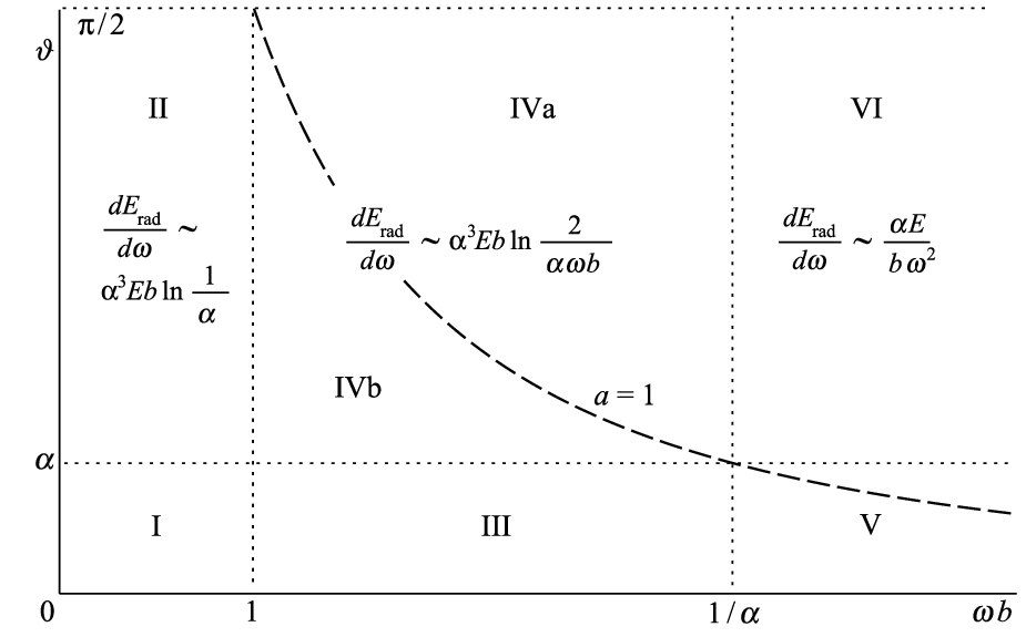
Refer to caption — Figure 1: The characteristic angular and frequency regimes.

4.1 Zero-frequency limit – Regimes I and II

In the low-frequency regime ( $\omega\to 0$ ) the amplitude $\tau_{\times}$ dominates and has the form

\displaystyle\tau_{\times}\simeq-\frac{16\sqrt{2}i{\kern 1.0pt}GE^{2}\,\sin\varphi}{\omega b\sin\vartheta}\,\!\!\int\limits_{0}^{1}dx\,{\rm e}^{-i(kb)x}\left[\hat{K}_{2}(\zeta)-\hat{K}_{1}(\zeta)\right],

(4.2)

while $\tau_{+}$ is finite and gives subleading contribution to (4.1). Note that in this limit ( $\hat{K}_{1}(0)=1$ , $\hat{K}_{2}(0)=2$ , ${\rm e}^{-i(kb)x}=1$ ) the $x-$ integration is trivial and gives $dE_{\rm rad}/d\omega=(2^{8}G^{3}E^{4}/\pi b^{{\kern 1.0pt}2})\int d\vartheta/\sin\vartheta$ , which diverges and implies that our formulae are not valid for $\vartheta$ close to zero.

We cannot trust our formulae in that regime and should repair them. A quick way to do it, is to impose a small-angle cut-off $\vartheta=\vartheta_{\rm cr}$ on the $\vartheta-$ integration, so as to obtain for $dE_{\rm rad}/d\omega|_{\omega=0}$ the value computed quantum mechanically in [5, 6], namely

\displaystyle\left(\frac{dE^{W}}{d\omega}\right)_{\!\omega=0}

\displaystyle=\frac{4}{\pi}\,G|t|\ln\frac{s}{|t|}=\frac{G\alpha^{2}s}{\pi}\,\ln\frac{4}{\alpha^{2}}=\frac{E{\kern 1.0pt}b}{\pi}\,\alpha^{3}\ln(2/\alpha)\,,\qquad s=4E^{2}\,,

(4.3)

which indeed agrees with our expression

\displaystyle\left(\frac{dE_{\rm rad}}{d\omega}\right)_{\!\omega=0}=\frac{2^{9}G^{3}E^{4}}{\pi b^{{\kern 1.0pt}2}}\int\limits_{\vartheta_{\rm cr}}^{\pi/2}\frac{d\vartheta}{\sin\vartheta}=\frac{E{\kern 1.0pt}b}{\pi}\,\alpha^{3}\,\ln\ctg\frac{\vartheta_{\rm cr}}{2}

(4.4)

for

\displaystyle\vartheta_{\rm cr}=\alpha\ll 1\,.

(4.5)

Thus, our result for the low frequency radiation emitted in a collision with large $s$ , fixed $t=-(s/2)\,(1-\cos\alpha)\simeq-s\alpha^{2}/4$ and $G|t|\leqslant{\mathcal{O}}(1)$ , agrees with the quantum computation of Weinberg, apart from a tiny emission angle $\vartheta\leqslant{\mathcal{O}}(\alpha)\ll 1$ in the forward direction ⁸⁸ 8 It should be pointed out that our classical computation reproduces the quantum results of Weinberg for soft graviton emission for $G|t|\ll{\mathcal{O}}(1)$ , i.e. for $(E/M_{\rm Pl})(r_{S}/b)\ll 1$ , or in Weinberg’s notation for $B\ll 1$ .. Furthermore, as will be shown next, at low frequencies $\omega$ and for $\vartheta\geqslant\alpha$ , the leading contribution to our classical amplitude, dominated in this regime by $T^{I\!I\!I}_{\mu\nu}$ (3.12), is identical to the one obtained in [6], after it is generalized (see below) to $b\neq 0$ ⁹⁹ 9 It is not surprising that the quantum and the classical results agree for the emitted energy of low frequency. As we argued, in the low-frequency regime, $dE_{\rm rad}/d\omega$ is dominated by the local source. The contribution of stress in this regime is negligible. As a result, the radiated gravitons are expected to be produced in a coherent state [12], and the corresponding expectation value of the quantum field to satisfy the classical field equations..

Indeed, following the notation of [6], we write for the energy-momentum source of the $2\to 2$ scattering process we are studying for arbitrary, a priori, scattering angle $\alpha$ and impact parameter $b$ :

		$\displaystyle\tilde{T}^{\mu\nu}({\bf x},t)=\sum_{n=1}^{2}\frac{P_{n}^{\mu}P_{n}^{\nu}}{E_{n}}\,\delta^{3}({\bf x}-{\bf v}_{n}t\mp{\bf b}/2)\,\theta(-t)+\sum_{n=1}^{2}\frac{\tilde{P}_{n}^{\mu}\tilde{P}_{n}^{\nu}}{\tilde{E}_{n}}\,\delta^{3}({\bf x}-\tilde{\bf v}_{n}t\mp{\bf b}/2)\,\theta(t)$
		$\displaystyle=\sum_{n=1}^{2}\frac{P_{n}^{\mu}P_{n}^{\nu}}{E_{n}}\,\delta^{3}({\bf x}-{\bf v}_{n}t\mp{\bf b}/2)+\sum_{n=1}^{2}\biggl(\frac{\tilde{P}_{n}^{\mu}\tilde{P}_{n}^{\nu}}{\tilde{E}_{n}}\,\delta^{3}({\bf x}-\tilde{\bf v}_{n}t\mp{\bf b}/2)-\frac{P_{n}^{\mu}P_{n}^{\nu}}{E_{n}}\,\delta^{3}({\bf x}-{\bf v}_{n}t\mp{\bf b}/2)\biggr)\theta(t)$

where $P_{n}^{\mu}(\tilde{P}_{n}^{\mu}),n=1,2$ , are the initial (final) particle momenta, with $\tilde{P}_{n}=\tilde{P}_{n}(P_{n},\alpha)$ . Its Fourier transform is

\displaystyle\tilde{T}^{\mu\nu}({\bf k},\omega)

\displaystyle=\sum_{n=1}^{2}2\pi{\rm e}^{\pm i(kb)/2}{P_{n}^{\mu}P_{n}^{\nu}}\,\delta(k\cdot P_{n})+\sum_{n=1}^{2}{\rm e}^{\pm i(kb)/2}\biggl(\frac{\tilde{P}_{n}^{\mu}\tilde{P}_{n}^{\nu}}{\tilde{E}_{n}}\frac{i}{\omega-{\bf k}\tilde{\bf v}_{n}}-\frac{P_{n}^{\mu}P_{n}^{\nu}}{E_{n}}\frac{i}{\omega-{\bf k}{\bf v}_{n}}\biggr),

where $k^{\mu}=(\omega,{\bf k})$ is the radiation wave-vector. The terms $n=1$ ( $n=2$ ) in the sums, are multiplied by ${\rm e}^{+i(kb)/2}$ $({\rm e}^{-i(kb)/2})$ , respectively.

The first sum, proportional to delta-functions, corresponds to no scattering and does not contribute to radiation. Thus, we end-up effectively with

\displaystyle\tilde{T}^{\mu\nu}_{\mathrm{eff}}(k)

\displaystyle=i\sum_{n=1}^{2}{\rm e}^{\pm i(kb)/2}\biggl(\frac{\tilde{P}_{n}^{\mu}\tilde{P}_{n}^{\nu}}{\tilde{E}_{n}}\frac{1}{\omega-{\bf k}\tilde{\bf v}_{n}}-\frac{P_{n}^{\mu}P_{n}^{\nu}}{E_{n}}\frac{1}{\omega-{\bf k}{\bf v}_{n}}\biggr).

(4.6)

To leading order in our approximation the scattering process, we are dealing with, is elastic with $\tilde{E}_{n}=E_{n}=E$ . Furthermore, write for the incoming particles $P_{n}^{\mu}=Eu_{n}^{\mu}=E(1,0,0,\pm 1)$ and for the outgoing ones $\tilde{P}_{n}^{\mu}=E\tilde{u}_{n}^{\mu}=E(u_{n}^{\mu}+\!\,^{1}\!\dot{z}_{n}^{\mu})=E(u_{n}^{\mu}\mp\alpha\,\hat{b}^{{\kern 1.0pt}\mu})\equiv P_{n}^{\mu}+\!\,^{1}\!P_{n}^{\mu}$ , substitute into $\tilde{T}_{\rm eff}^{\mu\nu}$ , and expand in powers of $\alpha$ using the fact that for $\vartheta>\alpha$ one has $|k\cdot\!\,^{1}\!P_{n}^{\mu}|\ll|k\cdot\!P_{n}^{\mu}|$ , to obtain

\displaystyle\tilde{T}^{\mu\nu}_{\mathrm{eff}}(k)=i\sum_{n=1}^{2}{\rm e}^{\pm i(kb)/2}\biggl(\frac{2P_{n}^{(\mu}\,{}^{1}\!P_{n}^{\nu)}}{(kP_{n})}-\frac{(k\,^{1}\!P_{n})}{(kP_{n})^{2}}\,P_{n}^{\mu}P_{n}^{\nu}\biggr)+\mathcal{O}(\alpha^{2})

(4.7)

or, finally, making use of the above definitions,

\displaystyle\tilde{T}^{\mu\nu}_{\mathrm{eff}}(k)=\frac{i\alpha E}{b}\sum_{n=1}^{2}\pm\,{\rm e}^{\pm i(kb)/2}\frac{(kb)\,u_{n}^{\mu}u_{n}^{\nu}-2(ku_{n})\,u_{n}^{(\mu}b^{\nu)}_{\vphantom{n}}}{(ku_{n})^{2}}=\frac{8iGE^{2}}{b^{{\kern 1.0pt}2}}\left[{\rm e}^{i(kb)/2}\frac{\sigma^{(u)}_{\mu\nu}}{(ku)^{2}}-{\rm e}^{-i(kb)/2}\frac{{\sigma}^{(u^{\prime})}_{\mu\nu}}{(ku^{\prime})^{2}}\right]\,.

(4.8)

This is identical to $T^{I\!I\!I}_{\mu\nu}$ in (3.12), after we bring the latter to its original form (3.6) by the substitution $\bar{\sigma}^{(u)}_{\mu\nu}\to\sigma^{(u^{\prime})}_{\mu\nu}$ . Q.E.D.

Summary: In regime II we use our formula, which is identical to Weinberg’s. We extend the use of Weinberg’s formula in regime I as well. The total emitted energy in I is known to be of $\,{\mathcal{O}}(\alpha^{3}E)$ . Given that $(dE_{\rm rad}/d\omega)_{\omega=0}\sim(dE_{\rm rad}/d\omega)_{\omega=1/b}$ , the contribution of II to the radiation efficiency is estimated by multiplying (4.4) by the frequency range $1/b$ and dividing by the initial energy $2E$ . The result is

\epsilon_{I,I{\kern-1.0pt}I}\sim\alpha^{3}\ln(1/\alpha)\,.

(4.9)

4.2 Regime VI

Here we consider the Regime VI ( $\omega>1/(\alpha b)=1/2r_{S}$ and $\vartheta>\alpha$ ). Contrary to regimes I and II, in regime VI as well as in IV, which will be discussed in the next subsection, the contributions to radiation of the local term and the stress are equally important.

The cross-amplitude (3.25) after an integration by parts of the second term reads:

\displaystyle\tau_{\times}(k)=-\frac{32i{\kern 1.0pt}Ge^{2}}{\sqrt{2}}\,\sin\varphi\left[\,\int\limits_{0}^{1}dx\,{\rm e}^{-i(kb)x}\!\left(\frac{\hat{K}_{2}(\zeta)\sin^{2}\!\varphi-\hat{K}_{1}(\zeta)}{a}\right)-\frac{4\cos\varphi}{a^{2}}\,{\rm e}^{-i(kb)/2}\sin\frac{kb}{2}\right]

with $a\equiv\omega b\sin\vartheta$ and together the two amplitudes are written as

		$\displaystyle\tau_{+}(k)=\frac{16{\kern 1.0pt}Ge^{2}}{\sqrt{2}}\,\left[-{L}_{0}+{L}_{1}\sin^{2}\!{\varphi}\,\vphantom{{c^{\prime}}^{M}}\right],$
		$\displaystyle\tau_{\times}(k)=-\frac{32i{\kern 1.0pt}Ge^{2}}{\sqrt{2}}\,\sin\varphi\,\left[\frac{L_{2}\sin^{2}\!\varphi-L_{1}}{a}-\frac{4\cos\varphi}{a^{2}}\,{\rm e}^{-i(kb)/2}\sin\frac{kb}{2}\right],$		(4.10)

where

L_{m}(a,\varphi)\equiv\int\limits_{0}^{1}{\rm e}^{iax\cos\varphi}\hat{K}_{m}\!\left(a\sqrt{x(1-x)}\right)dx

is defined and studied in Appendix C.

Substituting the large- $a$ expansion to leading order

L_{m}\simeq\frac{2^{m+2}\Gamma(m+1)}{a^{2}}\,\,{\rm e}^{ia\cos\varphi/2}\cos\frac{a\cos\varphi}{2}\,,

we obtain

\displaystyle\tau_{+}(k)\approx-\frac{64{\kern 1.0pt}Ge^{2}}{\sqrt{2}a^{2}}\,\cos 2{\varphi}\cos\frac{a\cos\varphi}{2}\,,\qquad\tau_{\times}(k)\approx-\frac{64i{\kern 1.0pt}Ge^{2}}{\sqrt{2}a^{2}}\,\sin 2\varphi\,\sin\frac{a\cos\varphi}{2}\,.

(4.11)

Thus

\displaystyle\frac{dE_{\rm rad}}{d\omega d\Omega}=\frac{2^{10}G^{3}E^{4}}{\pi^{2}}\frac{\omega^{2}}{a^{4}}\biggl[\cos^{2}\!2{\varphi}\cos^{2}\!\left(\frac{a\cos\varphi}{2}\right)+\sin^{2}\!2\varphi\sin^{2}\!\left(\frac{a\cos\varphi}{2}\right)\biggr].

(4.12)

Integrate over $\varphi$ using the formulae (A.7) to obtain for $a\gtrsim{\mathcal{O}}(1)$

\displaystyle\frac{dE_{\rm rad}}{d\omega d\vartheta}=\frac{2^{10}G^{3}E^{4}}{\pi}\frac{\omega^{2}}{a^{4}}\left[1-6\frac{J_{1}(a)}{a}-\left(1-\frac{24}{a^{2}}\right)J_{2}(a)\right]\sin\vartheta\sim\frac{2(\alpha b)^{3}E}{\pi}\,\frac{\omega^{2}}{a^{4}}\sin\vartheta\,,

(4.13)

from which one can obtain an estimate for the frequency distribution of the emitted radiation in regime VI by integrating over $\vartheta\in(\alpha,\pi-\alpha)$ , namely

\displaystyle\frac{dE^{V\!I}_{\rm rad}}{d\omega}\sim\frac{\alpha E}{b}\,\frac{1}{\omega^{2}}\,,\qquad\omega>1/\alpha b\,,

(4.14)

as well as an estimate for the emitted energy and the corresponding efficiency in regime VI, by integrating also over $\omega\in(1/\alpha b,\infty)$ ,

\displaystyle E^{V\!I}_{\rm rad}\sim\alpha^{2}E\qquad{\rm and}\qquad\epsilon_{V\!I}\sim\alpha^{2}.

(4.15)

4.3 Regimes II+IV+VI

Finally, we shall discuss the characteristics of the radiation corresponding to the union of regimes II+IV+VI. For that, it is convenient to transform the amplitudes (3.24) and (3.25) to the form

		$\displaystyle\tau_{+}(a,\varphi)=\frac{16{\kern 1.0pt}Gee^{\prime}}{\sqrt{2}}\,\int\limits_{0}^{1}dx\,{\rm e}^{iax\cos\varphi}\left[-{K}_{0}(\zeta)+\sin^{2}\!{\varphi}\,\hat{K}_{1}(\zeta)\right],$		(4.16)
		$\displaystyle\tau_{\times}(a,\varphi)=-\frac{16i{\kern 1.0pt}Gee^{\prime}}{\sqrt{2}}\,\sin\varphi\!\int\limits_{0}^{1}dx\,{\rm e}^{iax\cos\varphi}\!\left[2x{\kern 1.0pt}(1-x){\kern 1.0pt}a{\kern 1.0pt}{K}_{0}(\zeta)+\left(-i(2x-1)\cos\varphi+\frac{2}{a}\right)\!\hat{K}_{1}(\zeta)\right].$

Representing Macdonalds as

\displaystyle{K}_{0}(\zeta)=\int\limits_{0}^{\infty}\frac{\exp\left(-\zeta\sqrt{t^{2}+1}\right)}{\sqrt{t^{2}+1}}\,dt\,,\qquad\qquad\hat{K}_{1}(\zeta)=\zeta^{2}\int\limits_{0}^{\infty}\frac{\exp\left(-\zeta\sqrt{t^{2}+1}\right)}{\sqrt{t^{2}+1}}\,t^{2}\,dt\,,

(4.17)

we square and sum up the two polarizations:

		$\displaystyle\|\tau_{+}(a,\varphi)\|^{2}+\|\tau_{\times}(a,\varphi)\|^{2}=2^{7}{\kern 1.0pt}(Ge^{2})^{2}\,\int\limits_{0}^{1}dx\int\limits_{0}^{1}dx^{\prime}\int\limits_{0}^{\infty}dt\int\limits_{0}^{\infty}dt^{\prime}\,\frac{{\rm e}^{-a\Lambda(x,{\kern 1.0pt}t,{\kern 1.0pt}x^{\prime}\!,{\kern 1.0pt}t^{\prime}\!,{\kern 1.0pt}\varphi)}}{\sqrt{t^{2}+1}\sqrt{t^{\prime 2}+1}}\,\sum_{k=0}^{4}M_{k}(x,t,x^{\prime}\!,t^{\prime}\!,\varphi)\,a^{k},$
		$\displaystyle\Lambda(x,t,x^{\prime}\!,t^{\prime}\!,\varphi)=\sqrt{x(1-x)}\sqrt{t^{2}+1}+\sqrt{x^{\prime}(1-x^{\prime})}\sqrt{t^{\prime 2}+1}-i(x-x^{\prime})\cos\varphi$		(4.18)

with

		$\displaystyle M_{0}=1$
		$\displaystyle M_{1}=0$
		$\displaystyle M_{2}=x(1-x)\sin^{2}\!\varphi\left[-t^{2}+2x^{\prime}(1-x^{\prime})(1+2{\kern 1.0pt}t^{2}+t^{2}t^{\prime 2})\vphantom{{c^{\prime}}^{M}}\right]+\{x\longleftrightarrow x^{\prime},t\longleftrightarrow t^{\prime}\}$
		$\displaystyle M_{3}=2ixx^{\prime}(1-x)(1-x^{\prime})\,t^{\prime 2}\sin^{2}\!\varphi\cos\varphi\left[2x^{\prime}-1+2x^{\prime}t^{2}\vphantom{{c^{\prime}}^{M}}\right]-\{x\longleftrightarrow x^{\prime},t\longleftrightarrow t^{\prime}\}$
		$\displaystyle M_{4}=xx^{\prime}(1-x)(1-x^{\prime})\,t^{2}t^{\prime 2}\sin^{2}\!\varphi\left[\sin^{2}\!\varphi+(2x-1)(2x^{\prime}-1)\cos^{2}\!\varphi\vphantom{{c^{\prime}}^{M}}\right].$		(4.19)

One may substitute into (4.1) and integrate numerically over all variables apart from $\omega$ to obtain $dE_{\rm rad}/d\omega$ . The result is shown in Fig. 2. On the other hand, one may change variables and integrate over $a$ instead of $\omega$ to obtain:

\displaystyle\frac{dE_{\rm rad}}{d\vartheta}=\frac{2^{6}{\kern 1.0pt}G^{3}E^{4}}{\pi^{2}b^{{\kern 1.0pt}3}}\frac{1}{\sin^{2}\!\vartheta}\sum_{k=0}^{4}(k+2)!\int\limits_{0}^{1}dx\int\limits_{0}^{1}dx^{\prime}\int\limits_{0}^{\infty}\frac{dt}{\sqrt{t^{2}+1}}\int\limits_{0}^{\infty}\frac{dt^{\prime}}{\sqrt{t^{\prime 2}+1}}\int\limits_{0}^{2\pi}d\varphi\,\frac{M_{k}}{\Lambda^{k+3}}\,.

The convergence of this 5-variable integral follows from the behavior of the integrand at large- $a$ , while its numerical value is expected to be of $\mathcal{O}(1)$ , since the integrand does not contain any small or large parameter. Indeed, numerical integration (including the factorial in front) leads to

\displaystyle\eta\equiv\sum_{k=0}^{4}(k+2)!\int\limits_{0}^{1}dx\int\limits_{0}^{1}dx^{\prime}\int\limits_{0}^{\infty}dt\int\limits_{0}^{\infty}dt^{\prime}\int\limits_{0}^{2\pi}d\varphi\frac{M_{k}}{\Lambda^{k+3}\sqrt{t^{2}+1}\sqrt{t^{\prime 2}+1}}\approx 89.9\,.

(4.20)

Thus the angular distribution reads

\displaystyle\frac{dE_{\rm rad}}{d\vartheta}=\frac{\eta\alpha^{3}E}{8\pi^{2}}\frac{1}{\sin^{2}\!\vartheta}\,.

(4.21)

Integration over $\vartheta\in(\alpha,\pi-\alpha)$ gives

\displaystyle E_{\rm rad}=\frac{\eta{\kern 1.0pt}\alpha^{2}E}{4\pi^{2}}

(4.22)

and for the efficiency

\displaystyle\epsilon=\frac{E_{\rm rad}}{2E}\simeq 1.14\,\alpha^{2}\,.

(4.23)

Finally, the $\varphi-$ distribution of the emitted radiation is shown in Fig. 3, according to which most energy is emitted perpendicular to the scattering plane.

It is instructive to study regime IV in a little more detail. For that, let us split regime IV into IVa and IVb, as shown in Fig. 1, according to $a>1$ and $a<1$ , respectively. Inside the regime IVa the amplitude is damped as in regime VI. However, near the left border of regime IVb (with $1/b\lesssim\omega\ll 1/\alpha b$ ) one may expand the amplitudes in powers of $a$ and obtain, as in regime II:

\displaystyle\tau\simeq\tau_{\times}\simeq-\frac{16\sqrt{2}iGE^{2}}{\omega b}\frac{\sin\varphi}{\sin\vartheta}\,.

(4.24)

Upon integration over regime IVb, i.e. for $\alpha\lesssim\vartheta\lesssim\vartheta_{\rm max}=\arcsin(1/\omega b)$ one obtains

\displaystyle\left(\frac{dE_{\rm rad}}{d\omega}\right)_{\!1/b\lesssim\omega\ll 1/\alpha b}\simeq\frac{\alpha^{3}E{\kern 1.0pt}b}{\pi}\,\ln\frac{\tg(\vartheta_{\max}/2)}{\tg(\alpha/2)}\simeq\frac{\alpha^{3}E{\kern 1.0pt}b}{\pi}\,\ln\frac{2\alpha^{-1}}{\omega b+\sqrt{\omega^{2}b^{{\kern 1.0pt}2}-1}}\,.

Thus, for $1/b\lesssim\omega\ll 1/\alpha b$ one may approximate $dE_{\rm rad}/d\omega$ by

\left(\frac{dE_{\rm rad}}{d\omega}\right)_{\!1/b\lesssim\omega\ll 1/\alpha b}\simeq\frac{\alpha^{3}E{\kern 1.0pt}b}{\pi}\,\ln\frac{2}{\alpha\omega b}\,.

On the other hand, from the known behavior near $1/\alpha b\,$ from regime VI, we know that

\left(\frac{dE_{\rm rad}}{d\omega}\right)_{\omega\sim 1/\alpha b}\sim{\alpha^{3}E{\kern 1.0pt}b}\,.

So, a natural interpolation of $dE_{\rm rad}/d\omega$ between the values $1/b$ and $1/\alpha b$ is

\left(\frac{dE_{\rm rad}}{d\omega}\right)_{\!1/b\lesssim\omega\lesssim 1/\alpha b}=\frac{\alpha^{3}E{\kern 1.0pt}b}{\pi}\,\xi(\omega b)\,\ln\frac{2}{\alpha\omega b}\,.

(4.25)

It may be shown numerically that $\xi(\omega b)$ is a slowly varying function of ${\mathcal{O}}(1)$ in the regime $1/b\lesssim\omega\lesssim 1/\alpha b$ , so that one can simply write instead

\left(\frac{dE_{\rm rad}}{d\omega}\right)_{\!1/b\lesssim\omega\lesssim 1/\alpha b}\sim\alpha^{3}E{\kern 1.0pt}b\,\ln\frac{2}{\alpha\omega b}\,.

(4.26)

It should be pointed out here that the integral of $dE_{\rm rad}/d\omega$ over $\omega$ receives most of its contribution from frequencies in the neighborhood of $1/\alpha b$ in both regimes IV and VI. Thus, one can say that the characteristic frequency of the emitted radiation is around ${\mathcal{O}}(1/r_{S})$ .

4.4 Comparison to previous work

Let us briefly compare the results of the present paper with our previous calculation of massive particle collisions and to the previous literature as well. In relation to our work, we should point out that it is not straightforward to compare with [1], simply because they are were based on different assumptions and approximations. In particular, in the massive case we worked in the lab-frame and assumed weak-field approximation, restricting $\gamma_{\rm cm}$ to $\gamma_{\rm cm}\ll 1/\alpha$ , which is not consistent for fixed $\alpha$ with the $\gamma_{\rm cm}\to\infty$ limit, necessary to connect with the massless case. On the other hand, in the massless case the computation is characterized by $\gamma_{\rm cm}=\infty$ , is performed in the center-of-mass frame, used the scattering angle $\alpha$ as an angular integration cut-off, and used Weinberg’s results in regime I. So, before it is appropriate to compare with the massive case, we have to redo the latter following the same methodology and approximations. This, as well as comparison with other papers in the literature is the content of this subsection.

In [1] we computed the gravitational radiation efficiency in ultra relativistic massive particle collisions in $D$ dimensions and in the weak field limit, i.e. for $1\ll\gamma_{\rm cm}\ll 1/\alpha$ . Specifically, in $D=4$ we obtained $\epsilon\sim\alpha^{3}\gamma_{\rm cm}$ , with the emitted radiation having characteristic frequency $\omega_{\rm cm}\sim\gamma_{\rm cm}/b$ and emission angle $\vartheta\sim 1/\gamma_{\rm cm}$ , where $b$ is the impact parameter. Thus, the efficiency is finite in the above kinematical regime and agrees with the results of [15] and [16].

However, to compare with the massless case we have to improve the massive case computation in two ways: (i) discard the weak-field condition as it is done here and more generally in the literature, e.g. [3, 10, 11], and (ii) use the scattering angle $\alpha$ as a characteristic angle to cut-off angular integrations. As a consequence of (i) the condition $1\ll\gamma_{\rm cm}\ll 1/\alpha$ is replaced by $\gamma_{\rm cm}\gg 1$ and $1/\alpha\gg 1$ , independently; so that for $\gamma_{\rm cm}\to\infty$ one would naively conclude that $\epsilon\sim\alpha^{3}\gamma_{\rm cm}\to\infty$ , in disagreement with the present massless result $\epsilon\sim\alpha^{2}$ . But, as we will argue next, the formula $\epsilon\sim\alpha^{3}\gamma_{\rm cm}$ is not valid in this case and the present result from regimes I-IV and VI, defined by $\alpha$ , $1/b$ and $1/\alpha b$ as in Fig. 1, is actually in agreement with the limit $\gamma_{\rm cm}\to\infty$ of the contribution from those regimes in the massive case.

Let us start with regime ${\rm IV_{a}+VI}$ . Due to destructive interference [1], the total radiation amplitude is

\displaystyle\tau(\omega,\vartheta)\sim\frac{Gm^{2}\gamma^{2}_{\rm cm}}{(\omega b\sin\vartheta)^{2}}\,,

(4.27)

which upon integration over this region gives $\epsilon\sim\alpha^{2}+{\mathcal{O}}{\kern 1.0pt}(1/\gamma_{\rm cm})$ .

The contribution from regimes ${\rm II+IV_{b}}$ can be computed as in the massless case. That is, starting with the observation that in that regime the direct amplitude $T$ dominates over the stress $S$ , we take for $T$ the expression [1, Eqn. (3.17)]¹⁰¹⁰ 10 In this expression the true 4-velocity $U^{\mu}$ normalized by $U^{2}=1$ , is defined as $U^{\mu}=\gamma_{\rm cm}u^{\mu}$ with $u^{\mu}_{1,2}=(1,0,0,\pm v_{\rm cm})$ and $v_{\rm cm}^{2}=1-\gamma_{\rm cm}^{-2}$ .

\,{}^{1}\!T^{\mu\nu}(k)\sim\frac{i{\kern 1.0pt}Gm^{2}\gamma_{\rm cm}^{2}}{b^{2}}\sum_{n=1}^{2}\pm\,{\rm e}^{\pm i(kb)/2}\frac{(kb)\,u_{n}^{\mu}u_{n}^{\nu}-2(ku_{n})\,u_{n}^{(\mu}b^{\nu)}_{\vphantom{n}}}{(ku_{n})^{2}}\,\hat{K}_{1}\!\left(\frac{(ku_{n}){\kern 1.0pt}b}{2\gamma_{\rm cm}}\right)

(4.28)

and integrate over the above regime to obtain again $\epsilon\sim\alpha^{2}$ , plus subleading corrections of order $1/\gamma_{\rm cm}$ .

Next, one can, following the approach discussed in subsection 4.1 above, use instead of (4.28) the expression $\tilde{T}^{\mu\nu}_{\rm eff}$ given in (4.6), valid for both massive and massless colliding particles. This allows us to integrate over all angles and upon integration over I+III to obtain again to $\epsilon\sim\alpha^{2}$ . Furthermore, this approach eliminates the disagreement of [1, Eqn. (4.15)] as well as of Smarr [14, Eqn. (2.13)] in the expression for $dE_{\rm rad}/d\omega$ in the zero frequency limit with the corresponding result of Weinberg. Specifically, the non-sensical for $\gamma_{\rm cm}\to\infty$ formula $(dE_{\rm rad}/d\omega)_{\omega=0}\simeq(Gs\alpha^{2}/\pi)\ln(4\gamma^{2}_{\rm cm})$ gets modified to $(dE_{\rm rad}/d\omega)_{\omega=0}\simeq(Gs\alpha^{2}/\pi)\ln(s/|t|)$ given in (4.3).

Finally, in regime V the direct amplitude and the stress are equally important, both for massive as well as massless colliding particles. This was important in deriving destructive interference, but on the other hand it does not allow us to replace the source amplitude with Weinberg’s formula for $T$ . To proceed along these lines, one has to “guess” the correct corresponding modification of $S$ , consistent with the conservation requirements for the total energy momentum tensor. This problem is currently under investigation.

Thus, indeed, the results of the present paper can be obtained as the massless limit of the corresponding conclusions of the massive case in their common region of validity.

5 Conclusions – Discussion

Using the same approach as in [1], based on standard GR, with the leading non-linear gravity effects taken into account, we studied collisions of massless particles and computed the gravitational energy of arbitrary frequency, which is emitted outside the cone of angle $\alpha=2r_{S}/b\ll 1$ in the forward and backward directions. The value $\epsilon\simeq 1.14\,\alpha^{2}$ was obtained for the radiation efficiency, with characteristic frequency $\omega\sim 1/r_{S}$ . In fact, this value represents a lower bound of the efficiency, since it does not include the energy emitted inside that cone. The frequency distribution of radiation in the characteristic angle-frequency regimes is shown in Fig. 1. Our method allowed to study the zero frequency regime and showed that the values $dE_{\rm rad}/d\omega$ at $\omega=0$ and $1/b$ are of the same order.

We would like to point out that our results about regime IV agree with Gruzinov and Veneziano [10]. Furthermore, our work provides information about the very low frequency regime II, in which, strictly speaking, the method of [10] cannot be applied. Finally, at frequencies $\omega\lesssim 1/\alpha b$ we obtain $\epsilon\sim\alpha^{2}$ , i.e. the same dependence as in [10]. A possible difference in the coefficients is expected, since the non-linear stress contribution around $\omega\sim 1/\alpha b$ is comparable to the contribution of the direct linearized emission from the colliding particles. However, as mentioned several times, our approach cannot yet deal reliably with regime V, which according to [10] gives dominant contribution in $\epsilon$ by an extra factor $\ln 1/\alpha$ . In particular, we cannot yet confirm the presence of any other characteristic frequency, such as e.g. $1/\alpha^{3}b$ , or characteristic emission angle smaller than $\alpha$ [10]. We hope to return to these issues with a better understanding of regime V in the near future.

Acknowledgments. We would like to acknowledge enlightening discussions with D. Gal’tsov, G. Veneziano, A. Gruzinov and S. Dubovsky. This work was supported in part by the EU program “Thales” (MIS 375734) and was also co-financed by the European Union (European Social Fund, ESF) and Greek national funds under the “ARISTEIA II” Action. TNT would like to thank the Theory Unit of CERN for its hospitality during the later stages of this work. PS is grateful for financial support from the RFBR under grant 14-02-01092, as well as from the non-commercial “Dynasty” Foundation (Russian Federation).

Appendix A Conventions

Our convention for the Minkowski metric is $\eta_{\mu\nu}=\eta^{{\kern 1.0pt}\mu\nu}={\rm diag}(+1,-1,-1,-1)$ .

Fourier transforms are defined as:

\displaystyle f(x)=\frac{1}{(2\pi)^{4}}\int f(k)\,{\rm e}^{-i(kx)}d^{{\kern 1.0pt}4}k\,,\qquad f(k)=\int f(x)\,{\rm e}^{i(kx)}d^{{\kern 1.0pt}4}x\equiv\mathcal{F}[f(x)](k)\,.

(A.1)

We use the following symmetrization notation for tensorial indices: $a_{(\mu}b_{\nu)}=[\vphantom{{c}^{M}}a_{\mu}b_{\nu}+a_{\nu}b_{\mu}]/2$ .

Polarization tensors. Given the radiation null wave-vector $k^{\mu}$ and the null velocities $u^{\mu}$ and $u^{\prime\mu}$ , define the polarization vectors $e_{1}$ and $e_{2}$ by:

e_{1}^{\mu}=\frac{1}{k_{\bot}}\left[\frac{(ku){\kern 1.0pt}u^{\prime\mu}-(ku^{\prime}){\kern 1.0pt}u^{\mu}}{2}-\frac{ku-ku^{\prime}}{ku+ku^{\prime}}\,k^{\mu}\right],\qquad e_{2}^{\mu}=\frac{1}{2k_{\bot}}\,\epsilon^{{\kern 1.0pt}\mu\nu\lambda\rho}u_{\nu}u^{\prime}_{\lambda}k_{\rho}\,,

(A.2)

where $k_{\bot}^{2}=(ku)(ku^{\prime})$ and $\epsilon^{0123}=1$ . They satisfy

e_{1}\cdot e_{2}=k\cdot e_{1}=k\cdot e_{2}=0\qquad{\rm and}\qquad e_{2}\cdot u=e_{2}\cdot u^{\prime}=e_{2}\cdot k=0\,.

(A.3)

In the center of mass frame of the collision under study we have chosen $u^{\mu}=(1,0,0,1)$ , $u^{\prime\mu}=(1,0,0,-1)$ and $b^{{\kern 1.0pt}\mu}=(0,b,0,0)$ . In addition, we have defined $k^{\mu}=\omega(1,{\bf n})\equiv\omega(1,\sin\vartheta\cos\varphi,\sin\vartheta\sin\varphi,\cos\vartheta)$ . Using these, we obtain

e_{1}^{\mu}=(0,\partial{\bf n}/\partial\vartheta)\,,\qquad e_{2}^{\mu}=\frac{1}{\sin\vartheta}\,(0,\partial{\bf n}/\partial\varphi)

(A.4)

and

e_{1}\cdot u=\sin\vartheta\,,\qquad e_{1}\cdot u^{\prime}=-\sin\vartheta\,,\qquad e_{1}\cdot b=-b{\kern 1.0pt}\cos\vartheta\,\cos\varphi\,,\qquad e_{2}\cdot b=-b\sin\varphi\,.

(A.5)

Finally, using $e_{1}$ and $e_{2}$ , we define the polarization tensors as

{\varepsilon}_{+}^{\mu\nu}=\frac{e_{1}^{\mu}e_{1}^{{\vphantom{\mu}}\nu}-e_{2}^{\mu}e_{2}^{{\vphantom{\mu}}\nu}}{\sqrt{2}}\,,\qquad{\varepsilon}_{\times}^{\mu\nu}=\sqrt{2}\,e_{1}^{(\mu}e_{2}^{\nu)}\,,\qquad{\varepsilon}_{{\cal{P}}}^{\mu\nu}\eta_{\mu\nu}=0\,,\qquad{\cal{P}}=+,\times\,.

(A.6)

Useful integrals. The following integrals are used in the main text:

		$\displaystyle\int\limits_{0}^{2\pi}\sin^{2}\!\varphi\sin^{2}\!\left(\frac{a\cos\varphi}{2}\right)\,d\varphi=\pi\left(\frac{1}{2}-\frac{J_{1}(a)}{a}\right),$		$\displaystyle\int\limits_{0}^{2\pi}\cos^{2}\!\varphi\sin^{2}\!\left(\frac{a\cos\varphi}{2}\right)\,d\varphi=\pi\left(\frac{1}{2}-J_{0}(a)+\frac{J_{1}(a)}{a}\right),$
		$\displaystyle\int\limits_{0}^{2\pi}\sin^{4}\!\varphi\sin^{2}\!\left(\frac{a\cos\varphi}{2}\right)\,d\varphi=3\pi\left(\frac{1}{8}-\frac{J_{2}(a)}{a^{2}}\right)\,,$		$\displaystyle\int\limits_{0}^{2\pi}\cos^{4}\!\varphi\sin^{2}\!\left(\frac{a\cos\varphi}{2}\right)\,d\varphi=\pi\left[\frac{3}{8}+\left(1-\frac{3}{a^{2}}\right)J_{2}(a)\right].$		(A.7)

Appendix B Computation of momentum integrals

It is convenient for the computation of the integrals below to define the four vector $b^{{\kern 1.0pt}\mu}$ by:

b^{{\kern 1.0pt}\mu}\equiv\frac{1}{2}\left[\vphantom{{c^{\prime}}^{M}}(bu)\,u^{\prime\mu}+(bu^{\prime})\,u^{\mu}\right]+b_{\perp}^{{\kern 1.0pt}\mu}.

Local integrals. The basic scalar integral is

\displaystyle I=\frac{1}{(2\pi)^{2}}\int\frac{\delta(qu^{\prime})\,\delta(ku-qu)\,{\rm e}^{-i(qb)}}{q^{2}}\;d^{{\kern 1.0pt}4}{\kern-1.0pt}q=-\frac{{\rm e}^{-i(bu^{\prime})(ku)/2}}{2{\kern 1.0pt}(2\pi)^{2}}\int\frac{{\rm e}^{i\mathbf{qb}}}{\mathbf{q}^{2}}\,d^{{\kern 1.0pt}2}\mathbf{q}=-{{\rm e}^{-i(bu^{\prime})(ku)/2}}\frac{\Phi(b)}{2}\

(B.1)

with $b\equiv\sqrt{-b\cdot b}$ and $\Phi(r)\equiv-(1/2\pi)\ln(r/r_{0})$ .

The local vector momentum integral is defined as

\displaystyle I_{\mu}\equiv\frac{1}{(2\pi)^{2}}\int\frac{\delta(qu^{\prime})\,\delta(ku-qu)\,{\rm e}^{-i(qb)}}{q^{2}}\;q_{\mu}\;d^{{\kern 1.0pt}4}{\kern-1.0pt}q=i\frac{\partial I}{\partial b^{{\kern 1.0pt}\mu}}=-{\rm e}^{-i(bu^{\prime})(ku)/2}\left[\frac{(ku)\,\Phi(b)}{4}\,u^{\prime}_{\mu}-i\frac{\Phi^{\prime}(b)}{2b}\,b_{\mu}\right].

(B.2)

The corresponding integrals for the primed particle are obtained by the substitution $u^{\mu}\leftrightarrow u^{\prime\mu},b^{{\kern 1.0pt}\mu}\to-b^{{\kern 1.0pt}\mu}$ .

Stress integrals. The covariant stress integrals are defined by

\displaystyle J\equiv\frac{1}{(2\pi)^{2}}\int\frac{\delta(qu^{\prime})\,\delta(ku-qu)\,{\rm e}^{-i(qb)}}{q^{2}(k-q)^{2}}\;d^{{\kern 1.0pt}4}{\kern-1.0pt}q\,,\qquad J_{\mu}\equiv i\frac{\partial J}{\partial b^{{\kern 1.0pt}\mu}}\,,\qquad J_{\mu\nu}\equiv-\frac{\partial^{2}J}{\partial b^{{\kern 1.0pt}\mu}\partial b^{\nu}}\,.

(B.3)

$\bullet$ We start with the computation of $J$ . We will then compute the other stress integrals as derivatives of $J$ , following the same procedure as above, but to avoid unnecessary complications we will give the final expressions only for the special choice $b^{{\kern 1.0pt}\mu}=(0,1,0,0)$ made in the main text. We obtain ¹¹¹¹ 11 Use was made of the formulae $\int\limits_{0}^{\pi}e^{\pm iz\cos\theta}\sin^{2k}\theta d\theta=\frac{2^{k}\Gamma(k+1/2)\sqrt{\pi}}{z^{k}}J_{k}(z)\,,\qquad\int\limits_{0}^{\infty}dy\frac{y^{n+1}J_{n}(by)}{[y^{2}+a^{2}]^{m}}=\frac{b^{{\kern 1.0pt}m-1}|a|^{n-m+1}}{2^{m-1}\Gamma(m)}\,K_{n-m+1}(b\hskip 1.49994pt|a|)\,.$

	$\displaystyle J$	$\displaystyle=\frac{1}{8\pi^{2}}\int\frac{{\rm e}^{i\mathbf{q}\mathbf{b}}}{\mathbf{q}^{2}(\mathbf{k}-\mathbf{q})^{2}}\;d^{{\kern 1.0pt}2}\mathbf{q}=\frac{1}{2\pi^{2}}\int\limits_{0}^{1}dx\;{\rm e}^{-i(kb)x}\int\limits_{0}^{\pi}d\theta\int\limits_{0}^{\infty}dq\frac{{\rm e}^{iqb\cos\theta}}{[{\mathbf{q}}^{2}+\mathbf{k}^{2}x(1-x)]^{2}}\,q=$
		$\displaystyle=\frac{1}{4\pi}\int\limits_{0}^{1}dx\;{\rm e}^{-i(kb)x}\int\limits_{0}^{\infty}d{q}\,\frac{q\,J_{0}(qb)}{[{\mathbf{q}}^{2}+\mathbf{k}^{2}x(1-x)]^{2}}=\frac{b^{{\kern 1.0pt}2}}{8\pi}\int\limits_{0}^{1}dx\,{\rm e}^{-i(kb)x}\hat{K}_{-1}\!\left(k_{\perp}b\sqrt{x(1-x)}\right),$

where $k_{\perp}\equiv|{\bf k}|=\sqrt{(ku)(ku^{\prime})}$ is the magnitude of the two-dimensional transverse part of $k^{{\kern 1.0pt}\mu}$ .

Also ¹²¹² 12 A useful formula is $\displaystyle J^{0}=-J^{z}=\frac{(ku)}{2}\,J\,.$ ,

\displaystyle J_{\mu}=\frac{b^{{\kern 1.0pt}2}}{8\pi}\int\limits_{0}^{1}dx\;{\rm e}^{-i(kb)x}\left[N_{\mu}\hat{K}_{-1}\!\left(\zeta\right)+i\frac{b_{\mu}}{b^{{\kern 1.0pt}2}}\,{K}_{0}\!\left(\zeta\right)\right]\,,\;\;\;\;\;\;N^{\mu}\equiv xk^{{\kern 1.0pt}\mu}-\frac{1}{2}\left[x(ku^{\prime})\,u^{\mu}-(1-x)(ku)\,{u^{\prime}}^{\mu}\vphantom{{c^{\prime}}^{M}}\right],

(B.4)

where $\zeta\equiv k_{\perp}b\sqrt{x(1-x)}$ .

$\bullet$ Next consider $(kJ)$ . With the on-shell condition $k^{2}=0\,$ it can be represented as

	$\displaystyle k\cdot J$	$\displaystyle=\int\frac{\delta(qu^{\prime})\,\delta(ku-qu)\,{\rm e}^{-i(qb)}}{q^{2}(k-q)^{2}}\;(kq)\;d^{{\kern 1.0pt}4}{\kern-1.0pt}q=\frac{1}{2}\int\frac{\delta(qu^{\prime})\,\delta(ku-qu)\,{\rm e}^{-i(qb)}}{q^{2}(k-q)^{2}}\,\left[q^{2}-(k-q)^{2}\right]\,d^{{\kern 1.0pt}4}{\kern-1.0pt}q=$
		$\displaystyle=\frac{1}{2}\left[{\rm e}^{-i(kb)}I^{*}-I\right]=\frac{I}{2}\left[{\rm e}^{-i(kb)}-1\right]=\frac{\Phi(b)}{4}\left[1-{\rm e}^{-i(kb)}\right].$		(B.5)

On the other hand, the integral form (B.4) of $J_{\mu}$ becomes

\displaystyle k\cdot J=\frac{1}{8\pi}\int\limits_{0}^{1}dx\;{\rm e}^{-i(kb)x}\left[\left(\frac{1}{2}-x\right){k}_{\perp}^{2}b^{{\kern 1.0pt}2}\hat{K}_{-1}\!\left(k_{\perp}b\sqrt{x(1-x)}\right)+i(kb)\,{K}_{0}\!\left(k_{\perp}b\sqrt{x(1-x)}\right)\right],

whose integrand is the derivative of $-{\rm e}^{-i(kb)x}{K}_{0}\!\left(k_{\perp}b\sqrt{x(1-x)}\right)$ . Hence,

\displaystyle k\cdot J=\frac{1}{8\pi}\left.{\rm e}^{-i(kb)x}\hat{K}_{0}\!\left(k_{\perp}b\sqrt{x(1-x)}\right)\right|_{1}^{0}=\lim_{d\to+0}\frac{\hat{K}_{d/2}(0)}{8\pi}\left[1-{\rm e}^{-i(kb)}\right]=\frac{\Phi(b)}{4}\left[1-{\rm e}^{-i(kb)}\right].

(B.6)

$\bullet$ Following similar steps, we find for the tensorial integral

\displaystyle J_{\mu\nu}=\frac{1}{8\pi}\int\limits_{0}^{1}dx\;{\rm e}^{-i(kb)x}

\displaystyle\left[b^{{\kern 1.0pt}2}N_{\mu}N_{\nu}\hat{K}_{-1}(\zeta)+\left(2iN_{(\mu}b_{\nu)}-\eta_{\mu\nu}+u^{\vphantom{\prime}}_{(\mu}u^{\prime}_{\nu)}\right){K}_{0}(\zeta)-\frac{b_{\mu}b_{\nu}}{b^{{\kern 1.0pt}2}}\,\hat{K}_{1}(\zeta)\right].

(B.7)

$\bullet$ Its trace $\Sp J\equiv\eta^{{\kern 1.0pt}\mu\nu}J_{\mu\nu}$ is given by

\displaystyle\Sp J=\frac{1}{8\pi}\int\limits_{0}^{1}dx\;{\rm e}^{-i(kb)x}

\displaystyle\left[-x^{2}b^{{\kern 1.0pt}2}k_{\perp}^{2}\hat{K}_{-1}(\zeta)+2ix(kb){K}_{0}(\zeta)+\hat{K}_{1}(\zeta)-2{K}_{0}(\zeta)\right].

Make use of the Macdonald-function identity $\hat{K}_{1}(z)=z^{2}\hat{K}_{-1}(z)$ to obtain

\displaystyle\Sp J=\frac{1}{8\pi}\int\limits_{0}^{1}dx\;{\rm e}^{-i(kb)x}

\displaystyle\left[-x(2x-1)\,b^{{\kern 1.0pt}2}k_{\perp}^{2}\hat{K}_{-1}(\zeta)+2\left(\vphantom{{c^{\prime}}^{M}}ix(kb)-1\right)\!{K}_{0}(\zeta)\right].

The integrand is the total derivative of $-2x\,{\rm e}^{-i(kb)x}{K}_{0}\!\left(k_{\perp}b\sqrt{x(1-x)}\right)$ . Hence

\displaystyle\Sp J=\frac{x}{4\pi}\left.{\rm e}^{-i(kb)x}{K}_{0}\!\left(k_{\perp}b\sqrt{x(1-x)}\right)\right|_{1}^{0}=-{\rm e}^{-i(kb)}\frac{\Phi(b)}{2}={\rm e}^{-i(kb)}I\,.

(B.8)

Appendix C Asymptotic expansion of higher-frequency integrals

We are interested here in the expansion of the typical integrals

L_{m}\equiv\int\limits_{0}^{1}{\rm e}^{-icx}\hat{K}_{m}\!\left(a\sqrt{x(1-x)}\right)dx

(where $c=k\cdot b=-a\cos\varphi$ ) in powers of $1/a$ for $a\gg 1$ . The presence of the $\sqrt{x(1-x)}$ in the argument of the $K_{m}$ , prevents the direct use of an asymptotic expansion of the Macdonald function itself. Instead, we shall proceed as follows: we represent

L_{m}=\sqrt{\frac{2}{\pi}}\,\left(\frac{a}{2}\right)^{2m+1}\int\limits_{0}^{\infty}dy\check{K}_{m+1/2}\!\left(\frac{a}{2}\sqrt{y^{2}+1}\right)\int\limits_{0}^{1}{\rm e}^{-icx}\ch\!\left(\vphantom{{c^{\prime}}^{M}}ay\left(x-{1}/{2}\right)\right)dx\,,

where $\check{K}_{m}(z)\equiv z^{-m}K_{m}(z)$ . Making use of

\int\limits_{0}^{1}{\rm e}^{-icx}\ch\!\left(\vphantom{{c^{\prime}}^{M}}s\left(x-{1}/{2}\right)\right)dx=\frac{2{\kern 1.0pt}{\rm e}^{-ic/2}}{s^{2}+c^{2}}\left[s\sh\frac{s}{2}\cos\frac{c}{2}+c\ch\frac{s}{2}\sin\frac{|c|}{2}\right],\qquad s^{2}\geqslant c^{2},

one obtains

\displaystyle L_{m}=\frac{2{\kern 1.0pt}{\rm e}^{-ic/2}}{a^{2}}\sqrt{\frac{2}{\pi}}\,\left(\frac{a}{2}\right)^{2m+1}\int\limits_{0}^{\infty}dy\,\frac{\check{K}_{m+1/2}\!\left(\displaystyle\frac{a}{2}\sqrt{y^{2}+1}\right)}{y^{2}+\cos^{2}\!\varphi}\left[ay\sh\frac{ay}{2}\cos\frac{c}{2}+c\ch\frac{ay}{2}\sin\frac{|c|}{2}\right].

(C.1)

Then one may use the expansion

\frac{1}{y^{2}+\cos^{2}\!\varphi}=\sum_{k=0}^{\infty}\frac{\sin^{2k}\!\varphi}{(y^{2}+1)^{k+1}}\,,

which converges since $y^{2}+1\geqslant 1$ , $\sin^{2}\!\varphi\leqslant 1$ ¹³¹³ 13 Notice, that the series is convergent even for the limiting value $\cos\varphi=0$ , while the integral (C.1) converges for $y\to 0$ , as a consequence of $\lim_{y\to 0}\frac{\sh(ay/2)}{y}=\frac{a}{2}\,,\qquad\lim_{c\to 0}\frac{c\sin(|c|/2)}{y^{2}+c^{2}/a^{2}}=\frac{a^{2}}{2}\,.$ .

The next step is to integrate over $y$ using the formulae ( $q\geqslant|r|$ )

\displaystyle q^{2\nu}\int\limits_{0}^{\infty}\!dy\,\check{K}_{\nu}\!\left(q\sqrt{y^{2}+1}\right)\left\{\begin{array}[]{c}y\sh(ry)\\ \ch(ry)\\ \end{array}\right\}=\sqrt{\frac{\pi}{2}}\left\{\begin{array}[]{c}r\hat{K}_{\nu-3/2}(\sqrt{q^{2}-r^{2}})\\ \hat{K}_{\nu-1/2}(\sqrt{q^{2}-r^{2}})\\ \end{array}\right\}

together with the identity

\displaystyle K_{\nu}(z)=K_{\nu+2}(z)-\frac{2(\nu+1)}{z}\,K_{\nu+1}(z)\simeq K_{\nu+2}(z)\,,\quad{\rm for}\;\;z\gg 1\,.

(C.6)

Explicitly, applying (C.6) once, the leading term is the one containing $\sh(ay/2)$ and is given by:

\frac{2{\kern 1.0pt}}{a}\sqrt{\frac{2}{\pi}}\,\left(\frac{a}{2}\right)^{2m+3}\int\limits_{0}^{\infty}dy\,\check{K}_{m+5/2}\!\left(\frac{a}{2}\sqrt{y^{2}+1}\right)y\sh\frac{ay}{2}\cos\frac{c}{2}=\frac{2^{m+2}\Gamma(m+1)}{a^{2}}\,\cos\frac{c}{2}\,.

The first subleading term is $\mathcal{O}{\kern 1.0pt}(a^{-3})$ : it comes from $\ch(ay/2)$ times basic Macdonald; the next subleading terms are $\mathcal{O}{\kern 1.0pt}(a^{-4})$ : they come (i) from $y\sh(ay/2)$ times previous shift-index term; and (ii) $y\sh(ay/2)$ times first correction in $\sin^{2}\!\varphi$ . The end result is:

L_{m}=\frac{2^{m+2}\Gamma(m+1)}{a^{2}}\,{\rm e}^{-ic/2}\cos\frac{c}{2}\left[1-\frac{m+1}{a^{2}}\left(4{\kern 1.0pt}a\cos\varphi\,\tg\frac{c}{2}+8{\kern 1.0pt}(2m+3)-16(m+2)\,\sin^{2}\!\varphi\right)+\mathcal{O}\Bigl(\frac{1}{a^{3}}\Bigr)\right].

References

[1] D. Gal’tsov, P. Spirin and T. N. Tomaras , JHEP01 (2013) 087, arXiv:1210.6976 [hep-th].
[2] D. V. Gal’tsov, G. Kofinas, P. Spirin and T. N. Tomaras , Phys. Lett. B683 (2010) 331, arXiv:0908.0675 [hep-ph].
[3] V. Ferrari, P. Pendenza and G. Veneziano, Gen. Rel. Grav. 20, 1185 (1988).
[4] G. Dvali, C. Gomez, R. S. Isermann, D. Lüst and S. Stieberger, Nucl. Phys. B893 (2015) 187-235, arXiv:1409.7405 [hep-th].
[5] S. Weinberg, Phys. Rev. 140 (1965) B516.
[6] S. Weinberg, “Gravitation and Cosmology”, Chapter 10; J. Wiley and Sons, 1972.
[7] P. D. D’Eath and P. N. Payne, Phys. Rev. D46, 658, 675, 694 (1992).
[8] C. Herdeiro, M. O. P. Sampaio and C. Rebelo, JHEP 1107 (2011) 121, arXiv:1105.2298 [hep-th].
[9] Y. Constantinou and A. Taliotis, JHEP 1311 (2013) 175, arXiv: 1308.2544 [hep-th].
[10] A. Gruzinov and G. Veneziano, arXiv:1409.4555v1 [gr-qc].
[11] T. Dray and G. ’t Hooft, Nucl. Phys. B253 (1985) 173.
[12] R. Glauber, “Quantum Theory of Optical Coherence”, chapter 2; J. Wiley, 2007.
[13] I. M. Gel’fand and G. E. Shilov, “Generalized Functions: Properties and operations”, Academic Press, Waltham, MA, 1964.
[14] L. Smarr, Phys. Rev. D15, 2069 (1977).
[15] P. C. Peters, Phys. Rev. D1, 1559 (1970).
[16] S. J. Kovacs and K. S. Thorne, Astrophys. J. 224, 62 (1978).