Matrix product state approach to a frustrated spin chain with long-range interactions
Abstract
We make extensive simulations over a spin chain model that combines the frustrated spin chain and the long-range nonfrustrated decay interactions through the variational matrix product state method for both finite and infinite lengths. We study both the ground state entanglement and phase diagram. We find that it is most entangled in the rotation invariant long-range ordered antiferromagnetic phase, where the entanglement scales approximately logarithmically. We determine the development of the Majudar-Ghosh point to a disorder line from entanglement. And we determine approximately the transition from the dimerized and incommensurate phase of the model to a decoupled phase by studying spin correlation and the dimerization order parameter. Some implications for entanglement in systems with long-range interactions are stated.
I introduction
Quantum spin chains are the fertile ground to study strongly correlated quantum many body effects. One of the most studied models is the quantum Heisenberg model. For antiferromagnetic coupling () the spin correlation of its ground state decays as up to a logarithm correction [1, *giamarchi1989correlation] displaying quasi-long range order (QLRO). The model with a next-nearest neighbour added is known as the or zigzag spin chain. It is frustrated when . A dimerization transition occurs at after which it has a valence-bond-solid (VBS) order [3, 4] and incommensurate spiral spin correlation emerges after the Majudar-Ghosh (MG) point at [5, 6, 7].
Beyond the next-nearest terms, the system can be built up with even long-range interactions (LRI). The models with power law decay of LRI coupling have attracted much attention [8], from which, intriguingly true long-range ordered antiferromagnet (AFM) can be formed for small enough [9], even though it have been strictly ruled out from 1D short-range rotation invariant models at even zero temperature.
Recently, Sandvik proposed the combination of the model and the long-range nonfrustrated terms for studying the interplay between them [10]. The Hamiltonian is
| (1) |
where the normalization factor signifies that the sum of all the interactions (excluding ) on one site add to unity, and it also ensures finite energy per site for infinite when . The ground state phase diagram has been investigated by Sandvik [10] using the exact diagonalization (ED) method, and later by Kumar and Soos [11] using ED and other auxiliary methods. Several phase boundaries have been accurately determined [10], but it is still controversial in the regime with moderate frustration [10, 11], where it should be related to the spiral state in the ab initio study of realistic metallic chains [12]. Besides, the ground state entanglement has not been considered in both works. In this paper, we restudy the model 1 using the matrix product state (MPS) approach for the ground state entanglement and phase diagram. As is established in recent years, entanglement enriches the characterization of quantum phases and phase transitions [13]. Particularly in this model, it displays sudden drop along a first order phase transition. And a line segment of minimum entanglement marks the development of the Majudar-Ghosh point. This method also entails evaluation of spin correlation accurately for several hundred sites, so that we can directly demonstrate the incommensurate behaviour in the regime of moderate frustration. And we improved the phase boundary in this regime, which should resolve the controversy among the previous works.
Another motivation of our work concerns the scaling of the entanglement entropy with subsystem size in quantum many body systems. In the last decade, much effort has been devoted to this problem [13]. Especially an area law [14, *eisert2010colloquium] of entanglement is conjectured, which states that for a local and gapped Hamiltonian the ground state entanglement entropy of a subsystem scales as the boundary area. This is remarkable, as it means that physical ground states are “slightly” entangled. In particular for 1D systems it have been proved rigorously for gapped Hamiltonian [16], and is shown to be violated mildly by logarithmic divergence for gapless and conformal invariant systems [17, *calabrese2004entanglement, *holzhey1994geometric].
The area law is most generally attributed to the interactions being local. The entanglement structure in LRI systems is less known [20]. Especially, one wonders that should then the area law be severely violated? Some progresses have been made in spin chains with LRI. In 21, it was shown that for the Lipkin-Meshkov-Glick model, which resembles the XY model but with infinite range interactions, the entanglement entropy scales at most logarithmically. Lately, Koffel et. al. [22] studied a transverse Ising model with power law decay LRI, and showed interestingly that a gapped phase can even have logarithmic scaling of entanglement. That model is polarized, if the system is rotation invariant, stronger quantum fluctuation and entanglement will present, which to our knowledge has not been considered so far. The model 1 being rotation invariant is ideal for addressing this question. Besides, with a tunable frustrating term, it facilitates to examine when LRI takes effect in increasing of entanglement. We find that it is most entangled in the AFM long-range ordered phase. But, remarkably, the scaling of entanglement can be still fitted approximately with logarithm functions. This indicates that, in contrary to one might expected, the area law should be not severely violated in this system.
This work is organized as follows. In Sec II we briefly introduce the numerical methods. Sec.III presents the simulation results. In Sec. III.1 we show the ground state phase diagram, half chain entanglement entropy, and the development of the Majudar-Ghosh point. Some numerical pitfalls and partial solution to them are also manifested. In Sec.III.2 we discuss the scaling of entanglement with subsystem sizes. In Sec.III.3 we study the phase boundary at moderate frustration. Finally, we conclude in Sec.IV with some implications stated.
II method
It is conventionally difficult to simulate systems with LRI using density matrix renormalization group (DMRG) [23, *white1993density] or MPS alike methods. Crosswhite et. al. [25] have made a major progress for LRI systems with power law type decay by approximately encoding the Hamiltonians with matrix product operators (MPO), so that the computation cost is reduced considerably. We use this long range MPO method to represent Eq.1 for finite and infinite systems 11 1 In Eq.1, diverges for infinite when , which seems impossible to represent numerically. But in the long range MPO method, the power function coupling is actually approximated with a by the sum of several exponential functions and decays exponentially in large distance. So [and also ] do converge in practice. in the parameter region of (we refer to 25 and 27 for details). A minor adaption for the term is needed. We write Eq.1 in an equivalent form,
Now has uniformly power law decay interaction (with alternation signs), so that the long range MPO method is applicable. The short-ranged can also be encoded in a MPO easily. Then the entire Hamiltonian is the sum of the two MPOs[28].
We use the variational MPS (VMPS) algorithm [29, *verstraete2004density, *mcculloch2007from, *schollwock2011density] to simulate the ground states for finite open chains with ranging from 16 to 100 and truncation dimension up to 520. It is implemented with the 1-site algorithm and density matrix correction [32] that reduces the chance being stuck. The quality of the variational ground state is gauged by the average variance , kept smaller than 1e-4 for the hardest case. The iDMRG algorithm [33] (not exactly the conventional infinite size DMRG by White) is used to study infinite systems. This method exploits the translation invariance, such that the computation effort is reduced and boundary effect is avoided. It is implemented with a 4-site unit cell, from which an infinite MPS (IMPS) representation can be reconstructed after convergence [34] for measuring physical observables. The maximal used is 1000 for generating a well converged fixed point with truncation error restricted to smaller than 1e-6, while at some point we also use iDMRG to generate a finite open chain with even larger .
For a ground state wave function on a finite open chain of length , divided into a subsystem and its complement , we measure the entanglement entropy
| (6) |
with the reduced density matrix for the subsystem. We also measure other quantities that will be defined later.
III simulation results
III.1 ground state entanglement and phase diagram


We plot a schematic ground state phase diagram in Fig. 1 and show the distribution of entanglement on the parameter plane in Fig.2. The entanglement is generally higher as reduces; rather high in the top left corner while low in the bottom center. These already give a rough profile of several of the phase boundaries. In the center of the phase diagram is a -shaped phase boundaries, with the dimerized and commensurate phase beneath them. Sandvik[10] has successfully determined the development of dimerization point of the model to a multi-critical point at around (1.7, 0.41), and then to a first order phase transition, using level crossing. Below, we study these phase boundaries again but from an entanglement perspective, and we determine the development of the Majudar-Ghosh point 22 2 The starting point of this phase boundary chose by Sandvik is , while we use . This is a matter of angle viewing the commensurate/incommensurate transition either from momentum space or real space. This is discussed in detail in 6. as well.
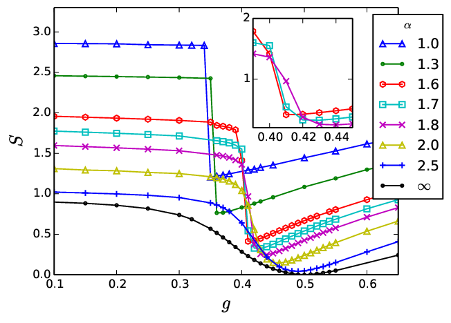
Fig.3 shows in particular dependence of entanglement on for several values of . At , there are two turning points for the curve: The first one is related to the dimerization transition point at (where a gap opens and entanglement drops), but it is difficult to locate accurately from entanglement; The other one is the minimum of entanglement just at the Majudar-Ghosh point . The two points are smoothly connected and approaches as reduces until the point (see inset of Fig.3), indicating shrinking of the VBS(comm.) phase and finally terminating at that point. That multi-critical point is in agreement with the ED result obtained by extrapolation [10]. The trajectory of as changes appears as a valley in the entanglement plane of Fig.2, where it should also have minimum correlation length, and thus can be thought of as a disorder-line[36], separating phases with commensurate and incommensurate correlation on either side. After the multi-critical point, entanglement becomes discontinuous displaying a sudden deep drop, which clearly marks the first order phase transition from the AFM phase to the decoupled phase [10].

The rather high amount of entanglement in the AFM phase poses considerable difficulties to the MPS method, since the computational effort for it scales exponentially with entanglement [17]. Here we would like to elaborate on these difficulties. Fig.4(a) shows dependence of both average variance and entanglement on at . This serves as a benchmark of the accuracy viable. One can see that variance increases radically with decreasing . These restrict us to for the variance smaller than 1e-4 for the maximal length and largest used. And we find much more sweeps (around 10 times) needed for convergence for small . Further more, there is metastable state issue to the left of the first order transition point. As shown in Fig.4(b), it is prone to get stuck on an excitation level which should have less entanglement than the ground state, if one uses random state or iDMRG for an initial state. This leads to a wrong position of the peak of energy (the transition point) compared with ED[10]. For a given , larger can shrink the region being stuck, but soon become unpractical. A two-site algorithm with density matrix correction won’t solve it either. It turns out a nice solution is to provide a better initial state, e.g., use the state of a smaller as the input of larger close to the right of the boundary (see [37] for alternative ways such as adding a pinning term for fixing this). In this way, the peaks for each lengths are unambiguously determined and the extrapolated value of the transition point is (see inset of Fig.4(b)). As for the infinite algorithm, the metastable issue is more severe. It is stuck in a wider range, which, we however haven’t found a way to avoid. For close to 0 the energy still deviates with VMPS. This is not because of getting stuck but is a convergence problem due to too fast growing of entanglement and at the same time relatively slow convergence of energy. As shown in Fig.4(c), entanglement suddenly drops after around 30 iteration steps (120 chain length) if is kept not increased and eventually converged to a wrong fixed point. One could stop iteration before the drop (this is where the data points of energy we adopted), but energy and other quantity are far from convergence. In all we find good convergence of VMPS for the parameter range studied, while iDMRG has either metastable state or convergence problems in the AFM phase.
III.2 scaling of entanglement under LRI


As shown above, the highest amount of entanglement is found when frustration is zero and is small. At , according to previous ED [10] and quantum Monte Carlo [9] studies, the system undergoes a continuous phase transition from the QLRO to AFM phase at . Recall that for a conformal invariant system with open boundary condition, the entanglement scales logarithmically with subsystem length [17, *calabrese2004entanglement, *holzhey1994geometric]
| (7) |
where in the prefactor is identified with the central charge of the relevant field theory. The QLRO phase belongs to this category and has . We expect changing of behaviour of around , and wonder to what extent the entanglement in the AFM phase with strong LRI violates the area law.
To this end, we focus primarily on the line of and use both VMPS and iDMRG to simulate various sized systems. The former, being free of environment error [38] and better controlled, is used for , while the later having reduced computation cost, is used for and validated by the consistency with small chains. We first present for the largest size for each in Fig.5(a). One can see remarkably that, for all values scales approximately logarithmically with (for not too close to the chain center), and that increases clearly faster for smaller . To quantify and compare them, it is tempting to use Eq.7 to fit each curve and extract a value of . We may call generally an “effective central charge”, as the AFM phase is not conformal invariant [9]. As shown in the inset of Fig.5(a), is near to 1.0 for , after that, it increases quickly with and reaches a large value. This behaviour is in overall agreement with the transition point .
The above extracted values of in the AFM phase are, however, not quite validated. For one thing, closely examining the fitting, one finds small deviations from perfect logarithm: seemingly increases slightly faster for larger . For another, and more significantly, actually has a salient dependence on the total system size, as a result the values are only specific to . To manifest this finite size effect on , we compare three points (1.0, 0.0), (1.0, 0.7) and (3.0, 0.0) which are respectively representatives of the AFM, decoupled, and QLRO phases. For each point we plot for various system sizes, as shown in Fig5(b). Since they all have (approximately) logarithm divergence, the values of are extracted for each , and shown in the inset of the graph. One can find that a clear dependence of and on is unique to the AFM phase. (In the decoupled phase, are close to 2.0, which is expected. Because, as will be shown later, it is a system of two approximate Heisenberg chain, whose central charge is just the sum of each one’s.) The dependence of on implies that the maximal size should be not enough. We will try to give an extrapolated result for it later, but below we first try to interpret the results obtained.
So far in the above we observed that for all values, have approximately logarithm dependence, while the slope i) apparently increases for smaller , ii) slightly increases for larger and iii) increases for larger . We give a naive explanation for these from a valence-bond description of the singlet ground state of antiferromagnet. A valence-bond is a singlet pair , where and are on opposite sublattices of of a bipartite lattice. It is known that, a SU(2) singlet ground state can always be represented in a valence-bond basis which is all possible covering of singlet pairs on the chain for even . Each singlet pair is maximally entangled, and the value is . Thus bipartite entanglement can be measured as the number of bonds cut by the bipartition times [39, *chhajlany2007topological]. This give a appealing geometrical interpretation of the ground state entanglement. For the Heisenberg model, favors forming of singlet between spin and , but many body effects eventually leads to forming of complex distribution of configurations of valence-bond [40] — including pairs apart in arbitrarily long distances. Note it is the long distance entangled pairs that lead to divergence of entanglement with increasing . Notably, for the unfrustrated regime of the Hamiltonian 1, long-range terms (we may call them bonds of the Hamiltonian) favor directly long distance singlet pairs. It is then reasonable to assume that the number of valence-bond in the ground state across and is in a way positively correlated with the sum of the strength of all bonds of the Hamiltonian across them, i.e. with the quantity
| (8) |
(Note that we can safely ignore the normalization in the Hamiltonian when .) Based on this, we may understand the properties just stated. For i), increases with smaller , so entanglement increases faster as well. (But this does not explain why they are close to logarithm for all the ); For ii) and iii), sums over (approximately for large and small ) bonds, while in contrast, for the QLRO phase which is essentially short-ranged, there is always only one bond connects the two regions irrespective of the position of the cut or the system size. This helps to understand why in the AFM phase the approximate logarithm function increases even faster when or expands, while it does not in the QLRO phase.


To get a glance of in he thermodynamical limit, we try to extrapolate the values in for each fixed and . Hereafter we make the dependence of on , and explicit, leaving fixed implicit. In Fig.6(a) we fix and show for different the dependence of ) on . In Fig.6(b), we fix and show for different the dependence of on . They show that the extrapolation is plausible. For different and there is always a relation
| (9) |
but with a non-travail coefficient depending on and . Two profiles of for fixed or are shown in the insets of Fig.6(a) and (b). The finite size effect is more salient for smaller or larger . This is in agreement with the above argument from the valence-bond description.
Then extrapolated for more and combinations are shown in Fig.6(c). Note that it should be understood as a result for semi-infinite chain . One can see that each curve is still close to a logarithm function, with the slop slightly increases with larger . The maximal evaluated is rather restricted, it is not very clear whether keeps increasing slowly or approaches a constant for even larger . For the former, the function form can be e.g. , while for the later, it can be e.g. . We have verified that both can give a good fit for the curves (not shown), other than a simple logarithm function. But in view of the correction in Eq.9, and that in Fig.5(b) curves for different are all close to logarithm functions, we are prone to the later.
III.3 phase boundary at moderate frustration

We next turn to the right part of the phase diagram. Focusing on one line , we measure the spin correlation
| (10) |
and see how it changes as reduces. Here the spin chain is considered to be divided into odd and even sublattices, as is usually did for the model. Fig.7 shows correlation between spins within a same sublattice (even ). One can see that for large values decreases exponentially with jumps in the curve. The jumps signify the incommensurate behaviour: Following the treatment of White and Affleck [7] of the model, we multiplying e.g. at and by , then the sinusoidal modulation is clearly seen in the inset of the graph, where the correlation length is chosen such that the beats of the amplitude are as flat as possible. By evaluating for up to 1000, we only find jumps for . For , displays algebraical decay (for reference with at ). This indicates a possible critical value of a continuous phase transition at roughly 1.2.

In previous studies with short chains, Sandvik [10] estimates that the transition should be from the VBS phase to a coexisting VBS+QLRO() phase, while Kumar and Soos [11] predict that the transition is from VBS phase to a decoupled phase. We agree with Kumar and Soos that for small there should be no VBS order and is essentially decoupled, but from an independent and more direct way: In fact the correlation shown above already implies no VBS order for , because the presence of incommensurate behaviour is related to a finite dimerization [7]. We also show directly the dimerization order parameter [6, 7] for several tuples in Fig.8(a). One can see that, for , are clearly nonzero; While for , are very small and appear to vanish in the limit . In addition, the inter-chain correlation is very small for , as shown in Fig.8(b). (Here it suffices to consider for , since further decays for larger odd .)
The transition points for other can be determined likewise and we find that increases with , and it should be that as . This gives a approximate phase boundary between VBS(incomm.) and the decoupled phase in Fig.1. Note crucially that the starting point of the phase boundary is distinct from both Kumar and Soos’s or Sandvik’s result, in which, it starts at a unique multi-critical at around (1.7, 0.41). The significance of this is that there indeed can be direct transition from AFM long-range order to VBS order [10].
The phase transition can be understood as follows: At moderate or large , as reduces, the couplings for (including ) all become very small due to a large normalization factor, and eventually the next-nearest neighbour term dominates. The later induce a background of antiferromagnetic order on either sublattices, this amounting to a period 4 structure in the entire lattice. It is not difficult to see that, the rest enormous but small couplings now have conflicting signs against this background period, and their effects should be largely smeared out. So for mall enough it is decoupled into nearest-neighboured Heisenberg model with coupling and with long-range terms as perturbations. Note that for the model (), White and Affleck [7] used field theory to predict that there is exponential small gap and dimerization for arbitrary large , except for where it decouples exactly into two Heisenberg chain, and supported it by DMRG. While our arguments above essentially states that, at small , the spin chain can be decoupled for modest . Nevertheless, the evaluation of is still not very long and the decay of with is somewhat slow, so we are still not completely sure whether there are incommensurate modulation with very long period or dimerization (and also spin gap) should be exponentially small but nonzero even as approaches 0, which is very difficult to confirm numerically. A field theory study for small may be desirable as well as that for the model at large .
IV conclusion
In summary, we studied the frustrated spin chain with long-range interactions using the matrix product state approaches. We found that it is most entangled in the rotation invariant AFM long-range ordered phase, where the entanglement scales approximately in logarithmic form. But we miss a complete understanding for the logarithmic scaling. The maximal systems size studied is not large and is still not close to 0. It is worthwhile to check the persistence of the logarithmic form in the asymptotic scaling of entanglement for large subsystem size and smaller in future works. We also studied correlation and dimerization for moderate frustration and determined an approximate boundary for the transition from the dimerized and incommensurate phase of the model to a decoupled phase.
Our work implies that in an antiferromagnetic spin chain with LRI, frustration terms usually hamper long-range entanglement. Consider a series of power law decayed models , with the signs while indeterminate. At small , their entanglement should be bounded by the unique nonfrustrated one i.e. , where perfect AFM long-range order is formed.
The scaling of entanglement shown in this work and previous works [21, 22] indicates that, although LRI can usually increase entanglement, but it not necessarily leads to large entanglement and severe violation of area law. The preservation or (severe) violation of area law may be a joint effects of interaction range, symmetry constrains (e.g. translation invariance), ground state degeneracy, and etc, which remains to be clarified.
acknowledgement
ZHL thanks A.W. Sandvik and M.Q. Weng for valuable discussions. We acknowledge an anonymous referee whose comment induced us to do a systematic analysis on the finite size effect on entanglement scaling. This work is supported by National Natural Science Foundation of China under Grant No. 11375168. The simulation is mainly conducted on the Supercomputing system in the Supercomputing Center of USTC.
References
References
- [1] I. Affleck, D. Gepner, H. J. Schulz, and T. Ziman, J. Phys. A: Math. Gen. 22, 511 (1989).
- [2] T. Giamarchi and H. J. Schulz, Phys. Rev. B 39, 4620 (1989).
- [3] K. Okamoto and K. Nomura, Phys. Lett. A 169, 433 (1992).
- [4] S. Eggert, Phys. Rev. B 54, R9612 (1996).
- [5] C. K. Majumdar and D. K. Ghosh, J. Math. Phys. 10, 1388 (1969).
- [6] R. Bursill, G. A. Gehring, D. J. J. Farnell, J. B. Parkinson, T. Xiang, and C. Zeng, J. Phys.: Condens. Matter 7, 8605 (1995).
- [7] S. R. White and I. Affleck, Phys. Rev. B 54, 9862 (1996).
- [8] E. Yusuf, A. Joshi, and K. Yang, Phys. Rev. B 69, 144412 (2004).
- [9] N. Laflorencie, I. Affleck, and M. Berciu, J. Stat. Mech. Theor. Exp. 2005, P12001 (2005).
- [10] A. W. Sandvik, Phys. Rev. Lett. 104, 137204 (2010).
- [11] M. Kumar and Z. G. Soos, Phys. Rev. B 88, 134412 (2013).
- [12] J.-C. Tung and G.-Y. Guo, Phys. Rev. B 83, 144403 (2011).
- [13] L. Amico, R. Fazio, A. Osterloh, and V. Vedral, Rev. Mod. Phys. 80, 517 (2008).
- [14] M. Srednicki, Phys. Rev. Lett. 71, 666 (1993).
- [15] J. Eisert, M. Cramer, and M. B. Plenio, Rev. Mod. Phys. 82, 277 (2010).
- [16] M. B. Hastings, J. Stat. Mech. Theor. Exp. 2007, P08024 (2007).
- [17] G. Vidal, J. I. Latorre, E. Rico, and A. Kitaev, Phys. Rev. Lett. 90, 227902 (2003).
- [18] P. Calabrese and J. Cardy, J. Stat. Mech. Theor. Exp. 2004, P06002 (2004).
- [19] C. Holzhey, F. Larsen, and F. Wilczek, Nucl. Phys. B 424, 443 (1994).
- [20] J. I. Cirac and F. Verstraete, J. Phys. A: Math. Theor. 42, 504004 (2009).
- [21] J. I. Latorre, R. Orús, E. Rico, and J. Vidal, Phys. Rev. A 71, 064101 (2005).
- [22] T. Koffel, M. Lewenstein, and L. Tagliacozzo, Phys. Rev. Lett. 109, 267203 (2012).
- [23] S. R. White, Phys. Rev. Lett. 69, 2863 (1992).
- [24] S. R. White, Phys. Rev. B 48, 10345 (1993).
- [25] G. M. Crosswhite, A. C. Doherty, and G. Vidal, Phys. Rev. B 78, 035116 (2008).
- [26] In Eq.1, diverges for infinite when , which seems impossible to represent numerically. But in the long range MPO method, the power function coupling is actually approximated with a by the sum of several exponential functions and decays exponentially in large distance. So [and also ] do converge in practice.
- [27] F. Fröwis, V. Nebendahl, and W. Dür, Phys. Rev. A 81, 062337 (2010).
- [28] U. Schollwöck, Ann. Phys. 326, 96 (2011).
- [29] J. Dukelsky, M. A. Martín-Delgado, T. Nishino, and G. Sierra, Europhys. Lett. 43, 457 (1998).
- [30] F. Verstraete, D. Porras, and J. I. Cirac, Phys. Rev. Lett. 93, 227205 (2004).
- [31] I. P. McCulloch, J. Stat. Mech. Theor. Exp. 2007, P10014 (2007).
- [32] S. R. White, Phys. Rev. B 72, 180403 (2005).
- [33] I. P. McCulloch, arXiv:0804.2509 [cond-mat] (2008).
- [34] S. Rommer and S. Östlund, Phys. Rev. B 55, 2164 (1997).
- [35] The starting point of this phase boundary chose by Sandvik is , while we use . This is a matter of angle viewing the commensurate/incommensurate transition either from momentum space or real space. This is discussed in detail in \rev@citealpnumbursill1995numerical.
- [36] R. Chitra, S. Pati, H. R. Krishnamurthy, D. Sen, and S. Ramasesha, Phys. Rev. B 52, 6581 (1995).
- [37] E. Stoudenmire and S. R. White, Annu. Rev. Condens. Matter Phys. 3, 111 (2012).
- [38] U. Schollwöck, Rev. Mod. Phys. 77, 259 (2005).
- [39] F. Alet, I. P. McCulloch, S. Capponi, and M. Mambrini, Phys. Rev. B 82, 094452 (2010).
- [40] R. W. Chhajlany, P. Tomczak, and A. Wójcik, Phys. Rev. Lett. 99, 167204 (2007).