GMC Collisions as Triggers of Star Formation. I.
Parameter space exploration with 2D simulations
Abstract
We utilize magnetohydrodynamic (MHD) simulations to develop a numerical model for GMC-GMC collisions between nearly magnetically critical clouds. The goal is to determine if, and under what circumstances, cloud collisions can cause pre-existing magnetically subcritical clumps to become supercritical and undergo gravitational collapse. We first develop and implement new photodissociation region (PDR) based heating and cooling functions that span the atomic to molecular transition, creating a multiphase ISM and allowing modeling of non-equilibrium temperature structures. Then in 2D and with ideal MHD, we explore a wide parameter space of magnetic field strength, magnetic field geometry, collision velocity, and impact parameter, and compare isolated versus colliding clouds. We find factors of increase in mean clump density from typical collisions, with strong dependence on collision velocity and magnetic field strength, but ultimately limited by flux-freezing in 2D geometries. For geometries enabling flow along magnetic field lines, greater degrees of collapse are seen. We discuss observational diagnostics of cloud collisions, focussing on 13CO(=2-1), 13CO(=3-2), and 12CO(=8-7) integrated intensity maps and spectra, which we synthesize from our simulation outputs. We find the ratio of =8-7 to lower- emission is a powerful diagnostic probe of GMC collisions.
Subject headings
ISM: molecular clouds — ISM: magnetic fields — methods: numericalI. Introduction
Understanding star formation is a key astrophysical problem, with many fundamental questions still unresolved. In particular, what mechanisms drive or inhibit the star formation process? Studying the evolution of giant molecular clouds (GMCs) within the diffuse interstellar medium and the formation of prestellar clumps and cores within GMCs is complicated because of the large range of densities ( to ), length scales (kpc to 0.1 pc), and timescales ( yr for galactic orbits to yr for core dynamical timescales) involved, as well as the nonlinear effects of self-gravity, thermal, magnetic, and turbulent pressures, large-scale motions such as galactic shear or collisional converging flows, radiation, chemistry, and feedback. Additionally, the initial conditions are uncertain and boundary conditions are poorly constrained. The final conditions, gleaned through observations, suggest that star formation is highly clustered and localized, with relatively high local efficiency within clusters (Lada & Lada 2003; Gutermuth et al. 2009, e.g.,). However, overall star formation is slow and inefficient, with only a few percent of total gas forming stars over local dynamical timescales (Zuckerman & Evans 1974; Krumholz & Tan 2007; Da Rio et al. 2014, e.g.,).
With regard to the importance of magnetic fields (Crutcher 2012; Li et al. 2014, see, e.g.,), there have been two main views. Strong-field models propose relatively long GMC lifetimes in which magnetic fields play important roles in controlling formation and evolution of the clouds. In these models, non-star-forming clouds are initially subcritical, i.e., their magnetic fields are strong enough to prevent gravitational collapse. Weak-field models have GMCs as intermittent phenomena with short lifetimes ( yr) and turbulent flows controlling the formation of clouds, clumps and cores. These models posit magnetically supercritical masses, i.e., the magnetic pressure alone is too weak to support against gravity.
Zeeman measurements show that mass-to-magnetic flux ratios () are approximately critical to slightly supercritical in molecular clouds (Crutcher 1999; Troland & Crutcher 2008; Crutcher 2012; Li et al. 2014). If GMCs are partially stabilized by magnetic fields, then this may increase their lifetimes to Myr timescales, which are then comparable to GMC-GMC collision times, especially for clouds inside the solar circle (Gammie et al. 1991; Tan 2000; Tasker & Tan 2009; Dobbs et al. 2015). Indirect observational evidence for frequent GMC collisions comes from the near random orientations of projected angular momentum vectors of GMCs (Rosolowsky et al. 2003; Koda et al. 2006; Imara & Blitz 2011; Imara et al. 2011).
Frequent GMC collisions could be an important mechanism for injecting turbulent energy into GMCs (Tan 2000; Tan et al. 2013), with the energy being extracted from galactic orbital motion. Other mechanisms for injecting turbulence involve star formation feedback (Matzner 2007; Goldbaum et al. 2011). Without such replenishment, turbulence is expected to decay within about a crossing time (Mac Low et al. 1998; Ostriker et al. 1999).
By producing dense gas, compressed in shocks, GMC-GMC collisions may be an important trigger of star cluster formation (Scoville et al. 1986). If the majority of star formation is initiated by this process, then a model of shear-mediated cloud collisions can naturally explain the observed dynamical Kennicutt-Schmidt relation (Kennicutt 1998) in which a roughly constant fraction of gas, is converted into stars every local orbital time (Tan 2000; Tan 2010; Suwannajak et al. 2014). Note that this mechanism of creating star-forming molecular clumps from localized compressed regions of pre-existing GMCs, is different from that proposed for creating molecular clouds from shocks in converging flows of atomic gas (Heitsch et al. 2006; van Loo et al. 2007; Heitsch et al. 2009; van Loo et al. 2010, e.g.,).
Cloud-cloud collisions have been investigated by a number of previous studies. Habe & Ohta (1992) performed 2D axisymmetric SPH simulations of head-on collisions of non-identical clouds. These collisions produced a bow shock which disrupted the larger cloud while compressing the smaller cloud. This compression could lead to gravitational instability for the smaller cloud even if its initial mass was below the Jeans mass.
Klein & Woods (1998) presented 2D AMR hydrodynamics simulations of homogeneous cloud collisions. The collisions resulted in bending mode instabilities creating large aspect ratio filaments. With surface perturbations, the merged cloud system became highly asymmetrical and highly inhomogeneous with islands of high density surrounded by low density regions.
Anathpindika (2009) performed a series of 3D SPH simulations which investigated the gravitational stability of post-shock compressed slabs resulting from molecular cloud collisions. Additionally, sheared collisions result in non linear thin shell instabilities and Kelvin-Helmholtz instabilities.
More recently, Takahira et al. (2014) performed 3D hydrodynamic simulations with AMR showing core formation occurring from a GMC collision interface. They found that faster collision velocities formed a greater number of cores, but core growth was predominantly via accretion in the shock front, with slower shocks being favored for making larger cores.
In terms of MHD collision studies, Körtgen & Banerjee (2015) investigated molecular cloud formation and the transition from magnetically sub- to supercritical HI clouds via converging magnetized flows. Even with magnetic diffusion effects, they found that cylindrical flows created no magnetically supercritical regions and star formation is strongly suppressed for even relatively low initial magnetic field strengths.
This paper, the first of a series, explores the process of magnetized cloud-cloud collisions and its effect on individual GMC and clump scales. Here we restrict analysis to a parameter space exploration with 2D simulations of simplified cloud geometries, including an embedded clump: formally colliding infinite cylinders, which can approximate collisions of spheroidal clouds.
§II explains the fiducial set-up and various simulation and analytic methods employed. §III describes new heating and cooling functions that we have developed for this project. §IV describes the set up and subsequent results of exploring the following parameters: magnetic field strength, magnetic field orientation, collision velocity, and impact parameter. §V discusses predictions of observational diagnostics of shocks. Discussion and conclusions follow in §VI.
II. Numerical Model
II.1. Initial Conditions
For our default initial conditions we use typical observed values of Galactic GMC and ISM properties. GMCs are conventionally defined as having masses . They have mean mass surface densities (McKee & Ostriker 2007; Tan et al. 2013, e.g.,). Typical mean volume densities are , although clumps and cores within the clouds have densities that can be orders of magnitude larger.
GMCs have internal velocity dispersions that are similar to virial velocities, typically several km/s, which is much larger than the km/s sound speeds of K gas. Supersonic turbulence and self-gravity are thought to be two important processes that help give rise to the hierarchical density structures seen in GMCs. However, these structures may also be regulated by magnetic fields.
The magnetic field of the local diffuse ISM background is (Beck 2001). If a random, uniform distribution of field strengths is assumed up to a maximum value, , Zeeman measurements reveal that this maximum magnetic field value measured within molecular clouds, clumps and cores with scales as , where (Crutcher et al. 2010). At lower densities, , independent of density. We will henceforth refer to this as the “Crutcher relation”. Thus, for , .
Observed random velocities of Galactic GMCs are approximately 5-7 (Liszt et al. 1984; Stark 1984, e.g.,). However, interaction velocities between colliding GMCs are likely to be set by the shear velocity at 1 to 2 tidal radii of the clouds (Gammie et al. 1991; Tan 2000), which can be several times larger.
Given the 2D nature of the simulations of this paper, the modeled structures can be considered as filaments extending perpendicular to the simulation domain. We follow “clouds”, i.e., “GMCs,” with a uniform density of . Although the clouds are, in principle, cylinders of infinite extent, we assume that the clouds have a finite mass, i.e., . A mass surface density of integrated along the cloud axis, then, gives a typical cloud radius pc. We set the radius of the first cloud, i.e., Cloud 1, to and of the second one, i.e., Cloud 2, to .
GMCs are structured, containing dense clumps. When a collision occurs, the effect of this collision on pre-existing clumps may be the most important for triggering star formation. We therefore introduce an idealized embedded, overdense clump into Cloud 1. The clump has a uniform density of , i.e., overdense compared to the GMC, and a radius of 5.6 pc. We position the clump off center at (see Fig. 1). The properties of our clouds and clump are listed in Table 1.
| 11 1 Masses are for an equivalent spherical cloud. | 22 2 Critical -field strengths are listed for the GMCs and the clump, along with the fiducial ambient field strength. | |||
|---|---|---|---|---|
| Ambient | - | 10 | - | 10 |
| GMC 133 3 GMC 1 includes a clump, but properties listed here are for non-clump material within the cloud | 1.78 | 100 | 23.8 | 42.0 |
| GMC 2 | 0.56 | 100 | 11.9 | 13.9 |
| Clump | 0.10 | 1000 | 5.64 | 66.0 |

For typical molecular cloud temperatures, K, such GMCs and clumps are not thermally supported against gravitational collapse. For example, if the clouds are considered as long filaments in the direction perpendicular to the simulation plane, then the mass per unit length for GMC 1, , far exceeds the critical line mass for a cylindrical cloud, given by , which is for a cold K cloud (Ostriker 1964).
The inclusion of magnetic fields helps to stabilize the clouds. We vary the direction, i.e., parallel, perpendicular and oblique to the cylindrical axis of the cloud, and the magnitude of the field. The field strengths are detailed in the results section, but are of the order of , given observed field strengths (Crutcher 2012).
Internal cloud turbulence is another mechanism that may help support GMCs. To separate out the effects of magnetic fields from turbulence, in this paper we do not initialize the clouds with any turbulence, deferring this to Paper II, which also extends the dimensionality to 3D. However, turbulent motions are generated by the GMC-GMC collision, which may then provide additional support to the clouds.
The ambient medium in which the clouds are embedded, representative of the atomic cold neutral medium, is set to have , with a magnetic field of . The default relative collision velocity of the clouds is set to be , with variations from 5 to 40 . The default impact parameter, , of the collision is set to zero, i.e., an on-axis collision, but some cases with are also explored. The surrounding medium, which we consider to be a co-moving atomic envelope around the GMC, is also colliding. Thus in terms of the simulation domain, half the box is moving with and the other half has . However, at faster velocities we sometimes notice modest effects of numerical viscosity on clump properties and so also run simulations in the velocity frame of Cloud 1.
A summary of key parameters in all runs performed in this paper is listed in Table 2. Velocities denoted with a “*” indicate models run in the frame of Cloud 1.
| Run | ||||||||||
|---|---|---|---|---|---|---|---|---|---|---|
| (cm-3) | (cm-3) | (cm-3) | (cm-3) | () | () | () | () | (km/s) | () | |
| 0. Out-of-plane Fields | ||||||||||
| 0. Isolated Cloud | ||||||||||
| 0.A.0 | 10 | 100 | - | - | (0,0,10) | (0,0,27.9) | - | - | - | - |
| 0.A.1 | 10 | 100 | - | - | (0,0,0) | (0,0,0) | - | - | - | - |
| 0.A.2 | 10 | 100 | - | - | (0,0,10) | (0,0,10) | - | - | - | - |
| 0.A.3 | 10 | 100 | - | - | (0,0,10) | (0,0,20) | - | - | - | - |
| 0.A.4 | 10 | 100 | - | - | (0,0,10) | (0,0,40) | - | - | - | - |
| 1. Out-of-plane Fields | ||||||||||
| 1.B. Isolated Cloud with Clump | ||||||||||
| 1.B.0 | 10 | 100 | 1000 | - | (0,0,10) | (0,0,40) | (0,0,65) | - | - | - |
| 1.B.1.1 | 10 | 100 | 1000 | - | (0,0,10) | (0,0,10) | (0,0,65) | - | - | - |
| 1.B.1.2 | 10 | 100 | 1000 | - | (0,0,10) | (0,0,20) | (0,0,65) | - | - | - |
| 1.B.1.3 | 10 | 100 | 1000 | - | (0,0,10) | (0,0,65) | (0,0,65) | - | - | - |
| 1.B.2.1 | 10 | 100 | 1000 | - | (0,0,10) | (0,0,40) | (0,0,40) | - | - | - |
| 1.B.2.2 | 10 | 100 | 1000 | - | (0,0,10) | (0,0,40) | (0,0,55) | - | - | - |
| 1.B.2.3 | 10 | 100 | 1000 | - | (0,0,10) | (0,0,40) | (0,0,75) | - | - | - |
| 1.C. Cloud Collision | ||||||||||
| 1.C.0 | 10 | 100 | 1000 | 100 | (0,0,10) | (0,0,40) | (0,0,65) | (0,0,13.2) | 10 | 0 |
| 1.C.1.1 | 10 | 100 | 1000 | 100 | (0,0,10) | (0,0,40) | (0,0,65) | (0,0,13.2) | 5 | 0 |
| 1.C.1.2 | 10 | 100 | 1000 | 100 | (0,0,10) | (0,0,40) | (0,0,65) | (0,0,13.2) | 20* | 0 |
| 1.C.1.3 | 10 | 100 | 1000 | 100 | (0,0,10) | (0,0,40) | (0,0,65) | (0,0,13.2) | 40* | 0 |
| 1.C.2.2 | 10 | 100 | 1000 | 100 | (0,0,10) | (0,0,40) | (0,0,65) | (0,0,13.2) | 10 | 0.5 |
| 1.C.2.4 | 10 | 100 | 1000 | 100 | (0,0,10) | (0,0,40) | (0,0,65) | (0,0,13.2) | 10 | 1 |
| 1.C.2.5 | 10 | 100 | 1000 | 100 | (0,0,10) | (0,0,40) | (0,0,65) | (0,0,13.2) | 10 | 1.5 |
| 2. In-plane Fields and | ||||||||||
| 2.B. Isolated Cloud with Clump | ||||||||||
| 2.B.1.0 | 10 | 100 | 1000 | - | (40,0,0) | (40,0,0) | (40,0,0) | - | - | - |
| 2.B.1.1 | 10 | 100 | 1000 | - | (10,0,0) | (10,0,0) | (10,0,0) | - | - | - |
| 2.B.1.2 | 10 | 100 | 1000 | - | (65,0,0) | (65,0,0) | (65,0,0) | - | - | - |
| 2.B.2.0 | 10 | 100 | 1000 | - | (0,40,0) | (0,40,0) | (0,40,0) | - | - | - |
| 2.B.2.1 | 10 | 100 | 1000 | - | (0,10,0) | (0,10,0) | (0,10,0) | - | - | - |
| 2.B.2.2 | 10 | 100 | 1000 | - | (0,65,0) | (0,65,0) | (0,65,0) | - | - | - |
| 2.C. Cloud Collision | ||||||||||
| 2.C.1.0 | 10 | 100 | 1000 | 100 | (40,0,0) | (40,0,0) | (40,0,0) | (40,0,0) | 10 | 0 |
| 2.C.1.1 | 10 | 100 | 1000 | 100 | (10,0,0) | (10,0,0) | (10,0,0) | (10,0,0) | 10 | 0 |
| 2.C.1.2 | 10 | 100 | 1000 | 100 | (65,0,0) | (65,0,0) | (65,0,0) | (65,0,0) | 10 | 0 |
| 2.C.2.0 | 10 | 100 | 1000 | 100 | (0,40,0) | (0,40,0) | (0,40,0) | (0,40,0) | 10 | 0 |
| 2.C.2.1 | 10 | 100 | 1000 | 100 | (0,10,0) | (0,10,0) | (0,10,0) | (0,10,0) | 10 | 0 |
| 2.C.2.2 | 10 | 100 | 1000 | 100 | (0,35,0) | (0,65,0) | (0,65,0) | (0,65,0) | 10 | 0 |
| 3. Mixed Fields | ||||||||||
| 3.B. Isolated Cloud with Clump | ||||||||||
| 3.B.1 | 10 | 100 | 1000 | - | (10,0,0) | (10,0,38.7) | (10,0,64.2) | - | - | - |
| 3.B.2 | 10 | 100 | 1000 | - | (0,10,0) | (0,10,38.7) | (0,10,64.2) | - | - | - |
| 3.C. Cloud Collision | ||||||||||
| 3.C.1.0 | 10 | 100 | 1000 | 100 | (10,0,0) | (10,0,38.7) | (10,0,64.2) | (10,0,12.9) | 10 | 0 |
| 3.C.1.1 | 10 | 100 | 1000 | 100 | (10,0,0) | (10,0,38.7) | (10,0,64.2) | (10,0,12.9) | 5 | 0 |
| 3.C.1.2 | 10 | 100 | 1000 | 100 | (10,0,0) | (10,0,38.7) | (10,0,64.2) | (10,0,12.9) | 20* | 0 |
| 3.C.1.3 | 10 | 100 | 1000 | 100 | (10,0,0) | (10,0,38.7) | (10,0,64.2) | (10,0,12.9) | 40* | 0 |
| 3.C.2.0 | 10 | 100 | 1000 | 100 | (0,10,0) | (0,10,38.7) | (0,10,64.2) | (0,10,12.9) | 10 | 0 |
| 3.C.2.1 | 10 | 100 | 1000 | 100 | (0,10,0) | (0,10,38.7) | (0,10,64.2) | (0,10,12.9) | 5 | 0 |
| 3.C.2.2 | 10 | 100 | 1000 | 100 | (0,10,0) | (0,10,38.7) | (0,10,64.2) | (0,10,12.9) | 20* | 0 |
| 3.C.2.3 | 10 | 100 | 1000 | 100 | (0,10,0) | (0,10,38.7) | (0,10,64.2) | (0,10,12.9) | 40* | 0 |
| 3.D. Cloud Collision with Impact Parameter | ||||||||||
| 3.D.0 | 10 | 100 | 1000 | 100 | (10,0,0) | (10,0,38.7) | (10,0,64.2) | (10,0,12.9) | 10 | 0.5 |
II.2. Numerical Code
The numerical code is a modified version of the Adaptive Mesh Refinement (AMR) code Enzo 2.0 (Bryan & Norman 1997; Bryan 1999; O’Shea et al. 2004). To solve the magnetohydrodynamical equations, we use a 2nd-order Runge-Kutta temporal update of the conserved variables with the Local Lax-Friedrichs (LLF) Riemann solver and a piecewise linear reconstruction method. To ensure the solenoidal constraint on the magnetic field, the divergence cleaning algorithm of Dedner et al. (2002) is adopted (Wang & Abel 2008).
We implemented heating and cooling functions in the code that describe both atomic and molecular heating and cooling processes (see §III for details). These functions take into account a density versus column density extinction relation similar to that of Van Loo et al. (2013, henceforth, VLBT2013). As the temperature of the gas needs to be calculated accurately, we use a “dual energy formalism” by solving the internal energy equation as well as the total energy equation. The temperature is then determined from the internal pressure when magnetic and kinetic energy together exceed 0.999 the total energy, and from the total energy otherwise.
To track the evolution of properties of the clump, we use a scalar value to differentiate between gas outside and inside the clump. We set the scalar to 1 inside the clump and 0 outside. We added a conservation equation in Enzo 2.0 to advect the scalar, i.e.,
| (1) |
with the cell density and the velocity.
We model a numerical domain of 256pc2 which is covered by a uniform grid of 10242, giving a grid cell size of 0.25 pc. For the fiducial model, two additional AMR grid levels are included, thus increasing the effective resolution to 40962 with a grid cell size of 0.0625 pc on the finest level. This resolution is sufficient to study the transition from subcritical to supercritical clouds and clumps.
We use several criteria to determine refinement: a cell is refined when there is a strong local gradient of variables (i.e., when the relative slope across variable at index exceeds 0.4), when it is part of a shock front (defined by a relative pressure jump of ), and when the local Jeans length is not covered by at least 4 cells (Truelove et al. 1997, needed to avoid artificial fragmentation).
III. Heating and Cooling Functions
We model the thermal properties of the ISM using a Photo-Dissociation Region (PDR)-based method that follows and expands upon VLBT2013 and is detailed in the following subsections.
III.1. Implementation of Thermal Processes
Implementation into the Enzo code involves calculating the net heating rate for a given cell:
| (2) |
where is the heating rate and is the cooling rate. The net cooling rate introduces a cooling timescale: . The internal energy of the gas is defined by .
We adopt a mean particle mass of (valid for molecular gas with 1 He per 10 H and ignoring contributions from other species). For simplicity, this value of is adopted through the simulation domain, i.e., even in the ambient, “atomic” medium.
The dynamics of the simulation (and the objects of main interest) are dominated by gas at densities of , which correspond to equilibrium temperatures of K (details described below). Thus, we adopt the value of for the entire simulation domain. While this does not account for the excitation of rotational and vibrational modes of that would occur in shocks, we consider that this is the most appropriate single-valued choice of for our simulation set-up, given our focus on the dynamics of the dense molecular gas.
The chosen values of and set sound speeds of . Since is often shorter than the hydrodynamical time, the temperature and internal energy are sub-cycled and updated, assuming constant density, until the hydrodynamical time step is reached. This is more computationally efficient as a method for preventing excessive heating or cooling, than evolving all variables on timesteps equal to the cooling or heating times.
III.2. Density-Extinction Relation
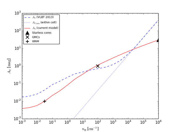
Simulating a region of a galactic disk, VLBT2013 found a monotonically increasing relation between density and average (six orthogonal ray) column extinction, which defined an effective visual extinction (Glover & Mac Low 2007). This relation was resolution-limited at high densities due to the effective visual extinction being dominated by absorption within a single 0.5 pc cell. For the simulations performed in this paper, we use a modified extinction curve normalized to estimated values of the Warm Neutral Medium (WNM): mag for (Wolfire et al. 2003), GMCs: mag for , and starless cores: mag for .
To fit these constraints as well as retain the physical relationships represented in the VLBT2013 curve, we ignore the effects of individual cell extinction at high densities and instead perform a logarithmic extrapolation from . This intermediate curve is fitted to the normalization points via a smooth scaling function, producing the final density-extinction relation (see Fig. 2).
III.3. Nonequilibrium PDR Heating and Cooling Rates
We next utilize both PyPDR 44 4 http://www.mpe.mpg.de/simonbr/research_pypdr/index.html (described below) and Cloudy (version 13.02, last described in Ferland et al. (2013)), photoionization simulation codes, to generate tables of non-equilibrium heating and cooling rates as functions of density, temperature and radiation field intensity. Our default value of FUV radiation field intensity is , following conditions developed for the kpc molecular ring region of the inner Milky Way (VLBT13). Then, given the vs. relation described in the last subsection, each value of density has a unique value of received FUV intensity, allowing a 2D () grid of heating and cooling rates to be sufficient. However, to calculate this 2D grid self-consistently does require calculation of arbitrary PDR models with input density, temperature and radiation field, in order to calculate species abundances correctly, especially of molecules like and CO that have abundances set by FUV photons whose propagation is affected by self-shielding.
To carry out these PDR models we primarily utilize PyPDR, which is a minimal Python-based PDR code that self-consistently calculates chemical, thermal, and molecular properties within a slab of gas irradiated with FUV photons.
PyPDR implements the same chemical network as in Röllig et al. (2007), which includes reactions for H2 formation, cosmic ray induced reactions, photodissociation (including self/mutual-shielding of H2, CO and C) and gas-phase reactions.
The following heating and cooling rates are implemented: H2 pumping and line cooling (Röllig et al. 2006), H2 formation (Sternberg & Dalgarno 1989), H2 dissociation (Jonkheid et al. 2004), gas-grain heating/cooling (Tielens 2005), photoelectric heating and recombination cooling (Bakes & Tielens 1994), Ly- cooling (Sternberg & Dalgarno 1989), optical Oxygen-6300 Å cooling (Sternberg & Dalgarno 1989), heating by C-ionization (Black & van Dishoeck 1987; Jonkheid et al. 2004), cosmic ray heating (Jonkheid et al. 2004), line cooling by OI, CII, CI (fine structure), CO and 13CO(rotational) calculated from the non-LTE excitation of OI, CII, CI, CO, and 13CO using an escape probability approach. Data from the LAMDA database (Schoeier et al. 2005) is used.
While the PyPDR chemical network includes only 30 atoms and molecules, it still performs well in benchmark tests, producing results similar to larger PDR codes (Röllig et al. 2007). However, as PyPDR was developed for temperatures only up to K, we do not use it for higher temperature conditions.
Cloudy, on the other hand, follows a much larger number of species than PyPDR and can treat K gas. Thus, we utilize it in this regime. However, for our purposes of defining non-equilibrium heating and cooling functions that utilize a two step process where high spectral resolution line self-shielding output is needed as a general input for the next PDR calculation, the public version of Cloudy does not automatically provide such output information. Thus we have adapted the PyPDR code of Bruderer for this purpose.
We set up the density-temperature parameter space for the arrays as follows. The density range is to , in steps of 0.1 dex (91 values) while the temperature spans from 2.7 K to K in steps of 0.046 dex (100 values). PyPDR was used to calculate the bulk of the rates, from T = 2.7 to K, while Cloudy was used for T = to K.
The procedure for both PDR codes generally follows that of VLBT2013, which used Cloudy version 8.02 and was based off of Smith et al. (2008). Any code-specific differences will be mentioned in the relevant sections.
First, the unextinguished local interstellar radiation field (ISRF) with is incident on an absorbing slab of gas with abundances, metallicities, and dust resembling that of the local ISM. We include the cosmic microwave background radiation as well as a background of cosmic rays with primary ionization rate of . The column density of the gas slab is determined by the previously described density-extinction relation and the linear relation between column density and visual extinction ( mag). For a given density, a PDR model is calculated through a slab with column corresponding to the particular density. In our case, the density of the slab also follows this given density, as the extinction should be dominated by the local density for GMC regions. Note, in VLBT13, the density of the slab was fixed at .
At the depth of the specified column (i.e., the final cell of the PDR model) the temperature of a parcel of gas is then varied, with heating and cooling rates calculated for the specific temperature. The calculations are repeated for the entire temperature range, yielding the temperature and density dependent heating and cooling functions.
In PyPDR, the code allows self-consistent calculation of general, nonequilibrium heating and cooling rates given species abundances set by equilbrium PDR conditions for given extinction, density and equilibrium temperature. The key PyPDR results for , , and abundances are shown in Fig. 3.

Arrays of heating and cooling rates were created using both PyPDR ( K to K) and Cloudy ( K to K), then smoothly joined along the temperature dimension using the function:
| (3) |
where is the final, smoothly combined rate, calculated from the gas temperature, the Cloudy rate, the PyPDR rate, and the Fermi-Dirac smoothing function:
| (4) |
This joined the functions at K, where good agreement still occurred between the models.
From the resulting final arrays of heating rates and cooling rates, a bilinear interpolation is performed to derive rates for any density and temperature combination. The final, combined 2D interpolation plots for cooling, heating, and net heating as functions of density and temperature are displayed in Fig. 4. These plots show the total cooling, heating, and net rate at all densities and temperatures.
Note, that from K up to K, we ignore heating and adopt the cooling rates derived by Sarazin & White (1987). Values beyond the array domain adopt the limiting values. Thus, for any cell in our Enzo simulation, the density and temperature are read in and cooling and heating rates are returned.


III.4. Heating and Cooling Components
A breakdown of specific heating and cooling components at the equilibrium temperature is shown in Fig. 5. Photoelectric heating of dust grains is the dominant heating source for low-density gas up until . Above this density, the higher dust extinction blocks external FUV photons and thus reduces photoelectric heating. The ubiquitous flux of cosmic rays then becomes the main heating component in high-density gas. formation also contributes as the cloud becomes fully molecular.
The main coolants in the low density, ionized/atomic region () are Ly- and Hydrogen recombination lines. As density increases, various atomic lines (OI, CII, CI) become dominant coolants. These species inelastically collide with H and He, exciting internal degrees of freedom and subsequently decaying through photon emission. Molecular lines (CO, 13CO) provide large contributions in cooling as density increases, temperature decreases, and the gas reaches high levels of molecular abundance. At the highest densities (), gas-grain cooling dominates as collisions between dust grains and gas molecules lead to emission of infrared photons from the decay of lattice vibrations.

III.5. Observational Diagnostics
In addition to providing a better understanding of the dominant physical processes occurring at different densities and temperatures, the heating/cooling component breakdown also enables the creation of observational diagnostics in the form of line emissivities. Here we focus on a preliminary investigation into high- CO to see if they are good diagnostics of shocks arising from cloud collisions. The PDR-derived cooling data include contributions from the first 40 rotational lines for both 12CO and 13CO. Similar to the method of creating the cooling and heating functions, tables of density and temperature dependent emissivities were compiled to allow calculation of observable quantities in the form of integrated intensity maps and spectra.
Via post-processing, integrated intensity maps can be derived from the volume emissivity functions coupled with simulation outputs. We assume a fixed 1 pc thickness of the simulation volume for calcuation of these maps. Given this simplistic, highly-idealized 2D geometry of cloud structures presented in this initial paper, for simplicity we do not calculate radiative transfer of the emissivities from each cell, but simply sum their contributions as if their emission reached us with negligible attenuation. However, note that the emissivities of lines from PyPDR do already account for an idealized cloud optical depth via an escape probability formalism through the PDR layer (see §III.3). Further detailed study of observational diagnostics of cloud-cloud collisions based on 3D simulations and including full radiative transfer will be deferred to a future paper.
For ease of comparison with Galactic clouds, we assume a fiducial cloud distance of and depth of . We use the line volume emissivities derived from the PyPDR to determine an integrated intensity for each cell in the simulation. Integrated intensities are derived via:
| (5) |
where is the specific intensity, is the wavelength of the chosen molecular line, and is the main beam temperature. Changing variables from to and substituting, we have
| (6) |
where is the volume emissivity, is the cell volume, and is the solid angle subtended by the cell.
While values of and are assumed in order to provide some observational outputs, the intensity maps can be scaled for any desired thickness, given the optically-thin assumption. Integrated intensity maps of CO lines and line ratios with rotational excitations =2-1, 3-2, and 8-7 using this method are presented and discussed in §V.
In addition to integrated intensity maps, spectra of the corresponding observational volumes can be created, simply by plotting the distribution of specific intensity as a function of line of sight velocity. Synthetic spectra of the 13CO(=2-1), 13CO(=3-2), and 12CO(=8-7) lines for an isolated GMC and a GMC collision case, viewed along sight lines within the 2D simulation plane, are compared. Velocity gradients derived from these spectra are described as well in §V.
IV. Results
IV.1. Out-of-plane magnetic fields
Here we assume the magnetic fields are orientated orthogonal to the 2D simulation plane and thus the collision velocity. Using the virial theorem, Chandrasekhar & Fermi (1953) showed that magnetic fields support the cloud preventing gravitational collapse if the average magnetic field strength exceeds
| (7) |
where is the average density of the cloud. Note this assumes the external magnetic field to be negligible. We systematically vary the magnetic field strength to probe the sub- and supercritical regimes and to understand the transition from sub- to supercritical.
IV.1.1 Isolated cloud
The simplest case to consider is an isolated cloud. For our adopted parameters (see GMC 1 values of Table 1 and runs 1.A.x in Tab. 2), the critical magnetic field is . We initialize the cloud with a uniform out-of-plane magnetic field, sampling values of 10, 20, 27.9 and 40 and setting the ambient field to 10 . We also carry out an unmagnetized simulation. Cloud evolution is followed for 10 Myr, more than 2 freefall times, , which is Myr for the adopted cloud values. Note that this expression for the free-fall time is for a uniform sphere and not for an infinite, uniform cylinder. This is an intentional choice to use a common definition, as we will extend this work to 3D in future studies.
Figure 6 shows the evolution of the average cloud density for each model, tracked using the advective scalar method (see §II.2).
For the unmagnetized, pure hydrodynamical model, the line-mass of the cloud exceeds the critical value and thus collapses unimpeded. All of the cloud mass ends up into a single cell in about a free-fall time and then continues to slowly accrete mass from the external medium (as seen in the shallow flat slope of the mean density at 5 Myr). Note that after , the cloud material is no longer tracked well, likely the result of a numerical artefact due to numerical diffusion. Note that we track the cloud (or clump, as in later cases) by advecting a scalar field which we set to 1 inside the cloud and 0 outside. The cloud is defined by material with . By the time the cloud collapses, most of the mass is within a small number of grid cells. As evolution continues, cloud and ambient material mixes so that the scalar is now below the defined value and its mass is no longer accounted for.
If magnetic fields are present, the magnetic pressure supports the cloud against gravitational collapse. The oscillation is due to the transition towards an equilibrium density and magnetic field distribution.

For magnetic field values below the critical value, the cloud is initially supercritical and thus collapses. The average density follows the same evolution as for the pure hydrodynamic model. However, the clouds do not collapse completely, even for field strengths close to the external magnetic field value. Actually, as long as a magnetic field is present, the collapse of the cloud is impeded. This can be easily understood from conservation of magnetic flux and mass in a 2D geometry. Both the average magnetic field and density are proportional to . The critical magnetic field, however, is proportional to as (see Eq. 7). Thus, as the cloud collapses, the average magnetic field in the cloud increases faster than the critical magnetic value. While the initial magnetic field is too weak to support the cloud, subsequent contraction causes the field to eventually become strong enough to halt collapse. Thus, the cloud transitions from a supercritical regime to a subcritical one.
Using the initial line mass and magnetic flux of the cloud, the mean density at which the transition from supercritical to subcritical occurs, is given by
| (8) |
For and , we find . Figure 6 indeed shows that the gravitational collapse oscillates close to this value for , gradually settling towards an equilibrium state. The final densities are slightly higher than predicted, presumably due to external pressure from the ambient, magnetized, infalling gas.
This result is specific to the 2D cylindrical geometry adopted here. For a spherical cloud, the critical magnetic field strength is given by Chandrasekhar & Fermi (1953)
| (9) |
Note the similarity with the expression of the critical value for a cylindrical cloud (eq. 7). If the cloud is initially supercritical, we can assume nearly isotropic collapse. Then, the density is proportional to , so that . Because of magnetic flux freezing in ideal MHD, the mean magnetic field of the cloud is proporptional to . This means that the critical magnetic field and the mean magnetic field have the same proportianlity and the cloud remains supercritical during the collapse.
It is clear that, if high gravitational collapse is to be achieved in 2D, flow along field lines (along the direction of collapse) or flow through field lines (due to, e.g., ambipolar diffusion or turbulent reconnection) must occur. Alternate field geometries are discussed in later sections.
IV.1.2 Isolated cloud with embedded clump
We now embed a clump within the cloud discussed in the previous section. The critical magnetic field for the clump is , while the critical value for the cloud has increased to (as the average density of the cloud is higher with the embedded clump). We examine the effect of various magnetic field strengths in the cloud and clump. First, we keep the the clump magnetic field constant and vary the cloud value. This tells us more about the evolution of an equilibrium clump in a sub- or supercritical cloud. Then, we keep the cloud magnetic field constant while varying the clump value. These correspond to runs 1.B.x in Tab. 2. Although we are restricted with our cloud and magnetic field geometry, these results are useful for understanding more complex simulations. Results are shown in Figures 7 and 8.


For a constant near its critical value, the evolution of the clump is entirely determined by the ratio of its gravitational and magnetic energy (its thermal energy is negligible). Using eq. 8, we find that, for , the average density of the clump increases by a factor of 2.7. However, Figure 7 shows an increase twice this value. This is due to the initial contraction of the cloud between 0-2 Myr as it tries to set up an equilibrium distribution. After this initial adjustment phase, the average density of the clump drops to a few times the initial value as expected. For higher initial magnetic fields in the clump the density increases by a smaller factor, as also expected from eq. 8.
For a constant , changes in the average clump density are driven by external pressure from the surrounding GMC material. This external pressure is relatively larger for the lower GMC magnetic fields. In these cases, the GMC is initially supercritical and starts to contract gravitationally. The average density of the clump increases maximally by a factor of . The clump magnetic field is strong enough to resist gravity but the clump is further compressed to higher densities because the external pressure contributes non-negligibly to the gravity. For stronger GMC magnetic fields, however, the density of the clump is not increasing because of the pressure exerted by the GMC. Instead, the clump is initially no longer subcritical. The external (i.e., GMC) magnetic field is not negligible and should be taken into account when deriving the critical value. For high GMC magnetic fields, the critical value of the clump is actually greater than , and thus it initially collapses gravitationally. However, it is not highly supercritical so the density increase is quite modest. At the same time, GMCs with higher magnetic fields expand after 2-2.5 Myr (see previous section). The external magnetic field then decreases, as well as the critical magnetic field of the clump. This results in re-expansion of the clump to near its initial value. Our results suggest that increasing external pressures is a possible way to trigger a sub-to-supercritical transition.
IV.1.3 Colliding clouds: head-on collisions
A significant source of additional pressure can be provided by ram pressure of cloud collisions and the resulting thermal and magnetic pressure released in shocks. The ram pressure depends on the relative collision speed, . We investigate different collision speeds, i.e., (see runs 1.C.1.x in Table 2).
Density and temperature slices at different stages of the evolution are shown for in Figure 9. The two clouds are initially separated such that the collision occurs at 4 Myr, which allows for an initial redistribution of the density in the cloud (see Figures 10 and 12). The cloud-cloud collision compresses the clouds and the clump, leading to higher densities. The collision also gives rise to many shocks propagating through the clouds. Such shocks contribute to raising the pressure around the clump. High-temperature shock fronts are present within the otherwise cold ( K) clouds. The magnitude of the magnetic field also increases as material is compressed. This increase in magnetic pressure prevents the clump from collapsing completely, even with the additional external pressure of the collision.


Figure 10 shows the evolution of the average clump density and temperature for different collision speeds compared to the non-colliding case. Note that, for and , the collisions were performed in the reference frame of the clump, to avoid high flow velocity induced numerical diffusion effects that can have modest effects on clump boundary definitions, mostly affecting measurement of clump temperature.
Due to the utilized set-up, a collision front between the low-density ambient envelopes arises in between the clouds. Before the clouds directly interact, they are being influenced somewhat by this high pressure post-shock collision region. However, the pressure here is much less than the ram pressure resulting from the GMC-GMC collision, given the factor of 10 difference in GMC to ambient density. The effects of the shocked ambient medium on the clump can be seen in Fig. 10, at Myr. Both density and temperature are affected, more noticeably at 20 and , but the ensuing GMC collision dominates the subsequent clump evolution. These effects due to the shocked ambient medium can be seen in the density and temperature evolution for colliding cases in subsequent runs, discussed below.
As expected, the density and temperature of the clump resulting from the GMC collision increase with collision speed, as higher velocities induce stronger shocks with larger compressions. However, even for , the increases in clump density are only modest: about a factor of 2 to 3 times greater than the isolated case. Of course, some of this is due to the specific geometry we adopt here. For other cloud geometries, e.g., spherical clouds in 3D, and magnetic field geometries, e.g., more parallel to collision velocities, this extra pressure may yet be sufficient to trigger the transition from sub- to supercritical. The collision models do show larger excursions in clump mean temperatures, which would be expected to have an impact on astrochemical processes in the clump.
IV.1.4 Colliding clouds: off-axis collisions


Off-axis collisions, in which the impact parameter was varied, were also explored. GMC 2 was placed at different perpendicular distances, , from GMC 1’s line of symmetry and the mean density of the clump material was tracked over 10 Myr. Figure 11 displays the morphology of the collision for . The clouds interact at Myr in an asymmetric manner, creating filamentary structures and imparting angular momentum on the coalesced structure. Compared with the on-axis head-on collisions, the resulting structures are morphologically more filamentary but the level of gravitational contraction is roughly equivalent. The lack of complete gravitational contraction is expected because of the flux-freezing limitation of out-of-plane fields described above. In addition, any angular momentum in the final structure also helps to support the clump, further reducing the degree of contraction.
The average clump densities for various impact parameters are compared in Figure 12. Collisions at Myr show varying factors of density increase, with higher average densities for smaller values of (more direct collisions). As with the case of head on collisions, clump densities are only increased by at most a factor of a few.
IV.2. In-plane magnetic fields
The primary inhibitor of complete collapse in the out-of-plane () magnetic field runs is flux freezing, i.e., gas cannot move across magnetic field lines. Therefore, in this section, we change the direction of the magnetic field from orthogonal to the plane to be within the plane. Contrary to the out-of-plane field models where the magnetic field value is higher inside the cloud than outside it, we assume a uniform magnetic field across the cloud and external medium. For such clouds, gravitational collapse proceeds preferentially along the magnetic field lines. While forces supporting the cloud are much greater perpendicular to the magnetic field lines, Tomisaka (2014) showed that a uniform in-plane field geometry can yield magnetically subcritical configurations for infinite cylinders. The maximum line mass was evaluated as
| (10) |
for the isothermal case.
Multiple field strengths were explored, sampling values previously used in the out-of-plane cases to keep the total magnetic pressure component consistent. We apply , and and analyze the effects on isolated and colliding cases. These models correspond to runs 2.x in Table 2.
IV.2.1 Isolated cloud with embedded clump
With uniform and fields, the GMC and clump collapse along the direction of the field to form dense sheets perpendicular to the field lines. The timescales associated with their contraction are of the order of the spherical free-fall time , i.e., Myr for the clump and 4.4 Myr for the GMC. After the initial collapse parallel to the magnetic field, the gas starts to contract perpendicularly. Complete collapse of the clump takes much longer as the gas motions are perpendicular to the magnetic field.
The isolated case is most similar to the models of Tomisaka (2014). However, the embedded overdense clump dominates the gravitational collapse of the cloud. The line mass of the clump is 3450 . Equation 10 yields 1660 for 65 , and even smaller values for 10 and 40 . Thus, the maximum supported line mass by in-plane magnetic fields is exceeded, and our simulations agree with these results. A field strength of could be used to support the clump, but this case was not explored.
IV.2.2 Colliding clouds
For colliding clouds we again adopt a fiducial relative velocity of and study two different in-plane magnetic field directions, i.e., parallel (i.e., ) and perpendicular (i.e., ) to the converging flow. Here we set the collision time at as there is no more stable state to be reached. Further, we only study a single collision speed as the dynamics are dominated by the gravitational collapse of the clouds and clump. Similar to the isolated model, the line mass of the clump and clouds exceeds the maximum supportable by thermal and magnetic pressures. The clouds collapse into flattened sheets perpendicular to the magnetic field lines. The timescales of gravitational collapse are again of the order of the free-fall time. In these highly collapsed scenarios, the clump is no longer well tracked at late times due to numerical effects.
IV.3. Mixed field geometries
While the previous sections describe two extremes, i.e., either the cloud is maximally supported by magnetic fields (out-of-plane magnetic field) or minimally (in-plane magnetic field), we now investigate a combination of the two geometries. It represents a more realistic situation as expected in 3D, where the magnetic field provides some support against gravitational collapse, but cannot halt it completely, if the cloud is supercritical.
In these cases, we assume a uniform in-plane magnetic field strength of (along the -axis (Fig. 13) or the -axis (Fig. 14)). The out-of-plane components are chosen such that the total field strength has a magnitude equal to its critical field strength (see Table 1 and runs 3.x in Table 2). The external medium has zero out-of-plane magnetic field component, preserving the total field strength of . Such a field is both density-dependent (as observed by Crutcher (2012)) and is divergence-free.


IV.3.1 Isolated cloud with embedded clump
As the out-of-plane magnetic field is near-critical and strong enough to stabilize the GMC and clump, the early evolution is similar to the out-of-plane case (see Figure 10). A density (and magnetic) gradient is quickly established to form an equilibrium structure. However, gas also flows along the in-plane magnetic field. Then the line mass of the cloud increases while the magnetic flux remains constant. The clump and GMC gradually contract, although the associated timescale is much longer than the free-fall time. For a larger ratio of in-plane to out-of-plane magnetic field, the evolution is faster as the out-of-plane magnetic field is less dominant.
IV.3.2 Colliding clouds: head-on collisions
We perform simulations of clouds colliding in this mixed-field geometry, again investigating the effect of collision speed (). Additionally, the direction of the in-plane component of the magnetic field is varied with respect to collision velocity (see runs 3.C.1.x and 3.C.2.x in Tab. 2.)
Similar to the mixed-field isolated cloud case, the colliding clouds threaded by a mix of out-of-plane and in-plane magnetic fields experience a larger compression compared to the purely out-of-plane clouds. However, the direction of the uniform component of the magnetic field affects the late-time behavior of the clump.
For partial fields parallel to the collision velocity (i.e., -direction), there are temporary density increases of a factor of during the collision, but the average clump density actually decreases slightly at Myr and beyond, relative to the isolated case (see Figure 15). This rebound effect is greater for higher velocities. The shocks initially compress the clump, then subsequently distort it, forming a sickle-like shape. From Figure 13, we see that the original clump is broken apart due to the collision. The temperature of the clump material is affected more significantly as high velocity shocks dominate the mean clump temperature, temporarily raising it to few hundred K. The material cools to tens of K in the aftermath of the collision.
For partial fields perpendicular to the collision velocity (i.e., -direction), the behavior is nearly identical for pre-collision times . However, the different magnetic field geometry causes the clump to be compressed in a different manner (see Figures 14 and 16). In this case, the collision induces no sickle-shaped structure, but rather the clump stays relatively compact, with the average density increasing, but not rebounding. The material in the collisional flow interface region freely falls into the overdense remnants of the cloud and clump due to the orientation of the B-field. Shocks are continually created as the global flow and infalling material interact, regulated by the magnetic fields. Late time behavior after the collision reveals continuously increasing clump densities due to infall, with elevated ( K) but roughly level temperatures.
IV.3.3 Colliding clouds: off-axis collisions
Our final model is a cloud-cloud collision in the mixed-field geometry with an in-plane uniform field of . We have and additionally apply to GMC 2 (see 3.D.0 in Tab. 2).
We designate this as our “fiducial case” and run the standard resolution, along with one and two additional levels of AMR, giving a maximum effective resolution of 0.0625 pc. We compare the effects of different resolutions in Figure 17. Pre-collision densities are quite well converged, but begin to deviate as the shock waves and clump compression are realized at different resolutions. Larger initial differences are seen in the temperatures, where higher resolutions lead to generally lower average clump temperatures. This is likely due to the initial shock created at the boundaries of the uniform clump as the density gradient is established. At higher resolutions, the post-shock region contributes less to the overall clump material. Additionally, inspection of clump contours at the various resolutions revealed slightly different clump boundaries arising from the collision. This could partially account for the greater discrepancies at later times. While these resolution effects are not insignificant, the key results – relative changes of a cloud collision with respect to the isolated case – retain good agreement throughout the majority of the simulation (up to Myr).

Figure 18 summarizes the entire fiducial run, showing time evolution for maps of density, temperature, and common observational bands of 13CO(=2-1), 13CO(=3-2), and 12CO(=8-7) as well as the 12CO(=8-7)/13CO(=2-1) line ratio. These integrated intensity maps, based on outputs from the PDR modeling as potential observational diagnostics, are discussed in §V.
Broadly speaking, the effect of a finite impact parameter for the GMC collision results in a shearing velocity field and asymmetric morphologies as various areas of the clump are compressed and distorted. GMC 2 can be seen contracting gravitationally as it approaches the more massive GMC 1. Prior to the collision, parts of GMC 1 and the clump are slightly compressed by the bounding shocks arising from the colliding region of the ambient material. The collision itself compresses parts of the clouds even further, as GMC 2 enters GMC 1 and impacts the clump from the north. From the density and temperature maps, shocks can be seen permeating the cloud material and passing through the clump throughout the entire collision process. At later times, the original clump material is distorted greatly and even breaks apart into a few pieces, but the densest material remains inside the main clump region.

Peak compression due to the collision occurs near 5 Myr (third column in Figure 18). We investigate this further by zooming in on the clump at this timestep and mapping various key quantities. This is shown in Figure 19. The density, temperature, magnetic fields, and velocity gradient in the regions surrounding and including the clump are analyzed. Integrated intensity maps are also shown in this figure and discussed in §V.
The clump, initially a uniform cylinder, remains relatively distinct and contiguous, though at this timestep it is undergoing compression and distortion due to the cloud collision. What was once GMC 2 can be seen as the denser (few ) material that has punched into GMC 1 and is impacting the clump from the north. The average clump density is , embedded in GMC material of –.
The clump temperature, on the other hand, is not particularly distinct from the surrounding material, generally at a few 10s of K. Shocks of a few 100s of K are seen propagating through the clump and cloud. The high temperature material () due to the strong shock created by the collision with GMC 2 has penetrated GMC 1, but has not reached the clump.
The magnetic fields can be seen corresponding closely to the density morphology of the GMC, with field strength generally increasing with density. The B-fields have strengths of in the compressed GMC material and peak at a few hundred within the clump and nearby regions. The initial in-plane fields, uniform and directed along the collision axis, remain mostly uniform, except for where the GMCs have been disrupted. Complex field structures arise within the clump and cloud material. In this case, there is a loose correlation between magnetic field direction and the direction of infalling gas flow to the clump.
The velocity gradient map shows detailed structure of the many shocks propagating throughout the cloud. The strongest gradients can be seen corresponding with the shocked GMC-envelope interface, as well as the GMC-GMC collision region. The velocity magnitudes show some turbulent motion being produced by the collision.

To illustrate the effects of our treatment of nonequilibrium heating and cooling, Figure 20 compares the differences in temperatures between the nonequilibrium cooling/heating functions developed in this paper and a cooling/heating curve that assumes equilibrium temperatures. Differences primarily occur in the shocked regions, as material is shock heated out of equilibrium. The temperature maps, upon which the observational diagnostics heavily depend, would exhibit very different behavior had only a simple equilibrium cooling/heating curve been used.

V. Observational Diagnostics
Here we briefly outline two potential methods of observationally diagnosing GMC collisions, based on emission of high- CO lines. However, given the idealized 2D nature of the simulations presented so far, we defer more detailed discussion to a future paper that will consider the outputs from 3D simulations.
V.1. Integrated Intensity Maps
Using the outputs from our PDR modeling (method described in §III.5), we create CO integrated intensity maps from the simulation outputs. Note that the local emissivity of CO lines does take into account the optical depth of an associated PDR layer, of given total column density that depends on local volume density. To illustrate the method, we perform post-processing on the colliding case () with an impact parameter of and -oriented mixed fields, our fiducial model.
The diagnostics portions of Figures 18 and 19 show integrated intensity maps of common observational bands of 13CO(=2-1 and 3-2) and 12CO(=8-7) as well as the 12CO(=8-7)/13CO(=2-1) line ratio. These maps assume a depth of 1 pc in the direction and a cloud distance of 3 kpc. Note also that the adopted abundance ratio of 13C to 12C is 1/60. We see that the CO emission lines trace molecular gas in general, with the higher- lines indeed probing more strongly shocked regions. As increases, higher temperature material is traced, with shock fronts of varying strengths being followed. This occurs even for low values of . While these line emissivities are most strongly affected by temperature, they are also tracers of high density due to the higher critical density of the high- transitions and the dependence of on . Thus, lower temperature, high gas is also revealed.
13CO(=2-1) and 13CO(=3-2) intensity maps show fairly similar structures, primarily tracing high-density material as well as higher temperature regions. The 12CO(=8-7) map, however, accentuates more strongly shocked regions, closely tracing the high-temperature dense regions.
Strongly shocked, high temperature, high density gas – potentially a signature of cloud-cloud collisions – produces the strongest intensity of higher-level lines. Emissivities at certain levels as well as their ratios can act as diagnostics of a wide range of conditions and potentially determine shock properties and physical conditions in the affected gas.
The final line ratio map further traces high-temperature, high-density material, and de-emphasizes low-temperature, high-density material. The 12CO(=8-7)/13CO(=2-1) line ratio could be an efficient tracer of cloud collisions.
Figure 21 explores this potential cloud-collision signature. The average 12CO(=8-7)/13CO(=2-1) line intensity ratio within the clump is calculated and followed over time for a set of isolated and colliding cases. From these results, we see that this parameter is an excellent tracer of cloud collisions. While the clump in the isolated case (once it settles into a relatively stable state) retains a value of this intensity ratio of , a clump experiencing a GMC collision sees much larger values of the line ratio, even reaching for . Collision velocities as low as show an excess of a factor of with respect to the isolated case.

V.2. Spectra
From the simulations, synthetic spectra were created in order to provide a more direct comparison with observed cloud kinematics. While the initial conditions and 2D geometry are fairly idealized, we expect these diagnostic methods to be of general use, e.g., once outputs from 3D simulations are available. Emission line spectra of various observational volumes within the simulation box for the isolated and colliding fiducial case are shown in Figure 22.

The isolated case shows a narrow velocity range of dense gas tracers There is also a relatively strong peak in 12CO(=8-7) as the cloud pinches in on itself due to the presence of in-plane magnetic fields, but these shocks occur at low velocities. The chosen volume has little effect on the spectra as the main features are localized around the clump region. The same features are present in both lines of sight, with greater asymmetry in the x-velocity simply due to the off-center initial position of the clump relative to GMC 1. The spectra for the colliding case show a much wider velocity spread in each of the CO emission lines. In the box, the emission peaks in 12CO(=8-7) at multiple narrow velocity bands correspond to the strongest shocks as seen in Fig. 19. The high emissivity feature in 12CO(=8-7) for the -velocity indicates strong shocks traveling northward around the collision region. The strong features present in the 8 pc by 5 pc region but not the clump material represent shocks compressing, but not yet propagating through, the clump. These shocks, directed in the negative- and directions, indicate the collision with GMC 2.
Next we measure line-of-sight velocities and velocity gradients in the 8 pc by 5 pc rectangular region around the clump in the fiducial simulation at the time of maximum compression using the 13CO(=2-1) spectra. We compare gradients derived from the total mass distribution and those derived from the intensities of 13CO(=2-1), 13CO(=3-2) and 12CO(=8-7) spectra. Figure 23 shows the mean velocities and derived velocity gradients of the clump material along orthogonal lines of sight. The mean gradients are 0.97 and -0.81 for spectra measured along lines of sight perpendicular and parallel to the collision direction, respectively. Somewhat smaller gradients are derived from lower CO lines, and larger gradients from higher lines.
Velocity gradients have been measured observationally within IRDCs and GMCs. For example, Ragan et al. (2012) found velocity gradients of 2.4 and 2.1 within sub-pc regions of IRDCs G5.85-0.23 and G24.05-0.22, based on observations of NH3 (1, 1). Henshaw et al. (2014) found values of 0.08, 0.07, and 0.30 on scales and larger local gradients (1.5 − 2.5 ) on sub-parsec scales in IRDC G035.39−00.33, based on centroid velocities of the dense gas tracer N2H+(1-0). Hernandez & Tan (2015) derived a mean velocity gradient of 0.24 of 10 IRDC clumps, based on 13CO(1-0) emission.
The gradients seen in our simulated clump are somewhat larger than those observed towards IRDCs by Hernandez & Tan (2015), which may indicate these IRDCs are not being disturbed kinematically by the kind of collision modeled in our fiducial simulation. However, the results of a range of 3D simulations and a wider variety of viewing angles are needed before more definitive conclusions can be drawn from such comparisons.

VI. Discussion and Conclusions
We have explored a wide range of parameter space of magnetized GMC-GMC collisions. We performed idealized 2D simulations from the GMC-scale down to parsec scales, allowing us to study in detail the structure of GMCs undergoing collisions. In particular, we focused on a clump embedded in a GMC, aiming to isolate the effects of various parameters on the evolution of clump material.
We began by developing new heating and cooling functions that depend on density, temperature and extinction, based on the method of VLBT2013. We combined the results from the PDR codes PyPDR and Cloudy to create arrays of heating and cooling rates that span the atomic to molecular transition, allowing treatment of a multi-phase ISM and including the thermal instability of warm and cold atomic media. Our heating and cooling functions return self-consistent rates from densities ranging from and temperatures ranging from . This enabled us to study non-equilibrium temperature conditions that are present in the shocked material of colliding clouds. Further, we similarly derived emissivity arrays for various common observational bands of CO, allowing us to simulate synthetic observations via post-processing.
In terms of MHD simulations, our models tracked an initially magnetically subcritical clump embedded within a GMC. We investigated different collision velocities, impact parameters, magnetic field strengths and orientations and their effects on colliding versus isolated GMCs. For the maximally supportive out-of-plane -field cases, we reported GMC collisions at typical velocities causing density increases of a factor of , with a rebound resulting in relatively lower average densisties post-collision. During the collision, average clump temperatures were increased by a factor of up to due to shocks dominating the clump material before settling back to K. Collisions with impact parameter between the GMCs produced similar levels of contraction with less exaggerated effects for higher impact parameters. However, these types of collisions involve strongly shearing velocity fields that produced asymmetries and more filamentary structure, as well as imparting angular momentum to the resulting cloud.
Mixed-field geometries resulted in relative increases of density and temperature at levels similar to the out-of-plane case. However, late-time behavior of the clouds showed eventual contraction, as material is able to flow along the field lines and slowly accumulate onto the clump.
Analysis of CO line emissivities provided a way to track shocks of various strengths. In particular, the average value of the 12CO(=8-7)/13CO(=2-1) ratio within a clump that was undergoing a collision versus one in an isolated cloud resulted in differences of a factor of up to for typical collision velocities. Even slow collisions of showed excesses of a factor of in this parameter. This may be a useful diagnostic signature of cloud collisions. Spectra and velocity gradients of molecular line emission around dense gas clumps may also provide tests of cloud collisions as a triggering mechanism for their formation.
One caveat of the presented models is that all the shocks are in the context of ideal MHD. Also, the effects of initial GMC turbulence, ambipolar diffusion, star formation, and stellar feedback have not been addressed in this study, but are planned in future 3D models. However, star formation and stellar feedback are not likely to be too important in comparing simulation outputs with some ISM clouds, such as Infrared Dark Clouds. A more complete study of observational diagnostics with comparison to cases in the Galaxy is planned in a subsequent paper that will analyze 3D simulations and include initial GMC turbulence.
References
- Anathpindika (2009) Anathpindika, S. 2009, A&A, 504, 437
- Bakes & Tielens (1994) Bakes, E. L. O., & Tielens, A. G. G. M. 1994, ApJ, 427, 822
- Beck (2001) Beck, R. 2001, Space Sci. Rev., 99, 243
- Black & van Dishoeck (1987) Black, J. H., & van Dishoeck, E. F. 1987, ApJ, 322, 412
- Bryan (1999) Bryan, G. L. 1999, Comput. Sci. Eng., Vol. 1, No. 2, p. 46 - 53, 1, 46
- Bryan & Norman (1997) Bryan, G. L., & Norman, M. L. 1997, ArXiv e-prints, astro-ph/9710187
- Chandrasekhar & Fermi (1953) Chandrasekhar, S., & Fermi, E. 1953, ApJ, 118, 116
- Crutcher (1999) Crutcher, R. M. 1999, ApJ, 520, 706
- Crutcher (2012) Crutcher, R. M. 2012, ARA&A, 50, 29
- Crutcher et al. (2010) Crutcher, R. M., Wandelt, B., Heiles, C., Falgarone, E., & Troland, T. H. 2010, ApJ, 725, 466
- Da Rio et al. (2014) Da Rio, N., Tan, J. C., & Jaehnig, K. 2014, ApJ, 795, 55
- Dedner et al. (2002) Dedner, A., Kemm, F., Kröner, D., et al. 2002, Journal of Computational Physics, 175, 645
- Dobbs et al. (2015) Dobbs, C. L., Pringle, J. E., & Duarte-Cabral, A. 2015, MNRAS, 446, 3608
- Ferland et al. (2013) Ferland, G. J., Porter, R. L., van Hoof, P. A. M., et al. 2013, Rev. Mexicana Astron. Astrofis., 49, 137
- Gammie et al. (1991) Gammie, C. F., Ostriker, J. P., & Jog, C. J. 1991, ApJ, 378, 565
- Glover & Mac Low (2007) Glover, S. C. O., & Mac Low, M.-M. 2007, ApJS, 169, 239
- Goldbaum et al. (2011) Goldbaum, N. J., Krumholz, M. R., Matzner, C. D., & McKee, C. F. 2011, ApJ, 738, 101
- Gutermuth et al. (2009) Gutermuth, R. A., Megeath, S. T., Myers, P. C., et al. 2009, ApJS, 184, 18
- Habe & Ohta (1992) Habe, A., & Ohta, K. 1992, PASJ, 44, 203
- Heitsch et al. (2006) Heitsch, F., Slyz, A. D., Devriendt, J. E. G., Hartmann, L. W., & Burkert, A. 2006, ApJ, 648, 1052
- Heitsch et al. (2009) Heitsch, F., Stone, J. M., & Hartmann, L. W. 2009, ApJ, 695, 248
- Henshaw et al. (2014) Henshaw, J. D., Caselli, P., Fontani, F., Jiménez-Serra, I., & Tan, J. C. 2014, MNRAS, 440, 2860
- Hernandez & Tan (2015) Hernandez, A. K., & Tan, J. C. 2015, ArXiv e-prints, arXiv:1502.00183
- Imara et al. (2011) Imara, N., Bigiel, F., & Blitz, L. 2011, ApJ, 732, 79
- Imara & Blitz (2011) Imara, N., & Blitz, L. 2011, ApJ, 732, 78
- Jonkheid et al. (2004) Jonkheid, B., Faas, F. G. A., van Zadelhoff, G.-J., & van Dishoeck, E. F. 2004, A&A, 428, 511
- Kennicutt (1998) Kennicutt, Jr., R. C. 1998, ApJ, 498, 541
- Klein & Woods (1998) Klein, R. I., & Woods, D. T. 1998, ApJ, 497, 777
- Koda et al. (2006) Koda, J., Sawada, T., Hasegawa, T., & Scoville, N. Z. 2006, ApJ, 638, 191
- Körtgen & Banerjee (2015) Körtgen, B., & Banerjee, R. 2015, MNRAS, 451, 3340
- Krumholz & Tan (2007) Krumholz, M. R., & Tan, J. C. 2007, ApJ, 654, 304
- Lada & Lada (2003) Lada, C. J., & Lada, E. A. 2003, ARA&A, 41, 57
- Li et al. (2014) Li, H.-B., Goodman, A., Sridharan, T. K., et al. 2014, Protostars and Planets VI, 101
- Liszt et al. (1984) Liszt, H. S., Burton, W. B., & Xiang, D.-L. 1984, A&A, 140, 303
- Mac Low et al. (1998) Mac Low, M.-M., Smith, M. D., Klessen, R. S., & Burkert, A. 1998, Ap&SS, 261, 195
- Matzner (2007) Matzner, C. D. 2007, ApJ, 659, 1394
- McKee & Ostriker (2007) McKee, C. F., & Ostriker, E. C. 2007, ARA&A, 45, 565
- O’Shea et al. (2004) O’Shea, B. W., Bryan, G., Bordner, J., et al. 2004, ArXiv e-prints, astro-ph/0403044
- Ostriker et al. (1999) Ostriker, E. C., Gammie, C. F., & Stone, J. M. 1999, ApJ, 513, 259
- Ostriker (1964) Ostriker, J. 1964, ApJ, 140, 1056
- Ragan et al. (2012) Ragan, S. E., Heitsch, F., Bergin, E. A., & Wilner, D. 2012, ApJ, 746, 174
- Röllig et al. (2006) Röllig, M., Ossenkopf, V., Jeyakumar, S., Stutzki, J., & Sternberg, A. 2006, A&A, 451, 917
- Röllig et al. (2007) Röllig, M., Abel, N. P., Bell, T., et al. 2007, A&A, 467, 187
- Rosolowsky et al. (2003) Rosolowsky, E., Engargiola, G., Plambeck, R., & Blitz, L. 2003, ApJ, 599, 258
- Sarazin & White (1987) Sarazin, C. L., & White, III, R. E. 1987, ApJ, 320, 32
- Schoeier et al. (2005) Schoeier, F. L., van der Tak, F. F. S., van Dishoeck, E. F., & Black, J. H. 2005, VizieR Online Data Catalog, 343, 20369
- Scoville et al. (1986) Scoville, N. Z., Sanders, D. B., & Clemens, D. P. 1986, ApJ, 310, L77
- Smith et al. (2008) Smith, B., Sigurdsson, S., & Abel, T. 2008, MNRAS, 385, 1443
- Stark (1984) Stark, A. A. 1984, ApJ, 281, 624
- Sternberg & Dalgarno (1989) Sternberg, A., & Dalgarno, A. 1989, ApJ, 338, 197
- Suwannajak et al. (2014) Suwannajak, C., Tan, J. C., & Leroy, A. K. 2014, ApJ, 787, 68
- Takahira et al. (2014) Takahira, K., Tasker, E. J., & Habe, A. 2014, ApJ, 792, 63
- Tan (2000) Tan, J. C. 2000, ApJ, 536, 173
- Tan (2010) —. 2010, ApJ, 710, L88
- Tan et al. (2013) Tan, J. C., Shaske, S. N., & Van Loo, S. 2013, in IAU Symp. 292, Molecular Gas, Dust, and Star Formation, ed. T. Wong & J. Ott (Cambridge: Cambridge Univ. Press), 19
- Tasker & Tan (2009) Tasker, E. J., & Tan, J. C. 2009, ApJ, 700, 358
- Tielens (2005) Tielens, A. G. G. M. 2005, The Physics and Chemistry of the Interstellar Medium (Cambridge: Cambridge Univ. Press)
- Tomisaka (2014) Tomisaka, K. 2014, ApJ, 785, 24
- Troland & Crutcher (2008) Troland, T. H., & Crutcher, R. M. 2008, ApJ, 680, 457
- Truelove et al. (1997) Truelove, J. K., Klein, R. I., McKee, C. F., et al. 1997, ApJ, 489, L179
- Van Loo et al. (2013) Van Loo, S., Butler, M. J., & Tan, J. C. 2013, ApJ, 764, 36
- van Loo et al. (2010) van Loo, S., Falle, S. A. E. G., & Hartquist, T. W. 2010, MNRAS, 406, 1260
- van Loo et al. (2007) van Loo, S., Falle, S. A. E. G., Hartquist, T. W., & Moore, T. J. T. 2007, A&A, 471, 213
- Wang & Abel (2008) Wang, P., & Abel, T. 2008, ApJ, 672, 752
- Wolfire et al. (2003) Wolfire, M. G., McKee, C. F., Hollenbach, D., & Tielens, A. G. G. M. 2003, ApJ, 587, 278
- Zuckerman & Evans (1974) Zuckerman, B., & Evans, II, N. J. 1974, ApJ, 192, L149