Analysis of Discrete Choice Models: A Welfare-Based Framework
Abstract
Based on the observation that many existing discrete choice models admit a welfare function of utilities whose gradient gives the choice probability vector, we propose a new representation of discrete choice model which we call the welfare-based choice model. The welfare-based choice model is meaningful on its own by providing a new way of constructing choice models. More importantly, it provides great analysis convenience for establishing connections among existing choice models. We prove by using convex analysis theory, that the welfare-based choice model is equivalent to the representative agent choice model and the semi-parametric choice model, establishing the equivalence of the latter two. We show that these three models are all strictly more general than the random utility model, while when there are only two alternatives, those four models are equivalent. In particular, we show that the distinction between the welfare-based choice model and the random utility model lies in the requirement of the higher-order derivatives of the welfare function. We then define a new concept in choice models: substitutability/complementarity between alternatives. We show that the random utility model only allows substitutability between different alternatives; while the welfare-based choice model allows flexible substitutability/complementarity patterns. We argue that such flexibility could be desirable in capturing certain practical choice patterns and expanding the scope of discrete choice models. Examples are given of new choice models proposed under our framework.
keywords
welfare-based choice model, random utility model, representative agent model, semi-parametric choice model, substitutability, complementarity, convex optimization1 Introduction
In this paper, we study the discrete choice models. Discrete choice models are used to model choices made by people among a finite set of alternatives. For example, they are used to examine which product to purchase for a consumer, which mode of transportation to take for a passenger, among many other choice scenarios people face everyday. In the past few decades, discrete choice models have attracted great interest in the economics, marketing, operations research and management science communities. Specifically, such models have been viewed as the behavioral foundation in many operational decision-making problems, such as transportation planning, assortment optimization, multiproduct pricing, etc.
In the past few decades, researchers have proposed a variety of discrete choice models (see Anderson et al. 1992 and Ben-Akiva and Lerman 1985). Among them, the most popular one is the random utility model, in which a utility is assigned to each alternative. In the random utility model, the utility is composed of a deterministic part and a random part. Each individual then chooses the alternative with the highest utility, given the realization of the random part. Different choice models arise when different distributions for the random part are used. Some examples of random utility model can be found in McFadden (1974), McFadden (1980) and Daganzo (1980). Another popular choice model is the representative agent model, in which a representative agent makes the choice on behalf of the population. In the representative agent model, there is again a utility associated with each alternative, and the representative agent maximizes a weighted utility of the choice (which is a vector of proportions for each alternative) plus a regularization term, which typically encourages diversification of the choice (Anderson et al. 1988). More recently, a class of semi-parametric models has been proposed (see Natarajan et al. 2009). This model is similar to the random utility model. However, instead of specifying a single distribution for the random utility, a set of distributions is considered. Then they choose one extreme distribution in that set to determine the choice probabilities. There are other choice models based on the dynamics of choice decisions or other non-parametric ideas. We will provide a more detailed review of these models in Section 2.
Although these models have all provided excellent explanations, both theoretically and empirically, for how people make choices in practice, some gaps in the literature still exist regarding the relations between those popular choice models. In particular, the following questions are not answered in the prior literature:
- 1.
What is the relation between the representative agent model and the semi-parametric model? It has been shown that for many special cases, the semi-parametric model can be represented as a representative agent model. However, it is unknown whether this is generally true.
- 2.
It is known that both the representative agent model and the semi-parametric model are more general than the random utility model. What exactly is the distinction between these models?
- 3.
What choice pattern is restricted in the random utility model? Can we easily construct choice models that relax those restrictions?
In this paper, we present precise answers to the above questions. To answer those questions, we propose a new class of choice models, which we call the welfare-based choice model. The welfare-based choice model is based on the observation that many existing choice models take the form of mapping a utility vector to a probability vector and admit a welfare function of the utilities whose gradient gives the choice probability vector. Therefore, by directly proposing desirable conditions on the welfare functions, we define the class of welfare-based choice models. We show that the welfare-based choice model is not only meaningful on its own, but also provides great analysis convenience for establishing connections between existing choice models.
First, we show that by using the welfare-based choice model as an intermediate model, the classes of choice models defined by: 1) the welfare-based choice model, 2) the representative agent model and 3) the semi-parametric model, are the same. More precisely, under mild regularity assumptions, given any of the following three: a choice welfare function (which defines a welfare-based choice model), a regularization function (which defines a representative agent model) or a distribution set (which defines a semi-parametric model), one can construct the other two to define exactly the same choice model. This means that the class of representative agent models and the class of semi-parametric models are equivalent to each other, which is somewhat surprising because they seem to have very different origins. In addition, our proof of the equivalence of these three models is constructive, therefore, it gives methods to convert one model to another in an explicit way, potentially alleviating the need to construct correspondences in a case by case manner as is done in the current research.
Second, we study the relation between the above three models and the random utility model. We show that when there are only two alternatives, the random utility model is equivalent to the above three models. We also demonstrate that this is not true in general if there are more than two alternatives, in which case the above three models strictly subsume the random utility model. In particular, we point out the exact distinction between these three models and the random utility model, which lies in the higher-order derivatives of the choice function. Our result gives precise relations among those models.
Finally, by examining the difference between the welfare-based choice model and the random utility model, we identify an important property that is restricted in the random utility model but is flexible in the other three models. We call the property substitutability and complementarity of alternatives. Specifically, this property examines whether the choice probability of another alternative will increase or decrease when the utility of one alternative increases. We show that random utility models only allow substitutability between alternatives. Although this is natural in many practical situations, we argue that in certain applications, it might be appealing to allow some alternatives to exhibit complementarity in certain range, especially when the utility is based on scores and certain alternatives share the same feature (e.g., brand or certain component) on which the score is based. We derive conditions under which different choice models exhibit substitutable/complementary properties. As far as we know, we are the first to study such properties in choice models, and we believe that this study will open new possibilities in the design of choice models by enlarging its horizon and capturing more practical choice patterns. In fact, we show a few examples of new choice models that allow complementarity among choices (in a certain range) and explain the practicality of those models.
It is worth mentioning that the analysis technique used in this paper is novel and interesting. In particular, we adopt several convex analysis tools that are not commonly used in the study of choice models. Such tools enable us to uncover deep connections between seemingly unrelated models and are key to our findings. We believe that such analysis methods may be of independent interest in the future study of choice models.
The remainder of this paper is organized as follows: In Section 2, we review discrete choice models that are relevant to our study. In Section 3, we propose the welfare-based choice model and study its relation with other choice models. In Section 4, we study the relation between the welfare-based choice model and the random utility model. In Section 5, we propose the concept of substitutability and complementarity between choice alternatives and derive conditions under which each model exhibits such properties. We discuss the issue of constructing new choice models from existing ones in Section 6. We conclude the paper in Section 7.
Notations. Throughout the paper, the following notations will be used. We use notation to denote the set of real numbers, and to denote the set of extended real numbers. We use to denote a vector of all ones, to denote a vector of zeros except 1 at the th entry, and to denote a vector of all zeros (the dimension of these vectors will be clear from the context). Also, we write to denote a componentwise relationship and to denote the -dimensional simplex, i.e., . In our discussions, ordinary lowercase letters denote scalars, boldfaced lowercase letters denote vectors.
2 Review of Existing Discrete Choice Models
In this section, we review several prevailing classes of discrete choice models that are related to the discussion in this paper.
2.1 Random Utility Model
Perhaps the most popular class of discrete choice model is the random utility model (RUM), proposed first by Thurstone (1927) and later studied in a vast literature in economics (see Anderson et al. 1992 for a comprehensive review). In such a model, a random utility is assigned to each of the alternatives, and an individual will pick the alternative with the highest realized utility. Here, the randomness could be due to the lack of information of the alternatives for a particular individual or to the idiosyncrasies of preferences among a population. As the output, the random utility model predicts a vector of choice probabilities among the alternatives, rather than a single deterministic choice. Mathematically, suppose there are alternatives denoted by , then the random utility model assumes that the utility of alternative takes the following form:
| (1) |
where is the deterministic part of the utility and is the random part. In the random utility model, it is assumed that the joint distribution of is known. Then the probability that alternative will be chosen is (to ensure the following equation is well-defined, we assume is absolutely continuous, an assumption we make for all the random utility models we discuss later):
| (2) |
Random utility models can be further classified by the distribution function of the random components. The most widely used one is the multinomial logit (MNL) model, first proposed by McFadden (1974). The MNL model is derived by assuming that follow independent and identically distributed Gumbel distributions with scale parameter . Given that assumption, the choice probability in (2) can be further written as follows:
It can also be computed that the expected utility an individual can get under the MNL model is:
The existence of closed-form formulae for the MNL model makes it a very popular choice model. We refer the readers to Ben-Akiva and Lerman (1985) Anderson et al. (1992) and Train (2009) for more discussions on the properties of the MNL model. In addition to the MNL model, there are other choices of the random part in (1) that lead to alternative choice models. Some popular ones among them are the probit model (in which is chosen to be a joint normal distribution, see, e.g., Daganzo 1980), the nested logit model (in which is chosen to be correlated general extreme value distributions, see, e.g., McFadden 1980), the mixed logit model (where is chosen to be Gumbel distributions with a correlated term, see, e.g., McFadden and Train 2000, and Train 2009) and the exponomial choice model (in which is chosen to be negative exponential distributions, see Alptekinoglu and Temple 2013).
2.2 Representative Agent Model
Another popular way to model choice is to use a representative agent model (RAM). In such a model, a representative agent makes a choice among alternatives on behalf of the entire population. In particular, this agent may choose any fractional amount of each alternative, or equivalently, his choice is a vector on . To make his choice, the agent takes into account the expected utility while preferring some degree of diversification. More precisely, the representative agent solves an optimization problem as follows:
| (3) |
Here is the deterministic utility of each alternative, which is similar to that in the random utility model. is a regularization term that rewards diversification. Later, we denote the optimal value of (3) by , which is the utility a representative agent can obtain if the deterministic utility vector is . Moreover, if for any , there is a unique solution to (3), then we define
| (4) |
to be the choice probability vector given by the representative agent model. (To ensure the maximum is attainable, is required to be lower semi-continuous. We make this assumption for all the representative agent models in our discussions.)
A recognized close connection exists between the random utility model and the representative agent model. In Anderson et al. (1988), the authors show that the choice probabilities from an MNL model with parameter can be equally derived from a representative agent model with . Or equivalently, we can write
Hofbauer and Sandholm (2002) further extend the result to general random utility models. They show that for any random utility model with continuously distributed random utility, there exists a representative agent model that gives the same choice probability. The precise statement of their result is as follows:
Proposition 2.1
Let be the choice probability function defined in (2) where the random vector admits a strictly positive density on and the function is continuously differentiable. Then there exists such that:
They also show that the reverse statement of Proposition 2.1 is not true:
Proposition 2.2 (Proposition 2.2 in Hofbauer and Sandholm 2002)
When , there does not exist a random utility model that is equivalent to the representative agent model with .
Based on the above two propositions, we know that the representative agent model strictly subsumes the random utility model as a special case.
2.3 Semi-Parametric Choice Model
Recently, a new class of semi-parametric choice model (SCM) was proposed by Natarajan et al. (2009). Unlike the random utility model where a certain distribution of the random utility is specified, in the semi-parametric choice model, one considers a set of distributions for . Given the deterministic utility vector , one defines the maximum expected utility function as follows:
| (5) |
Note that in the random utility model, the maximum expected utility function can be defined in a similar way, but only with a single distribution . Thus the semi-parametric choice model can be viewed as an extension of the random utility model. Let denote the extreme distribution (or a limit of a sequence of distributions) that attains the optimal solution in (5). The choice probability for alternative under this model is given by (provided it is well-defined):
| (6) |
Several special cases of semi-parametric choice models have been studied recently. One such model, called the marginal distribution model (MDM), is proposed by Natarajan et al. (2009). In the MDM, the distribution set contains all the distributions that have certain marginal distributions. The following proposition proved in Natarajan et al. (2009) shows that the marginal distribution model can be equivalently represented by a representative agent model:
Proposition 2.3
Suppose where s are given continuous distributions. Then we have:
| (7) |
Furthermore, the choice probabilities can be obtained as the optimal solution in (7).
Another semi-parametric model is the marginal moment model (MMM), in which only the first and second moments of the marginal distributions are known and comprises all distributions that are consistent with the marginal moments. Natarajan et al. (2009) show that the MMM can also be represented as a representative agent model (without loss of generality, we assume that the marginal mean of is for all ):
Proposition 2.4
Suppose the marginal variance of is for all . Then we have
| (8) |
Furthermore, the choice probabilities can be obtained as the optimal solution in (8).
In order to incorporate covariance information, Mishra et al. (2012) further propose a complete moment model (CMM), in which is the set of distributions with known first and second moments (covariance matrix). It is shown in Ahipasaoglu et al. (2013) that the CMM model can also be written as a representative agent model (again without loss of generality, we assume the first moments are ):
Proposition 2.5
Assume . Then we have:
| (9) |
where and is the trace of the matrix . Furthermore, the choice probabilities can be obtained as the optimal solution in (9).
Thus, all semi-parametric models studied so far can be represented as representative agent models. In the next section, we will show that this is generally the case. Moreover, we show that in fact, the set of representative agent models is equivalent to that of semi-parametric models.
Before we end this section, we comment that there are other types of choice models in the literature in addition to those mentioned above, such as the Markov chain-based choice model (see Blanchet et al. 2013), the two-stage choice model (see Jagabathula and Rusmevichientong 2013), the generalized attraction model (see Gallego et al. 2014) and the non-parametric model (see Farias et al. 2013). However, they are based on different ideas and are less related to our study. Therefore, we choose not to include a detailed review of those models in this paper.
3 Welfare-Based Choice Model
In this section, we propose a new framework for discrete choice models and show that it provides a way to unify the various choice models reviewed in Section 2. To introduce our new model, we first notice that although various choice models reviewed in Section 2 are based on different ideas, they are all essentially functions from a vector of utilities to a vector of choice probabilities . Moreover, each of these models allows a welfare function that captures the expected utility that an individual can get from the choice model, and the choice probability vector can be viewed as the gradient of with respect to . Our proposed model is based on these observations. In particular, we first construct a class of welfare functions by defining what properties such functions should satisfy. Then we discuss the relation between our model and the previous ones. We start by making the following definition:
Definition 3.1 (Choice Welfare Function)
Let be a mapping from to . We call a choice welfare function if satisfies the following properties:
- 1.
(Monotonicity): For any , and , ;
- 2.
(Translation Invariance): For any , , ;
- 3.
(Convexity): For any , and , .
In addition to the three properties, if is also differentiable, then we call a differentiable choice welfare function.
Here we make a few comments on the three conditions in Definition 3.1. The monotonicity condition is straightforward. It requires that the welfare is higher if all alternatives have higher deterministic utilities. The translation invariance property requires that if the deterministic utilities of all alternatives increase by a certain amount , then the choice welfare function will increase by the same amount. This is reasonable given that choice is about relative preferences, therefore, increasing the utilities of all alternatives by the same amount will not change the relative preferences but will only increase the welfare by the amount of the increment. Later, we will see that this condition is necessary to guarantee well-defined choice probabilities. The last condition of convexity basically states that the welfare is higher when there is an alternative with high utility rather than several mediocre alternatives. This is again plausible in reality and as we will see later, all previously reviewed choice models satisfy this condition.
In the following, we show that a choice welfare function has two equivalent representations: a convex optimization representation and a semi-parametric representation. This result will be instrumental for us to derive the relations among choice models.
Theorem 3.2
The following statements are equivalent:
- 1
is a choice welfare function;
- 2
There exists a convex function such that
(10) - 3
There exists a distribution set such that
(11)
Proof. First we show that the defined in (10) and (11) are choice welfare functions. To see this, we note that the monotonicity and translation invariance properties are immediate from (10) and (11). For the convexity, we note that defined in (10) is the supremum of linear functions of thus is convex in . In (11), for each , is a convex function in , and so is the expectation. Therefore, if is defined by (10) or (11), then it must be a choice welfare function.
Next we show the other direction. That is, if is a choice welfare function, then it can be represented in the form of (10) and (11). First we note that if a choice welfare function for some , then by the translation invariance property and the monotonicity property, it must be that for any . In that case, we can choose and where is a singleton distribution taking value on . Therefore, can be represented by (10) and (11) in that case. Similarly, if for some , then it must be that for all , and we can take and , where is a singleton distribution on . Therefore, can be represented in (10) and (11) in this case too.
In the remainder of the proof, we focus on the case where is finite for all . In this case, by Proposition 1.4.6 of Bertsekas (2003), must be continuous. The remaining proof is divided into two parts:
1. We show that any choice welfare function can be represented by (10). Since is monotone and translation invariant, the following holds:
Here the first equality holds since for any , by the translation invariance property. Furthermore, by the monotonicity property, and the equality holds when .
Next we define . We have for fixed , is convex in (by the convexity of ); and for fixed , is convex and closed in . Furthermore, and the function is continuous. Therefore, by Proposition 2.6.2 of Bertsekas (2003), the minimax equality holds, i.e.,
Therefore, we have:
where is a convex function.
2. Next we show that any choice welfare function can be represented by (11). Since is convex, there exists a subgradient for any . We denote the subgradient vector by . Here it is possible that the choice of is not unique, in that case, we can choose an arbitrary one. Furthermore, by taking the derivative with respect to in the translation invariance equation, and by applying the chain rule (see Proposition 4.2.5 of Bertsekas 2003), we have for any subgradient , it must hold that . Similarly, by the monotonicity property of , we must have . By the definition of subgradient and the convexity of , we must have:
where the equality holds when . Define . By reorganizing terms, we have
| (12) |
Now we define the distribution set as follows: Let , where is an -point distribution with
where
That is, is a vector of all ’s except at the th entry. Therefore, for any , we have
Then by (12), we have
Therefore, the theorem is proved.
Note that the above discussion focuses on the equivalent representations of the choice welfare function. In the following we establish its implication to discrete choice models. In this paper, we refer to discrete choice models as the entire set of functions , mapping a utility vector to a choice probability vector. We first propose the following choice model based on the choice welfare function:
Definition 3.3 (Welfare-based Choice Model)
Suppose is a differentiable choice welfare function. Then the welfare-based choice model derived from is defined by
| (14) |
Note that when is differentiable, we have by the translation invariance property of . Therefore defined by (14) is indeed a valid choice model. Next we show the equivalence of various choice models. We first introduce the following definitions (see Rockafellar 1974):
Definition 3.4 (Proper Function)
A function is proper if for at least one and for all .
Definition 3.5 (Essentially Strictly Convex Function)
A proper convex function on is essentially strictly convex if is strictly convex on every convex subset of
where is the set of subgradients of at , and is the empty set.
Note that any strictly convex function is essentially strictly convex. Next we have the following theorem, whose proof is relegated to the Appendix:
Theorem 3.6
For a choice model , the following statements are equivalent:
- 1.
There exists a differentiable choice welfare function such that ;
- 2.
There exists an essentially strictly convex function such that
- 3.
There exists a distribution set such that
Corollary 3.7
Let be a random utility model with absolutely continuous distribution and be the corresponding expected utility an individual can get under this model. Then is a differentiable choice welfare function, and . Moreover, the reverse statement is not true, i.e., there exists a differentiable choice welfare function such that there is no random utility model that gives the choice probability .
The significance of Theorems 3.2 and 3.6 is mainly twofold. First, we propose a new framework for discrete choice model, the welfare-based choice model, which is based on the desired functional properties of the expected utility function. With the help of the new framework, we establish the connection between two existing choice models, the representative agent model and the semi-parametric model. In particular, we show that those two classes of choice models are equivalent. This result explains the prior results that for every known semi-parametric model, there is a corresponding representative agent model. In addition, it asserts that the reverse is also true, which is quite surprising in some sense. Therefore, in terms of the scope of choice models that can be captured, those three models (the welfare-based choice model, the representative agent model and the semi-parametric model) are the same. We believe this result is useful for the theoretical study of discrete choice models.
Second, by establishing the equivalence of the three classes of choice models, we can allow more versatile ways to construct a choice model. In particular, we can pick any of the three representations to start with. For the welfare-based choice model, one needs to choose a choice welfare function which satisfies the three conditions. For the representative agent model, one needs to choose a (strictly) convex regularization function. And for the semi-parametric model, one needs to choose a set of distributions. In different situations, it might be easier to use one representation than the other in order to capture certain properties of the choice model. In addition, by Corollary 3.7, the welfare-based choice model strictly subsumes the random utility model, thus it is possible to construct new choice models that have certain interesting properties that a random utility model could not accommodate. We will further study this issue in Sections 4 and 5.
The next theorem studies one desirable property of choice models and investigates how it can be reflected to the construction of the three choice models. We start with the following definition:
Definition 3.8 (superlinear choice welfare function)
A differentiable choice welfare function is called superlinear if there exist , such that for any :
This property is desirable in most applications. It requires that the utility one can get from a set of alternatives is not much less than the utility of each alternative. After all, for each alternative , one can always choose it and obtain the corresponding utility. We have the following theorem:
Theorem 3.9
For a choice model , the following statements are equivalent:
- 1.
There exists a superlinear differentiable choice welfare function such that ;
- 2.
There exists an essentially strictly convex function that is upper bounded on such that
- 3.
There exists a distribution set containing only distributions with finite expectation (i.e., for all and ) such that
Moreover, if either of the above cases holds, then can span the whole simplex, i.e., for all in the interior of , there exists such that .
We present the proof of Theorem 3.9 in the Appendix. We can see that Theorem 3.9 further develops the equivalence of choice models obtained in Theorem 3.6 by narrowing down the discussion to welfare-based choice models with the desirable superlinear property. In particular, we find that a superlinear differentiable choice welfare function has a semi-parametric representation, of which the distribution set contains at least one bounded distribution. The distribution set containing bounded distribution is also desirable due to its potential practical application. The last statement that spans the whole simplex is related to the results in Hofbauer and Sandholm (2002), Norets and Takahashi (2013) and Mishra et al. (2014). These papers provide conditions under which defined from the RUM or the MDM can span the whole simplex. Theorem 3.9 extends these results to more general conditions.
4 Relation to the Random Utility Model
In the last section, we proposed a new framework for choice models: the welfare-based choice model. In particular, by Corollary 3.7, the class of welfare-based choice models strictly subsumes the random utility model. In this section, we investigate further the relation between the welfare-based choice model and the random utility model. In particular, we study under what conditions a welfare-based choice model can be equivalently represented by a random utility model. This study will help us understand clearly the relations between various choice models and the random utility model and design new choice models that do not necessarily have a random utility representation.
First, we show that when there are only two alternatives, the class of random utility models is equivalent to the class of welfare-based choice models.
Theorem 4.1
For any differentiable choice welfare function , there exists a distribution of such that:
| (15) |
In addition, if is superlinear, then there exists a distribution with finite expectation (i.e., and ) that satisfies (15).
Proof. Define . Since is differentiable, by the chain rule, we have
Since is convex and satisfies the translation invariance property, we have and is increasing. We define a distribution of as follows:
where and is a random variable with c.d.f. . Note is a well-defined c.d.f. since is convex and differentiable, thus must be continuous and increasing (Rockafellar 1974).
Now we compute . We have
where the last step can be verified by considering and , respectively.
Now we compute the last term. For , we have (let be the indicator function):
Similarly, for , we have
Therefore, .
To prove the last statement, it suffices to show that both and are finite if is superlinear. If is superlinear, then we have is decreasing in and lower bounded, thus exists and is finite. Similarly, is increasing in and lower bounded, thus exists and is finite. Therefore, we have:
and
Thus, the theorem is proved.
By Proposition 2.2, when , the welfare-based choice model strictly subsumes the random utility model. In fact, as we will see in some examples later (Examples 5.10 and 5.11 in Section 5), this is also true for . In light of this relation between these two classes of choice models, it would be interesting to know the exact difference between them. In other words, it would be interesting to know what property is restricted in the random utility model but not in the welfare-based choice model. In the following, we pinpoint this difference. The following result is a direct consequence of the result in McFadden (1980):
Proposition 4.2
Let be a differentiable function. Then is consistent with a random utility model if and only if satisfies the monotonicity, translation invariance, convexity properties, and for any and all distinct,
By Proposition 4.2 and the above discussions, we point out that the difference between a random utility model and a welfare-based choice model (thus also the representative agent model and the semi-parametric model by Theorem 3.6) lies in the requirement on the higher-order derivatives of . In particular, a random utility model requires that the higher-order cross-partial derivatives of have alternating signs, while in the welfare-based choice model, it only requires that the Hessian matrix of be positive semidefinite, and there is no requirement on other higher-order derivatives. This difference will enable us to better understand the difference between those models and later construct choice models with new properties.
We next consider an important subclass of the random utility model: the generalized extreme value (GEV) model. The GEV model was first proposed by McFadden et al. (1978). It is a special case of the random utility model in which the random part of the utility s take a joint generalized extreme value distribution. The GEV model covers various popular models, including the MNL model, the nested logit model, etc. An equivalent definition of the GEV model is given as follows (McFadden 1980):
Definition 4.3 (GEV model)
A choice model is a GEV model if and only if there exists a function such that
| (16) |
where satisfies the following properties:
- 1.
for all .
- 2.
is homogeneous of degree , i.e., .
- 3.
as for any .
- 4.
The th-order cross-partial derivatives of exist for all , and for all distinct ,
Under appropriate specifications of , various known choice models can be obtained from the GEV model. We list the MNL model and the nested logit model as examples (Train 2009).
- •
MNL model. If one chooses , then the corresponding choice model is the MNL model with choice probabilities:
- •
Nested Logit model. Suppose the alternatives are partitioned into nests labeled . If one chooses , then the corresponding choice model is the nested logit model with choice probabilities:
Since the welfare-based choice model strictly subsumes the random utility model, we know that the GEV model can be equivalently represented by welfare-based choice models. By , it is implied that a GEV model derived from a specific is equivalent to a welfare-based choice model with welfare function and such must satisfy the properties in Proposition 4.2.
Conversely, for any being a differentiable choice welfare function, we can define a function . The following discussions point out what properties such an would satisfy:
- 1.
By definition, for all .
- 2.
Since is translation invariant, we have that , i.e., is homogeneous of degree .
- 3.
Since is monotone, we have
where and is the partial derivative of with respect to . Therefore, all first-order partial derivatives of are non-negative.
- 4.
Last, in order for to be convex, we need the Hessian matrix of defined as follows to be positive semidefinite:
where , is the partial derivative of with respect to , and is the second-order partial derivative of with respect to and .
It is worth pointing out that the last condition holds if all second-order cross-partial derivatives of are negative, but the reverse is not necessarily true (the equivalent condition involves all the zero-, first- and second-order derivatives of ). Therefore, the GEV model requires an even stronger condition that the higher-order derivatives of have alternating signs, while in the welfare-based choice model, we only need the first-order derivative to be positive and some condition that is weaker than requiring all the cross second-order derivatives be negative.
5 Substitutability and Complementarity of Choices
In the previous section, we have seen that the distinction between the welfare-based choice model and the random utility model lies in the property of the higher-order derivatives of the choice welfare function. In particular, the random utility model has stronger requirements on the higher-order derivatives. In this section, we will discuss more in depth about the practical meaning of such properties. We introduce two concepts, which we call the substitutability and complementarity of choices and then discuss the practical relevance of these two concepts. We show that if a choice model is derived from a random utility model, then the alternatives can only exhibit substitutability. However, using our welfare-based framework, we can design choice models that have more flexible substitutability or complementarity patterns. We also show how this property can be reflected through the regularization function in a representative agent model. Before we formally define these two concepts, we first introduce the definition of local monotonicity:
Definition 5.1 (local monotonicity)
A function is locally increasing at if there exists such that
Similarly, is locally decreasing at if there exists such that
Now we introduce the definition of substitutability and complementarity in choice models:
Definition 5.2
Consider a choice model . For any fixed and :
- 1.
(Substitutability) If is locally decreasing in at , then we say alternative is substitutable to alternative at . Furthermore, if is locally decreasing in for all , then we say alternative is substitutable to alternative ;
- 2.
(Complementarity) If is locally increasing in at , then we say alternative is complementary to alternative at . Furthermore, if is locally increasing in for all , then we say alternative is complementary to alternative .
- 3.
(Substitutable Choice Model) For all , if alternative is substitutable to alternative , then we say is a substitutable choice model.
The definition of substitutability and complementarity of two alternatives is similar to that of two consumer goods (see Mankiw 1997). However, in Definition 5.2, the independent variable is not the price, and the dependent variable is choice probability rather than demand. We first investigate some basic properties of substitutability and complementarity.
Proposition 5.3
Consider a choice model that is derived from a differentiable choice welfare function . For any , alternative must be complementary to itself. Furthermore, if is second-order continuously differentiable and alternative is substitutable (complementary, resp.) to alternative at , then alternative must be substitutable (complementary, resp.) to alternative at .
The proof of Proposition 5.3 uses some basic properties of continuous and convex function and is delegated to the Appendix. The proposition shows that when is second-order continuously differentiable, the substitutability (complementarity, resp.) property is a reciprocal property. In these cases, we shall say and are substitutable (complementary, resp.) in the following discussions.
In the following, we investigate the substitutability and complementarity of choice models. First we show that random utility models are all substitutable:
Theorem 5.4
Any random utility model is a substitutable choice model.
Theorem 5.4 directly follows from Proposition 4.2. It states that in a random utility model, if the utility of one alternative increases while the utilities of all other alternatives stay the same, then it must be that the choice probabilities of all other alternatives decrease. This is certainly plausible in practice, especially if is intepreted as how much a consumer values each product. However, as we show in the following example, sometimes it might be desirable to allow different alternatives to exhibit certain degrees of complementarity. This is especially true if we allow more versatile meanings of the utility .
Example 5.5
Suppose a customer is considering to buy a camera from the following three alternatives: a Canon-A model, a Canon-B model and a Sony-C model. On a certain website, there are customer reviews that rate each model, which we denote by , and , respectively. We assume that the customer’s choice is solely based on those review scores (suppose other factors are fixed). That is, the choice probability is a function of . Suppose at a certain time, a new review for the Canon-A model comes in, rating it favorably. How would it change the purchase probability of the Canon-B model?
The answer to the above questions may depend. There might be two forces. On one hand, due to a new favorable rating given to the Canon brand, the probability of choosing the Canon-B model might increase. On the other hand, the favorable rating for the Canon-A model might switch some customers from the Canon-B model to the Canon-A model. Either force might be dominant in practice. If the former force is stronger, then it is plausible that one additional favorable rating for the Canon-A model might increase the choice probability of the Canon-B model.
The above example illustrates that sometimes it might be desirable to have a choice model in which a certain pair of alternatives exhibit complementarity. One may notice that the above example may be reminiscent of the nested logit model, in which the customers first choose a nest (in this case, the brand), and then choose a particular product. When increasing the utility of another product in the same nest, the tradeoff is between the probability of choosing the nest (which will be higher) and the individual product (which will be lower). However, we note that the nested logit model is essentially a random utility model (with the randomness chosen to be an extreme value distribution). Therefore, it is impossible to capture complementarity between alternatives through a nested logit model. Next, we show that we can capture the substitutability/complementarity of alternatives through our welfare-based framework.
In the following discussion, we only consider choice models that are derived from differentiable choice welfare functions . We study necessary and sufficient conditions on the model parameters for a choice model to be substitutable. We first review the concepts of supermodularity and submodularity:
Definition 5.6 (Supermodularity and Submodularity)
A function is called supermodular if for any , , where and denote the componentwise maximum and minimum of and , respectively. A function is called submodular if is supermodular.
We have the following theorem:
Theorem 5.7
Consider a choice model that is derived from a differentiable choice welfare function . Then
- 1.
is a substitutable choice model if and only if is submodular.
- 2.
If is a substitutable choice model, then there exists an essentially strictly convex with supermodular on for all , such that
where
Furthermore, the reverse is true if .
We present the proof of Theorem 5.7 in the Appendix. Theorem 5.7 provides some sufficient and necessary conditions for to be substitutable. We note that the supermodularity of has nothing to do with the supermodularity of . In fact, since is only meaningful on , it can always be modified to be supermodular by defining for all . The definition of reduces a redundant variable in , making the operations “” and “” meaningful.
Next we provide an easy-to-check sufficient condition for a substitutable choice model. We note that in the MDM and the MMM introduced in Propositions 2.3 and 2.4, the corresponding s are separable. The following theorem shows that the choice models derived from such s are always substitutable:
Theorem 5.8
If on where is a strictly convex function for all . Then defined by
| (20) |
is a substitutable choice model.
Another possible choice of is a quadratic function. In that case, we have the following results:
Theorem 5.9
Consider where is strictly convex with . Then for all are supermodular if and only if for all distinct , where is the -th entry of .
Combining Theorems 5.7 and 5.9, we know that when and with , the choice model defined by is substitutable if and only if
Note that the above condition is different from being positive semidefinite. Indeed, the following example shows a case where the choice model is not substitutable even if is strictly convex and supermodular:
Example 5.10
Consider where with
It is easy to see that is strictly convex and supermodular. However, it doesn’t satisfy that . By some further calculations, we obtain that
which is not supermodular.
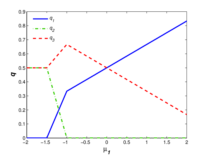
Therefore is not a substitutable choice model by Theorem 5.7. In fact, when we fix and plot the choice probabilities against in the range of values as shown in Figure 1, it is observed that increases in in the range of , i.e., alternative 3 is complementary to alternative 1 in that interval.
In addition to the quadratic example above, we can also easily generate a non-substitutable choice model through a proper choice welfare function :
Example 5.11
Consider the following function:
It is easy to see that is monotone, translation invariant and convex, therefore it is a choice welfare function. Also, it is differentiable. The corresponding choice probability is:
Furthermore, the second-order derivative of with respect to and is
It is positive if and only if . Therefore, under this choice model, when is large enough (compared to and ), then alternatives and will exhibit complementarity. On the other hand, if or (or both) are comparable to , then they will exhibit substitutability. Now we give a plausible explanation for this model. Suppose as in Example 1, we explain as the number of positive reviews for each product. Then the above substitutability pattern could be reasonable if alternatives and are both from some relatively unknown brand (which has very few positive reviews in the history), while alternative is from a well-known brand (which in contrast, has a lot of positive reviews). Then a few more positive reviews on either alternative or will be likely to positively impact the purchase probability of the other one, since it increases the overall attractiveness of this brand. On the other hand, if alternatives and have already gained enough positive reviews in the past, then further increasing the number of positive reviews of one of them will be more likely to attract the demand from the other one, rather than from alternative .
To numerically illustrate the above model, we fix , and plot the choice probability of alternative as a function of in the range of in Figure 2. From Figure 2, we can see that alternative is complementary to alternative when .

The above two examples show that by using the welfare-based framework, it is possible to construct choice models with more versatile substitution patterns. In addition, the above two examples further verify that even when , we can construct choice models that do not have a random utility representation (remember all random utility models are substitutable choice models). Therefore, the welfare-based choice model (thus also the representative agent model and the semi-parametric models) strictly subsumes the random utility model, even for . This result is an extension of the result obtained by Hofbauer and Sandholm (2002), which only showed the result for .
6 Constructing New Choice Models from Existing Ones
In this section, we show that by using the welfare-based choice model framework, one can easily construct new choice models from existing ones. In particular, we provide three transformations below by which new choice models can be derived from existing ones. In the following discussions, we use to denote existing welfare-based choice models with choice welfare function , and use and to denote the choice probability and the choice welfare function of the new model, respectively.
- 1.
Scaling. Given any existing choice welfare function and any , one can easily verify that is still a choice welfare function. The corresponding choice model is . We note that if has an RUM representation, then also has an RUM representation with . As becomes larger, the difference among is smaller and the choice will be more evenly distributed. As pointed out in Gigerenzer and Selten (2002), such can be used to model the level of rationality of the individual.
- 2.
Mixing. Let be a cover of , i.e., . Let be the choice welfare function on alternatives in , with choice probabilities . Define
where , . We can verify that is a choice welfare function and its corresponding choice model is
If has an RUM representation for all , then also has an RUM representation by assuming has a mixed distribution of , each with probability . This model can be used to model choice scenarios where there are different segments of customers. Customers of different segments may only care about a subset of the products and choose according to a certain choice model. Then the mixed model is the choice model for the entire population.
- 3.
Crossing. Let be an matrix with and , where refers to an -dimensional column vector of ones. Given an existing choice welfare function and its choice probabilities , we can easily verify that
is still a choice welfare function and the corresponding welfare-based choice model is
An example of such a transformation was in fact shown in Example 5.11, where is an MNL model for alternatives with and
In light of this example, we note that RUM is not closed under cross-transformation, i.e., even if has an RUM representation, may not. Thus, the cross-transformation provides us a way of generating new choice models.
7 Conclusion
In this paper, we proposed a new framework for discrete choice models: the welfare-based choice model, which is based on the idea of considering the expected utility an individual can get when facing a set of alternatives. We showed that the welfare-based choice model is equivalent to the representative agent model and the semi-parametric model, thus establishing the equivalence between the latter two. We also showed that the welfare-based choice model subsumes the random utility model by relaxing its requirement on properties of higher-order cross-partial derivatives of the choice welfare function. In particular, we showed that when there are only two alternatives, the welfare-based choice model is equivalent to the random utility model. We defined a new concept for choice models – substitutability and complementarity – and showed that under the new framework, we can construct choice models with complementary alternatives, thus enabling us to capture new choice patterns. We believe that this framework is useful for future studies of choice models.
References
- Ahipasaoglu et al. (2013) Ahipasaoglu, S. D., X. Li, K. Natarajan. 2013. A convex optimization approach for computing correlated choice probabilities with many alternatives. Working paper.
- Alptekinoglu and Temple (2013) Alptekinoglu, A., J. Temple. 2013. The exponomial choice model: A new alternative for assortment and price optimization. Working paper.
- Anderson et al. (1988) Anderson, S. P., A. De Palma, J. F. Thisse. 1988. A representative customer theory of the logit model. International Economic Review 29(3) 461–466.
- Anderson et al. (1992) Anderson, S. P., A. De Palma, J. F. Thisse. 1992. Discrete Choice Theory of Product Differentiation. The MIT Press.
- Ben-Akiva and Lerman (1985) Ben-Akiva, M., S. R. Lerman. 1985. Discrete Choice Analysis: Theory and Application to Travel Demand. The MIT Press.
- Bertsekas (2003) Bertsekas, D. 2003. Convex Analysis and Optimization. Athena Scientific.
- Blanchet et al. (2013) Blanchet, J., G. Gallego, V. Goyal. 2013. A Markov chain approximation to choice modeling. Working paper.
- Daganzo (1980) Daganzo, C. 1980. Multinomial Probit: The Theory and Its Application to Demand Forecasting. Academic Press.
- Farias et al. (2013) Farias, V. F., S. Jagabathula, D. Shah. 2013. A nonparametric approach to modeling choice with limited data. Management Science 59(2) 305–322.
- Gallego et al. (2014) Gallego, G., R. Ratliff, S. Shebalov. 2014. A general attraction model and sales-based linear program for network revenue management under customer choice. Operations Research .
- Gigerenzer and Selten (2002) Gigerenzer, G., R. Selten. 2002. Bounded Rationality: The Adaptive Toolbox. The MIT Press.
- Hofbauer and Sandholm (2002) Hofbauer, J., W. H. Sandholm. 2002. On the global convergence of stochastic fictitious play. Econometrica 70(6) 2265–2294.
- Jagabathula and Rusmevichientong (2013) Jagabathula, S., P. Rusmevichientong. 2013. A two-stage model of consideration set and choice: Learning, revenue prediction, and applications. Working paper.
- Mankiw (1997) Mankiw, G. 1997. Principles of Microeconomics. Cengage Learning.
- Mas-Colell et al. (1995) Mas-Colell, A., M. D. Whinston, J. R. Green. 1995. Microeconomic Theory. Oxford University Press.
- McFadden (1974) McFadden, D. 1974. Conditional logit analysis of qualitative choice behavior. P. Zarembka, ed., Frontiers in Econometrics. Academic Press, 105–142.
- McFadden (1980) McFadden, D. 1980. Econometric models for probabilistic choice among products. The Journal of Business 53(3) 13–29.
- McFadden and Train (2000) McFadden, D., K. Train. 2000. Mixed MNL models for discrete responses. Journal of Applied Econometrics 15 447–470.
- McFadden et al. (1978) McFadden, Daniel, et al. 1978. Modelling the choice of residential location. Institute of Transportation Studies, University of California.
- Mishra et al. (2014) Mishra, V. K., K. Natarajan, D. Padmanabhan, C.-P. Teo, X. Li. 2014. On theoretical and empirical aspects of marginal distribution choice models. Management Science 60(6) 1511–1531.
- Mishra et al. (2012) Mishra, V. K., K. Natarajan, H. Tao, C.-P. Teo. 2012. Choice prediction with semidefinite optimization when utilities are correlated. IEEE Transactions on Automatic Control 57(10) 2450–2463.
- Murota (2003) Murota, K. 2003. Discrete Convex Analysis. Society for Industrial and Applied Mathematics.
- Natarajan et al. (2009) Natarajan, K., M. Song, C.-P. Teo. 2009. Persistency model and its applications in choice modeling. Management Science 55(3) 453–469.
- Norets and Takahashi (2013) Norets, A., S. Takahashi. 2013. On the surjectivity of the mapping between utilities and choice probabilities. Quantitative Economics 4(1) 149–155.
- Rockafellar (1974) Rockafellar, T. 1974. Conjugate Duality and Optimization. Society for Industrial and Applied Mathematics.
- Simchi-Levi et al. (2014) Simchi-Levi, D., X. Chen, J. Bramel. 2014. Convexity and supermodularity. The Logic of Logistics. Springer, 15–44.
- Thurstone (1927) Thurstone, L. 1927. A law of comparative judgment. Psychological Review 34(4) 273–286.
- Train (2009) Train, K. E. 2009. Discrete Choice Methods with Simulation. Cambridge University Press.
Appendix
Proof of Theorem 3.6: The equivalence between 1 and 3 directly follows from Theorem 1. Next we show that . If is a differentiable choice welfare function, by Theorem 3.2, we know that
where . Therefore, is the convex conjugate of . By Theorem 6.3 in Rockafellar (1974), we know that is essentially differentiable if and only if is essentially strictly convex. Also, from the envelope theorem (see Mas-Colell et al. 1995),
where . Therefore,
Last, we show that . Given an essentially strictly convex , by Theorem 3.2, we know that
is a choice welfare function. Again, by Theorem 6.3 in
Rockafellar (1974), we know that is essentially
differentiable. Moreover, in our case, is a convex and
finitely valued function in , thus essentially
differentiability is equivalent to differentiability. Again, by
applying the envelope theorem, .
Therefore the theorem is proved.
Proof of Theorem 3.9: First we show the equivalence between 1 and 2. Based on Theorem 3.6, it suffices to prove that is superlinear if and only if defined by is upper bounded. If is superlinear, we have, for any ,
By reorganizing terms, we have
Therefore, , i.e., is upper bounded.
To show the other direction, if is upper bounded by a constant , then we have
i.e., is superlinear. Therefore, the equivalence between 1 and 2 is proved.
Next we show the equivalence between 1 and 3. We first show that for any superlinear differentiable choice welfare function , we can find a distribution set consisting of only distributions with finite expectation such that can be represented as
First, since is convex with , we have
| (23) |
where . Now we define a distribution set that is slightly different from that of Theorem 3.2. Specifically, let , where is an -point distribution with , . (Note that by the monotonicity and the translation invariance properties, must satisfy and .) Here,
where
| (25) |
with
| (26) |
Since , for all , we have Therefore,
Next we show that:
For any given , define (we break ties arbitrarily). There are two cases:
- 1.
For all such that , . In this case, we have
in which the last inequality is because of the convexity of .
- 2.
There exists some such that , but In this case, from the construction of , we have
where the first inequality follows from the fact that and , the second inequality is because of the definition of and the last inequality follows from the definition of superlinear function.
Based on the analysis of these two cases, we have
Then by equation (23) we have
Therefore, we have proved that statement 1 implies statement 3.
Finally, we prove that statement 3 implies statement 1. Suppose there exists a distribution such that for then for we have
Therefore we can conclude that is superlinear.
It remains to prove the last statement. We show that for any
there exists such that . Fix , we consider
| (27) |
Clearly, , since is a feasible solution. Moreover, since is translation invariant, we can restrict the feasible region of (27) to . For all , we have for some . Thus
However, by superlinearity of , we have:
Thus, for all , we have:
Let . In
order for to be optimal to (27), by the
above arguments, we would have for all . Thus we
can further restrict the feasible set of (27) to
, which is a compact set. Since is continuous, there
exists that attains maximum in problem
(27). By the first-order necessary condition,
This concludes the proof.
Proof of Proposition 5.3: Since is convex and differentiable, for any and any , we have
From these two inequalities, we have , for all and . Thus, alternative is complementary to itself.
Furthermore, if is second-order continuously
differentiable, then we have . Thus, if alternative is substitutable
(complementary, resp.) to alternative at
, then alternative is substitutable (complementary, resp.) to alternative at .
Proof of Theorem 5.7: In this proof, we use the following lemma from Murota (2003).
Lemma 7.1
Let be a function such that there exists at least one such that . Let be the convex conjugate of . We have
- 1.
If is submodular, then is supermodular.
- 2.
If and is supermodular, then is submodular.
Now we use this lemma to prove the theorem. To prove the first part, by Simchi-Levi et al. (2014), a differentiable function is submodular in if and only if is decreasing in for all . By the definition of , the result holds.
For the second part, let be the convex conjugate of . From Theorem 3.6, is essentially strictly convex and
For any and , define . Also define , then we have
where the second equality is due to the translation invariance property of . The submodularity of implies the submodularity of for all . Thus , as the convex conjugate of , is supermodular by Lemma 7.1.
For the last statement, since is an essentially strictly convex function, is well-defined. By Theorem 3.6, where . For any and , define . Also define , then we have
where the third equality holds since for all . From Lemma 7.1, given that and thus , is submodular. It remains to show that is also submodular. According to Theorem 5.7, it suffices to show that is locally decreasing with for all for all . Fix and let . We assume without loss of generality. We have from translation invariance property. But is non-decreasing with due to the submodularity of . Thus is submodular and is a substitutable choice model.
Proof of Theorem 5.8: We first consider the case where is differentiable for all . Let be the Lagrangian multiplier of the constraint . The KKT conditions (see Bertsekas 2003) for problem (20) can be written as:
Now we consider any two points and where is a unit vector along the -th coordinate axis and . Suppose that there exists a such that . Since is strictly convex, . There are two possible cases for :
- •
: In this case, we have and , therefore, we have .
- •
: In this case, , which implies that . But , we have .
In both cases, . This implies that for all . Note that we also have by Proposition 5.3. Therefore, we have , which contradicts with that . Thus we have for all . Since this is true for all and , is substitutable.
If is not differentiable, we need to replace the derivative with the subgradient in the above argument. Since is strictly convex, for all and if , the above argument is still valid.
Proof of Theorem 5.9: For , is an variate quadratic function. Let denote the Hessian matrix of . For and , the off-diagonal element , where
Thus, is supermodular if and only if for all and , which is equivalent to for all distinct .