跳到论文正文
W Papers独立论文阅读器 arXiv:1503.01837 论文正文 计算阅读时间 · 0%
引用这篇论文根据当前论文元数据生成,正式投稿前建议核对。


License: arXiv.org perpetual non-exclusive license
arXiv:1503.01837v1 [cs.CG] 06 Mar 2015

Combinatorial rigidity and independence of generalized pinned subspace-incidence constraint systems

Menghan Wang    Meera Sitharam
Abstract

Given a hypergraph HH with mm hyperedges and a set XX of mm pins, i.e. globally fixed subspaces in Euclidean space ℝd\mathbb{R}^{d}, a pinned subspace-incidence system is the pair (H,X)(H,X), with the constraint that each pin in XX lies on the subspace spanned by the point realizations in ℝd\mathbb{R}^{d} of vertices of the corresponding hyperedge of HH. We are interested in combinatorial characterization of pinned subspace-incidence systems that are minimally rigid, i.e. those systems that are guaranteed to generically yield a locally unique realization. As is customary, this is accompanied by a characterization of generic independence as well as rigidity.

In a previous paper [13], we used pinned subspace-incidence systems towards solving the fitted dictionary learning problem, i.e. dictionary learning with specified underlying hypergraph, and gave a combinatorial characterization of minimal rigidity for a more restricted version of pinned subspace-incidence system, with HH being a uniform hypergraph and pins in XX being 1-dimension subspaces. Moreover in a recent paper [2], the special case of pinned line incidence systems was used to model biomaterials such as cellulose and collagen fibrils in cell walls. In this paper, we extend the combinatorial characterization to general pinned subspace-incidence systems, with HH being a non-uniform hypergraph and pins in XX being subspaces with arbitrary dimension. As there are generally many data points per subspace in a dictionary learning problem, which can only be modeled with pins of dimension larger than 11, such an extension enables application to a much larger class of fitted dictionary learning problems.

1 Introduction

A pinned subspace-incidence system (H,X)(H,X) is an incidence constraint system specified as a hypergraph HH together with a set XX of subspaces or pins in ℝd\mathbb{R}^{d} in one-to-one correspondence with the hyperedges of HH. A realization of (H,X)(H,X) assigns points in ℝd\mathbb{R}^{d} to the vertices of HH, thereby subspaces to the hyperedges of HH. The subspace in ℝd\mathbb{R}^{d} corresponding to a hyperedge of HH contains the associated pin from XX. We are interested in characterization of pinned subspace-incidence systems that are minimally rigid, i.e. those systems that are guaranteed to generically yield a locally unique realization.

In a previous paper [13], we used pinned subspace-incidence systems towards solving fitted dictionary learning problems, i.e. dictionary learning with specified underlying hypergraphs. Dictionary learning (aka sparse coding) is the problem of obtaining a set dictionary vectors that sparsely represent a set of given data points in ℝd\mathbb{R}^{d}. Geometrically, such a sparse representation can be viewed as a subspace arrangement spanned by the dictionary vectors that contains all the data points. In fitted dictionary learning, the underlying hypergraph HH of the subspace arrangement is specified, and the problem becomes a pinned subspace-incidence systems with the pins corresponding to the span of data points on each subspace.

Moreover in a recent paper [2], we have used pinned subspace-incidence systems in modeling biomaterials such as cross-linking cellulose and collagen microfibrils in cell walls [3, 4, 14]. In such materials, each fibril is attached to some fixed larger organelle/membrane at one site, and cross-linked at two locations with other fibrils. Consequently, they can be modeled using a pinned line-incidence system with HH being a graph, where each fibril is modeled as an edge of HH with the two cross-linkings as its two vertices, and the attachment is modeled as the corresponding pin.

We gave in [13] a combinatorial characterization of minimal rigidity for a restricted version of pinned subspace-incidence system, with the underlying hypergraph HH being a uniform hypergraph and pins in XX being 1-dimension subspaces.

2 Contributions

In this paper, we extend the combinatorial characterization of minimal rigidity to general pinned subspace-incidence systems, where HH can be any non-uniform hypergraph, and each pin in XX is a subspace with arbitrary dimension. Such an extension enables application to a much larger class of fitted dictionary learning problems, since there are generally many data points per subspace in a dictionary learning problem, which can only be modeled with pins of dimension larger than 11.

As in our previous paper [13], we apply the classic method of White and Whiteley [18] to combinatorially characterize the rigidity of general pinned subspace-incidence systems. The primary technique is using the Laplace decomposition of the rigidity matrix, which corresponds to a map-decomposition [15] of the underlying hypergraph. The polynomial resulting from the Laplace decomposition is called the pure condition, which characterizes the conditions that the framework has to avoid for the combinatorial characterization to hold.

Previous works on related types of geometric constraint frameworks include pin-collinear body-pin frameworks [9], direction networks [20], slider-pinning rigidity [16], body-cad constraint system [8], kk-frames [18, 19], and affine rigidity [6]. However, we are not aware of any previous results on systems that are similar to pinned subspace-incidence systems.

3 Preliminaries

In this section, we introduce the formal definition of pinned subspace-incidence systems and basic concepts in combinatorial rigidity.

A hypergraph H=(V,E)H=(V,E) is a set VV of vertices and a set EE of hyperedges, where each hyperedge is a subset of VV. The rank r⁡(H)r(H) of a hypergraph HH is the maximum cardinality of any edge in EE, i.e. r⁡(H)=maxek∈E⁡s⁡(ek)r(H)=\max_{e_{k}\in E}s(e_{k}), where s⁡(ek)s(e_{k}) denotes the cardinality of the hyperedge eke_{k}. A hypergraph is ss-uniform if all edges in EE have the same cardinality ss. A configuration or realization of a hypergraph H=(V,E)H=(V,E) in ℝd\mathbb{R}^{d} is a mapping of points in ℝd\mathbb{R}^{d} to the vertices of HH, p:V→ℝdp:V\rightarrow\mathbb{R}^{d}. When there is no ambiguity, we simply use pip_{i} to denote the point p⁡(vi)p(v_{i}), p⁡(ek)p(e_{k}) to denote the set of points {p⁡(vi)|vi∈ek}\{p(v_{i})|v_{i}\in e_{k}\}, and sks_{k} to denote the cardinality s⁡(ek)s(e_{k}).

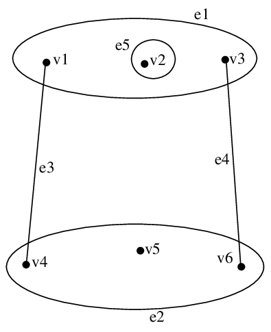
An example of a rank-3 hypergraph is given in Figure 1(a).
Refer to caption
(a)
Refer to caption
(b)
Figure 1: (a) A rank-3 non-uniform hypergraph with 6 vertices and 5 edges, where s1=s2=3s_{1}=s_{2}=3, s3=s4=2s_{3}=s_{4}=2, s5=1s_{5}=1. (b) A pinned subspace-incidence framework in d=4d=4 (projectivized in ℙ3​(ℝ)\mathbb{P}^{3}(\mathbb{R})) on the hypergraph from (a), with m1=m3=2m_{1}=m_{3}=2, m2=3m_{2}=3, m4=m5=1m_{4}=m_{5}=1, where the crosses on each hyperedge represent points spanning the associated pin.

In the following, we use ⟨S⟩\langle S\rangle to denote the subspace spanned by a set SS of points in ℝd\mathbb{R}^{d}.

Definition 1 (Pinned Subspace-Incidence System).

A pinned subspace-incidence system in ℝd\mathbb{R}^{d} is a pair (H,X)(H,X), where H=(V,E,m)H=(V,E,m) is a weighted hypergraph with hyperedges of rank r⁡(H)<dr(H)<d, and X={x1,x2,…,x|E|}X=\{x_{1},x_{2},\ldots,x_{|E|}\} is a set of pins (subspaces of ℝd\mathbb{R}^{d}) in one-to-one correspondence with the hyperedges of HH. Here the weight assignment is a function m:E⁡(H)→ℤ+m:E(H)\rightarrow\mathbb{Z}^{+}, where m⁡(e)m(e) denotes the dimension of the pin associated with the hyperedge ee. Often we ignore the weight mm and just refer to the hypergraph (V,E)(V,E) as HH.

A pinned subspace-incidence framework realizing the pinned subspace-incidence system (H,X)(H,X) is a triple (H,X,p)(H,X,p), where pp is a realization of HH, such that for all pins xk∈Xx_{k}\in X, xkx_{k} is contained in ⟨p⁡(ek)⟩\langle p(e_{k})\rangle, the subspace spanned by the set of points realizing the vertices of the hyperedge eie_{i} corresponding to xkx_{k}.

We may write m⁡(xk)m(x_{k}) or simply mkm_{k} in substitute of m⁡(ek)m(e_{k}), where xkx_{k} is the pin associated with the hyperedge eke_{k}.

Since we only care about incidence relations, we projectivize the Euclidean space ℝd\mathbb{R}^{d} to treat the pinned subspace-incidence system in the real projective space ℙd−1​(ℝ)\mathbb{P}^{d-1}(\mathbb{R}), and use the same notation for the pins and hypergraph realization when the meaning is clear from the context.

Figure 1(b) gives an example of a pinned subspace-incidence framework in the projective space ℙd−1​(ℝ)\mathbb{P}^{d-1}(\mathbb{R}) with d=4d=4, where each pin is the subspace spanned by the set of cross-denoted points on the corresponding hyperedge.

Definition 2.

A pinned subspace-incidence system (H,X)(H,X) is independent if none of the algebraic constraints is in the ideal generated by others, which generically implies the existence of a realization. It is rigid if there exist at most finitely many realizations. It is minimally rigid if it is both rigid and independent. It is globally rigid if there exits at most one realization.

4 Algebraic Representation and Linearization

In the following, we use A⁡[R,C]A[R,C] to denote a submatrix of a matrix AA, where RR and CC are respectively index sets of the rows and columns contained in the submatrix. In addition, A⁡[R,⋅]A[R,{\scalebox{1.25}{$\,\cdot\,$}}] represents the submatrix containing row set RR and all columns, and A⁡[⋅,C]A[{\scalebox{1.25}{$\,\cdot\,$}},C] represents the submatrix containing column set CC and all rows.

4.1 Algebraic Representation

A pin xkx_{k} associated with a hyperedge ek={v1k,v2k,…,vskk}e_{k}=\{v^{k}_{1},v^{k}_{2},\ldots,v^{k}_{s_{k}}\} of cardinality sks_{k} is constrained to be contained in the subspace ⟨p⁡(ek)⟩\langle p(e_{k})\rangle spanned by the point set {p1k,p2k,…,pskk}\{p^{k}_{1},p^{k}_{2},\ldots,p^{k}_{s_{k}}\}. As xkx_{k} is a subspace of dimension mk−1m_{k}-1 in ℙd−1​(ℝ)\mathbb{P}^{d-1}(\mathbb{R}), we can pick a set of mkm_{k} points {x1k,x2k,…,xmkk}\{x^{k}_{1},x^{k}_{2},\ldots,x^{k}_{m_{k}}\} spanning xkx_{k} from xkx_{k}. Now the constraint is equivalent to requiring each such point xlkx^{k}_{l} to lie on ⟨p⁡(e)⟩\langle p(e)\rangle, for 1≤l≤mk1\leq l\leq m_{k}. We call each such point xlkx^{k}_{l} a multipin as it acts like a pin with m⁡(xlk)=1m(x^{k}_{l})=1.

Using homogeneous coordinates pik=[pi,1kpi,2k…pi,d−1k]p^{k}_{i}=[\begin{array}[]{cccc}p^{k}_{i,1}&p^{k}_{i,2}&\ldots&p^{k}_{i,d-1}\end{array}] and xlk=[xl,1kxl,2k…xl,d−1k]x^{k}_{l}=[\begin{array}[]{cccc}x^{k}_{l,1}&x^{k}_{l,2}&\ldots&x^{k}_{l,d-1}\end{array}], we write this incidence constraint for each point xlx_{l} by letting all the sk×sks_{k}\times s_{k} minors of the sk×(d−1)s_{k}\times(d-1) matrix

Elk=[p1k−xlkp2k−xlk⋮pskk−xlk]E^{k}_{l}=\left[\begin{array}[]{c}p^{k}_{1}-x^{k}_{l}\\ p^{k}_{2}-x^{k}_{l}\\ \vdots\\ p^{k}_{s_{k}}-x^{k}_{l}\end{array}\right]

be zero. There are (d−1sk)d-1\choose s_{k} minors, giving (d−1sk)d-1\choose s_{k} equations. Note that any d−skd-s_{k} of these (d−1sk)d-1\choose s_{k} equations are independent and span the rest. So we can write the incidence constraint as (d−sk)(d-s_{k}) independent equations:

det(Elk​[⋅,C⁡(t)])=0,1≤t≤d−sk\det\left(E^{k}_{l}[{\scalebox{1.25}{$\,\cdot\,$}},C(t)]\right)=0,\qquad 1\leq t\leq d-s_{k} (1)

where C⁡(t)C(t) denote the following index sets of columns in EE:

C⁡(t)={1,2,…​sk−1}∪{sk−1+t}1≤t≤d−sC(t)=\{1,2,\ldots s_{k}-1\}\cup\{s_{k}-1+t\}\qquad 1\leq t\leq d-s

In other words, C⁡(t)C(t) contains the first sk−1s_{k}-1 columns together with Column sk−1+ts_{k}-1+t.

Now the incidence constraint for the pin xkx_{k} is represented as mk​(d−sk)m_{k}(d-s_{k}) equations for all the mkm_{k} multipins {x1k,x2k,…​xmkk}\{x^{k}_{1},x^{k}_{2},\ldots x^{k}_{m_{k}}\}. Consequently, the pinned subspace-incidence problem reduces to solving a system of ∑k=1|E|mk​(d−sk)\sum_{k=1}^{|E|}m_{k}(d-s_{k}) equations, each of form (1). We denote this algebraic system by (H,X)​(p)=0(H,X)(p)=0.

4.2 Genericity

We are interested in characterizing minimal rigidity of pinned subspace-incidence systems. However, checking independence relative to the ideal generated by the variety is computationally hard and best known algorithms, such as computing Gröbner basis, are exponential in time and space [11]. However, the algebraic system can be linearized at generic or regular (non-singular) points, whereby the independence and rigidity of the algebraic system (H,X)​(p)=0(H,X)(p)=0 reduces to linear independence and maximal rank at generic frameworks.

In algebraic geometry, a property being generic intuitively means that the property holds on the open dense complement of an (real) algebraic variety. Formally,

Definition 3.

A pinned subspace-incidence system (H,X)(H,X) is generic w.r.t. a property QQ if and only if there exists a neighborhood N⁡(X)N(X) such that for all systems (H,X′)(H,X^{\prime}) with X′∈N⁡(X)X^{\prime}\in N(X), (H,X′)(H,X^{\prime}) satisfies QQ if and only if (H,X)(H,X) satisfies QQ.

Similarly, a framework (H,X,p)(H,X,p) is generic w.r.t. a property QQ if and only if there exists a neighborhood N⁡(p)N(p) such that for all frameworks (H,X,q)(H,X,q) with q∈N⁡(p)q\in N(p), (H,X,q)(H,X,q) satisfies QQ if and only if (H,X,p)(H,X,p) satisfies QQ.

Furthermore we can define generic properties in terms of the underlying weighted hypergraph.

Definition 4.

A property QQ of pinned subspace-incidence systems is generic (i.e, becomes a property of the underlying weighted hypergraph alone) if for any weighted hypergraph H=(V,E,m)H=(V,E,m), either all generic (w.r.t. QQ) systems (H,X)(H,X) satisfies QQ, or all generic (w.r.t. QQ) systems (H,X)(H,X) do not satisfy QQ.

Once an appropriate notion of genericity is defined, we can treat QQ as a property of a hypergraph. The primary activity of the area of combinatorial rigidity is to give purely combinatorial characterizations of such generic properties QQ. In the process of drawing such combinatorial characterizations, the notion of genericity may have to be further restricted by so-called pure conditions that are necessary for the combinatorial characterization to go through (we will see this in the proof of Theorem 11).

4.3 Linearization as Rigidity Matrix

Next we follow the approach taken by traditional combinatorial rigidity theory [1, 7] to show that rigidity and independence (based on nonlinear polynomials) of pinned subspace-incidence systems are generically properties of the underlying weighted hypergraph HH, and can furthermore be captured by linear conditions in an infinitesimal setting. Specifically, Lemma 6 shows that rigidity of a pinned subspace-incidence system is equivalent to existence of a full rank rigidity matrix, obtained by taking the Jacobian of the algebraic system (H,X)​(p)(H,X)(p) at a regular point.

A rigidity matrix of a framework (H,X,p)(H,X,p) is a matrix whose kernel is the infinitesimal motions (flexes) of (H,X,p)(H,X,p). A framework is infinitesimally rigid if the space of infinitesimal motion is trivial, i.e. the rigidity matrix has full rank. To define a rigidity matrix for a pinned subspace-incidence framework (H,X,p)(H,X,p), we take the Jacobian of the algebraic system (H,X)​(p)=0(H,X)(p)=0 by taking partial derivatives with respect to the coordinates of pip_{i}’s. In the Jacobian, each vertex viv_{i} has d−1d-1 corresponding columns, and each pin xkx_{k} associated with the hyperedge ek={v1k,v2k,…,vskk}e_{k}=\{v^{k}_{1},v^{k}_{2},\ldots,v^{k}_{s_{k}}\} has mk​(d−sk)m_{k}(d-s_{k}) corresponding rows, where each equation det(Elk​[⋅,C⁡(t)])=0\det\left(E^{k}_{l}[{\scalebox{1.25}{$\,\cdot\,$}},C(t)]\right)=0 (1), i.e. Equation tt of the multipin xlkx^{k}_{l}, gives the following row (the columns corresponding to vertices not in eke_{k} are all zero):

[ 0,\displaystyle\bigg[\;0, …,0,0,∂det⁡(Elk​[⋅,C⁡(t)])∂p1,1k,∂det⁡(Elk​[⋅,C⁡(t)])∂p1,2k,…,∂det⁡(Elk​[⋅,C⁡(t)])∂p1,d−1k,0,0,\displaystyle\ldots,0,0,\frac{\partial\det\left(E^{k}_{l}[{\scalebox{1.25}{$\,\cdot\,$}},C(t)]\right)}{\partial p^{k}_{1,1}},\frac{\partial\det\left(E^{k}_{l}[{\scalebox{1.25}{$\,\cdot\,$}},C(t)]\right)}{\partial p^{k}_{1,2}},\ldots,\frac{\partial\det\left(E^{k}_{l}[{\scalebox{1.25}{$\,\cdot\,$}},C(t)]\right)}{\partial p^{k}_{1,d-1}},0,0,
…,0,0,∂det⁡(Elk​[⋅,C⁡(t)])∂p2,1k,∂det⁡(Elk​[⋅,C⁡(t)])∂p2,2k,…,∂det⁡(Elk​[⋅,C⁡(t)])∂p2,d−1k,0,0,…\displaystyle\ldots,0,0,\frac{\partial\det\left(E^{k}_{l}[{\scalebox{1.25}{$\,\cdot\,$}},C(t)]\right)}{\partial p^{k}_{2,1}},\frac{\partial\det\left(E^{k}_{l}[{\scalebox{1.25}{$\,\cdot\,$}},C(t)]\right)}{\partial p^{k}_{2,2}},\ldots,\frac{\partial\det\left(E^{k}_{l}[{\scalebox{1.25}{$\,\cdot\,$}},C(t)]\right)}{\partial p^{k}_{2,d-1}},0,0,\ldots
…​…\displaystyle\ldots\ldots
…,0,0,∂det⁡(Elk​[⋅,C⁡(t)])∂psk,1k,∂det⁡(Elk​[⋅,C⁡(t)])∂psk,2k,…,∂det⁡(Elk​[⋅,C⁡(t)])∂psk,d−1k,0,…,0]\displaystyle\ldots,0,0,\frac{\partial\det\left(E^{k}_{l}[{\scalebox{1.25}{$\,\cdot\,$}},C(t)]\right)}{\partial p^{k}_{s_{k},1}},\frac{\partial\det\left(E^{k}_{l}[{\scalebox{1.25}{$\,\cdot\,$}},C(t)]\right)}{\partial p^{k}_{s_{k},2}},\ldots,\frac{\partial\det\left(E^{k}_{l}[{\scalebox{1.25}{$\,\cdot\,$}},C(t)]\right)}{\partial p^{k}_{s_{k},d-1}},0,\ldots,0\;\bigg] (2)

Let VkV^{k} be the matrix whose rows are coordinates of p1k,p2k,…,pskkp^{k}_{1},p^{k}_{2},\ldots,p^{k}_{s_{k}}:

[p1,1p1,2…p1,d−1p2,1p2,2…p2,d−1⋮⋮⋱⋮psk,1psk,2…psk,d−1]\left[\begin{array}[]{cccc}p_{1,1}&p_{1,2}&\ldots&p_{1,d-1}\\ p_{2,1}&p_{2,2}&\ldots&p_{2,d-1}\\ \vdots&\vdots&\ddots&\vdots\\ p_{s_{k},1}&p_{s_{k},2}&\ldots&p_{s_{k},d-1}\end{array}\right]

Let VtkV^{k}_{t} be the Vk​[⋅,C​(t)]V^{k}[{\scalebox{1.25}{$\,\cdot\,$}},C(t)], i.e. the sk×sks_{k}\times s_{k} submatrix of VkV^{k} containing only columns in C⁡(t)C(t). Let Vt,jkV^{k}_{t,j} be the matrix obtained from VtkV^{k}_{t} by replacing the column corresponding to Coordinate jj with the all-ones vector (1,1,…,1)(1,1,\ldots,1) for j∈C⁡(t)j\in C(t), and the zero matrix for j∉C⁡(t)j\notin C(t). Let Dt,jkD^{k}_{t,j} be the determinant of Vt,jkV^{k}_{t,j}. Let xl=∑i=1skbik,l​vikx_{l}=\sum_{i=1}^{s_{k}}b^{k,l}_{i}v^{k}_{i} (note that ∑i=1skbik,l=1\sum_{i=1}^{s_{k}}b^{k,l}_{i}=1). Now (2) can be rewritten in the following simplified form:

rt,lk=[ 0,\displaystyle r^{k}_{t,l}=\Big[\;0,\, …, 0, 0,Dt,1k​b1k,l,Dt,2k​b1k,l,…,Dt,d−1k​b1k,l, 0, 0,\displaystyle\ldots,\,0,\,0,\,D^{k}_{t,1}b^{k,l}_{1},\,D^{k}_{t,2}b^{k,l}_{1},\,\ldots,\,D^{k}_{t,d-1}b^{k,l}_{1},\,0,\,0,\,
…, 0, 0,Dt,1k​b2k,l,Dt,2k​b2k,l,…,Dt,d−1k​b2k,l, 0, 0,…\displaystyle\ldots,\,0,\,0,\,D^{k}_{t,1}b^{k,l}_{2},\,D^{k}_{t,2}b^{k,l}_{2},\,\ldots,\,D^{k}_{t,d-1}b^{k,l}_{2},\,0,\,0,\,\ldots
…​…\displaystyle\ldots\ldots
…, 0, 0,Dt,1kbskk,l,Dt,2kbskk,l,…,Dt,d−1kbskk,l, 0, 0,…, 0]\displaystyle\ldots,\,0,\,0,\,D^{k}_{t,1}b^{k,l}_{s_{k}},\,D^{k}_{t,2}b^{k,l}_{s_{k}},\,\ldots,\,D^{k}_{t,d-1}b^{k,l}_{s_{k}},\,0,\,0,\,\ldots,\,0\;\Big] (3)

Each vertex vikv^{k}_{i} has the entries Dt,jk​bik,l,1≤j≤d−1D^{k}_{t,j}b^{k,l}_{i},1\leq j\leq d-1 in its d−1d-1 columns, among which exactly sks_{k} entries with j∈C⁡(t)j\in C(t), i.e. the first sk−1s_{k}-1 columns together with Column sk−1+ts_{k}-1+t, are generically non-zero. Note that the terms Dt,sk−1+tkD^{k}_{t,s_{k}-1+t} are equal for all tt, so we may just use DkD^{k} to denote it.

For each 1≤t≤d−sk1\leq t\leq d-s_{k}, there are mkm_{k} rows as (3), where each multipin xlkx^{k}_{l} corresponds to the row rt,lkr^{k}_{t,l} for 1≤l≤mk1\leq l\leq m_{k}. These mkm_{k} rows have exactly the same row pattern except for different bik,lb^{k,l}_{i}’s:

v1,1v1,2…v1,d−1vsk,1vsk,2…vsk,d−1…Dt,1k​b1k,1Dt,2k​b1k,1…Dt,d−1k​b1k,1……Dt,1k​bskk,1Dt,2k​bskk,1…Dt,d−1k​bskk,1……Dt,1k​b1k,2Dt,2k​b1k,2…Dt,d−1k​b1k,2……Dt,1k​bskk,2Dt,2k​bskk,2…Dt,d−1k​bskk,2…\BAmulticolumn​12​c​⋱…Dt,1k​b1k,mkDt,2k​b1k,mk…Dt,d−1k​b1k,mk……Dt,1k​bskk,mkDt,2k​bskk,mk…Dt,d−1k​bskk,mk…\hskip-50.0pt\begin{array}[]{*{12}{c}}&v_{1,1}&v_{1,2}&\ldots&v_{1,d-1}&&&v_{s_{k},1}&v_{s_{k},2}&\ldots&v_{s_{k},d-1}&\\ \ldots&D^{k}_{t,1}b^{k,1}_{1}&D^{k}_{t,2}b^{k,1}_{1}&\ldots&D^{k}_{t,d-1}b^{k,1}_{1}&\ldots&\ldots&D^{k}_{t,1}b^{k,1}_{s_{k}}&D^{k}_{t,2}b^{k,1}_{s_{k}}&\ldots&D^{k}_{t,d-1}b^{k,1}_{s_{k}}&\ldots\\ \ldots&D^{k}_{t,1}b^{k,2}_{1}&D^{k}_{t,2}b^{k,2}_{1}&\ldots&D^{k}_{t,d-1}b^{k,2}_{1}&\ldots&\ldots&D^{k}_{t,1}b^{k,2}_{s_{k}}&D^{k}_{t,2}b^{k,2}_{s_{k}}&\ldots&D^{k}_{t,d-1}b^{k,2}_{s_{k}}&\ldots\\ \BAmulticolumn{12}{c}{\ddots}\\ \ldots&D^{k}_{t,1}b^{k,m_{k}}_{1}&D^{k}_{t,2}b^{k,m_{k}}_{1}&\ldots&D^{k}_{t,d-1}b^{k,m_{k}}_{1}&\ldots&\ldots&D^{k}_{t,1}b^{k,m_{k}}_{s_{k}}&D^{k}_{t,2}b^{k,m_{k}}_{s_{k}}&\ldots&D^{k}_{t,d-1}b^{k,m_{k}}_{s_{k}}&\ldots\\ \end{array}
Example 1.

For d=4d=4, consider a pin xx with m⁡(x)=2m(x)=2 associated with the hyperedge e={v1,v2}e=\{v_{1},v_{2}\}. The pin has the following m⁡(x)⋅(d−s⁡(e))=4m(x)\cdot(d-s(e))=4 rows in the simplified Jacobian (the index kk is omitted):

v1,1v1,2v1,3v2,1v2,2v2,3t=1,l=1…D1,1​b11D​b110…D1,1​b21D​b210…t=1,l=2…D1,1​b12D​b120…D1,1​b22D​b220…t=2,l=1…D2,1​b110D​b11…D2,1​b210D​b21…t=2,l=2…D2,1​b120D​b12…D2,1​b220D​b22…\begin{array}[]{c@{\hspace{1.5em}}c@{\hspace{1.5em}}c@{\hspace{1.5em}}c@{\hspace{1.5em}}c@{\hspace{1.5em}}c@{\hspace{1.5em}}c@{\hspace{1.5em}}c@{\hspace{1.5em}}c@{\hspace{1.5em}}c@{\hspace{1.5em}}}\hfil\hskip 15.00002pt&\hfil\hskip 15.00002pt&v_{1,1}\hfil\hskip 15.00002pt&v_{1,2}\hfil\hskip 15.00002pt&v_{1,3}\hfil\hskip 15.00002pt&\hfil\hskip 15.00002pt&v_{2,1}\hfil\hskip 15.00002pt&v_{2,2}\hfil\hskip 15.00002pt&v_{2,3}\hfil\hskip 15.00002pt&\hfil\hskip 15.00002pt\\ t=1,l=1\hfil\hskip 15.00002pt&\quad\ldots\hfil\hskip 15.00002pt&D_{1,1}b^{1}_{1}\hfil\hskip 15.00002pt&Db^{1}_{1}\hfil\hskip 15.00002pt&0\hfil\hskip 15.00002pt&\ldots\hfil\hskip 15.00002pt&D_{1,1}b^{1}_{2}\hfil\hskip 15.00002pt&Db^{1}_{2}\hfil\hskip 15.00002pt&0\hfil\hskip 15.00002pt&\ldots\hfil\hskip 15.00002pt\\ t=1,l=2\hfil\hskip 15.00002pt&\quad\ldots\hfil\hskip 15.00002pt&D_{1,1}b^{2}_{1}\hfil\hskip 15.00002pt&Db^{2}_{1}\hfil\hskip 15.00002pt&0\hfil\hskip 15.00002pt&\ldots\hfil\hskip 15.00002pt&D_{1,1}b^{2}_{2}\hfil\hskip 15.00002pt&Db^{2}_{2}\hfil\hskip 15.00002pt&0\hfil\hskip 15.00002pt&\ldots\hfil\hskip 15.00002pt\\ t=2,l=1\hfil\hskip 15.00002pt&\quad\ldots\hfil\hskip 15.00002pt&D_{2,1}b^{1}_{1}\hfil\hskip 15.00002pt&0\hfil\hskip 15.00002pt&Db^{1}_{1}\hfil\hskip 15.00002pt&\ldots\hfil\hskip 15.00002pt&D_{2,1}b^{1}_{2}\hfil\hskip 15.00002pt&0\hfil\hskip 15.00002pt&Db^{1}_{2}\hfil\hskip 15.00002pt&\ldots\hfil\hskip 15.00002pt\\ t=2,l=2\hfil\hskip 15.00002pt&\quad\ldots\hfil\hskip 15.00002pt&D_{2,1}b^{2}_{1}\hfil\hskip 15.00002pt&0\hfil\hskip 15.00002pt&Db^{2}_{1}\hfil\hskip 15.00002pt&\ldots\hfil\hskip 15.00002pt&D_{2,1}b^{2}_{2}\hfil\hskip 15.00002pt&0\hfil\hskip 15.00002pt&Db^{2}_{2}\hfil\hskip 15.00002pt&\ldots\hfil\hskip 15.00002pt\\ \end{array}

We define the rigidity matrix M⁡(H,X,p)M(H,X,p) or simply M⁡(p)M(p) for a pinned subspace-incidence framework (H,X,p)(H,X,p) to be the simplified Jacobian matrix obtained above, where each row has form (3). It is a matrix of size ∑kmk​(d−sk)\sum_{k}m_{k}(d-s_{k}) by n⁡(d−1)n(d-1).

Definition 5.

A pinned subspace-incidence framework (H,X,p)(H,X,p) and the corresponding system (H,X)(H,X) is generic if pp and XX are regular/non-singular points with respect to the algebraic system (H,X)​(p)=0(H,X)(p)=0.

We use M⁡(H)M(H) of simply MM to denote the generic rigidity matrix for a weighted hypergraph HH. Note that the rank of MM cannot be less than the rank of M⁡(p)M(p) for any specific realization pp.

Lemma 6.

Generic infinitesimal rigidity of a pinned subspace-incidence framework (H,X,p)(H,X,p) is equivalent to generic rigidity of the system (H,X)(H,X).

The proof of Lemma 6 follows the traditional combinatorial rigidity approach [1] and is given in the Appendix.

5 Combinatorial rigidity characterization

5.1 Required hypergraph properties

This section introduces pure hypergraph properties and definitions that will be used in stating and proving our main theorem.

Definition 7.

A hypergraph H=(V,E)H=(V,E) is (k,0)(k,0)-sparse if for any V′⊂V{V^{\prime}}\subset V, the induced subgraph H′=(V′,E′){H^{\prime}}=({V^{\prime}},{E^{\prime}}) satisfies |E′|≤k​|V′||{E^{\prime}}|\leq k|{V^{\prime}}|. A hypergraph HH is (k,0)(k,0)-tight if HH is (k,0)(k,0)-sparse and |E|=k​|V||E|=k|V|.

This is a special case of the (k,l)(k,l)-sparsity condition that was formally studied widely in the geometric constraint solving and combinatorial rigidity literature before it was given a name in [10]. A relevant concept from graph matroids is map-graph, defined as follows.

Definition 8.

An orientation of a hypergraph is given by identifying as the tail of each edge one of its endpoints. The out-degree of a vertex is the number of edges which identify it as the tail and connect vv to V−vV-v. A map-graph is a hypergraph that admits an orientation such that the out degree of every vertex is exactly one.

The following lemma from [15] follows Tutte-Nash Williams [17, 12] to give a useful characterization of (k,0)(k,0)-tight graphs in terms of maps.

Lemma 9.

A hypergraph HH is composed of kk edge-disjoint map-graphs if and only if HH is (k,0)(k,0)-tight.

Our characterization of rigidity of a weighted hypergraph HH is based on map-decomposition of a multi-hypergraph H^\hat{H} obtained from HH.

Definition 10.

Given a weighted hypergraph H=(V,E,m)H=(V,E,m), the associated multi-hypergraph H^=(V,E^)\hat{H}=(V,\hat{E}) is obtained by replacing each hyperedge eke_{k} in EE with a set Ek{E}^{k} of mk​(d−sk)m_{k}(d-s_{k}) copies of multi-hyperedges.

A labeling of a multi-hypergraph H^\hat{H} gives a one-to-one correspondence between EkE^{k} and the set RkR^{k} of mk​(d−sk)m_{k}(d-s_{k}) rows for the hyperedge eke^{k} in the rigidity matrix MM, where the multi-hyperedge corresponding to the row rt,lkr^{k}_{t,l} is labeled et,lke^{k}_{t,l}.

5.2 Characterizing rigidity

In this section, we apply [18] to give combinatorial characterization for minimal rigidity of pinned subspace-incidence systems.

Theorem 11 (Main Theorem).

A pinned subspace-incidence system is generically minimally rigid if and only if:

  1. 1.

    The underlying weighted hypergraph H=(V,E,m)H=(V,E,m) satisfies ∑k=1|E|mk​(d−sk)=(d−1)​|V|\sum_{k=1}^{|E|}m_{k}(d-s_{k})=(d-1)|V|, and ∑ek∈E′mk​(d−sk)≤(d−1)​|V′|\sum_{e_{k}\in E^{\prime}}m_{k}(d-s_{k})\leq(d-1)|V^{\prime}| for every vertex induced subgraph H′=(V′,E′)H^{\prime}=(V^{\prime},E^{\prime}). In other words, the associated multi-hypergraph H^=(V,E^)\hat{H}=(V,\hat{E}) has a decomposition into (d−1)(d-1) maps.

  2. 2.

    There exists a labeling of H^\hat{H} compatible with the map-decomposition (defined later) such that in each set EkE^{k} of multi-hyperedges,

    (a) two multi-hyperedges et1,l1ke^{k}_{t_{1},l_{1}} and et2,l2ke^{k}_{t_{2},l_{2}} with l1=l2l_{1}=l_{2} are not contained in the same map in the map-decomposition,

    (b) two multi-hyperedges et1,l1ke^{k}_{t_{1},l_{1}} and et2,l2ke^{k}_{t_{2},l_{2}} with t1=t2t_{1}=t_{2} do not have the same vertex as tail in the map-decomposition.

To prove Theorem 11, we apply Laplace expansion to the determinant of the rigidity matrix MM, which corresponds to decomposing the (d−1,0)(d-1,0)-tight multi-hypergraph H^\hat{H} as a union of d−1d-1 maps. We then prove det(M)\det(M) is not identically zero by showing that the minors corresponding to each map are not identically zero, as long as a certain polynomial called pure condition is avoided by the framework. The pure condition characterizes the non-genericity that the framework has to avoid in order for the combinatorial characterization to go through: see Example 4.

A Laplace expansion rewrites the determinant of the rigidity matrix MM as a sum of products of determinants (brackets) representing each of the coordinates taken separately. In order to see the relationship between the Laplace expansion and the map-decomposition, we first group the columns of MM into d−1d-1 column groups CjC_{j} according to the coordinates, where columns for the first coordinate of each vertex belong to C1C_{1}, columns for the second coordinate of each vertex belong to C2C_{2}, etc.

Example 2.

For d=4d=4, consider a pin xx with m⁡(x)=2m(x)=2 associated with the hyperedge e=v1,v2e={v_{1},v_{2}}. The regrouped rigidity matrix has d−1=3d-1=3 column groups, where the pin xx has the following 44 rows (the index kk is omitted):

v1,1v2,1v1,2v2,2v1,3v2,3t=1,l=1…D1,1​b11…D1,1​b21……D​b11…D​b21…t=1,l=2…D1,1​b12…D1,1​b22……D​b12…D​b22…t=2,l=1…D2,1​b11…D2,1​b21……D​b11…D​b21…t=2,l=2…D2,1​b12…D2,1​b22……D​b12…D​b22…\hskip-30.0pt\begin{array}[]{c@{\hspace{0.8em}}c@{\hspace{0.8em}}c@{\hspace{0.8em}}c@{\hspace{0.8em}}c@{\hspace{0.8em}}c@{\hspace{0.8em}}c@{\hspace{0.8em}}c@{\hspace{0.8em}}c@{\hspace{0.8em}}c@{\hspace{0.8em}}c@{\hspace{0.8em}}c@{\hspace{0.8em}}c@{\hspace{0.8em}}c@{\hspace{0.8em}}c@{\hspace{0.8em}}c@{\hspace{0.8em}}}\hfil\hskip 8.00003pt&\hfil\hskip 8.00003pt&v_{1,1}\hfil\hskip 8.00003pt&\hfil\hskip 8.00003pt&v_{2,1}\hfil\hskip 8.00003pt&\hfil\hskip 8.00003pt&\hfil\hskip 8.00003pt&v_{1,2}\hfil\hskip 8.00003pt&\hfil\hskip 8.00003pt&v_{2,2}\hfil\hskip 8.00003pt&\hfil\hskip 8.00003pt&\hfil\hskip 8.00003pt&v_{1,3}\hfil\hskip 8.00003pt&\hfil\hskip 8.00003pt&v_{2,3}\hfil\hskip 8.00003pt&\hfil\hskip 8.00003pt\\ t=1,l=1\hfil\hskip 8.00003pt&\>\;\ldots\hfil\hskip 8.00003pt&D_{1,1}b^{1}_{1}\hfil\hskip 8.00003pt&\ldots\hfil\hskip 8.00003pt&D_{1,1}b^{1}_{2}\hfil\hskip 8.00003pt&\ldots\hfil\hskip 8.00003pt&\ldots\hfil\hskip 8.00003pt&Db^{1}_{1}\hfil\hskip 8.00003pt&\ldots\hfil\hskip 8.00003pt&Db^{1}_{2}\hfil\hskip 8.00003pt&\ldots\hfil\hskip 8.00003pt&\hfil\hskip 8.00003pt&\hfil\hskip 8.00003pt&\hfil\hskip 8.00003pt&\hfil\hskip 8.00003pt&\hfil\hskip 8.00003pt\\ t=1,l=2\hfil\hskip 8.00003pt&\>\;\ldots\hfil\hskip 8.00003pt&D_{1,1}b^{2}_{1}\hfil\hskip 8.00003pt&\ldots\hfil\hskip 8.00003pt&D_{1,1}b^{2}_{2}\hfil\hskip 8.00003pt&\ldots\hfil\hskip 8.00003pt&\ldots\hfil\hskip 8.00003pt&Db^{2}_{1}\hfil\hskip 8.00003pt&\ldots\hfil\hskip 8.00003pt&Db^{2}_{2}\hfil\hskip 8.00003pt&\ldots\hfil\hskip 8.00003pt&\hfil\hskip 8.00003pt&\hfil\hskip 8.00003pt&\hfil\hskip 8.00003pt&\hfil\hskip 8.00003pt&\hfil\hskip 8.00003pt\\ t=2,l=1\hfil\hskip 8.00003pt&\>\;\ldots\hfil\hskip 8.00003pt&D_{2,1}b^{1}_{1}\hfil\hskip 8.00003pt&\ldots\hfil\hskip 8.00003pt&D_{2,1}b^{1}_{2}\hfil\hskip 8.00003pt&\ldots\hfil\hskip 8.00003pt&\hfil\hskip 8.00003pt&\hfil\hskip 8.00003pt&\hfil\hskip 8.00003pt&\hfil\hskip 8.00003pt&\hfil\hskip 8.00003pt&\ldots\hfil\hskip 8.00003pt&Db^{1}_{1}\hfil\hskip 8.00003pt&\ldots\hfil\hskip 8.00003pt&Db^{1}_{2}\hfil\hskip 8.00003pt&\ldots\hfil\hskip 8.00003pt\\ t=2,l=2\hfil\hskip 8.00003pt&\>\;\ldots\hfil\hskip 8.00003pt&D_{2,1}b^{2}_{1}\hfil\hskip 8.00003pt&\ldots\hfil\hskip 8.00003pt&D_{2,1}b^{2}_{2}\hfil\hskip 8.00003pt&\ldots\hfil\hskip 8.00003pt&\hfil\hskip 8.00003pt&\hfil\hskip 8.00003pt&\hfil\hskip 8.00003pt&\hfil\hskip 8.00003pt&\hfil\hskip 8.00003pt&\ldots\hfil\hskip 8.00003pt&Db^{2}_{1}\hfil\hskip 8.00003pt&\ldots\hfil\hskip 8.00003pt&Db^{2}_{2}\hfil\hskip 8.00003pt&\ldots\hfil\hskip 8.00003pt\\ \end{array}

We have the following observation on the pattern of the regrouped rigidity matrix.

Observation 1.

In the rigidity matrix MM with columns grouped into column groups, a hyperedge eke_{k} has mk​(d−sk)m_{k}(d-s_{k}) rows, each associated with a multi-hyperedge of eke^{k} in H^\hat{H}. In a column group jj where j≤sk−1j\leq s_{k}-1, each row associated with eke_{k} contains sks_{k} nonzero entries at the columns corresponding to vertices of eke_{k}. In a Column group jj where j=sk−1+t≥skj=s_{k}-1+t\geq s_{k}, a row assocated with a multi-hyperedge er,lke^{k}_{r,l} of eke^{k} is all zero if r≠tr\neq t; the remaining mkm_{k} rows contains sks_{k} nonzero entries at the columns corresponding to vertices of eke_{k}.

A labeling of H^\hat{H} compatible with a given map-decomposition can be obtained as following. We start from the last column group of MM and associate each column group jj with a map in the map-decomposition. For each multi-hyperedge of the map that is a copy of the hyperedge eke^{k}, we pick a row rt,jkr^{k}_{t,j} that is not all zero in Column groups jj and label the multi-hyperedge as et,jke^{k}_{t,j}. By Observation 1, this is always possible if each map contains at most mkm_{k} multi-hyperedges of the same hyperedge eke_{k}, which must be true if there exists any labeling of H^\hat{H} satisfying Condition 2(a) of Theorem 11.

In the Laplace expansion

det(M)=∑σ(±∏jdetM[Rjσ,Cj])\det({M})=\sum_{\sigma}\left(\pm\prod_{j}\det{M}[R_{j}^{\sigma},C_{j}]\right) (4)

the sum is taken over all partitions σ\sigma of the rows into d−1d-1 subsets R1σ,R2σ,R^{\sigma}_{1},R^{\sigma}_{2}, …,\ldots, Rjσ,R^{\sigma}_{j}, …,\ldots, Rd−1σR^{\sigma}_{d-1}, each of size |V||V|. In other words, each summation term of (4) contains |V||V| rows RjσR_{j}^{\sigma} from each column group CjC_{j}. Observe that for any submatrix M⁡[Rjσ,Cj]{M}[R^{\sigma}_{j},C_{j}], each row has a common coefficient Dt,jkD^{k}_{t,j}, so

det(M⁡[Rjσ,Cj])=(∏rt,jk∈RjσDt,jk)​det(M′​[Rjσ,Cj])\det({M}[R^{\sigma}_{j},C_{j}])=\left(\prod_{r^{k}_{t,j}\in R^{\sigma}_{j}}D^{k}_{t,j}\right)\det(M^{\prime}[R^{\sigma}_{j},C_{j}])

where each row of M′​[Rjσ,Cj]M^{\prime}[R^{\sigma}_{j},C_{j}] is either all zero, or of the pattern

[0,…,0,b1k,l,b2k,l,0,…,bskk,l,0,…,0][0,\ldots,0,b^{k,l}_{1},b^{k,l}_{2},0,\ldots,b^{k,l}_{s_{k}},0,\ldots,0] (5)

with non-zero entries only at the sks_{k} indices corresponding to vik∈ekv^{k}_{i}\in e_{k}.

For a fixed σ\sigma, we refer to a submatrix M⁡[Rjσ,Cj]{M}[R^{\sigma}_{j},C_{j}] simply as MjM_{j}.

Example 3.

Figure 2(a) shows a pinned subspace-incidence system in d=3d=3 with 4 vertices and 5 hyperedges, where e1={v1},e2={v2},e3={v1,v3},e4={v2,v4},e5={v3,v4}e_{1}=\{v_{1}\},e_{2}=\{v_{2}\},e_{3}=\{v_{1},v_{3}\},e_{4}=\{v_{2},v_{4}\},e_{5}=\{v_{3},v_{4}\}, and mk=1m_{k}=1 for all 1≤k≤51\leq k\leq 5 except that m5=2m_{5}=2. Figure 2(b) gives a map-decomposition of the multi-hypergraph H^\hat{H} of (a). The labeling of multi-hyperedges is given in the regrouped rigidity matrix (6), where the colored rows inside the column groups constitute the submatrices MjσM^{\sigma}_{j} in the summation term of the Laplace decomposition corresponding to the map-decomposition. The system is generically minimally rigid, as the map-decomposition and labeling of H^\hat{H} satisfies the conditions of Theorem 11.

(a)
Refer to caption
(b)
Figure 2: (a) A minimally rigid pinned subspace-incidence system in d=3d=3. (b) A map-decomposition of the multi-hypergraph of the system in (a), where multi-hyperedges with different colors are in different maps, and the tail vertex of each multi-hyperedge is pointed to by an arrow.
v1,1v2,1v3,1v4,1v1,2v2,2v3,2v4,2e1,11      ​𝐃𝟏​𝐛𝟏    e2,11      ​𝐃𝟏​𝐛𝟏    e1,12      𝐃𝟐​𝐛𝟐    e2,12      𝐃𝟐​𝐛𝟐    e1,13      ​D13​b13𝐃𝟏𝟑​𝐛𝟐𝟑    D3​b13D3​b23e1,14D14​b14D14​b24      D4​b14𝐃𝟒​𝐛𝟐𝟒​    e1,15      D15​b15,1𝐃𝟏𝟓​𝐛𝟐𝟓,𝟏​    D25​b15,1D25​b25,1e1,25D15​b15,2D15​b25,2      𝐃𝟐𝟓​𝐛𝟏𝟓,𝟐D25​b25,2​    \begin{array}[]{c@{\hspace{1em}}cccc|cccc}\hfil\hskip 10.00002pt&v_{1,1}&v_{2,1}&v_{3,1}&v_{4,1}&v_{1,2}&v_{2,2}&v_{3,2}&v_{4,2}\\ e^{1}_{1,1}\hfil\hskip 10.00002pt&\hbox to0pt{\vbox to0pt{\pgfpicture\makeatletter\hbox{\hskip 0.0pt\lower 0.0pt\hbox to0.0pt{\lxSVG@begingroup@{_scopebegin=1} \lxSVG@begingroup@{stroke=#000000} \lxSVG@begingroup@{fill=#000000} \lxSVG@setlinewidth{\the\pgflinewidth}\lxSVG@begingroup@{stroke-width=0.4pt} \lx@inpgf@ignorespaces\nullfont\hbox to0.0pt{\lxSVG@begingroup@{_scopebegin=1} {\lx@inpgf@ignorespaces}{\lx@inpgf@ignorespaces}{}{{}}{}{{}{}}{{}}{} {}{{}}{}{}{}{}{{}}{}{{}}\lxSVG@begingroup@{_scopebegin=1} \lxSVG@setlinewidth{\the\pgflinewidth}\lxSVG@begingroup@{stroke-width=1.0pt} \lx@inpgf@ignorespaces\lxSVG@begingroup@{fill=#9FFF66} \lxSVG@begingroup@{stroke=#FFFFFF} {{}{}{{}}}{{}{}{{}}}{}{}{{}{}{{}}}{{}{}{{}}}{}{}{{}{}{{}}}{{}{}{{}}}{}{}{{}{}{{}}}{{}{}{{}}}{}{}{}\lxSVG@fillstroke\lxSVG@drawpath@unclipped{M 0 0 M 5.91 -4.92 M 5.91 0.61 L 5.91 6.67 C 5.91 9.73 3.43 12.2 0.37 12.2 L -0.37 12.2 C -3.43 12.2 -5.91 9.73 -5.91 6.67 L -5.91 0.61 C -5.91 -2.44 -3.43 -4.92 -0.37 -4.92 L 0.37 -4.92 C 3.43 -4.92 5.91 -2.44 5.91 0.61 Z M -5.91 12.2}{} \lx@inpgf@ignorespaces\hbox{\hbox{{\lxSVG@begingroup@{_scopebegin=1} {{}{}{{ {}{}}}{ {}{}} {{}{{\lx@inpgf@ignorespaces}}}{{}{\lx@inpgf@ignorespaces}}{}{{}{\lx@inpgf@ignorespaces}}{}{}{}{}{} {\lx@inpgf@ignorespaces }{{{{\lx@inpgf@ignorespaces}}\lxSVG@begingroup@{_scopebegin=1} \lxSVG@transformcm{1.0}{0.0}{0.0}{1.0}{-4.26773pt}{8.82028pt}\lxSVG@begingroup@{transform=matrix(1.0 0.0 0.0 1.0 -5.91 12.2)} \pgfsys@hbox{58}\lxSVG@closescope }}} \lxSVG@closescope }}} \lxSVG@closescope \lxSVG@closescope \hbox to0.0pt{}{\lx@inpgf@ignorespaces}{\lx@inpgf@ignorespaces}{\lx@inpgf@ignorespaces}\hss}\lxSVG@discardpath\lxSVG@closescope \hss}}\lxSVG@closescope\endpgfpicture}}\mathbf{D^{1}b^{1}}&&&\hfill\hbox to0pt{\vbox to0pt{\pgfpicture\makeatletter\hbox{\hskip 0.0pt\lower 0.0pt\hbox to0.0pt{\lxSVG@begingroup@{_scopebegin=1} \lxSVG@begingroup@{stroke=#000000} \lxSVG@begingroup@{fill=#000000} \lxSVG@setlinewidth{\the\pgflinewidth}\lxSVG@begingroup@{stroke-width=0.4pt} \lx@inpgf@ignorespaces\nullfont\hbox to0.0pt{\lxSVG@begingroup@{_scopebegin=1} \immediate; \lxSVG@closescope \hbox to0.0pt{}{\lx@inpgf@ignorespaces}{\lx@inpgf@ignorespaces}{\lx@inpgf@ignorespaces}\hss}\lxSVG@discardpath\lxSVG@closescope \hss}}\lxSVG@closescope\endpgfpicture}}&&\\ e^{1}_{2,1}\hfil\hskip 10.00002pt&&&&&\hbox to0pt{\vbox to0pt{\pgfpicture\makeatletter\hbox{\hskip 0.0pt\lower 0.0pt\hbox to0.0pt{\lxSVG@begingroup@{_scopebegin=1} \lxSVG@begingroup@{stroke=#000000} \lxSVG@begingroup@{fill=#000000} \lxSVG@setlinewidth{\the\pgflinewidth}\lxSVG@begingroup@{stroke-width=0.4pt} \lx@inpgf@ignorespaces\nullfont\hbox to0.0pt{\lxSVG@begingroup@{_scopebegin=1} {\lx@inpgf@ignorespaces}{\lx@inpgf@ignorespaces}{}{{}}{}{{}{}}{{}}{} {}{{}}{}{}{}{}{{}}{}{{}}\lxSVG@begingroup@{_scopebegin=1} \lxSVG@setlinewidth{\the\pgflinewidth}\lxSVG@begingroup@{stroke-width=1.0pt} \lx@inpgf@ignorespaces\lxSVG@begingroup@{fill=#FFA366} \lxSVG@begingroup@{stroke=#FFFFFF} {{}{}{{}}}{{}{}{{}}}{}{}{{}{}{{}}}{{}{}{{}}}{}{}{{}{}{{}}}{{}{}{{}}}{}{}{{}{}{{}}}{{}{}{{}}}{}{}{}\lxSVG@fillstroke\lxSVG@drawpath@unclipped{M 0 0 M 5.91 -4.92 M 5.91 0.61 L 5.91 6.67 C 5.91 9.73 3.43 12.2 0.37 12.2 L -0.37 12.2 C -3.43 12.2 -5.91 9.73 -5.91 6.67 L -5.91 0.61 C -5.91 -2.44 -3.43 -4.92 -0.37 -4.92 L 0.37 -4.92 C 3.43 -4.92 5.91 -2.44 5.91 0.61 Z M -5.91 12.2}{} \lx@inpgf@ignorespaces\hbox{\hbox{{\lxSVG@begingroup@{_scopebegin=1} {{}{}{{ {}{}}}{ {}{}} {{}{{\lx@inpgf@ignorespaces}}}{{}{\lx@inpgf@ignorespaces}}{}{{}{\lx@inpgf@ignorespaces}}{}{}{}{}{} {\lx@inpgf@ignorespaces }{{{{\lx@inpgf@ignorespaces}}\lxSVG@begingroup@{_scopebegin=1} \lxSVG@transformcm{1.0}{0.0}{0.0}{1.0}{-4.26773pt}{8.82028pt}\lxSVG@begingroup@{transform=matrix(1.0 0.0 0.0 1.0 -5.91 12.2)} \pgfsys@hbox{58}\lxSVG@closescope }}} \lxSVG@closescope }}} \lxSVG@closescope \lxSVG@closescope \hbox to0.0pt{}{\lx@inpgf@ignorespaces}{\lx@inpgf@ignorespaces}{\lx@inpgf@ignorespaces}\hss}\lxSVG@discardpath\lxSVG@closescope \hss}}\lxSVG@closescope\endpgfpicture}}\mathbf{D^{1}b^{1}}&&&\hfill\hbox to0pt{\vbox to0pt{\pgfpicture\makeatletter\hbox{\hskip 0.0pt\lower 0.0pt\hbox to0.0pt{\lxSVG@begingroup@{_scopebegin=1} \lxSVG@begingroup@{stroke=#000000} \lxSVG@begingroup@{fill=#000000} \lxSVG@setlinewidth{\the\pgflinewidth}\lxSVG@begingroup@{stroke-width=0.4pt} \lx@inpgf@ignorespaces\nullfont\hbox to0.0pt{\lxSVG@begingroup@{_scopebegin=1} \immediate; \lxSVG@closescope \hbox to0.0pt{}{\lx@inpgf@ignorespaces}{\lx@inpgf@ignorespaces}{\lx@inpgf@ignorespaces}\hss}\lxSVG@discardpath\lxSVG@closescope \hss}}\lxSVG@closescope\endpgfpicture}}\\ e^{2}_{1,1}\hfil\hskip 10.00002pt&\hbox to0pt{\vbox to0pt{\pgfpicture\makeatletter\hbox{\hskip 0.0pt\lower 0.0pt\hbox to0.0pt{\lxSVG@begingroup@{_scopebegin=1} \lxSVG@begingroup@{stroke=#000000} \lxSVG@begingroup@{fill=#000000} \lxSVG@setlinewidth{\the\pgflinewidth}\lxSVG@begingroup@{stroke-width=0.4pt} \lx@inpgf@ignorespaces\nullfont\hbox to0.0pt{\lxSVG@begingroup@{_scopebegin=1} {\lx@inpgf@ignorespaces}{\lx@inpgf@ignorespaces}{}{{}}{}{{}{}}{{}}{} {}{{}}{}{}{}{}{{}}{}{{}}\lxSVG@begingroup@{_scopebegin=1} \lxSVG@setlinewidth{\the\pgflinewidth}\lxSVG@begingroup@{stroke-width=1.0pt} \lx@inpgf@ignorespaces\lxSVG@begingroup@{fill=#9FFF66} \lxSVG@begingroup@{stroke=#FFFFFF} {{}{}{{}}}{{}{}{{}}}{}{}{{}{}{{}}}{{}{}{{}}}{}{}{{}{}{{}}}{{}{}{{}}}{}{}{{}{}{{}}}{{}{}{{}}}{}{}{}\lxSVG@fillstroke\lxSVG@drawpath@unclipped{M 0 0 M 5.91 -4.92 M 5.91 0.61 L 5.91 6.67 C 5.91 9.73 3.43 12.2 0.37 12.2 L -0.37 12.2 C -3.43 12.2 -5.91 9.73 -5.91 6.67 L -5.91 0.61 C -5.91 -2.44 -3.43 -4.92 -0.37 -4.92 L 0.37 -4.92 C 3.43 -4.92 5.91 -2.44 5.91 0.61 Z M -5.91 12.2}{} \lx@inpgf@ignorespaces\hbox{\hbox{{\lxSVG@begingroup@{_scopebegin=1} {{}{}{{ {}{}}}{ {}{}} {{}{{\lx@inpgf@ignorespaces}}}{{}{\lx@inpgf@ignorespaces}}{}{{}{\lx@inpgf@ignorespaces}}{}{}{}{}{} {\lx@inpgf@ignorespaces }{{{{\lx@inpgf@ignorespaces}}\lxSVG@begingroup@{_scopebegin=1} \lxSVG@transformcm{1.0}{0.0}{0.0}{1.0}{-4.26773pt}{8.82028pt}\lxSVG@begingroup@{transform=matrix(1.0 0.0 0.0 1.0 -5.91 12.2)} \pgfsys@hbox{58}\lxSVG@closescope }}} \lxSVG@closescope }}} \lxSVG@closescope \lxSVG@closescope \hbox to0.0pt{}{\lx@inpgf@ignorespaces}{\lx@inpgf@ignorespaces}{\lx@inpgf@ignorespaces}\hss}\lxSVG@discardpath\lxSVG@closescope \hss}}\lxSVG@closescope\endpgfpicture}}\hfill\hfill&\mathbf{D^{2}b^{2}}&&\hfill\hbox to0pt{\vbox to0pt{\pgfpicture\makeatletter\hbox{\hskip 0.0pt\lower 0.0pt\hbox to0.0pt{\lxSVG@begingroup@{_scopebegin=1} \lxSVG@begingroup@{stroke=#000000} \lxSVG@begingroup@{fill=#000000} \lxSVG@setlinewidth{\the\pgflinewidth}\lxSVG@begingroup@{stroke-width=0.4pt} \lx@inpgf@ignorespaces\nullfont\hbox to0.0pt{\lxSVG@begingroup@{_scopebegin=1} \immediate; \lxSVG@closescope \hbox to0.0pt{}{\lx@inpgf@ignorespaces}{\lx@inpgf@ignorespaces}{\lx@inpgf@ignorespaces}\hss}\lxSVG@discardpath\lxSVG@closescope \hss}}\lxSVG@closescope\endpgfpicture}}&\\ e^{2}_{2,1}\hfil\hskip 10.00002pt&&&&&\hbox to0pt{\vbox to0pt{\pgfpicture\makeatletter\hbox{\hskip 0.0pt\lower 0.0pt\hbox to0.0pt{\lxSVG@begingroup@{_scopebegin=1} \lxSVG@begingroup@{stroke=#000000} \lxSVG@begingroup@{fill=#000000} \lxSVG@setlinewidth{\the\pgflinewidth}\lxSVG@begingroup@{stroke-width=0.4pt} \lx@inpgf@ignorespaces\nullfont\hbox to0.0pt{\lxSVG@begingroup@{_scopebegin=1} {\lx@inpgf@ignorespaces}{\lx@inpgf@ignorespaces}{}{{}}{}{{}{}}{{}}{} {}{{}}{}{}{}{}{{}}{}{{}}\lxSVG@begingroup@{_scopebegin=1} \lxSVG@setlinewidth{\the\pgflinewidth}\lxSVG@begingroup@{stroke-width=1.0pt} \lx@inpgf@ignorespaces\lxSVG@begingroup@{fill=#FFA366} \lxSVG@begingroup@{stroke=#FFFFFF} {{}{}{{}}}{{}{}{{}}}{}{}{{}{}{{}}}{{}{}{{}}}{}{}{{}{}{{}}}{{}{}{{}}}{}{}{{}{}{{}}}{{}{}{{}}}{}{}{}\lxSVG@fillstroke\lxSVG@drawpath@unclipped{M 0 0 M 5.91 -4.92 M 5.91 0.61 L 5.91 6.67 C 5.91 9.73 3.43 12.2 0.37 12.2 L -0.37 12.2 C -3.43 12.2 -5.91 9.73 -5.91 6.67 L -5.91 0.61 C -5.91 -2.44 -3.43 -4.92 -0.37 -4.92 L 0.37 -4.92 C 3.43 -4.92 5.91 -2.44 5.91 0.61 Z M -5.91 12.2}{} \lx@inpgf@ignorespaces\hbox{\hbox{{\lxSVG@begingroup@{_scopebegin=1} {{}{}{{ {}{}}}{ {}{}} {{}{{\lx@inpgf@ignorespaces}}}{{}{\lx@inpgf@ignorespaces}}{}{{}{\lx@inpgf@ignorespaces}}{}{}{}{}{} {\lx@inpgf@ignorespaces }{{{{\lx@inpgf@ignorespaces}}\lxSVG@begingroup@{_scopebegin=1} \lxSVG@transformcm{1.0}{0.0}{0.0}{1.0}{-4.26773pt}{8.82028pt}\lxSVG@begingroup@{transform=matrix(1.0 0.0 0.0 1.0 -5.91 12.2)} \pgfsys@hbox{58}\lxSVG@closescope }}} \lxSVG@closescope }}} \lxSVG@closescope \lxSVG@closescope \hbox to0.0pt{}{\lx@inpgf@ignorespaces}{\lx@inpgf@ignorespaces}{\lx@inpgf@ignorespaces}\hss}\lxSVG@discardpath\lxSVG@closescope \hss}}\lxSVG@closescope\endpgfpicture}}\hfill\hfill&\mathbf{D^{2}b^{2}}&&\hfill\hbox to0pt{\vbox to0pt{\pgfpicture\makeatletter\hbox{\hskip 0.0pt\lower 0.0pt\hbox to0.0pt{\lxSVG@begingroup@{_scopebegin=1} \lxSVG@begingroup@{stroke=#000000} \lxSVG@begingroup@{fill=#000000} \lxSVG@setlinewidth{\the\pgflinewidth}\lxSVG@begingroup@{stroke-width=0.4pt} \lx@inpgf@ignorespaces\nullfont\hbox to0.0pt{\lxSVG@begingroup@{_scopebegin=1} \immediate; \lxSVG@closescope \hbox to0.0pt{}{\lx@inpgf@ignorespaces}{\lx@inpgf@ignorespaces}{\lx@inpgf@ignorespaces}\hss}\lxSVG@discardpath\lxSVG@closescope \hss}}\lxSVG@closescope\endpgfpicture}}\\ e^{3}_{1,1}\hfil\hskip 10.00002pt&\hbox to0pt{\vbox to0pt{\pgfpicture\makeatletter\hbox{\hskip 0.0pt\lower 0.0pt\hbox to0.0pt{\lxSVG@begingroup@{_scopebegin=1} \lxSVG@begingroup@{stroke=#000000} \lxSVG@begingroup@{fill=#000000} \lxSVG@setlinewidth{\the\pgflinewidth}\lxSVG@begingroup@{stroke-width=0.4pt} \lx@inpgf@ignorespaces\nullfont\hbox to0.0pt{\lxSVG@begingroup@{_scopebegin=1} {\lx@inpgf@ignorespaces}{\lx@inpgf@ignorespaces}{}{{}}{}{{}{}}{{}}{} {}{{}}{}{}{}{}{{}}{}{{}}\lxSVG@begingroup@{_scopebegin=1} \lxSVG@setlinewidth{\the\pgflinewidth}\lxSVG@begingroup@{stroke-width=1.0pt} \lx@inpgf@ignorespaces\lxSVG@begingroup@{fill=#9FFF66} \lxSVG@begingroup@{stroke=#FFFFFF} {{}{}{{}}}{{}{}{{}}}{}{}{{}{}{{}}}{{}{}{{}}}{}{}{{}{}{{}}}{{}{}{{}}}{}{}{{}{}{{}}}{{}{}{{}}}{}{}{}\lxSVG@fillstroke\lxSVG@drawpath@unclipped{M 0 0 M 5.91 -4.92 M 5.91 0.61 L 5.91 6.67 C 5.91 9.73 3.43 12.2 0.37 12.2 L -0.37 12.2 C -3.43 12.2 -5.91 9.73 -5.91 6.67 L -5.91 0.61 C -5.91 -2.44 -3.43 -4.92 -0.37 -4.92 L 0.37 -4.92 C 3.43 -4.92 5.91 -2.44 5.91 0.61 Z M -5.91 12.2}{} \lx@inpgf@ignorespaces\hbox{\hbox{{\lxSVG@begingroup@{_scopebegin=1} {{}{}{{ {}{}}}{ {}{}} {{}{{\lx@inpgf@ignorespaces}}}{{}{\lx@inpgf@ignorespaces}}{}{{}{\lx@inpgf@ignorespaces}}{}{}{}{}{} {\lx@inpgf@ignorespaces }{{{{\lx@inpgf@ignorespaces}}\lxSVG@begingroup@{_scopebegin=1} \lxSVG@transformcm{1.0}{0.0}{0.0}{1.0}{-4.26773pt}{8.82028pt}\lxSVG@begingroup@{transform=matrix(1.0 0.0 0.0 1.0 -5.91 12.2)} \pgfsys@hbox{58}\lxSVG@closescope }}} \lxSVG@closescope }}} \lxSVG@closescope \lxSVG@closescope \hbox to0.0pt{}{\lx@inpgf@ignorespaces}{\lx@inpgf@ignorespaces}{\lx@inpgf@ignorespaces}\hss}\lxSVG@discardpath\lxSVG@closescope \hss}}\lxSVG@closescope\endpgfpicture}}D^{3}_{1}b^{3}_{1}&&\mathbf{D^{3}_{1}b^{3}_{2}}&\hfill\hbox to0pt{\vbox to0pt{\pgfpicture\makeatletter\hbox{\hskip 0.0pt\lower 0.0pt\hbox to0.0pt{\lxSVG@begingroup@{_scopebegin=1} \lxSVG@begingroup@{stroke=#000000} \lxSVG@begingroup@{fill=#000000} \lxSVG@setlinewidth{\the\pgflinewidth}\lxSVG@begingroup@{stroke-width=0.4pt} \lx@inpgf@ignorespaces\nullfont\hbox to0.0pt{\lxSVG@begingroup@{_scopebegin=1} \immediate; \lxSVG@closescope \hbox to0.0pt{}{\lx@inpgf@ignorespaces}{\lx@inpgf@ignorespaces}{\lx@inpgf@ignorespaces}\hss}\lxSVG@discardpath\lxSVG@closescope \hss}}\lxSVG@closescope\endpgfpicture}}&D^{3}b^{3}_{1}&&D^{3}b^{3}_{2}\\ e^{4}_{1,1}\hfil\hskip 10.00002pt&&D^{4}_{1}b^{4}_{1}&&D^{4}_{1}b^{4}_{2}&\hbox to0pt{\vbox to0pt{\pgfpicture\makeatletter\hbox{\hskip 0.0pt\lower 0.0pt\hbox to0.0pt{\lxSVG@begingroup@{_scopebegin=1} \lxSVG@begingroup@{stroke=#000000} \lxSVG@begingroup@{fill=#000000} \lxSVG@setlinewidth{\the\pgflinewidth}\lxSVG@begingroup@{stroke-width=0.4pt} \lx@inpgf@ignorespaces\nullfont\hbox to0.0pt{\lxSVG@begingroup@{_scopebegin=1} {\lx@inpgf@ignorespaces}{\lx@inpgf@ignorespaces}{}{{}}{}{{}{}}{{}}{} {}{{}}{}{}{}{}{{}}{}{{}}\lxSVG@begingroup@{_scopebegin=1} \lxSVG@setlinewidth{\the\pgflinewidth}\lxSVG@begingroup@{stroke-width=1.0pt} \lx@inpgf@ignorespaces\lxSVG@begingroup@{fill=#FFA366} \lxSVG@begingroup@{stroke=#FFFFFF} {{}{}{{}}}{{}{}{{}}}{}{}{{}{}{{}}}{{}{}{{}}}{}{}{{}{}{{}}}{{}{}{{}}}{}{}{{}{}{{}}}{{}{}{{}}}{}{}{}\lxSVG@fillstroke\lxSVG@drawpath@unclipped{M 0 0 M 5.91 -4.92 M 5.91 0.61 L 5.91 6.67 C 5.91 9.73 3.43 12.2 0.37 12.2 L -0.37 12.2 C -3.43 12.2 -5.91 9.73 -5.91 6.67 L -5.91 0.61 C -5.91 -2.44 -3.43 -4.92 -0.37 -4.92 L 0.37 -4.92 C 3.43 -4.92 5.91 -2.44 5.91 0.61 Z M -5.91 12.2}{} \lx@inpgf@ignorespaces\hbox{\hbox{{\lxSVG@begingroup@{_scopebegin=1} {{}{}{{ {}{}}}{ {}{}} {{}{{\lx@inpgf@ignorespaces}}}{{}{\lx@inpgf@ignorespaces}}{}{{}{\lx@inpgf@ignorespaces}}{}{}{}{}{} {\lx@inpgf@ignorespaces }{{{{\lx@inpgf@ignorespaces}}\lxSVG@begingroup@{_scopebegin=1} \lxSVG@transformcm{1.0}{0.0}{0.0}{1.0}{-4.26773pt}{8.82028pt}\lxSVG@begingroup@{transform=matrix(1.0 0.0 0.0 1.0 -5.91 12.2)} \pgfsys@hbox{58}\lxSVG@closescope }}} \lxSVG@closescope }}} \lxSVG@closescope \lxSVG@closescope \hbox to0.0pt{}{\lx@inpgf@ignorespaces}{\lx@inpgf@ignorespaces}{\lx@inpgf@ignorespaces}\hss}\lxSVG@discardpath\lxSVG@closescope \hss}}\lxSVG@closescope\endpgfpicture}}\hfill\hfill&D^{4}b^{4}_{1}&&\mathbf{D^{4}b^{4}_{2}}\hfill\hbox to0pt{\vbox to0pt{\pgfpicture\makeatletter\hbox{\hskip 0.0pt\lower 0.0pt\hbox to0.0pt{\lxSVG@begingroup@{_scopebegin=1} \lxSVG@begingroup@{stroke=#000000} \lxSVG@begingroup@{fill=#000000} \lxSVG@setlinewidth{\the\pgflinewidth}\lxSVG@begingroup@{stroke-width=0.4pt} \lx@inpgf@ignorespaces\nullfont\hbox to0.0pt{\lxSVG@begingroup@{_scopebegin=1} \immediate; \lxSVG@closescope \hbox to0.0pt{}{\lx@inpgf@ignorespaces}{\lx@inpgf@ignorespaces}{\lx@inpgf@ignorespaces}\hss}\lxSVG@discardpath\lxSVG@closescope \hss}}\lxSVG@closescope\endpgfpicture}}\\ e^{5}_{1,1}\hfil\hskip 10.00002pt&\hbox to0pt{\vbox to0pt{\pgfpicture\makeatletter\hbox{\hskip 0.0pt\lower 0.0pt\hbox to0.0pt{\lxSVG@begingroup@{_scopebegin=1} \lxSVG@begingroup@{stroke=#000000} \lxSVG@begingroup@{fill=#000000} \lxSVG@setlinewidth{\the\pgflinewidth}\lxSVG@begingroup@{stroke-width=0.4pt} \lx@inpgf@ignorespaces\nullfont\hbox to0.0pt{\lxSVG@begingroup@{_scopebegin=1} {\lx@inpgf@ignorespaces}{\lx@inpgf@ignorespaces}{}{{}}{}{{}{}}{{}}{} {}{{}}{}{}{}{}{{}}{}{{}}\lxSVG@begingroup@{_scopebegin=1} \lxSVG@setlinewidth{\the\pgflinewidth}\lxSVG@begingroup@{stroke-width=1.0pt} \lx@inpgf@ignorespaces\lxSVG@begingroup@{fill=#9FFF66} \lxSVG@begingroup@{stroke=#FFFFFF} {{}{}{{}}}{{}{}{{}}}{}{}{{}{}{{}}}{{}{}{{}}}{}{}{{}{}{{}}}{{}{}{{}}}{}{}{{}{}{{}}}{{}{}{{}}}{}{}{}\lxSVG@fillstroke\lxSVG@drawpath@unclipped{M 0 0 M 5.91 -4.92 M 5.91 0.61 L 5.91 6.67 C 5.91 9.73 3.43 12.2 0.37 12.2 L -0.37 12.2 C -3.43 12.2 -5.91 9.73 -5.91 6.67 L -5.91 0.61 C -5.91 -2.44 -3.43 -4.92 -0.37 -4.92 L 0.37 -4.92 C 3.43 -4.92 5.91 -2.44 5.91 0.61 Z M -5.91 12.2}{} \lx@inpgf@ignorespaces\hbox{\hbox{{\lxSVG@begingroup@{_scopebegin=1} {{}{}{{ {}{}}}{ {}{}} {{}{{\lx@inpgf@ignorespaces}}}{{}{\lx@inpgf@ignorespaces}}{}{{}{\lx@inpgf@ignorespaces}}{}{}{}{}{} {\lx@inpgf@ignorespaces }{{{{\lx@inpgf@ignorespaces}}\lxSVG@begingroup@{_scopebegin=1} \lxSVG@transformcm{1.0}{0.0}{0.0}{1.0}{-4.26773pt}{8.82028pt}\lxSVG@begingroup@{transform=matrix(1.0 0.0 0.0 1.0 -5.91 12.2)} \pgfsys@hbox{58}\lxSVG@closescope }}} \lxSVG@closescope }}} \lxSVG@closescope \lxSVG@closescope \hbox to0.0pt{}{\lx@inpgf@ignorespaces}{\lx@inpgf@ignorespaces}{\lx@inpgf@ignorespaces}\hss}\lxSVG@discardpath\lxSVG@closescope \hss}}\lxSVG@closescope\endpgfpicture}}\hfill\hfill&&D^{5}_{1}b^{5,1}_{1}&\mathbf{D^{5}_{1}b^{5,1}_{2}}\hbox to0pt{\vbox to0pt{\pgfpicture\makeatletter\hbox{\hskip 0.0pt\lower 0.0pt\hbox to0.0pt{\lxSVG@begingroup@{_scopebegin=1} \lxSVG@begingroup@{stroke=#000000} \lxSVG@begingroup@{fill=#000000} \lxSVG@setlinewidth{\the\pgflinewidth}\lxSVG@begingroup@{stroke-width=0.4pt} \lx@inpgf@ignorespaces\nullfont\hbox to0.0pt{\lxSVG@begingroup@{_scopebegin=1} \immediate; \lxSVG@closescope \hbox to0.0pt{}{\lx@inpgf@ignorespaces}{\lx@inpgf@ignorespaces}{\lx@inpgf@ignorespaces}\hss}\lxSVG@discardpath\lxSVG@closescope \hss}}\lxSVG@closescope\endpgfpicture}}&&&D^{5}_{2}b^{5,1}_{1}&D^{5}_{2}b^{5,1}_{2}\\ e^{5}_{1,2}\hfil\hskip 10.00002pt&&&D^{5}_{1}b^{5,2}_{1}&D^{5}_{1}b^{5,2}_{2}&\hbox to0pt{\vbox to0pt{\pgfpicture\makeatletter\hbox{\hskip 0.0pt\lower 0.0pt\hbox to0.0pt{\lxSVG@begingroup@{_scopebegin=1} \lxSVG@begingroup@{stroke=#000000} \lxSVG@begingroup@{fill=#000000} \lxSVG@setlinewidth{\the\pgflinewidth}\lxSVG@begingroup@{stroke-width=0.4pt} \lx@inpgf@ignorespaces\nullfont\hbox to0.0pt{\lxSVG@begingroup@{_scopebegin=1} {\lx@inpgf@ignorespaces}{\lx@inpgf@ignorespaces}{}{{}}{}{{}{}}{{}}{} {}{{}}{}{}{}{}{{}}{}{{}}\lxSVG@begingroup@{_scopebegin=1} \lxSVG@setlinewidth{\the\pgflinewidth}\lxSVG@begingroup@{stroke-width=1.0pt} \lx@inpgf@ignorespaces\lxSVG@begingroup@{fill=#FFA366} \lxSVG@begingroup@{stroke=#FFFFFF} {{}{}{{}}}{{}{}{{}}}{}{}{{}{}{{}}}{{}{}{{}}}{}{}{{}{}{{}}}{{}{}{{}}}{}{}{{}{}{{}}}{{}{}{{}}}{}{}{}\lxSVG@fillstroke\lxSVG@drawpath@unclipped{M 0 0 M 5.91 -4.92 M 5.91 0.61 L 5.91 6.67 C 5.91 9.73 3.43 12.2 0.37 12.2 L -0.37 12.2 C -3.43 12.2 -5.91 9.73 -5.91 6.67 L -5.91 0.61 C -5.91 -2.44 -3.43 -4.92 -0.37 -4.92 L 0.37 -4.92 C 3.43 -4.92 5.91 -2.44 5.91 0.61 Z M -5.91 12.2}{} \lx@inpgf@ignorespaces\hbox{\hbox{{\lxSVG@begingroup@{_scopebegin=1} {{}{}{{ {}{}}}{ {}{}} {{}{{\lx@inpgf@ignorespaces}}}{{}{\lx@inpgf@ignorespaces}}{}{{}{\lx@inpgf@ignorespaces}}{}{}{}{}{} {\lx@inpgf@ignorespaces }{{{{\lx@inpgf@ignorespaces}}\lxSVG@begingroup@{_scopebegin=1} \lxSVG@transformcm{1.0}{0.0}{0.0}{1.0}{-4.26773pt}{8.82028pt}\lxSVG@begingroup@{transform=matrix(1.0 0.0 0.0 1.0 -5.91 12.2)} \pgfsys@hbox{58}\lxSVG@closescope }}} \lxSVG@closescope }}} \lxSVG@closescope \lxSVG@closescope \hbox to0.0pt{}{\lx@inpgf@ignorespaces}{\lx@inpgf@ignorespaces}{\lx@inpgf@ignorespaces}\hss}\lxSVG@discardpath\lxSVG@closescope \hss}}\lxSVG@closescope\endpgfpicture}}\hfill\hfill&&\mathbf{D^{5}_{2}b^{5,2}_{1}}&D^{5}_{2}b^{5,2}_{2}\hbox to0pt{\vbox to0pt{\pgfpicture\makeatletter\hbox{\hskip 0.0pt\lower 0.0pt\hbox to0.0pt{\lxSVG@begingroup@{_scopebegin=1} \lxSVG@begingroup@{stroke=#000000} \lxSVG@begingroup@{fill=#000000} \lxSVG@setlinewidth{\the\pgflinewidth}\lxSVG@begingroup@{stroke-width=0.4pt} \lx@inpgf@ignorespaces\nullfont\hbox to0.0pt{\lxSVG@begingroup@{_scopebegin=1} \immediate; \lxSVG@closescope \hbox to0.0pt{}{\lx@inpgf@ignorespaces}{\lx@inpgf@ignorespaces}{\lx@inpgf@ignorespaces}\hss}\lxSVG@discardpath\lxSVG@closescope \hss}}\lxSVG@closescope\endpgfpicture}}\\ \end{array} (6)
Main Theorem.

First we show the only if direction. For a generically minimally rigid pinned subspace-incidence framework, the rigidity matrix MM is generically full rank, so there exists at least one summation term σ\sigma in (4) where each submatrix Mj{M}_{j} is generically full rank. As the submatrices don’t have any overlapping rows with each other, we can perform row elimination on MM to obtain a matrix NN with the same rank, where all submatrices Mj{M}_{j} are simultaneously converted to a permuted reduced row echelon form Nj{N}_{j}, where each row in NjN_{j} has exactly one non-zero entry βij\beta^{j}_{i} at a unique Column ii, In other words, all Nj{N}_{j}’s can be converted simultaneously to reduced row echelon form by multiplying a permutation matrix on the left of NN. Now we can obtain a map-decomposition of H^\hat{H} by letting each map jj contain multi-hyperedges corresponding to rows of the submatrix NjN_{j}, and assigning each multi-hyperedge in map jj the vertex ii corresponding to the non-zero entry βij\beta^{j}_{i} in the associated row in Nj{N}_{j} as tail. In addition, such a map-decomposition must satisfy Condition 2 in Theorem 11:

Condition 2(a): assume two multi-hyperedges et1,lke^{k}_{t_{1},l} and et2,lke^{k}_{t_{2},l} are in the same map jj, i.e. the rows corresponding to these two edges are included in the same submatrix MjM_{j}. If j>s−1j>s-1, one of these rows must be all-zero in MjM_{j} by Observation 1, contradicting the condition that MjM_{j} is full rank. If j≤s−1j\leq s-1, both of these rows in MjM_{j} will be a multiple of the same row vector (5), contradicting the condition that MjM_{j} is full rank.

Condition 2(b): note that the rows in MM corresponding to multi-hyperedges et,l1ke^{k}_{t,l_{1}} and et,l2ke^{k}_{t,l_{2}} have the exactly the same pattern except for different values of bb’s. If et,l1ke^{k}_{t,l_{1}} has vertex ii as tail, after the row elimination, the column containing bik,l1b^{k,l_{1}}_{i} will become the only non-zero entry of column ii for Nj1N_{j_{1}}, while the column containing bik,l2b^{k,l_{2}}_{i} will become zero in all column groups, thus ii cannot be assigned as tail for et,l2ke^{k}_{t,l_{2}}.

Next we show the if direction, that the conditions of Theorem 11 imply infinitesimal rigidity.

Given labeled multi-hypergraph H^\hat{H} with a map-decomposition satisfying the conditions of Theorem 11, we can obtain summation term σ\sigma in the Laplace decomposition (4) according to the labeling of H^\hat{H}, where each submatrix MjM_{j} contain all rows corresponding to the map associated with Column group jj.

We first show that each submatrix MjM_{j} is generically full rank. According to the definition of a map-graph, the function τ:E^→V\tau:\hat{E}\rightarrow V assigning a tail vertex to each multi-hyperedge is a one-to-one correspondence. We perform symbolic row elimination of the matrix MM to simultaneously convert each MjM_{j} to its permuted reduced row echelon form NjN_{j}, where for each row of NjN_{j}, all entries are zero except for the entry βt,lk\beta^{k}_{t,l} corresponding to the vertex τ⁡(et,lk)\tau(e^{k}_{t,l}), which is a polynomial in bik,lb^{k,l}_{i}’s in the submatrix MjM_{j}. Since MjM_{j} cannot contain two rows with the same kk and ll by Condition 2(a), the bik,lb^{k,l}_{i}’s in different rows of a same map are independent of each other, βt,lk≠0\beta^{k}_{t,l}\neq 0 under a generic specialization of bik,lb^{k,l}_{i}. Since each row of NjN_{j} has exactly one nonzero entry and the nonzero entries from different rows are on different columns, the |V|×|V||V|\times|V| matrix NjN_{j} is clearly full rank. Thus MjM_{j} must also be generically full rank.

We conclude that

det(M)=∑σ(±∏j((∏rt,jk∈RjσDt,jk)detM′[Rjσ,Cj]))\det({M})=\sum_{\sigma}\left(\pm\prod_{j}\Bigg(\Big(\prod_{r^{k}_{t,j}\in R^{\sigma}_{j}}D^{k}_{t,j}\Big)\det{M}^{\prime}[R_{j}^{\sigma},C_{j}]\Bigg)\right) (7)

where the sum is taken over all σ\sigma corresponding to a map-decomposition of H^\hat{H}. Generically, the summation terms of the sum (7) do not cancel with each other, since det(M′​[Rjσ,Cj])\det(M^{\prime}[R_{j}^{\sigma},C_{j}]) are independent of the multi-linear coefficients ∏rt,jk∈RjσDt,jk\prod_{r^{k}_{t,j}\in R^{\sigma}_{j}}D^{k}_{t,j}, and any two rows of MM are independent by Condition 2(b). This implies that M^\hat{M} is generically full rank.

The polynomial (7) gives the pure condition for genericity. In particular, when there is a subgraph (V′,E′)(V^{\prime},E^{\prime}) with |V′|<d|V^{\prime}|<d and ∑ek∈E′mk>|V′|\sum_{e_{k}\in E^{\prime}}m_{k}>|V^{\prime}|, the pure condition vanishes and the system won’t be minimally rigid: see Example 4.

∎

5.2.1 Pure condition

The pure condition (7) obtained in the proof of Theorem 11 characterizes the badly behaved cases that break the combinatorial characterization of infinitesimal rigidity. However, the geometric meaning of the pure condition is not completely clear. One particular condition not captured by Theorem 11 but enforced by the pure condition is that there cannot exists a subgraph (V′,E′)(V^{\prime},E^{\prime}) of HH with |V′|<d|V^{\prime}|<d such that ∑ek∈E′mk>|V′|\sum_{e_{k}\in E^{\prime}}m_{k}>|V^{\prime}|, otherwise simple counterexamples can be constructed to the characterization of the main theorem. An immediately consequence is that for any hyperedge eke^{k}, the dimension mkm_{k} of its associated pin must be less than or equal to its cardinality sks_{k}.

Example 4.
(a)
(b)
Figure 3: (a) A pinned subspace-incidence system in d=4d=4. (b) A map-decomposition of the multi-hypergraph of the system in (a), where multi-hyperedges with different colors are in different maps, and the tail vertex of each multi-hyperedge is pointed to by an arrow.

Figure 3(a) shows a pinned subspace-incidence system in d=4d=4 with 4 vertices and 5 hyperedges, where mkm_{k} is 22 for k=5k=5 and is 11 otherwise. A map-decomposition of the multi-hypergraph H^\hat{H} of the system is given in Figure 3(b), and we can easily find a labeling of H^\hat{H} satisfying conditions in Theorem 11. However, the system is not minimally rigid, as generically the pin x1x_{1} will not fall on the plane spanned by pins x4x_{4} and x5x_{5}. Note that the sub-hypergraph (V′,E′)(V^{\prime},E^{\prime}) spanned by vertices v1,v2,v4v_{1},v_{2},v_{4} violates the pure condition as ∑ek∈E′mk=m1+m4+m5=4>|V′|=3\sum_{e_{k}\in E^{\prime}}m_{k}=m_{1}+m_{4}+m_{5}=4>|V^{\prime}|=3.

6 Conclusion

In this paper, we studied the pinned subspace-incidence, a class of incidence geometric constraint system with applications in dictionary learning and biomaterial modeling. We extend our results in [13] and obtain a combinatorial characterization of minimal rigidity for general pinned subspace-incidence systems with non-uniform underlying hypergraphs and pins being subspaces with arbitrary dimensions.

As future work, we plan to extend the underlying group of the pinned subspace-constraint system, i.e. consider two frameworks to be congruent if the point realization and pin set of one can be obtained from the other under the action of a certain group, for example the projective group. Another possible direction is to apply Cayley factorization [5] to find geometric interpretations of the pure conditions.

References

  • [1] Leonard Asimow and Ben Roth. The rigidity of graphs. Transactions of the American Mathematical Society, 245:279–289, 1978.
  • [2] Troy Baker, Meera Sitharam, Wang Menghan, and Joel Willoughby. Designing qusecs optimally: Quasi-uniform or self-similar layered materials as recursively decomposed solutions of geometric constraint systems. Under review, 2015.
  • [3] Markus J Buehler. Nanomechanics of collagen fibrils under varying cross-link densities: atomistic and continuum studies. Journal of the mechanical behavior of biomedical materials, 1(1):59–67, 2008.
  • [4] Andreas B Fall, Stefan B Lindström, Joris Sprakel, and Lars Wågberg. A physical cross-linking process of cellulose nanofibril gels with shear-controlled fibril orientation. Soft Matter, 9(6):1852–1863, 2013.
  • [5] James Farre, Audrey Lee-St. John, Jessica Sidman, and Louis Theran. Special positions of body-and-cad frameworks. CoRR, abs/1306.1572, 2013.
  • [6] Steven J Gortler, Craig Gotsman, Ligang Liu, and Dylan P Thurston. On affine rigidity. Journal of Computational Geometry, 4(1):160–181, 2013.
  • [7] Jack E Graver, Brigitte Servatius, and Herman Servatius. Combinatorial rigidity, volume 2. AMS Bookstore, 1993.
  • [8] Kirk Haller, Audrey Lee-St John, Meera Sitharam, Ileana Streinu, and Neil White. Body-and-cad geometric constraint systems. Computational Geometry, 45(8):385–405, 2012.
  • [9] Bill Jackson and Tibor Jordán. Pin-collinear body-and-pin frameworks and the molecular conjecture. Discrete & Computational Geometry, 40(2):258–278, 2008.
  • [10] Audrey Lee, Ileana Streinu, and Louis Theran. Graded sparse graphs and matroids. J. UCS, 13(11):1671–1679, 2007.
  • [11] Johannes Mittmann. Gröbner bases: Computational algebraic geometry and its complexity. 2007.
  • [12] C St JA Nash-Williams. Edge-disjoint spanning trees of finite graphs. Journal of the London Mathematical Society, 1(1):445–450, 1961.
  • [13] Meera Sitharam, Mohamad Tarifi, and Menghan Wang. An incidence geometry approach to dictionary learning. In Proceedings of CCCG, pages 410–430, 2014.
  • [14] GS Smith. Plant cell wall structure and cell wall growth. Tuatara, 19:43–50, 1971.
  • [15] Ileana Streinu and Louis Theran. Sparse hypergraphs and pebble game algorithms. European Journal of Combinatorics, 30(8):1944–1964, 2009.
  • [16] Ileana Streinu and Louis Theran. Slider-pinning rigidity: a maxwell–laman-type theorem. Discrete and Computational Geometry, 44(4):812–837, 2010.
  • [17] William T Tutte. On the problem of decomposing a graph into n connected factors. Journal of the London Mathematical Society, 1(1):221–230, 1961.
  • [18] Neil White and Walter Whiteley. The algebraic geometry of motions of bar-and-body frameworks. SIAM Journal on Algebraic Discrete Methods, 8(1):1–32, 1987.
  • [19] Neil L White and Walter Whiteley. The algebraic geometry of stresses in frameworks. SIAM Journal on Algebraic Discrete Methods, 4(4):481–511, 1983.
  • [20] Walter Whiteley. Some matroids from discrete applied geometry. Contemporary Mathematics, 197:171–312, 1996.

Appendix A Proof of Lemma 6

Proof.

First we show that if a framework (H,X,p)(H,X,p) is regular, infinitesimal rigidity implies rigidity. Consider the polynomial system (H,X)​(p)(H,X)(p) of equations. The Implicit Function Theorem states that there exists a function gg, such that p=g⁡(X)p=g(X) on some open interval, if and only if the rigidity matrix MM has full rank. Therefore, if the framework is infinitesimally rigid, the solutions to the algebraic system are isolated points (otherwise gg could not be explicit). Since the algebraic system contains finitely many components, there are only finitely many such solution and each solution is a 00 dimensional point. This implies that the total number of solutions is finite, which is the definition of rigidity.

To show that generic rigidity implies generic infinitesimal rigidity, we take the contrapositive: if a generic framework is not infinitesimally rigid, we show that there is a finite flex. If (H,X,p)(H,X,p) is not infinitesimally rigid, then the rank rr of the rigidity matrix M{M} is less than (d−1)​|V|(d-1)|V|. Let E∗E^{*} be a set of edges in HH such that |E∗|=r|E^{*}|=r and the corresponding rows in MM are all independent. In M⁡[E∗,⋅]{M}[E^{*},{\scalebox{1.25}{$\,\cdot\,$}}], we can find rr independent columns. Let p∗p^{*} be the components of pp corresponding to those rr independent columns and p∗⁣⟂p^{*\perp} be the remaining components. The rr-by-rr submatrix M⁡[E∗,p∗]{M}[E^{*},p^{*}], made up of the corresponding independent rows and columns, is invertible. Then, by the Implicit Function Theorem, in a neighborhood of pp there exists a continuous and differentiable function gg such that p∗=g⁡(p∗⁣⟂)p^{*}=g(p^{*\perp}). This identifies p′p^{\prime}, whose components are p∗p^{*} and the level set of gg corresponding to p∗p^{*}, such that (H,X)​(p′)=0(H,X)(p^{\prime})=0. The level set defines the finite flexing of the framework. Therefore the system is not rigid. ∎