The GAPS Programme with HARPS-N at TNGThanks: Based on observations made with () the Italian 3.58 m Telescopio Nazionale Galileo at the Observatory of Roque de los Muchachos, () the Cassini 1.52 m telescope at the Astronomical Observatory of Bologna, () the Zeiss 1.23 m telescope at the Observatory of Calar Alto, and the IAC 80 cm telescope at the Teide Observatory.
Abstract
Context. Orbital obliquity is thought to be a fundamental parameter in tracing the physical mechanisms that cause the migration of giant planets from the snow line down to roughly au from their host stars. We are carrying out a large programme to estimate the spin-orbit alignment of a sample of transiting planetary systems to study what the possible configurations of orbital obliquity are and wether they correlate with other stellar or planetary properties.
Aims. We determine the true and the projected obliquity of HAT-P-36 and WASP-11/HAT-P-10 systems, respectively, which are both composed of a relatively cool star (with effective temperature K) and a hot-Jupiter planet.
Methods. Thanks to the high-resolution spectrograph HARPS-N, we observed the Rossiter-McLaughlin effect for both the systems by acquiring precise ( m s-1) radial-velocity measurements during planetary transit events. We also present photometric observations comprising six light curves covering five transit events, which were obtained using three medium-class telescopes. One transit of WASP-11/HAT-P-10 was followed contemporaneously from two observatories. The three transit light curves of HAT-P-36 b show anomalies attributable to starspot complexes on the surface of the parent star, in agreement with the analysis of its spectra that indicate a moderate activity ( dex). By analysing the complete HATNet data set of HAT-P-36, we estimated the stellar rotation period by detecting a periodic photometric modulation in the light curve caused by star spots, obtaining days, which implies that the inclination of the stellar rotational axis with respect to the line of sight is .
Results. We used the new spectroscopic and photometric data to revise the main physical parameters and measure the sky-projected misalignment angle of the two systems. We found for HAT-P-36 and for WASP-11/HAT-P-10, indicating in both cases a good spin-orbit alignment. In the case of HAT-P-36, we also measured its real obliquity, which turned out to be degrees.
Key Words.
stars: planetary systems – stars: fundamental parameters – stars: individual: HAT-P-36 – stars: individual: WASP-11/HAT-P-10 – techniques: radial velocities – techniques: photometric1 Introduction
Since its discovery (Mayor & Queloz, 1995), hot Jupiters have challenged the community of theoretical astrophysicists to explain their existence. They are a population of gaseous giant extrasolar planets, similar to Jupiter, but revolving very close to their parent stars (between and au), which causes them to have orbital periods of few days and high equilibrium temperatures (between and K)11 1 Data taken from TEPcat (Transiting Extrasolar Planet Catalogue), available at www.astro.keele.ac.uk/jkt/tepcat/ (Southworth, 2011).. According to the generally accepted theory of planet formation (we refer the reader to the review of Mordasini et al., 2014), hot Jupiters are thought to form far from their parent stars, beyond the so-called snow line, and then migrate inwards to their current positions at a later time. However, the astrophysical mechanism that regulates this migration process, as that which causes planets moving on misaligned orbits, is still a matter of debate.
Spin-orbit obliquity, , that is the angle between a planet’s orbital axis and its host star’s spin, could be the primary tool to understand the physics behind the migration process of giant planets (e.g., Dawson, 2014 and references therein). A broad distribution of is expected for giant planets, whose orbits are originally large (beyond the snow line) and (being perturbed by other bodies) highly eccentric, and then become smaller and circularize by planet’s tidal dissipation during close periastron passages. Instead, a much smoother migration, like the one through a proto-planetary disc, should preserve a good spin-orbit alignment and, assuming that the axis of the proto-planetary disk remains constant with time, imply a final hot-Jupiter population with .
The experimental measurement of for a large sample of hot Jupiters is mandatory to guide our comprehension of such planetary evolution processes in the meanders of theoretical speculations. Unfortunately, this quantity is very difficult to determine, and only a few measurements exist (e.g., Brothwell et al., 2014; Lendl et al., 2014; Lund et al., 2014). However, its sky projection, , is a quantity which is commonly measured for stars hosting transiting exoplanets through the observation of the Rossiter-McLaughlin (RM) effect with high-precision radial-velocity (RV) instruments. Such measurements have revealed a wide range of obliquities in both early- and late-type stars (e.g., Triaud et al., 2010; Albrecht et al., 2012b), including planets revolving perpendicular (e.g., Albrecht et al., 2012a) or retrogade (e.g., Anderson et al., 2010; Hébrard et al., 2011; Esposito et al., 2014) to the direction of the rotation of their parent stars. The results collected so far are not enough to provide robust statistics and more investigations are needed to infer a comprehensive picture for identifying what the most plausible hot-Jupiter migration channels are.
Within the framework of GAPS (Global Architecture of Planetary Systems), a manifold long-term observational programme, using the high-resolution spectrograph HARPS-N at the 3.58 m TNG telescope for several semesters (Desidera et al., 2013; Desidera et al., 2014; Damasso et al., 2015), we are carrying out a subprogramme aimed at studying the spin-orbit alignment of a large sample of known transiting extrasolar planet (TEP) systems (Covino et al., 2013). This subprogramme is supported by photometric follow-up observations of planetary-transit events of the targets in the sample list by using an array of medium-class telescopes. Monitoring new transits is useful for getting additional information, as stellar activity, and for constraining the whole set of physical parameters of the TEP systems better. When possible, photometric observations are simultaneously performed with the measurement of the RM effect, benefiting from the two-telescope observational strategy (Ciceri et al., 2013).
Here, we present the results for two TEP systems: HAT-P-36 and WASP-11/HAT-P-10.
The paper is organized as follows. In Sect. 1.1 we briefly describe the two systems, subjects of this research study. The observations and reduction procedures are treated in Sect. 2, while Sect. 3 is dedicated to the analysis of the photometric data and the refining of the orbital ephemerides; anomalies detected in the HAT-P-36 light curves are also discussed. In Sect. 4 the HARPS-N time-series data are used to determine the stellar atmospheric properties and measure the spin-orbit relative orientation of both the systems. Sect. 5 is devoted to the revision of the main physical parameters of the two planetary systems, based on the data previously presented. General empirical correlations between the orbital obliquity and various properties of TEP systems are discussed in Sect. 6. The results of this work are finally summarised in Sect. 7.
1.1 Case history
HAT-P-36, discovered by the HAT-Net survey (Bakos et al., 2012), is composed of a mag, G5 V star (this work), similar to our Sun, and a hot Jupiter (mass and radius ), which revolves around its parent star in nearly days. The only follow-up study of this system has provided a refinement of the transit ephemeris based on the photometric observation of two planetary transits performed with a 0.6 m telescope (Maciejewski et al., 2013).
The discovery of the WASP-11/HAT-P-10 TEP system was almost concurrently announced by the WASP (West et al., 2009) and HAT-Net (Bakos et al., 2009) teams. It is composed of a mag, K3 V star (Ehrenreich & Désert, 2011) (mass and radius ) and a Jovian planet (mass and radius ), moving on a 3.7 day circular orbit. Four additional transit observations of this target were obtained by Sada et al. (2012) in and bands with a 0.5 m and 2.1 m telescope, respectively, which were used to refine the transit ephemeris and photometric parameters. In a more recent study (Wang et al., 2014), an additional four new light curves, which were obtained with a 1 m telescope, were presented and most of the physical parameters were revised, confirming the results of the two discovery papers.
2 Observation and data reduction
In this section we present new spectroscopic and photometric follow-up observations of HAT-P-36 and WASP-11/HAT-P-10. For both the planetary systems, the RM effect was measured for the first time and three complete transit light curves were acquired.
2.1 HARPS-N spectroscopic observations


Spectroscopic observations of the two targets were performed using the HARPS-N (High Accuracy Radial velocity Planet Searcher-North; Cosentino et al., 2012) spectrograph at the 3.58 m TNG, in the framework of the above-mentioned GAPS programme.
A sequence of spectra of HAT-P-36 was acquired on the night 2013 February 21 during a transit event of its planet, with an exposure time of 900 sec. Unfortunately, because of high humidity, the observations were stopped before the transit was over and thus only nine measurements were obtained that cover a bit more than the first half of the transit.
A complete spectroscopic transit of WASP-11/HAT-P-10 b was recorded on 2014 October 2. A sequence of 32 spectra was obtained using an exposure time of 600 sec.
The spectra were reduced using the latest version of the HARPS-N instrument Data Reduction Software pipeline. The pipeline also provides rebinned 1D spectra that we used for stellar characterization (see summary Table 8 and 9), in particular to estimate the stellar effective temperature, , and metal abundance [Fe/H] (see Sect. 4.1). Radial velocities were measured by applying the weighted cross-correlation function (CCF) method (Baranne et al., 1996; Pepe et al., 2002) and using a G2 and a K5 mask for HAT-P-36 and WASP-11/HAT-P-10, respectively. They are reported in Table 1 and plotted in Figs. 1 and 2, in which we can immediately note that the RM effect was successfully observed. It indicates low orbital obliquity for both the systems.
| BJD(TDB) | RV (m s-1) | Error (m s-1) |
|---|---|---|
| HAT-P-36: | ||
| 2 456 345.583549 | 16200.7 | 5.5 |
| 2 456 345.594369 | 16213.9 | 5.8 |
| 2 456 345.605189 | 16227.2 | 4.6 |
| 2 456 345.616014 | 16249.9 | 4.6 |
| 2 456 345.626843 | 16240.2 | 5.5 |
| 2 456 345.637659 | 16247.8 | 5.3 |
| 2 456 345.648483 | 16266.6 | 7.4 |
| 2 456 345.659304 | 16306.0 | 5.5 |
| 2 456 345.670130 | 16352.7 | 6.4 |
| WASP-11/HAT-P-10: | ||
| 2 456 933.502525 | 4907.4 | 8.0 |
| 2 456 933.509760 | 4901.6 | 6.5 |
| 2 456 933.516999 | 4907.8 | 4.5 |
| 2 456 933.524234 | 4902.7 | 3.8 |
| 2 456 933.531469 | 4905.5 | 3.7 |
| 2 456 933.538699 | 4910.1 | 3.5 |
| 2 456 933.545929 | 4902.3 | 4.1 |
| 2 456 933.553165 | 4907.2 | 3.5 |
| 2 456 933.560400 | 4908.2 | 4.0 |
| 2 456 933.567644 | 4902.8 | 3.5 |
| 2 456 933.574884 | 4913.1 | 3.3 |
| 2 456 933.582122 | 4913.4 | 3.9 |
| 2 456 933.589366 | 4907.7 | 3.7 |
| 2 456 933.596598 | 4903.3 | 4.2 |
| 2 456 933.603834 | 4904.6 | 4.0 |
| 2 456 933.611071 | 4899.7 | 4.2 |
| 2 456 933.618316 | 4891.2 | 4.2 |
| 2 456 933.625565 | 4887.1 | 3.3 |
| 2 456 933.632809 | 4880.9 | 3.5 |
| 2 456 933.640053 | 4879.5 | 3.5 |
| 2 456 933.647298 | 4877.8 | 3.2 |
| 2 456 933.654533 | 4877.9 | 3.8 |
| 2 456 933.661763 | 4879.4 | 3.7 |
| 2 456 933.669002 | 4885.9 | 3.7 |
| 2 456 933.676238 | 4887.0 | 3.8 |
| 2 456 933.683469 | 4891.0 | 4.1 |
| 2 456 933.690700 | 4884.7 | 3.7 |
| 2 456 933.697935 | 4881.6 | 3.8 |
| 2 456 933.705166 | 4884.5 | 3.5 |
| 2 456 933.712397 | 4873.5 | 4.0 |
| 2 456 933.719632 | 4881.2 | 4.3 |
| 2 456 933.726867 | 4879.8 | 4.2 |
2.2 Photometric follow-up observations of HAT-P-36


One transit of HAT-P-36 b was observed on April 2013 through a Gunn- filter with the Bologna Faint Object Spectrograph & Camera (BFOSC) imager mounted on the 1.52 m Cassini Telescope at the Astronomical Observatory of Bologna in Loiano, Italy. The CCD was used unbinned, giving a plate scale of 0.58 arcsec pixel-1, for a total FOV of 13 arcmin 12.6 arcmin. Two successive transits were observed on April 2014 by using the Zeiss 1.23 m telescope at the German-Spanish Astronomical Center at Calar Alto, Spain. This telescope is equipped with the DLR-MKIII camera, which has 4000 4000 pixels, a plate scale of 0.32 arcsec pixel-1 and a FOV of 21.5 arcmin 21.5 arcmin. The observations were performed remotely, a Cousins- filter was adopted and the CCD was used unbinned, too. Details of the observations are reported in Table 2. As in previous uses of the two telescopes (e.g, Mancini et al., 2013a), the defocussing technique was adopted in all the observations to improve the quality of the photometric data remarkably. Telescopes were also autoguided.
| Telescope | Date of | Start time | End time | Filter | Airmass | Moon | Aperture | Scatter | |||
| first obs | (UT) | (UT) | (s) | (s) | illum. | radii (px) | (mmag) | ||||
| HAT-P-36: | |||||||||||
| Cassini | 2013 04 14 | 19:58 | 00:39 | 112 | 120 | 144 | Gunn | 12% | 16,45,65 | 1.12 | |
| CA 1.23 m | 2014 04 14 | 19:50 | 02:08 | 176 | 80-120 | 92-132 | Cousins | 98% | 22,50,75 | 1.10 | |
| CA 1.23 m | 2014 04 18 | 19:54 | 00:26 | 146 | 80-130 | 92-142 | Cousins | 92% | 22,50,75 | 1.30 | |
| WASP-11/HAT-P-10: | |||||||||||
| Cassini | 2009 11 14 | 23:02 | 03:36 | 101 | 90-150 | 114-174 | Gunn | 9% | 17,25,45 | 2.24 | |
| CA 1.23 m | 2014 10 02 | 00:51 | 05:23 | 125 | 120 | 132 | Cousins | 52% | 23,33,60 | 0.65 | |
| IAC 80 cm | 2014 10 01 | 23:56 | 05:39 | 179 | 90 | 115 | Cousins | 52% | 28,60,90 | 0.92 | |
The data were reduced with a modified version of the DEFOT pipeline, written in IDL33 3 The acronym IDL stands for Interactive Data Language and is a trademark of ITT Visual Information Solutions., which is exhaustively described in Southworth et al. (2014). In brief, we created master calibration frames by median-combining individual calibration images and used them to correct the scientific images. A reference image was selected in each dataset and used to correct pointing variations. The target and a suitable set of non-variable comparison stars were identified in the images and three rings were placed interactively around them; the aperture radii were chosen based on the lowest scatter achieved when compared with a fitted model. Differential photometry was finally measured using the APER routine44 4 APER is part of the ASTROLIB subroutine library distributed by NASA.. Light curves were created with a second-order polynomial fitted to the out-of-transit data. The comparison star weights and polynomial coefficients were fitted simultaneously in order to minimise the scatter outside transit. Final light curves are plotted in Fig. 3 together with one, obtained by phasing/binning the four light curves reported in the discovery paper (Bakos et al., 2012), shown here just for comparison.
Very interestingly, the light curves present anomalies attributable to the passage of the planetary shadow over starspots or starspot complexes on the photosphere of the host star, which show up in weak and strong fashion. In particular, the transit observed with the Cassini telescope was also observed by the Toruń 0.6 m telescope (Maciejewski et al., 2013), which confirms the presence of anomalies in the light curves.
2.3 Photometric follow-up observations of WASP-11/HAT-P-10
A transit observation of WASP-11/HAT-P-10 b was performed on November 2009 with the Cassini 1.52 m telescope through a Gunn- filter. Unfortunately, the weather conditions were not optimal and the data were badly affected by the poor transparency of the sky. The same transit monitored by HARPS-N (October 2, 2014) was also observed by the Zeiss 1.23 m telescope through a Cousins- filter and a more adequate seeing (). The characteristics of the two telescopes and observation modus operandi were already described in the previous section. Moreover, the identical transit was observed with a third telescope, the IAC 80 cm telescope, located at the Teide Observatory on the island of Tenerife (Spain). The optical channel of this telescope is equipped with CAMELOT, a CCD detector with a plate scale of 0.304 arcsec pixel-1, providing an astronomical FOV of 10.4 arcmin 10.4 arcmin. Details of these three WASP-11/HAT-P-10 b transit observations are reported in Table 2. The data sets were reduced in the same way as those for the HAT-P-36 case (Sect. 2.2) and the corresponding light curves are shown in Fig. 4, together with other two taken from Bakos et al. (2009). The simultaneous transit observation is highlighted in Fig. 5, and it allowed an extremely precise measurement of the mid-point transit time, i.e. BJD(TDB).

3 Light-curve analysis
The three HAT-P-36 light curves show possible starspot crossing events, which must be analysed using a self-consistent and physically realistic model. As in previous cases (Mancini et al., 2013b; Mancini et al., 2014b; Mohler-Fischer et al., 2013), we utilise the prism55 5 Planetary Retrospective Integrated Star-spot Model. and gemc66 6 Genetic Evolution Markov Chain. codes (Tregloan-Reed et al., 2013; Tregloan-Reed et al., 2015) to undertake this task. prism performs a modelling of planetary-transit light curves with one or more starspots by means of a pixellation approach in Cartesian coordinates. gemc uses a Differential Evolution Markov Chain Monte Carlo (DE-MCMC) approach to locate the parameters of the prism model that better fit the data, using a global search. The fitted parameters of prism are the sum and ratio of the fractional radii77 7 The fractional radii are defined as and , where and are the true radii of the star and planet, and is the orbital semimajor axis. ( and ), the orbital period and inclination ( and ), the time of transit midpoint () and the coefficients of the quadratic limb darkening law ( and ).
The prism+gemc code works in the way that the user has to decide how many starspots have to be fitted. We fitted for all the spot anomalies that can be seen in the transit light curves. Each starspot is then reproduced by the longitude and co-latitude of its centre ( and ), its angular radius () and its contrast (), the last being the ratio of the surface brightness of the starspot to that of the surrounding photosphere. The orbital eccentricity was fixed to zero (Bakos et al., 2012).
The derived parameters of the planetary system are reported in Table 3, while those of the starspots in Table 4. The light curves and their best-fitting models are shown in Fig. 3. For each transit, a representation of the starspots on the stellar disc is drawn in Fig. 8.
The light curves for the WASP-11/HAT-P-10 transits were modelled by jktebop88 8 jktebop is written in FORTRAN77 and is available at: http://www.astro.keele.ac.uk/jkt/codes/jktebop.html (see Southworth, 2008; Southworth, 2013 and references therein), as this code is much faster than the previous one and no clear starspot anomalies are visible. The parameters used for jktebop were the same as for prism and the orbital eccentricity was also fixed to zero (Bakos et al., 2009). Light curves from the second discovery paper (Bakos et al., 2009) were also reanalysed. The results of the fits are summarised in Table 5 and displayed in Fig. 4. Its low quality meant that the Cassini light curve (top curve in Fig. 4) was excluded from the analysis.
| Source | Filter | |||||
|---|---|---|---|---|---|---|
| Cassini 1.52 m | Gunn | |||||
| CA 1.23 m #1 | Cousins | |||||
| CA 1.23 m #2 | Cousins |
| Telescope | starspot | Temperature (K) | ||||||||||||||||
|---|---|---|---|---|---|---|---|---|---|---|---|---|---|---|---|---|---|---|
| Cassini 1.52 m |
|
|
|
|
|
| ||||||||||||
| CA 1.23 m #1 | #1 | |||||||||||||||||
| CA 1.23 m #2 |
|
|
|
|
|
|
| Source | Filter | |||||
|---|---|---|---|---|---|---|
| Cassini 1.52 m | Gunn | |||||
| CA 1.23 m | Cousins | |||||
| IAC 80 cm | Cousins | |||||
| FLWO 1.2 m | Sloan | |||||
| FLWO 1.2 m | Sloan |
3.1 Orbital period determination
| Time of minimum | Cycle | O-C | Reference |
|---|---|---|---|
| BJD(TDB) | no. | (JD) | |
| -7 | 0.000376 | 1 | |
| 24 | 0.002904 | 1 | |
| 27 | -0.001197 | 1 | |
| 33 | -0.000198 | 1 | |
| 603 | -0.001928 | 3 | |
| 627 | -0.004655 | 3 | |
| 627 | 0.000822 | 2 | |
| 902 | -0.000158 | 3 | |
| 905 | -0.000011 | 3 |
We used the new photometric data to refine the transit ephemeris of HAT-P-36 b. The transit times and uncertainties were obtained using prism+gemc as previously explained. To these timings, we added four from the discovery paper (Bakos et al., 2012) and two from Maciejewski et al. (2013)1111 11 We added 1/25 days to the published values to correct an error caused by a misunderstanding in reading the time stamps of the fits files.. The nine timings were placed on the BJD(TDB) time system (Table 6). The resulting measurements of transit midpoints were fitted with a straight line to obtain a final orbital ephemeris
and the mid-transit time at cycle zero
with reduced , which is significantly greater than unity. A plot of the residuals around the fit (see Fig. 6) does not indicate any clear systematic deviation from the predicted transit times.
We introduced other 21 timings in the analysis measured based on transit light curves observed by amateur astronomers and available on the ETD1212 12 The Exoplanet Transit Database (ETD) website can be found at http://var2.astro.cz/ETD website. These 21 light curves were selected considering if they had complete coverage of the transit and a Data Quality index . Repeating the analysis with a larger sample, we obtained as the reduced of the fit. A high value of means that the assumption of a constant orbital period does not agree with the timing measurements. This could indicate either transit timing variations (TTVs) or that the measurement errors are underestimated. The latter possibility can occur very easily, but be difficult to rule out, so the detection of TTVs requires more than just an excess . The Lomb-Scargle periodogram generated for timing residuals shows no significant signal, making any periodic variation unlikely, so we do not claim the existence of TTVs in this system. The residuals of the ETD timings are also shown in Fig. 6 for completeness.

| Time of minimum | Cycle | O-C | Reference |
|---|---|---|---|
| BJD(TDB) | no. | (JD) | |
| 0 | 1 | ||
| 11 | 1 | ||
| 17 | 2 | ||
| 111 | 2 | ||
| 116 | 3 | ||
| 209 | 3 | ||
| 299 | 3 | ||
| 299 | 3 | ||
| 305 | 2 | ||
| 113 | 4 | ||
| 592 | 5 | ||
| 592 | 6 |
New mid-transit times (three transits; this work) and those available in the literature (9 transits) allowed us to refine transit ephemeris for WASP-11/HAT-P-10 b too. In particular, the two light curves from Bakos et al. (2009) were re-fitted with jktebop (Fig. 4). All the timings are summarised in Table 7. As a result of a linear fit, in which timing uncertainties were taken as weights, we derived
and the mid-transit time at cycle zero
with , which is again far from unity. This could be explained again by underestimated timing uncertainties or hypothesizing a variation in transit times caused by unseen planetary companion or stellar activity. However, also for this case the Lomb-Scargle periodogram shows no significant signal, not supporting the second hypothesis. The plot of the residuals around the fit is shown in Fig. 7.
As in the previous case, we selected 34 transits from ETD, using the same criteria explained above. Most of the corresponding timings are very scattered around the predicted transit mid-times, but have tiny error bars. Including them in the fit returns a higher value for the , suggesting that their uncertainties are very underestimated, and the data reported on ETD should be used cautiously. They are shown in Fig. 7.

We would like to stress however that, since in both the cases the timing measurements are in groups separated by several hundred of days, we are not sensitive to all the periodicities. Only by performing systematic observations of many subsequent transits it is possible to rule out the presence of additional bodies in the two TEP systems with higher confidence.
3.2 HAT-P-36 starspots

As described in Sect. 3, the anomalies in the three HAT-P-36 light curves were modelled as starspots, whose parameters were fitted together with those of the transits (see Tables 3 and 4). The stellar disc, the positions of starspots and the transit chords are displayed in Fig. 8, based on the results of the modelling. Considering both the photosphere and the starspots as black bodies (Rabus et al., 2009; Sanchis-Ojeda et al., 2011; Mohler-Fischer et al., 2013) and using Eq. 1 of Silva (2003) and (see Sect. 4.1), we estimated the temperature of the starspots at different bands and reported them in the last column of Table 4. The values of the starspot temperature estimated in the transit on April 2013 are in good agreement with each other within the experimental uncertainties. The same is true for those observed in the two transits on April 2014, even if they point to starspots with temperature higher than, but still compatible, with those of the previous year. The starspot temperatures measured from the Loiano and CAHA observations are consistent with what has been measured for other main-sequence stars in transit observations, as we can see from Fig. 9, where we report the starspot temperature contrast versus the temperature of the photosphere of the corresponding star for data taken from the literature. The spectral class of the stars is also reported and allows us to figure out that the temperature difference between photosphere and starspots is not strongly dependent on spectral type, as already noted by Strassmeier (2009).

The observations of multiple planetary transits across the same starspot or starspot complex could provide another type of precious information (Sanchis-Ojeda et al., 2011). Indeed, thanks to the good alignment between the stellar spin axis and the perpendicular to the planet’s orbital plane, one can measure the shift in position of the starspot between the transit events and constrain the alignment between the orbital axis of the planet and the spin axis of the star with higher precision than from the measurement of the RM effect (e.g., Tregloan-Reed et al. 2013).
In our case, we have two consecutive transits observed in 2014 April 14 and 18 and we might wonder if the planet has crossed the same starspot complex in those transit events. According to Eq. 1 of Mancini et al. (2014b), the same starspot can be observed after consecutive transits or after some orbital cycles, presuming that in the latter case the star performs one or more rotations around its axis. Since the projected obliquity measured by the RM effect (see Sect. 4) indicates spin-orbit alignment, we expect to find similar values for the starspot parameters in our fits. Examining Table 4, we note that they seem to agree on co-latitude, size and contrast within their 1- errors. Owing to its size, the starspot on April 14 should still be seen four days later (if it is on the visible side of the star). That means that the starspot should have travelled in four days, giving a rotation period of days, which is too fast compared with that at the stellar equator estimated from the sky-projected rotation rate and the stellar radius, that is
| (1) |
where is the inclination of the stellar rotation axis with respect to the line of sight. If we consider reversing the rotational direction so that the starspot is travelling right to left, then the starspot had to travel for in four days; but this implies that the stellar rotation period at co-latitude of would be now too large ( days) and that HAT-P-36 b has a retrograde orbit. Since the latter hypothesis is excluded by the geometry of the RM effect that we observed (see Sect. 4.3) and since four days are not sufficient for the starspot to rotate around the back of the star and then appear on the left hemisphere, we conclude that the starspot observed on 2014 April 14 is different from those on April 18.
3.3 Frequency analysis of the time-series light curves


In addition to the new photometric measurements of the transits presented in this work, dense time-series light curves are available in the WASP and HAT archives/databases for both the stars. These data are potentially very useful for detecting the signatures of the rotational period of each of the two stars. This is particularly true for the case of HAT-P-36, since the starspots detected in the photometric light curves (see previous section) indicate that this star is active. A further confirmation of this activity is also given by the spectral analysis, as seen in Sect. 4.2.
We retrieved the photometric time series for HAT-P-36 (SDSS filter) and WASP-11/HAT-P-10 ( Bessel filter) from the HAT public archive1414 14 http://hatnet.org; more specifically, we used the magnitudes data sets tagged as TF1 (Kovács et al., 2005). The WASP data available for WASP-11/HAT-P-10 were downloaded from the NASA Exoplanet Archive1515 15 http://exoplanetarchive.ipac.caltech.edu/. The in-transit data points were removed from the light curve of each dataset.
The frequency analysis of the WASP and HAT time-series data related to WASP-11/HAT-P-10 did not detect any significant periodicity. Only the HAT data show a non-significant peak at d-1. It is close to the synodic month, and the folded light curve shows a gap in the phase coverage corresponding to the Full Moon epochs. Therefore, it has been recognized as a spurious peak due to a combination of instrumental effects and spectral window.
On the other hand, the analysis of the HAT time-series light curve of HAT-P-36 (see Fig. 10) provided more interesting results. After removing the transit data, the time-series light curve is composed of 9891 measurements. Both the iterative sine-wave fitting method (Vaniĉek, 1971, ISWF; ) and the Lomb-Scargle periodogram supplied a lower peak at d-1 and a higher one at d-1. Figure 11 shows the power spectrum obtained with the ISWF method. The amplitudes of the and components are and mmag, respectively. Since the level of the noise is 0.2 mmag, both are greater than the significance threshold (Kuschnig et al., 1997). Moreover, the harmonics and are both clearly visible, the latter being more relevant than the former. HAT-P-36 was measured several times per night and often over night. Hence we could calculate 97 night averages (red points in Fig. 10). The frequency analysis of these averages supplied the same results as the single measurements.
When the even harmonics have amplitudes larger than those of the odd ones, the resulting light curve is shaped as a double wave. Since we know that the star is seen equator-on (see Sect. 4.3), such a light curve can easily be due to two groups of starspots that are alternatively visible to the observer. This is an independent confirmation of the spot model suggested in the previous subsection. We determined the rotational period in two ways. First, we searched for the best fit by fixing the frequency and its harmonic . This procedure yields d. Then, we supposed that the differential rotation and the spread in longitude did not justify this condition, so we left the two frequency values free to vary, obtaining d. The periods are the same within the error bars and in excellent agreement with the period inferred from the stellar parameters, see Eq. (1). We merged the two determinations into d to cover both values and respective errorbars. The HAT-P-36 light curve is shown in Fig. 10, phase-folded with (top panel) and (bottom panel) days.
4 HARPS-N spectra analysis
4.1 Spectroscopic determination of stellar atmospheric parameters
The effective temperature (), surface gravity (), iron abundance ([Fe/H]) and microturbulence velocity () of the two host stars were derived by using the spectral analysis package MOOG (Sneden, 1973, version 2013), and the equivalent widths (EWs) of iron lines, as described in detail in Biazzo et al. (2012). The EWs were measured on the mean spectrum obtained by averaging all the HARPS-N spectra available for each of the two stars. Here, was determined by imposing the condition that the Fe i abundance does not depend on the excitation potential of the lines, the microturbulence velocity, by requiring that the Fe i abundance is independent on the line EWs, and by the Fe i/Fe ii ionization equilibrium condition. The results are reported in Tables 8 and 9, for HAT-P-36 and WASP-11, respectively. The projected rotational velocity was estimated by means of spectral synthesis analysis with MOOG, yielding values of km s-1 and km s-1 for HAT-P-36 and WASP-11, respectively, which are consistent, within the errors, with those obtained from the RM effect modelling (see Sect. 4.3).
4.2 Stellar activity index
The median values of the stellar activity index estimated from the HARPS-N spectra turned out to be dex for HAT-P-36 and dex for WASP-11/HAT-P-10, indicating a moderate and low activity, respectively (Noyes et al., 1984, e.g.). These values agree with what we have found in Sect. 3.3 by analysing the big photometric data sets from the HATNet amd WASP surveys. The above values were obtained by adopting and , respectively, based on the stellar effective temperature and the color- conversion table by Casagrande et al. (2010). Knutson et al. (2010) found dex for WASP-11/HAT-P-10 (estimated considering ), which is in good agreement with our value.
Thanks to the activity index, we can also assess the expected rotation period from the level of the stellar activity, obtaining for HAT-P-36 d and d using Noyes et al. (1984) and Mamajek & Hillenbrand (2008) calibration scales, respectively, in quite good agreement, within the observational uncertainties, with what was estimated in Sect. 3.3. For WASP-11/HAT-P-10, we obtained d and d, respectively.
Finally, we can get a clue on stellar age by applying the activity-age calibration proposed by Mamajek & Hillenbrand (2008), obtaining Gyr and Gyr for HAT-P-36 and WASP-11/HAT-P-10, respectively. However, we notice that the ages derived from stellar rotation and activity could be altered in the TEP systems because of star-planet tidal interactions, and any discrepancy with the values derived from the isochrones (see Sect. 5) may be due to this.
4.3 Determination of the spin-orbit alignment
The analysis of the photometric data allowed us a direct measurement, without reliance on theoretical stellar models, of the stellar mean density, (Seager & Mallén-Ornelas, 2003; Sozzetti et al., 2007) and, in combination with the spectroscopic orbital solution, the planetary surface gravity, (Southworth et al., 2007), for each system. Exploiting the measured values of , and [Fe/H], we made use of the Yonsei-Yale evolutionary tracks (Demarque et al., 2004) to determine stellar characteristics, including and . The HARPS-N RV data sets were then fitted using a model that accounts both for the RV orbital trend and the RM anomaly.
We used the RM model that was elaborated and described in Covino et al. (2013) and Esposito et al. (2014), and we used the same least-square minimization algorithm to adjust it to the data. We set as free the barycentric radial velocity, , the mass of the planet, , the projected stellar rotational velocity, , the projected spin-orbit angle, and the linear limb-darkening coefficient . All the other relevant parameters were kept fixed to the values determined from the spectroscopic and light curves analysis. The best-fitting RV models are illustrated in Fig. 1 and 2, superimposed on the datasets. In particular, the sky-projected spin-orbit misalignment angle was deg for HAT-P-36 and deg for WASP-11/HAT-P-10, indicating an alignment of the stellar spin with the orbit of the planet for both the systems. The final error bars were computed by a bootstrapping approach. The greater uncertainty in HAT-P-36 is of course because the transit was not completely observed. The reduced maps in the plane do not point out any clear correlation between and .
The precise knowledge of the rotational period of a star, allows estimating the stellar spin inclination angle, , and thus the true spin-orbit alignment angle, . This is exactly the case for HAT-P-36, for which the analysis of the long time-series data set recorded by HATNet survey allowed us to determine the stellar rotational period. By using d (Sect. 3.3), we estimated that . Then, we used Eq. (7) in Winn et al. (2007),
| (2) |
to derive the true misalignment angle, obtaining . The major source of error in the determination of both and , estimated through the propagation of uncertainties, comes from the large relative error in the measurement of ; the observation of a full transit would have reduced the errors by a factor of 2 or more.
5 Physical parameters of the two systems
For calculating the full physical properties of each planetary system, we used the HSTEP methodology (see Southworth, 2012, and references therein). The values of the photometric parameters , and were first combined into weighted means. The orbital eccentricity was fixed to zero. We added in the measured from the light curve analysis, and [Fe/H] from the spectroscopic analysis, and the velocity semi-amplitude of the star, , measured from the RVs. For we used the values from Bakos et al. (2012) and Bakos et al. (2009). These come from spectra with reasonable coverage of the orbits of the host stars, so are more precise than our own values which come from data obtained only during or close to transit. We estimated a starting value for the velocity semi-amplitude of the planet, , and used this to determine a provisional set of physical properties of the system using standard formulae (e.g., Hilditch, 2001).
We then interpolated within a set of tabulated predictions from a theoretical stellar model to find the expected stellar radius and for our provisional mass and the observed [Fe/H]. The value of was then iteratively refined to maximise the agreement between the observed and predicted , and the provisional and measured values. This was then used alongside the other quantities given above to determine the physical properties of the system. This process was performed over all possible ages for the stars, from the zero-age to the terminal-age main sequence, and the overall best-fitting age and resulting physical parameters found.
The above process was performed using each of five different sets of theoretical models: Claret (Claret, 2004), Y2 (Demarque et al., 2004), BaSTI (Pietrinferni et al., 2004), VRSS (VandenBerg et al., 2006) and DSEP (Dotter et al., 2008). The final result of this analysis was five sets of properties for each system, one from each of the five sources of theoretical models (see Tables 10 and 11). For the final value of each output parameter, we calculated the unweighted mean of the five estimates from using the different sets of model predictions. Statistical errorbars were propagated from the errorbars in the values of all input parameters. Systematic errorbars were assigned based on the inter-agreement between the results from the five different stellar models.
Tables 8 and 9 give the physical properties we found for HAT-P-36 and WASP-11, respectively. Our results are in good agreement, but they are more precise than previous determinations.
a This value of was determined from our RV data, which were taken during transit time only. The value reported by Bakos et al. (2009), which is based on RV data with a much better coverage of the orbital phase, was therefore preferred for the determination of the other physical parameters of the system (see Sect.5).
| Parameter | Nomen. | Unit | This Work | Bakos et al. (2012) |
|---|---|---|---|---|
| Stellar parameters | ||||
| Spectral class . | G5 V | |||
| Effective temperature . | K | |||
| Metal abundance . | [Fe/H] | |||
| Projected rotational velocity . | km s-1 | |||
| Rotational period . | days | |||
| Linear LD coefficient . | ||||
| Mass . | ||||
| Radius . | ||||
| Mean density . | ||||
| Logarithmic surface gravity . | cgs | |||
| Age . | Gyr | |||
| Planetary parameters | ||||
| Mass . | ||||
| Radius . | ||||
| Mean density . | ||||
| Surface gravity . | m s-2 | |||
| Equilibrium temperature . | K | |||
| Safronov number . | ||||
| Orbital parameters | ||||
| Time of mid-transit . | BJD(TDB) | |||
| Period . | days | |||
| Semi-major axis . | au | |||
| Inclination . | degree | |||
| RV-curve semi-amplitude . | m s-1 | a | ||
| Barycentric RV . | km s-1 | |||
| Projected spin-orbit angle . | degree | |||
| True spin-orbit angle . | degree |
a This value of was determined from our RV data, which were taken during transit time only. The value reported by Bakos et al. (2009), which is based on RV data with a much better coverage of the orbital phase, was therefore preferred for the determination of the other physical parameters of the system (see Sect.5).
| Parameter | Nomen. / Unit | This Work | West et al. (2009) | Bakos et al. (2009) | Wang et al. (2014) | ||||||||
|---|---|---|---|---|---|---|---|---|---|---|---|---|---|
| Stellar parameters | |||||||||||||
| Spectral Class . | K3 V | K | K | ||||||||||
| Effective temperature . | (K) | ||||||||||||
| Metal abundance . | |||||||||||||
| Proj. rotational velocity . | (km s | ||||||||||||
| Linear LD coefficient . | |||||||||||||
| Mass . | () | ||||||||||||
| Radius . | () | ||||||||||||
| Mean density . | () | ||||||||||||
| Logarithmic surface gravity. | (cgs) | ||||||||||||
| Age . | (Gyr) | ||||||||||||
| Planetary parameters | |||||||||||||
| Mass . | () | ||||||||||||
| Radius . | () | ||||||||||||
| Mean density . | () | ||||||||||||
| Surface gravity . | (m s-2) | ||||||||||||
| Equilibrium temperature . | (K) | ||||||||||||
| Safronov number . | |||||||||||||
| Orbital parameters | |||||||||||||
| Time of mid-transit . | (BJDTDB) |
|
|
|
| ||||||||
| Period . | (days) |
|
|
|
| ||||||||
| Semi-major axis . | (au) |
|
|||||||||||
| Inclination . | (degree) | ||||||||||||
| RV curve semi-amplitude . | (m s-1) | a | |||||||||||
| Barycentric RV . | (km s-1) | ||||||||||||
| Proj. spin-orbit angle . | (degree) |
6 Discussion

As introduced in Sect. 1, orbital obliquity could be an important parameter to determine in order to trace the physical processes that happened during migration phase of current hot Jupiters. Several empirical trends have been presented to corroborate this hypothesis. TEP systems, in which the parent star is relatively cool ( K), should be much more aligned than those with hotter stars, because the realignment of cool star’s convective envelopes can occur on timescales shorter than planet’s orbital decay (Winn et al., 2010; Albrecht et al., 2012b; Dawson, 2014). The larger spin-orbit misalignment expected for the hot stars (F-type stars with K) could be also explained by considering they have a smaller convective zone than that of the cool stars. This implies that the tidal dissipation is much less efficient for the hot stars than the cold ones (Lai, 2012; Valsecchi & Rasio, 2014).
It was also noted that TEP systems in which the hot Jupiter is massive () tend to have lower spin-orbit angles, the parent star being much more affected by planet’s tidal influence (Hébrard et al., 2011). However, several theoretical studies were not able to explain the above correlations (e.g., Rogers & Lin, 2013; Xue et al., 2014) and, as stressed by Esposito et al. (2014), there are planetary systems composed by cool stars that are highly misaligned.
With this work, we contribute to enlarge the sample, adding the measurement of the sky-projected orbital obliquity for other two TEP systems. They are HAT-P-36 and WASP-11/HAT-P10, both composed by stars with K, whose spin results to be well aligned with the planetary-orbit axis. They are reported in Fig. 12 (black circles), together with the other 82 known TEP systems1818 18 The data were taken from TEPcat (Southworth, 2011). The brown dwarfs KELT-1 and WASP-30 were excluded from the sample., as a function of stellar effective temperature, projected rotational velocity, eccentricity, orbital period, planetary mass and stellar metallicity. Following Dawson (2014), we divided the data in two groups, based on the parent stars temperature; they are shown with orange circles if K and with empty circles for the opposite case. An inspection of these plots does not allow to highlight any clear trend, but, on the contrary, the values of are quite randomly distributed in the various parameter spaces, suggesting that the observed diversity of stellar obliquities may be a consequence of more complicated interactions with outer planets.
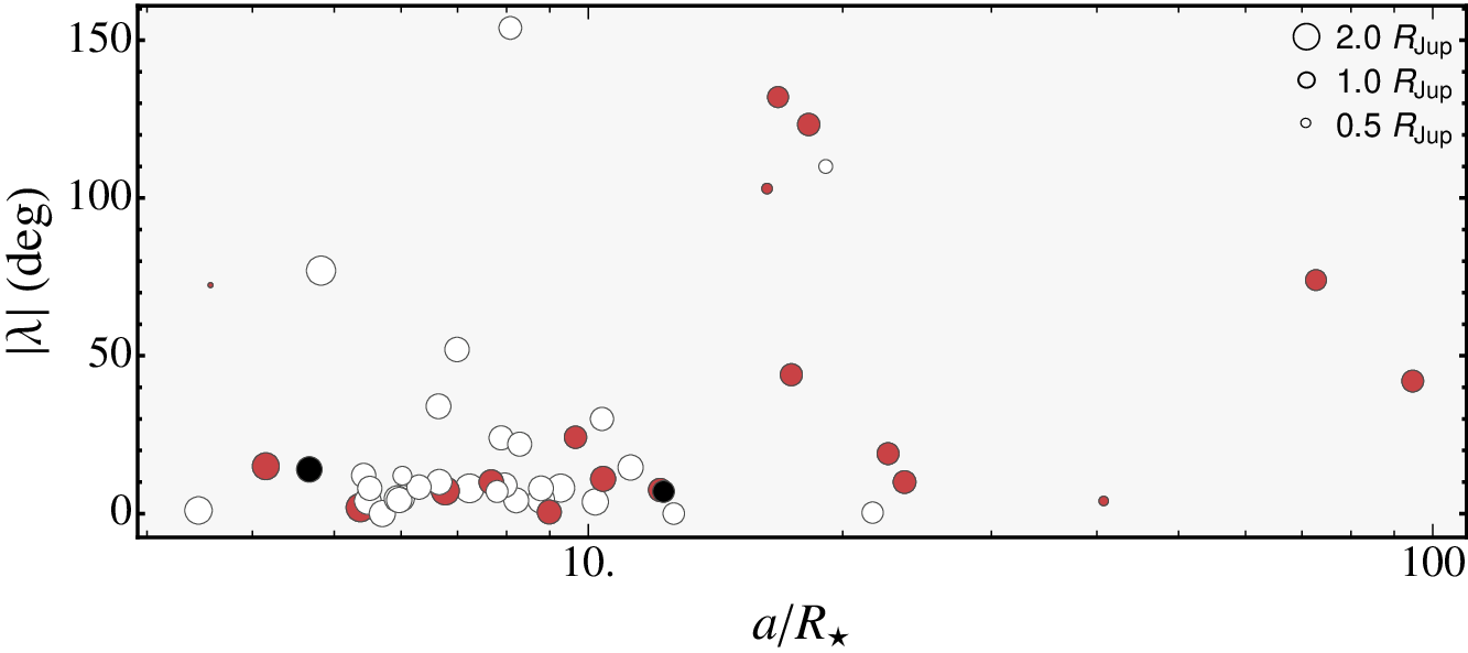
We also plotted in Fig. 13 the projected orbital obliquity of the cool-star systems, i.e., following Anderson et al. (2015), those with K, as a function of orbital distance in units of stellar radii, . However, we do not see an absolute confinement of at any particular orbital-separation range.
According to TEPCat, there are now 12 TEP systems for which we have the measurement of the true obliquity, i.e. the angle, , between the axes of the stellar rotation and the planetary orbit. These values are plotted against the stellar temperature in Fig. 14 that, again, does not highlight any correspondence between the two quantities.
Based on a recent gyrochronology work by Meibom et al. (2015), the rotation period of HAT-P-36, estimated in Sect. 3.3, should correspond to an age of about 1.8 Gyr, which is close to the lower limit reported in Table 8, as derived from our isochrone-fitting analysis. Since the planet is very close to its host, we may speculate about tidal interactions affecting the evolution of the orbit and of the stellar spin. Assuming a modified tidal quality factor , the remaining lifetime of the system – i.e., the time left before the planet plunges into the star – is only 35 Myr (Metzger et al., 2012). Such a rapid orbital decay should be accompanied by a negative transit time variation O-C of about 20 seconds in ten years that would be easy to measure with a space-borne photometer. On the other hand, if we assume , as suggested by Ogilvie & Lin (2007), the orbital decay and alignment timescales are of the order of a few hundred Myr or a few Gyr, respectively. They are shorter than or comparable to the estimated age of the star. In conclusion, in this scenario the present alignment could result from the tidal interaction during the main-sequence lifetime, while the remaining lifetime of the system is at least of a few hundred Myr. In any case, HAT-P-36 is an interesting system to study the orbital and stellar spin evolution, as resulting from the tidal interaction and the magnetic wind braking of the star.

For WASP-11, the relatively large semi-major axis and the small mass of the planet imply, on the other hand, a weak tidal interaction with an angular momentum exchange timescale that is comparable or longer than the age of the star. Therefore, the observed projected alignment of the system is likely to be of primordial origin.
7 Summary and conclusions
In the framework of the GAPS programme, we are observing a sample of TEP systems hosting close-in hot Jupiters, with the HARPS-N spectrograph. The goal is to measure their spin-orbit alignment (by observing the RM effect) and study if this quantity is correlated with other physical properties. Here, we have presented an exhaustive study of the HAT-P-36 and WASP-11/HAT-P10 planetary systems, based on data collected with four telescopes during transit events.
By analysing these new photometric and spectroscopic data, we revise the physical parameters of these two systems, finding that previous determinations agree with our more accurate results, within the uncertainties.
Interestingly, we observed anomalies in three photometric transit light curves of HAT-P-36 that, after appropriate modelling, turned out to be compatible with starspot complexes on the photosphere of the star. The main characteristics of the starspots were estimated and compared with those observed in other TEP systems. The HAT-P-36 starspot activity is confirmed by the analysis of the HARPS-N spectra, which give a stellar activity index of dex, and by study of the whole photometric data set collected by the HATNet survey. The frequency analysis of this time-series data revealed a clear modulation in the light curve caused by starspots, allowing us to get an accurate measurement of the rotational period of the star, days. A similar study, performed for WASP-11/HAT-P-10 on both the WASP and HATNet survey light curves, did not highlight any clear photometric modulation.
The RM effect was partially covered in HAT-P-36 (because of bad weather conditions) and wholly observed in WASP-11/HAT-P-10. Thanks to the high-resolution HARPS-N spectra, the sky projection of the orbital obliquity was successfully measured for both the systems, indicating a good spin-orbit alignment. In particular, for the HAT-P-36 system, we were able to also estimate its real obliquity, obtaining degrees. Our results are thus in agreement with the idea that stars with relatively cool photospheres should have small spin-orbit misalignment angles. However, looking at the entire sample of known TEP systems, for which we have an accurate estimation of , there are several exceptions to this scenario. In this context, the case of HAT-P-18 b (Esposito et al., 2014) is emblematic. The collection of more data is thus mandatory for disentangling the issue and understanding whether orbital obliquity really holds imprints of past migration processes that dramatically affected the evolution of giant planets.
Acknowledgements.
The HARPS-N instrument has been built by the HARPS-N Consortium, a collaboration between the Geneva Observatory (PI Institute), the Harvard-Smithonian Center for Astrophysics, the University of St. Andrews, the University of Edinburgh, the Queen’s University of Belfast, and INAF. Operations at the Calar Alto telescopes are jointly performed by the Max-Planck Institut für Astronomie (MPIA) and the Instituto de Astrofísica de Andalucía (CSIC). The reduced light curves presented in this work will be made available at the CDS (http://cdsweb.u-strasbg.fr/). The GAPS project in Italy acknowledges support from INAF through the “Progetti Premiali” funding scheme of the Italian Ministry of Education, University, and Research. We acknowledge the use of the following internet-based resources: the ESO Digitized Sky Survey; the TEPCat catalog; the SIMBAD data base operated at CDS, Strasbourg, France; and the arXiv scientific paper preprint service operated by Cornell University.References
- Albrecht et al. (2012a) Albrecht, S., Winn, J. N., Butler, R. P., et al. 2012a, ApJ, 744, 189
- Albrecht et al. (2012b) Albrecht, S., Winn, J. N., Johnson, J. A., et al. 2012b, ApJ, 757, 18
- Anderson et al. (2010) Anderson, D. R., Hellier, C., Gillon, M., et al. 2010, ApJ, 709, 159
- Anderson et al. (2015) Anderson, D. R., Triaud, A. H. M. J., Turner, O. D., et al. 2015, ApJ, 800, L9
- Bakos et al. (2009) Bakos, Á G., Pál, A., Torres, G., et al. 2009, ApJ, 696, 1950
- Bakos et al. (2012) Bakos, Á G., Hartman, J. D., Torres, G., et al. 2012, AJ, 144, 19
- Baranne et al. (1996) Baranne, A., Queloz, D., Mayor, M., et al. 1996, A&AS, 119, 373
- Berdyugina (2005) Berdyugina, S. V. 2005, Living Rev. Sol. Phys., 2, 8
- Biazzo et al. (2012) Biazzo, K., D’Orazi, V., Desidera, S., et al. 2012 MNRAS, 427, 2905
- Brothwell et al. (2014) Brothwell, R. D., Watson, C. A., Hébrard, G., et al., 2014, MNRAS, 440, 3392
- Bryan et al. (2012) Bryan, M. L., et al., 2012, ApJ, 750, 84
- Casagrande et al. (2010) Casagrande, L., Ramírez, I., Meléndez, J., Bessell, M., Asplund, M. 2010, A&A 512, A54
- Ciceri et al. (2013) Ciceri, S., Mancini, L., Southworth, J., et al. 2013, A&A, 557, A30
- Claret (2004) Claret, A. 2004, A&A, 424, 919
- Cosentino et al. (2012) Cosentino, R., Lovis, C., Pepe, F., et al. 2012, in Proc. SPIE, 8446, 1V
- Covino et al. (2013) Covino, E., Esposito, M., Barbieri, M., et al. 2013, A&A, 554, A28
- Damasso et al. (2015) Damasso, M., Biazzo, K., Bonomo, A. S., et al. 2015, to appear in A&A, arXiv:1501.01424
- Dawson (2014) Dawson, R. I. 2014, ApJ, 790, 31
- Demarque et al. (2004) Demarque, P., Woo, J.-H., Kim, Y.-C., Yi, S. K. 2004, ApJS, 155, 667
- Desidera et al. (2013) Desidera, S., Sozzetti, A., Bonomo, A. S., et al. 2013, A&A, 554, A29
- Desidera et al. (2014) Desidera, S., Bonomo, A. S., Claudi, R. U., et al. 2014, A&A, 567, L6
- Dotter et al. (2008) Dotter, A., Chaboyer, B., Jevremovic̀, D., et al. 2008, ApJS, 178, 89
- Ehrenreich & Désert (2011) Ehrenreich, D., Désert, J.-M. 2011, A&A, 529, A136
- Esposito et al. (2014) Esposito, M., Covino, E., Mancini, L., et al. 2014, A&A, 564, L13
- Hébrard et al. (2011) Hébrard, G., Ehrenreich, D., Bouchy, F., et al. 2011, A&A, 527, L11
- Hilditch (2001) Hilditch, R. W. 2001, An Introduction to Close Binary Stars, (Cambridge, UK: Cambridge University Press)
- Huitson et al. (2013) Huitson, C. M., Sing, D. K., Pont, F., et al. 2013, MNRAS, 434, 3252
- Knutson et al. (2007) Knutson, H. A., Charbonneau, D., Noyes, R. W. 2007, ApJ, 655, 564
- Knutson et al. (2010) Knutson, H. A., Howard, A. W., Isaacson, H. 2010, ApJ, 720, 1569
- Kovács et al. (2005) Kovács, G., Bakos, G. Á., Noyes, R. W. 2005, MNRAS, 356, 557
- Kuschnig et al. (1997) Kuschnig, R., Weiss, W. W., Gruber, R., Bely, P. Y., Jenkner, H. 1997, A&A, 328, 544
- Lai (2012) Lai, D. 2012, MNRAS, 423, 486
- Lendl et al. (2014) Lendl, M., Triaud, A. H. M. J., Anderson, D. R., et al. 2014, A&A, 568, A81
- Lund et al. (2014) Lund, M. N., Lundkvist, M., Silva Aguirre, V., et al. 2014, A&A, 570, A54
- Maciejewski et al. (2013) Maciejewski, G., Puchalski, D., Saral, G., et al. 2013, IBVS, 6082, 1
- Mamajek & Hillenbrand (2008) Mamajek, E. E., Hillenbrand, L. A. 2008, ApJ, 687, 1264
- Mancini et al. (2013a) Mancini, L., Southworth, J., Ciceri, S., et al. 2013a, A&A, 551, A11
- Mancini et al. (2013b) Mancini, L., Ciceri, S., Chen, G., et al. 2013b, MNRAS, 436, 2
- Mancini et al. (2014b) Mancini, L., Southworth, J., Ciceri, S., et al. 2014b, MNRAS, 443, 2391
- Mayor & Queloz (1995) Mayor, M., Queloz, D. 1995, Nature, 378, 355
- Meibom et al. (2015) Meibom, S., Barnes, S. A., Platais, I., et al. 2015, Nature, 517, 589
- Metzger et al. (2012) Metzger, B. D., Giannios, D., Spiegel, D. S. 2012, MNRAS, 425, 2778
- Mohler-Fischer et al. (2013) Mohler-Fischer, M., Mancini, L., Hartman, J., et al. 2013, A&A, 558, A55
- Mordasini et al. (2014) Mordasini, C., Mollière, P., Dittkrist, K.-M., et al. 2014, to appear in IJA, arXiv:1406.5604
- Noyes et al. (1984) Noyes, R. W., Hartmann, L. W., Baliunas, et al. 1984, ApJ, 279, 763
- Ogilvie & Lin (2007) Ogilvie, G., & Lin, D. 2007, ApJ, 661, 1180
- Pepe et al. (2002) Pepe, F., Mayor, M., Galland, F., et al. 2002, A&A, 388, 632
- Pietrinferni et al. (2004) Pietrinferni, A., Cassisi, S., Salaris, M., Castelli, F. 2004, ApJ, 612, 168
- Rabus et al. (2009) Rabus, M., Alonso, R., Belmonte, J. A., et al. 2009, A&A, 494, 391
- Rogers & Lin (2013) Rogers, T. M., Lin, D. N. C. 2013, ApJ, 769, 10
- Sada et al. (2012) Sada, P. V., Deming, D., Jennings, D. E., et al. 2012, PASP, 124, 212
- Sanchis-Ojeda et al. (2011) Sanchis-Ojeda, R., Winn, J. N., Holman, M. J. 2011, ApJ, 733, 127
- Sanchis-Ojeda et al. (2013) Sanchis-Ojeda, R., Winn, J. N., Marcy, G. W. 2013, ApJ, 775, 54
- Seager & Mallén-Ornelas (2003) Seager, S., Mallén-Ornelas, G. 2003, ApJ, 585, 1038
- Silva (2003) Silva, A. V. R. 2003, ApJ, 585, L147
- Silva-Valio et al. (2010) Silva-Valio, A., Lanza, A. F., Alonso, R., Barge, P. 2010, A&A, 510, A25
- Sing et al. (2011) Sing, D. K., Pont, F., Aigrain, S., et al. 2011, MNRAS, 416, 1443
- Sneden (1973) Sneden, C. 1973, ApJ, 184, 839
- Southworth (2008) Southworth, J. 2008, MNRAS, 386, 1644
- Southworth (2011) Southworth, J. 2011, MNRAS, 417, 2166
- Southworth (2012) Southworth, J. 2012, MNRAS, 426, 1291
- Southworth (2013) Southworth, J. 2013, A&A, 557, 119
- Southworth et al. (2007) Southworth, J., Wheatley, P. J., Sams, G. 2007, MNRAS, 379, L11
- Southworth et al. (2014) Southworth, J., Hinse, T. C., Burgdorf, M., et al., 2014, MNRAS, 444, 776
- Sozzetti et al. (2007) Sozzetti, A., Torres, G., Charbonneau, D., et al. 2007, ApJ, 664, 1190
- Strassmeier (2009) Strassmeier, K. G. 2009, Astron. Astrophys. Rev., 17, 251
- Tregloan-Reed et al. (2013) Tregloan-Reed, J., Southworth, J., Tappert, C. 2013, MNRAS, 428, 3671
- Tregloan-Reed et al. (2015) Tregloan-Reed, J., Southworth, J., Burgdorf, M. 2015, MNRAS in press, arXiv:1503.09184
- Triaud et al. (2010) Triaud, A. H. M. J., Collier Cameron, A., Queloz, D., et al. 2010, A&A, 524, A25
- Valsecchi & Rasio (2014) Valsecchi, F., Rasio, F. A. 2014, ApJ, 786, 102
- VandenBerg et al. (2006) VandenBerg, D. A., Bergbusch, P. A., Dowler, P. D. 2006, ApJS, 162, 375
- Vaniĉek (1971) Vaniĉek, P. 1971, Ap&SS, 12, 10
- Wang et al. (2014) Wang, X., Gu, S., Collier Cameron, A., et al. 2014, AJ, 147, 92
- West et al. (2009) West, R. G., Collier Cameron, A., Hebb, L., et al. 2009, A&A, 502, 395
- Winn et al. (2007) Winn, J. N., Holman, M. J., Henry, G. W., et al. 2007, AJ, 133, 1828
- Winn et al. (2010) Winn, J. N., Fabrycky, D., Albrecht, S., Johnson, J. A. 2010, ApJ, 718, L145
- Xue et al. (2014) Xue, Y., Suto, Y., Taruya, A., et al. 2014, ApJ, 784, 66
Appendix A Supplementary tables
The tables in this Appendix contain the detailed results of the predictions of different sets of stellar evolutionary models for the HAT-P-36 and WASP-11/HAT-P-10 planetary systems. The final values of the physical parameters for each of the two systems (see Tables 8 and 9), are calculated by taking the unweighted mean of the five estimates of the different sets of model predictions (see Sect 5).
| (Claret models) | (Y2 models) | (BaSTI models) | (VRSS models) | (DSEP models) | ||||||
| ( km s-1) | 196.19 | 4.95 | 196.09 | 1.79 | 193.00 | 1.62 | 193.00 | 2.76 | 196.17 | 0.32 |
| () | 1.0503 | 0.0840 | 1.0486 | 0.0287 | 1.0000 | 0.0259 | 1.0000 | 0.0426 | 1.0500 | 0.0045 |
| () | 1.048 | 0.029 | 1.047 | 0.012 | 1.031 | 0.013 | 1.031 | 0.018 | 1.048 | 0.010 |
| (cgs) | 4.4192 | 0.0132 | 4.4190 | 0.0100 | 4.4121 | 0.0092 | 4.4121 | 0.0109 | 4.4192 | 0.0085 |
| () | 1.877 | 0.130 | 1.875 | 0.088 | 1.816 | 0.087 | 1.816 | 0.095 | 1.876 | 0.079 |
| () | 1.313 | 0.038 | 1.312 | 0.020 | 1.291 | 0.021 | 1.291 | 0.025 | 1.313 | 0.018 |
| () | 0.776 | 0.049 | 0.776 | 0.046 | 0.789 | 0.047 | 0.789 | 0.048 | 0.776 | 0.047 |
| 0.0654 | 0.0033 | 0.0654 | 0.0030 | 0.0665 | 0.0030 | 0.0665 | 0.0032 | 0.0654 | 0.0030 | |
| (AU) | 0.024040 | 0.000605 | 0.024028 | 0.000219 | 0.023651 | 0.000198 | 0.023651 | 0.000338 | 0.024038 | 0.000036 |
| Age (Gyr) | ||||||||||
| (Claret models) | (Y2 models) | (BaSTI models) | (VRSS models) | (DSEP models) | ||||||
|---|---|---|---|---|---|---|---|---|---|---|
| ( km s-1) | 129.9 | 3.2 | 127.7 | 2.0 | 127.5 | 1.9 | 127.5 | 2.3 | 128.4 | 2.1 |
| () | 0.846 | 0.063 | 0.804 | 0.039 | 0.800 | 0.036 | 0.800 | 0.043 | 0.818 | 0.038 |
| () | 0.785 | 0.023 | 0.772 | 0.013 | 0.771 | 0.015 | 0.771 | 0.014 | 0.777 | 0.012 |
| (cgs) | 4.576 | 0.016 | 4.569 | 0.016 | 4.568 | 0.015 | 4.568 | 0.018 | 4.571 | 0.018 |
| () | 0.508 | 0.028 | 0.492 | 0.020 | 0.490 | 0.019 | 0.490 | 0.024 | 0.497 | 0.023 |
| () | 1.006 | 0.031 | 0.989 | 0.019 | 0.987 | 0.020 | 0.987 | 0.023 | 0.995 | 0.022 |
| () | 0.467 | 0.028 | 0.475 | 0.025 | 0.476 | 0.026 | 0.476 | 0.027 | 0.472 | 0.026 |
| 0.0531 | 0.0021 | 0.0540 | 0.0016 | 0.0541 | 0.0017 | 0.0541 | 0.0019 | 0.0537 | 0.0019 | |
| (AU) | 0.04447 | 0.00111 | 0.04373 | 0.00069 | 0.04365 | 0.00065 | 0.04365 | 0.00080 | 0.04398 | 0.00070 |
| Age (Gyr) | … | … |