The Structure of the Nucleon: Elastic Electromagnetic Form Factors
Abstract
Precise proton and neutron form factor measurements at Jefferson Lab, using spin observables, have recently made a significant contribution to the unraveling of the internal structure of the nucleon. Accurate experimental measurements of the nucleon form factors are a test-bed for understanding how the nucleon’s static properties and dynamical behavior emerge from QCD, the theory of the strong interactions between quarks. There has been enormous theoretical progress, since the publication of the Jefferson Lab proton form factor ratio data, aiming at reevaluating the picture of the nucleon. We will review the experimental and theoretical developments in this field and discuss the outlook for the future.
pacs
PACS-key13.40.Gp and PACS-key13.85.Dz1 Introduction
One of the fundamental goals of nuclear physics is to understand the structure and behavior of strongly interacting matter in terms of its basic constituents, quarks and gluons. Quantum chromodynamics (QCD) is the theory of the strong interaction, responsible for binding quarks through the exchange of gluons to form hadrons (baryons and mesons). The electromagnetic form factors are among the most basic quantities containing information about the internal structure of the proton and neutron, together known as nucleons. The challenge of understanding the nucleon’s structure and dynamics has occupied a central place in nuclear physics. High energy electron scattering provides one of the most powerful tools to investigate the structure of nucleons.
Early electron scattering experiments with nuclei were motivated by a need to verify predictions of the then current models of the electromagnetic interaction of electrons with nuclei, and in particular with the proton and neutron; Rosenbluth predicted that high energy electrons would be scattered dominantly by the magnetic moment of the proton [1]. Available accelerators in the early fifties had energies smaller than 50 MeV, and provided information on the nuclear radius of elements from Be to Pb. The first clear evidence that the proton has a structure was obtained at the High Energy Physics Laboratory (HEPL) at Stanford in the period form 1953 to 1956, under the leadership of Robert Hofstadter [2]. A proton charge radius of 0.77 fm was extracted by Chambers and Hofstadter [3] from the electron-proton data obtained using the electron beams with energies up to 550 MeV at the HEPL, confirming that the proton has a finite size. In his review paper Hofstadter [4] discussed in detail the extraction of proton charge and magnetization radii between 0.72 and 0.80 fm using different models. Almost sixty years after the work of Hofstadter [4], the question of whether the proton radius is 0.8775 (51) fm, the CODATA [5] value from elastic scattering, or is 0.84087 (39) fm [6], the muonic hydrogen value, which is a difference of seven standard deviations, is being discussed intensely.
A similar change in accepted concepts occurred when the data, which was obtained at the Thomas Jefferson National Accelerator Facility (TJNAF) or Jefferson Lab (JLab) for the proton’s electric to magnetic form factor ratio, from double polarization experiments and completed in 2000 at a four momentum transfer squared, , of up to 5.6 GeV2 [7, 8, 9, 10], differed drastically from the form factor results obtained with the cross sections data using the Rosenbluth separation method [11, 12, 13, 14, 15, 16, 17, 18, 19, 20, 21, 22]. The standard form factor database up to 1990’s had been entirely defined by cross section measurements, and suggested that, for GeV2, the ratio , where is the magnetic moment of the proton. The double polarization experiments at JLab demonstrated that decreased approximately linearly with for GeV2, dropping to a value of 0.35 at = 5.6 GeV2 which was the highest investigated at that time.
In the last several years, the field of nucleon structure has been investigated extensively. Two recent experiments at JLab have increased the range of the and data. These data have triggered much activity in the determination of the flavor separated form factors of the dressed up- and down quarks in the nucleon. Experiments at Mainz, JLab and MIT-Bates have resulted in a much better coverage of the low range for , contributing to the intensive discussion of a possible disagreement between electron elastic scattering and muonic hydrogen data used to determine the proton radius. Several experiments have measured the e+/e- cross section ratio for the proton with a level of precision that tests recent calculations which included two photon exchange contributions to the cross sections. A direct measurement of the two photon contribution to the double polarization observables was undertaken at JLab. The results confirm the expectation that two photon exchange affects the proton form factor ratio at less than the percent level. Combining these various experiments and theoretical calculations, the possible role of two photon exchange in bridging the gap in the extraction of the proton form factors from cross section and double polarization observables can be investigated.
1.1 History of Elastic Electron Scattering on the Nucleon
Elastic electron proton scattering has evolved since the history making series of experiments with electron beams of the HEPL at Stanford in 1950s. Under the leadership of R. Hofstadter, a series of crucial results were obtained from cross section measurements [23]. Several fundamental pieces of information were established following these experiments, including the approximate decrease of the cross section with , establishing the approximate shape of the charge distribution, and a first value for the proton radius. Theoretical work evolved in parallel with these experimental “firsts”, leading to the description of the elastic electron scattering in terms of the lowest order process, the exchange of a single virtual photon with negative invariant mass squared; this lowest order contribution, also called the Born term, was expected to be dominant because of the smallness of the electromagnetic coupling constant . Fundamental expressions for the hadronic current and the definition of two invariant form factors, and , later named the Dirac and Pauli form factors, of the Born term, were issues of this period. In 1957 Yennie, Levy and Ravenhall [24] derived an expression for the cross section in terms of these two form factors, and , following Rosenbluth’s work [1], as given in Eq. 3.
The possibility of measuring either the polarization transferred to the recoil proton, or the asymmetry if the target proton or neutron is polarized, with longitudinally polarized electrons, was discussed in a paper by Akhiezer et al. [25] in 1957. It was to be more than 30 years before such experiments, which require a polarized electron beam, could be performed with good accuracy. Further papers on double polarization experiments followed, including Scofield [26], Akhiezer and Rekalo [27, 28], Dombey [29], and Arnold, Carlson and Gross [30].
The construction of the Continuous Electron Beam Accelerator Facility (CEBAF) at JLab, in Virginia, led to an intensive program of nucleon form factor measurements, first for the proton and then for the neutron, and a significant breakthrough in our understanding of the proton structure. In the Born approximation the transferred polarization has only two non-zero components, both in the reaction plane defined by the beam and scattered electron, one along the recoil proton momentum, and the other perpendicular to it. For the proton, polarization transfer has been used most often at JLab [7, 8, 9, 10]; it requires a re-scattering of the proton to measure its polarization. For the neutron, target asymmetry has now been used successfully [31, 32, 33] for the determination of the ratio; this requires a polarized target of either or , which limits the maximum electron current that can be tolerated without significant depolarization of the target.
Among the earliest electron-proton scattering polarization experiments is a search in 1963 at the Orsay linear accelerator, for a one-photon/two-photon interference effect with an un-polarized electron beam and an un-polarized target. They searched for normal and transverse polarization components. The normal polarization component was found to be 0.040 0.027; the transverse polarization component was 0.000 0.028 at of 0.61 GeV2[34].
A similar single-spin experiment in 1970 with an un-polarized 15–18 GeV electron beam at the Stanford linear accelerator, and a polarized proton target with polarization perpendicular to the reaction plane to characterize the interference of the two-photon exchange with the single photon exchange (Born) process, produced asymmetries of order 1 to 2 % in the range of 0.38 to 0.98 GeV2 [35].
On the neutron side, the pioneering experiment of Madey et al. performed the first recoil polarization measurement of at a -value of 0.255 GeV2 in 1994 [36] at the MIT BATES Linear Accelerator; and the first double polarization measurement of the proton form factor ratio, , was also carried out at the same lab in 1994-1995 by measuring the two polarization transfer components Pℓ and Pt, at -values of 0.38 to 0.50 GeV2 [37, 38, 39].
Also the mid nineties saw a number of double polarization experiments at Nationaal Instituut voor Kernfysica en Hoge Energie Fysica (NIKHEF) [40] and Mainz Microtron (MAMI) [41, 42] to determine the neutron electric form factor up to 1 GeV2. All experiments used polarized electron beams and a polarized target, either or .
In this review, we will focus on the space-like nucleon form factors, as in the past 15 years they have been studied more extensively both experimentally and theoretically, compared to the time-like nucleon form factors [43]. Also the strangeness form factors are not discussed in this review; see Ref. [44] for a review of the field of parity violating electron scattering and strangeness form factors.
This review is organized as follows. Section 2 describes the formalism of elastic electron scattering on the nucleon. In subsection 2.1, the use of elastic differential cross section data to extract the two electromagnetic form factors of proton and neutron by the Rosenbluth, or longitudinal and transverse (LT)-separation technique is reviewed. Subsection 2.2 discusses how the form factors are measured in the double polarization experiments. The two photon exchange formalism is explained in subsection 2.3.
Section 3 is devoted to discuss the experimental status. Subsection 3.1 describes the experiments which extracted the electric and magnetic form factors for the proton and the neutron from measurements of cross sections. Subsection 3.2 reviews the status of the double polarization experiments and discuss the results for the proton and the neutron, obtained from the recoil polarization method and beam-target asymmetry measurements. The role of two photon exchange contributions in the elastic reaction in resolving the discrepancy between the proton’s electric form factor extracted by recoil polarization versus the Rosenbluth separation technique are discussed in subsection 3.3. Subsection 3.4 reviews the present status of the proton charge radius. Subsection 3.5 discusses the present status of flavor separation of nucleon form factors.
Section 4 deals with the theoretical interpretations of the electromagnetic nucleon form factors. Subsection 4.1 reviews the models of the nucleon form factors. These models include conformal fits to the form factors, vector meson dominance, dispersion analysis, constituent quark models, pion cloud models, transverse densities, and correspondences with higher dimensional theories. Subsection 4.2 describes the Dyson-Schwinger equations and diquark models. Subsection 4.3 discusses links between deep-inelastic scattering and nucleon form factors which includes perturbative QCD inspired models and generalized parton distribution (GPD) models. Subsection 4.4 describes lattice QCD calculations of nucleon form factors.
Section 5 summarizes the current issues and challenges in the area of electromagnetic form factors. This section closes with a discussion of future experiments at Jefferson Lab which will measure the proton and neutron form factors to =10 GeV2 or greater.
2 Formalism of Elastic Electron Nucleon Scattering
The lowest order approximation for electron nucleon scattering is the single virtual photon exchange process, or Born term. The Born approximation is expected to provide a good lowest order description of elastic scattering (with ) because of the weak electro-magnetic coupling of the photon with the charge and the magnetic moment of the nucleon. The amplitude for the process is the product of the four-component leptonic and hadronic currents, and , and can be written as:
| (1) | |||||
where are the the four-momenta of the incident and scattered, electron and proton, respectively, contains all information of the nucleon structure, and is the metric tensor. To insure relativistic invariance and the correct parity property of the amplitude , can only contain p, p’ and , besides numbers, masses and , defined as, , is the negative of the square of the invariant mass, , of the virtual photon exchanged in the one-photon approximation of scattering.
The most general form for the hadronic current for the spin -nucleon, satisfying relativistic invariance
and current conservation, and including an internal structure is:
| (2) |
where is the nucleon mass; is the anomalous magnetic moment, in units of the nuclear magneton, . The Dirac and Pauli form factors, and are the only structure functions allowed in the Born term by relativistic invariance. As is now the most frequently used notation, will be written as and , respectively. In the static limit, , , and and , for the proton and neutron, respectively.
2.1 Cross Section Experiments
The Lab frame differential cross section for detection of the electron in elastic or scattering is then:
| (3) | |||||
with . The Mott cross section is:
| (4) |
The incident electron (beam) and scattered electron energies are labeled and , respectively. The fraction in Eq. (3) is the recoil correction to the Mott cross section.
Experimental cross section data are most easily analyzed in terms of another set of form factors, the Sachs form factors and [45, 46]. The relations between and and and for proton and neutron are:
| (5) |
The scattering cross section Eq. (3) can then be written in a simpler form, without an interference term, leading to a separation method for and known as Rosenbluth (or Longitudinal-Transverse) technique, as will be seen below. Now the cross section is:
| (6) |
where is the polarization of the virtual photon defined as:
| (7) |
The Rosenbluth separation technique takes advantage of the linear dependence in , in the reduced cross section , based on Eq. (6), as follows:
| (8) | |||||
showing that is expected to have a linear dependence on , with the slope proportional to and the intercept equal to .
2.2 Double Polarization Experiments
In 1968 and 1974 Akhiezer and Rekalo [27, 28] discussed the interest of measuring an interference term of the form by observing the transverse component of the recoiling proton polarization in at large , to obtain in the presence of a dominating . In a review paper Dombey [29] emphasized the virtues of measurements with a polarized lepton beam on a polarized target to obtain polarization observables. Also later in 1981 Arnold, Carlson and Gross [30] discussed in detail, that the best way to measure the neutron and proton form factors would be to use the and reactions, respectively.
Indeed, both the recoil polarization and target asymmetry measurement methods have been used successfully to measure the proton and neutron form factors to high four momentum transfer, , at JLab. The same methods have been used also at MIT-Bates, MAMI, and NIKHEF, to make precise proton and neutron form factor measurements at lower . Both methods are discussed below, with benefits and drawbacks of using polarized target and/or focal plane polarimeter.
2.2.1 Recoil Polarization Method
With a longitudinally polarized electron beam and an unpolarized target, the polarization of the incoming electron is transferred to the nucleon (proton or neutron) via exchange of a single virtual photon as shown in Fig. 1. For elastic scattering, in the single photon exchange approximation, with a longitudinally polarized electron beam, the only non-zero polarization transfer components are the longitudinal and transverse, and . The normal polarization transfer component, , is zero. For single photon exchange, the transferred polarization components can be written in terms of the Sachs form factors as:
| (9) |
where are the beam helicity states, is the magnitude of polarization, and is the electron scattering angle.

The ratio of to is then directly obtained from the ratio of the two polarization components and as:
| (10) |
The double-polarization approach to obtain the ratio at the large momentum transfer by measuring two polarization components simultaneously was first proposed at JLab in 1989 [47]; it is based on a combination of spin precession in a magnetic spectrometer and using a proton polarimeter. The major advantage of the method, compared to cross section measurements, is that in the Born approximation, for each , a single measurement of the azimuthal angular distribution of the proton scattered in a secondary target gives both the longitudinal, , and transverse, , polarization. Thus the ratio of electric to magnetic form factors of the proton is obtained directly from a simultaneous measurement of the two recoil polarization components. The knowledge of the beam polarization and of the analyzing power of the polarimeter is not needed to extract the ratio, , strongly decreasing the systematic uncertainties. The kinematic factors in Eq. (10) are typically known to a precision far greater than the statistical precision of the recoil polarization components.
2.2.2 Asymmetry with Polarized Targets
It was discussed by Dombey [29] in a review paper in 1969 that the nucleon form factors can be extracted from the scattering of longitudinally polarized electrons off a polarized nucleon target. In the one photon exchange approximation, the elastic electron nucleon scattering cross section can be written as a sum of two parts: , which corresponds to the unpolarized elastic differential cross section given by Eq. (6), and a polarized part, , which is non-zero only if the electron beam is longitudinal polarized [48, 49];
| (11) |
The polarized part of the cross section, , with two terms related to the directions of the target polarization, , is given by [48, 49]:
| (12) | |||||
where and are the polar and azimuthal laboratory angles of the target polarization vector with in the direction and normal to the electron scattering plane, as shown in Figure 2.

The physical asymmetry is then defined as
| (13) |
where and are the cross sections for the two beam helicity states.
For a longitudinally polarized beam and polarized target, the measured asymmetry, , is related to the physical asymmetry, , by
| (14) |
where and are electron beam and target polarization, respectively, and can be obtained using Eqs. (6) and (12),
| (15) | |||||
From Eq. (15), it is apparent that to extract , the target polarization in the laboratory frame must be perpendicular with respect to the momentum transfer vector and within the reaction plane, with and or . For these conditions, the physical asymmetry in Eq. (15) simplifies to:
| (16) |
As is quite small, is approximately proportional to . In practice, the second term in Eq. (15) is not strictly zero due to the finite acceptance of the detectors, but these effects are small and depend on kinematics only in first order and can be corrected for, so the ratio is not affected directly. One can also note that .
The discussion above is only applicable to a free electron-nucleon scattering. For a quasi-elastic electron scattering from a nuclear targets, like 2H or 3He, corrections are required for several nuclear effects.
2.3 Two-photon exchange
In the one-photon exchange process, the form factors depend only on but not on other kinematic variables. A deviation in the form factors from constant when varying the kinematics (i.e. and the scattered electron angle, keeping constant) would indicate the presence of a mechanism beyond the Born approximation.
In the general case, elastic scattering can be described by three complex amplitudes [50, 51, 52]: , , and , the first two chosen as generalizations of the Sachs electric and magnetic form factors, and , and the last one, , vanishing in case of Born approximation. The reduced cross section, can be written as:
| (17) | |||||
where
| (18) | |||||
| (19) |
and
| (20) |
The polarization transfer components can be written as:
| (21) |
| (22) |
| (23) |
While the Sachs form factors depend only on , in the general case the amplitudes depend also on . The reduced cross section and the polarization transfer components, and are sensitive only to the real part of the two-photon amplitudes. The normal polarization transfer component, , is sensitive to the imaginary parts of the two-photon amplitudes. In the Born approximation, only the first term remains from , and in Eqs. (17), (22) and (23) while is zero.
3 Experimental Status
The structure of the nucleons has been investigated experimentally with rigor over last 70 years using elastic electron scattering. The two Sachs form factors, and , required to describe the nucleon charge- and magnetization distribution have been traditionally obtained by cross section measurements. In the static limit, the proton, , and neutron, , magnetic form factors are equal to the proton, , and neutron, , magnetic moments while the proton, , and neutron, , electric form factors are equal to unity and zero, respectively. The earliest experiments at low found:
| (24) |
The dependence of these form factors can be approximately characterized by a dipole form factor:
| (25) |
The data for have shown good consistency between different experiments up to 30 GeV2, however, the determination of at greater than 2 GeV2 has suffered from large error bars. The neutron electric form factor, , is small and difficult to extract from cross section experiments. New experimental methods using spin observables were needed which pushed the development of polarized targets and new accelerators with high duty factor and polarized electron beams.
The recent generation of electron accelerators with high polarization and high current electron beams, at MIT-Bates, MAMI and JLab, have made it possible to investigate the internal structure of the nucleon with precision. In particular, the new series of experiments that measured spin observables, like beam-target asymmetry and recoil polarization, have allowed experiments to obtain the proton and neutron electromagnetic form factors accurately to large . In this section we describe the proton and neutron form factors obtained from cross sections and double polarization experiments.
3.1 Cross Section Experiments
The electric and magnetic form factors of the nucleon can be extracted from measurements of cross sections at a constant and different beam energies using Eq. (8). This is known as the Rosenbluth separation technique. The strict linearity of the reduced cross section is based on the dominance of one-photon exchange in the elastic electron-nucleon scattering reaction. In principle, only two points are needed to determine the slope, , and intercept, , from Eq. (8). Usually experiments have measured more than two points for a given . From a practical experimental viewpoint, more points allow better understanding and checks of systematic errors. From a theoretical viewpoint, the linearity of the dependence of the reduced cross section can be investigated with more points. One clear sign of a two-photon exchange contribution to the cross section would be a non-linearity in the -dependence of the reduced cross section. Unfortunately, the two-photon exchange contribution can have a linear -dependence which cannot be experimentally separated out in the cross section measurement and must be calculated theoretically. The form factor data presented in the following sections were not corrected for hard two-photon exchange contributions when they were extracted from the elastic scattering measurements.
3.1.1 Proton Form Factors
Extraction of the proton form factors from the cross section data is complicated by the strong dependence of the Mott cross section on the scattering angle. In addition, as can be seen in Eq. (8), the relative contribution of the two form factors to the reduced cross section changes with . This difficulty in measuring both form factors within the same experiment with small errors bars was a problem from the first experiments using the Rosenbluth separation technique. Ref. [11] contains a tabulation of measurements of and from the early 1960’s which are plotted as open triangles in Figs. 3 and 4. From Ref. [11], we have selected to plot only data which have relative error bars of less than 10%. One can see that is measured with this precision only to GeV2 while the data points are plotted only above GeV2.
Throughout the 1960’s, experiments increased their precision. Measurements were done at the Stanford Mark III accelerator of cross sections to 2% statistical precision at between 0.18 to 0.8 GeV2 [12]. Their and values are plotted as multiplication sign symbol in Figs. 3 and 4. In 1971, results on and were published which combined cross section measurements at the Cambridge Electron Accelerator with previous cross section measurements to cover a range of between 0.13 to 1.75 GeV2. The results are plotted in Figs. 3 and 4 as open circles [13]. There is good agreement with the and of Ref. [12] in the region of overlap, while for GeV2 starts to drop-off below unity. In 1970, a SLAC experiment measured and at between 1 to 3.8 GeV2 and found , which is opposite to the trend of Ref. [13]. These data are plotted as filled diamonds in Figs. 3 and 4. In this same time period, and measurements were done at Bonn [15] for between 0.34 to 1.94 GeV2 and at DESY [16] for between 0.67 to 3.0 GeV2. The data from Ref. [15] and [16] are plotted in Figs. 3 and 4 as filled square and crossed diamond, respectively. Both of these data sets agree with the downward trend in for GeV2 seen in Ref.[13], which disagrees with the rise in observed in Ref. [14].
In the 1970’s, a series of experiments at Mainz sought to measure the and form factors at below 0.1 GeV2 with greater precision. The first [17] measured cross sections at between 0.014 to 0.12 GeV2. The second [18] did measurements up to of 0.055 GeV2 with an emphasis on extracting the charge radius of the proton. The and form factors of Ref. [17] and [18] are plotted as crossed square and open square in Figs. 3 and 4. These experiments demonstrate the precision that can be obtained in the measurement of at extremely low . In Sec. 3.4, results from these experiments for the proton charge radius are shown in Fig. 16.
In the late 1960’s and early 1970’s, experiments at SLAC [53] pushed the limits of the cross section measurements to = 25 GeV2. In the 1990’s, an experiment [54] at SLAC measured the cross section at forward angles for from 3 to 30 GeV2 with improved statistical precision. Both experiments extracted under the assumption that / = 1. The data from Ref. [53] (open squares) and [54] (open stars) are plotted in Fig. 4. The data are consistent with each other and show a drop-off in / above GeV2.


In the 1990’s, at SLAC, two experiments were done which extended the precision and upper range of for measurement of by the Rosenbluth separation technique. Ref. [19] measured at of 1.0, 2.0 and 3.0 GeV2. Ref. [20] measured at between 1.75 and 9 GeV2 and this experiment pushed the measurement of to the maximum that has been done at this time. In Figs. 3 and 4, the data of Ref.[19] and [20] are plotted as filled stars and open diamonds, respectively. The data of both experiments agree with each other and previous experiments, while the are very different at = 3 GeV2. The of Ref. [20] agrees well with the early measurements of Ref. [13] at = 1.75 GeV2 and have a flat dependence with a slight rise for GeV2. A global reanalysis of cross section experiments was done by Ref. [57] in 2003. This reanalysis found that the cross section measurements from different experiments were consistent with each other in extraction of both and , though it excluded the small angle data of Ref. [19] from the global analysis.
The data measured by the recoil polarization method will be discussed in the upcoming Sec. 3.2, but the effect on the extraction of will be briefly discussed here. In 2002, an extraction of was done from the cross section data of the previous experiments using the constraint that
which originates from a fit to from the recoil polarization experiments [56]. The fit to the extracted is shown in Fig. 4 as a dashed line and the fit is a few percent larger than from the standard Rosenbluth method. Also shown in Fig. 4 as a solid line is a fit by Ref. [55] to the extracted by Ref. [56] with additional low values from Ref. [58]. Since the time of these fits, the effects of two-photon exchange on the extraction of and have been calculated by theorists and this topic will be discussed in Sec. 3.3.
Taking advantage of the high duty factor of modern accelerators, cross-sections can be measured to high precision over a range of in a relatively short time period. This was recently done with spectacular precision by an experiment at MAMI. Cross sections were measured at 1422 kinematic settings covering a range from 0.004 to 1.0 GeV2 with average point-to-point systematic error of 0.37% [59]. Data were taken with the three separate spectrometers of MAMI at 6 different beam energies. With this large data set, the authors extracted and by fits to their cross section data rather than the traditional Rosenbluth separation technique. The group has published a long paper [60] on the same data set and included other world data in their fits. The sensitivity to different functional forms for the fits was investigated by using many different spline and polynomial forms. The fits also included 31 normalization parameters for possible systematic effects with cross sections measured with the different spectrometers and in different run periods. The fits which had a reduced had a maximum difference in their cross sections of 0.7%.
At JLab, and were measured using the Rosenbluth separation method at between 0.4 to 5.5 GeV2 as part of an experiment to measure inelastic cross sections on a range of nuclei [21]. The results are plotted in Figs. 3 and 4 as asterisk and agree with previous measurements.
Instead of detecting the elastically scattered electron, , an experiment which detected the elastically scattered proton to identify elastic reactions, , was run at JLab in 2002 [22]. The same experimental approach of extracting the form factors by measuring elastic cross sections at fixed and different by varying the beam energy was used. The experimental method takes advantage of the fact that the proton momentum is constant for all at a fixed . In addition for , the detected proton rate and the radiation corrections have a smaller dependence on compared to experiments. All this combines to reduce the dependent systematic error compared to experiments. The form factors were measured at = 2.64, 3.10 and 4.60 GeV2. In Fig. 3 and 4, the measurements of and from the reaction are plotted. The agreement between the form factors extracted by the different experiments is excellent. Experiments which detect either the scattered electrons or the scattered protons have different systematics, so the agreement between the two techniques indicates that the experimental systematic errors are understood.
With the success of the first JLab experiment, a subsequent experiment, E05-017, was run at JLab in Hall C in 2007 [61]. The experiment measured cross-sections at a total of 102 kinematic settings covering a wide range from 0.4 to 5.76 GeV2 with at least three points per . The emphasis was to measure at each as wide an range as possible. Fig. 5 plots the versus for all kinematic points of E05-017. To obtain multiple at the each , 17 different beam energies were needed for the experiment. This number of beam energies in a relatively short time period demonstrate the amazing capabilities in the operation of the Continuous Electron Beam Accelerator at JLab. At = 1 GeV2, thirteen points were measured ranging from = 0.05 to 0.98, with eight of the points above = 0.8. Similarly for = 2.3 GeV2, ten points were measured ranging from = 0.07 to 0.92, with five of the points above = 0.7. The wide range of at a fixed allows a check of the non-linearity in the dependence of the cross-section which would be a sign of two-photon exchange contributions effecting the cross-sections. The effects from two-photon exchange contributions could have a dramatic dependence near = 1.

3.1.2 Neutron Form Factors
The neutron has zero charge and therefore has to be zero at . The slope of at is related to the mean-square radius of the neutron (see Eq. (38) for the proton). Also, the mean-square radius of the neutron, , can be expressed in terms of the neutron-electron scattering length. The neutron-electron scattering length, , can be determined from total transmission cross sections for epithermal and thermal neutrons scattering on the atomic electrons in noble gas targets [62] and lead and bismuth targets [63, 64, 65]. Using results from the total transmission experiments, the Particle Data Group published a recommended value of or [66].
With no free neutron target, cross section experiments have to make measurements on a deuteron target to extract the neutron form factors. Experiments have measured cross sections for quasi-elastic single arm and coincidence reactions. Primarily, the quasi-elastic reaction is a measurement of with limited sensitivity to , since is near zero and much smaller than the proton contribution to the cross section. Single arm quasi-elastic scattering by Ref. [16, 67, 68] can be used to extract but this requires theoretical knowledge of the large final state interactions at low , which leads to a sizable theoretical uncertainty. Coincidence cross section measurements in the reaction were done by [69, 70]. Detection of the neutron in coincidence reduces the theoretical uncertainty and the proton contribution in the extraction, but the uncertainty on the knowledge of the neutron detection efficiency becomes important. In the 1990’s, was measured at MIT-Bates at of 0.11, 0.18 and 0.26 GeV2 using the reaction and the data are plotted in Fig. 6 as open squares. This experiment measured the neutron detection efficiency using the reaction.

Extracting from the ratio of cross sections of the quasi-elastic to reactions is the least sensitive method to uncertainties in the calculation of the deuteron wave function, final state interactions and meson exchange contributions. In the early 1970’s, at DESY, pioneering experiments measuring the ratio of quasi-free cross sections for the to reactions were performed by Ref. [16] and [80]. These experiments extracted at = 0.4, 0.57, 0.78, 1.0 and 1.5 GeV2 and the data are plotted in Fig. 6 as squares with cross.
In 1995, at Bonn, the ratio of quasi-elastic to cross sections was used to extract . was measured at of 0.13, 0.25, 0.42 and 0.61 GeV2 [74] and is plotted in Fig. 6 with empty diamond. The neutron detection efficiency was measured in situ using the reaction. The photons were produced by bremsstrahlung in the hydrogen target.
A series of measurements of the ratio of to cross sections were made in which the neutron detector efficiency was measured by taking the neutron detector to Paul Scherrer Institute (PSI) and using the neutron beam line. A LED system was used to monitor gain and baseline shifts at PSI and during the experiments. The first experiment was done at NIKHEF and was measured at of 0.61 and 0.70 GeV2 [75]. The next experiment was done at MAMI and measurements of were done at of 0.24, 0.50, 0.65 and 0.78 GeV2 [76]. The results from these two experiments are plotted as an asterisk in Fig. 6. These were followed by more measurements of at MAMI which extend the range. The latter experiment was done at values of 0.071, 0.125, 0.36 and 0.89 GeV2 with statistical errors at the 1.5% level and are plotted in Fig. 6 as filled diamonds. Efficiency measurements at PSI were done before and after each experiment and the measurements were consistent. Within this series of experiments, the at matching are in excellent agreement, but are smaller than measured at Bonn [74] and MIT-Bates [73]. Ref. [81] suggested that the Bonn experiment had miscalculated their neutron efficiency, because a contribution from pion electroproduction was not taken into account when determining the neutron efficiency which led to an overestimate of . In their reply [82], Bruins et al responded that in the peaking approximation the contribution from pion electroproduction to their kinematics is negligible. In calculating the contribution from electroproduction, each paper uses a different data set to extrapolate to the measured kinematic region, so, as stated in Ref. [82], the only way to conclusively settle the disagreement is to measure pion electroproduction and photoproduction in the kinematics of the experiment.
At the present time, the highest measurement of was done at SLAC in the early 1980’s by measuring quasi-free cross sections [71]. This experiment measured from of 2.5 to 10 GeV2. Another SLAC experiment [79] measured from of 1.0 to 1.75 GeV2. In the 1990’s, at SLAC, a Rosenbluth separation experiment was done for the quasi-free reaction at = 1.75, 2.5, 3.25 and 4.0 GeV2 and both and were extracted [72]. The values were consistent with zero with large error bars. All experiments have consistent values in the region of overlapping kinematics and their values are plotted in Fig. 6.
The experiment at JLab in Hall B using CLAS measured in fine bins from between 1.0 to 4.8 GeV2 [78]. The data are plotted as open triangles in Fig. 6). A unique feature of this experiment was a dual cell design with liquid hydrogen and deuterium cells separated by 4.7 cm. This allowed measurement of the neutron detection efficiency by the reaction to be done simultaneously with cross section measurements. The Hall B data overlaps nicely with the SLAC measurements. Though at near 4.8 GeV2, the Hall B data set suggest a less rapid fall-off, then measured in the SLAC high data.
Experiments have used elastic cross sections to determine the neutron form factors. The scattering by an electron from the spin 1 deuteron requires 3 form factors in the hadronic current operator, for the charge, quadrupole and magnetic distributions, , and , respectively. In the original impulse approximation form of the cross section developed by Gourdin [83], the elastic cross section is:
| (26) |
where
| (27) |
with . The charge, quadrupole and magnetic form factors can be written in terms of the isoscalar electric and magnetic form factors as follows:
| (28) |
where the coefficients , , and are Fourier transforms of specific combinations of the S- and D-state deuteron wave functions, and [83]. The isoscalar () and isovector () magnetic () and electric () form factors are defined as :
| (29) |
Theoretical knowledge of the deuteron wave function is needed to extract the form factors which is a major systematic uncertainty. Both the magnetic and electric form factors can be extracted from the elastic cross sections, though the range is limited by the theoretical uncertainties. In the 1960’s, elastic cross section measurements were done which determined and for GeV2 [84, 85].
The 1971 DESY experiment of Galster et al. [86] measured elastic cross sections for forward scattered electrons for up to 0.6 GeV2. At these kinematics, the cross section in Eq. (26) is dominated by the term and contributes less than 5% to the term. The data was fitted using different deuteron wave functions and by using
| (30) |
with different parametrization of . The lowest for a fit was obtained using the Feshbach-Lomon [87] deuteron wave function and the following fitting function:
| (31) |
This fit is plotted in Fig. 7 as a dotted line.

The most recent experiment to measure the elastic cross section to determine is that of Platchkov et al. [88]. These data extend to of 0.7 GeV2, with significantly smaller statistical uncertainties than all previous experiments. The form factor is very sensitive to the deuteron wave function, and therefore to the interaction. Furthermore, the shape of cannot be explained by the impulse approximation alone. Corrections for meson exchange currents (MEC) and a small contribution from relativistic effects were found to significantly improve the agreement between calculations and the measured shape of . When fitting the data, a modified form of the Galster fit,
| (32) |
was used. Several potentials which including meson exchange currents as well as relativistic corrections were used to calculate the deuteron wave function. In Fig. 7, the fits of extracted from fitting and in Eq. (32) to the measured are plotted when using the Nijmegen (black solid line) or a Reid soft core (red dashed) potential to calculate the deuteron wave function. Both fits to had similar and the spread between the line gives a sense of the theoretical uncertainty in extracting from the elastic cross section. In 2001, an extraction of was performed using the entire elastic cross section and polarization data [89] and the results are plotted in Fig. 7 as diamonds with the error bars showing the theoretical uncertainty. These data show the limit of using the elastic reaction to determine and the need to use the quasi-elastic polarization observables to extract / which will be discussed in Sec. 3.2.2.
3.2 Double Polarization Experiments
Both the recoil polarization method, and the asymmetry measurement using polarized target, have been used to measure the proton and the neutron form factors. Here we first describe the proton form factor results; the neutron form factor results will be discussed in the next subsection.
3.2.1 Proton Form Factors
The earliest polarization experiments, measuring the polarization of the recoil proton [34], or measuring the asymmetry using a polarized proton target [35] with unpolarized electron beams, were done to search for two photon effects.
The first experiment with polarized electron beam and polarized target was done at the Stanford Linear Accelerator Center (SLAC) in 1970’s [90]. This experiment measured the beam-target asymmetry at = 0.765 GeV2. The experiment showed that the results and the theoretical values were in good agreement if the signs of and are the same.
The recoil polarization method was used for the first time in an experiment at the MIT-Bates laboratory to measure the proton form factor ratio . This experiment determined for a free proton [37, 38], as well as for a bound proton in a deuterium target [39], at -values of 0.38 and 0.5 GeV2. The success of this experiment highlighted the fact that the recoil polarization transfer technique would be of great interest for future measurements of and at higher values, for both the proton and the neutron.
Next, using the same method of measuring the recoil polarization in reaction, the ratio was measured at MAMI at -values of 0.373, 0.401 and 0.441 Gev2 [91]. The ratio results were found to be in agreement with those of Milbrath et al. [37, 38] as well as Rosenbluth measurements.
In the late 1990’s and 2000’s measurements using the recoil polarization method were made at JLab in Hall A and Hall C [92, 93, 94, 95, 96] at low values, as calibration measurements for other polarization experiments. Two new high precision ratio measurements at low were made in Hall A at JLab; the first in 2006 measured the ratio in the range of from 0.2 to 0.5 GeV2 [97], the second in 2008 measured it at of 0.3 to 0.7 GeV2 [98].
The proton form factor ratio has also been obtained by measuring the beam-target asymmetry in the reaction at a of 1.51 GeV2 in a Hall C experiment at JLab in elastic scattering [99]. This is the highest at which the ratio has been obtained from a beam-target asymmetry measurement. The same method was used by the BLAST group at MIT-Bates [100]; this experiment measured the ratio at values of 0.2 to 0.6 GeV2 with high precision.

Figure 8 shows all the low data obtained from recoil polarization experiments [37, 7, 8, 91, 92, 93, 94, 95, 96, 97, 98] and beam-target asymmetry measurements [99, 100] obtained at MIT-Bates, MAMI, and JLab. As can be seen from figure 8, data from different experiments are in general agreement. The slow decrease of the data starts at 0.5 GeV2 and continues to 1.7 GeV2.
A real break-through was made towards the understanding of the internal structure of the proton, when two JLab Hall A and one Hall C experiments obtained the elastic electromagnetic form factor ratio of the proton, at ’s larger than 1 GeV2, from the measured recoil proton polarization components and , using the recoil polarization method. The first of these experiments measured the proton form factor ratios for from 0.5 to 3.5 GeV2 in 1998 [7, 8], the second from 4.0, 4.8 and 5.6 GeV2 in 2000 [9, 10] and the third in 2007-8 up to 8.4 GeV2 [101].
In the first JLab experiment GEp(1), elastic events were selected by detecting the scattered electrons and the recoiling protons in coincidence, using the two identical high-resolution spectrometers (HRS) of Hall A [102]. One of the HRS was equipped with a focal plane polarimeter (FPP) to detect the polarization of the recoil protons. The FPP consisted of two front detectors to track incident protons, followed by a graphite analyzer and two rear detectors to track scattered particles. The polarization of the recoiling proton was obtained from the asymmetry of the azimuthal distribution of the proton after re-scattering in the graphite analyzer of the polarimeter.
In the second JLab experiment, GEp(2), the ratio, was measured at = 4.0, 4.8 and 5.6 GeV2 with an overlap point at = 3.5 GeV2 [9, 10]. Several changes were made compared to the first experiment, to extend the measurement to higher . First, to increase the coefficient-of-merit (COM) of the focal plane polarimeter (FPP), a CH2 analyzer was used instead of the graphite; hydrogen has much higher analyzing power [103, 104] than carbon [105]; and, to increase the fraction of events with the proton interacting in the analyzer, the thickness of the analyzer was increased from 50 cm of graphite to 100 cm of CH2. Second, to achieve complete solid angle matching with the HRS detecting the proton and determining its polarization, a large frontal area lead-glass calorimeter was constructed and replaced the second HRS used in GEp(1). At the largest of GEp(2) of 5.6 GeV2, the solid angle of the electromagnetic calorimeter was 6 times that of the HRS.

The results from the first two JLab experiments [7, 8, 9, 10], are plotted in Fig. 9 as the ratio versus , where they are compared with Rosenbluth separation data [13, 14, 15, 16, 19, 20, 21, 22]. As can be seen from this figure, for the polarization data at the larger ’s the statistical uncertainties are small, unlike those of the cross sections data, underlining the difficulties in obtaining by the Rosenbluth separation method at larger ’s; the Rosenbluth data also show a large scatter among the results from different experiments.
The ratio results from JLab [7, 8, 9] showed conclusively for the first time, a clear deviation of this ratio from unity, starting at GeV2; older data from [15, 13, 16] showed such a decreasing ratio, but with much larger statistical and systematic uncertainties, as seen in Fig. 9. The most important feature of the JLab data is the sharp decrease of the ratio from 1, starting at 1 GeV2 to a value of at = 5.6 GeV2, indicating that falls faster with increasing than , thus clearly highlighting a definite difference between the spatial distributions of charge and magnetization at short distances. This was the first definite experimental indication that the dependence of and are different. These results were very surprising at the time (1998-2002), as they appeared to contradict the previously accepted belief that the ratio remains close to 1, a consensus based on the Rosenbluth separation results up to 6 GeV2, as illustrated in Fig. 9.
As discussed above, the two methods available to determine the proton form factors and , the Rosenbluth separation and polarization transfer, give definitively different results; the difference cannot be bridged by either simple re-normalization of the Rosenbluth data [57], or by variation of the polarization data within the quoted statistical and systematic uncertainties. This discrepancy has been known for sometime now, and has been the subject of extensive discussion and investigation. A possible explanation is the contribution from the hard two-photon exchange process, which affects the polarization transfer components at the level of only a few percent, but has drastic effects on the Rosenbluth separation results. This will be discussed in detail in section 3.3.
Following the unexpected results from the two first polarization transfer experiments in Hall A at JLab, GEp(1) and GEp(2), a third experiment in Hall C, GEp(3), was carried out to extend the -range to 9 GeV2. Two new detectors were built to carry out this experiment: a large solid-angle electromagnetic calorimeter and a double focal plane polarimeter (FPP). The recoil protons were detected in the high momentum spectrometer (HMS) equipped with two new FPPs in series. The scattered electrons were detected in a new lead glass calorimeter (BigCal) built for this purpose out of 1744 glass bars, 4x4 cm2 each, and a length of 20, with a total frontal area of 2.6 m2 which provided complete kinematical matching to the HMS solid angle. This experiment was completed in the spring of 2008 and measured the form factor ratio at of 5.2, 6.7 and 8.5 GeV2.

Figure 10 shows the results from the three JLab experiments [7, 9, 10, 8, 101], as the ratio versus . The uncertainties shown for the recoil polarization data are statistical only.
The striking feature of the results of the GEp(3) experiment is the continued, strong and almost linear decrease of the ratio with increasing , albeit with some indication of a slowdown at the highest . The GEp(3) overlap point at GeV2 is in good agreement with the two surrounding points from the GEp(2) data [9, 10]. The GEp(3) experiment used a completely different apparatus in a range where direct comparison with the Hall A recoil polarization results from the GEp(2) experiment is possible. This comparison provides an important confirmation of the reproducibility of the results obtained with the recoil polarization technique. Additionally, the results of the high-statistics survey of the -dependence of at GeV2, obtained from the GEp() experiment [106], which ran at the same time as the GEp(3) experiment is shown as a magenta star in Fig. 10, and is in excellent agreement with the results from the GEp(1) experiment in Hall A [7, 8] at GeV2.
The results of the three JLab GEp experiments are the most precise measurements to date of the proton form factor ratio in this range of , hence they represent a very significant advancement of the experimental knowledge of the structure of the nucleon. The proton electromagnetic form factor results from Jefferson Lab at high values of the four-momentum transfer have had a big impact on progress in hadronic physics; these results have required a significant rethinking of nucleon structure which will be discussed in the theory section.
3.2.2 Neutron Form Factors
The early measurements of the form factors of the neutron are discussed in section 3.1.2; in this section only double polarization measurements are discussed. The recoil polarization and beam-target asymmetry, both techniques that have been used to measure and , also have been used to measure and . However, as there are no free neutron targets, measurements of and are more difficult than and . To make these measurements, complex light targets like and must be used in quasi elastic scattering. First, the recoil polarization experiments, and next the beam-target asymmetry experiments to extract , will be described.
The use of the recoil polarization technique to measure the neutron charge form factor was made first at the MIT-Bates laboratory in the late 80’s using the exclusive reaction [107]. The advantage of using a deuteron target is that theoretical calculations predict the extracted neutron form factor results to be insensitive to effects like, final state interaction (FSI), meson exchange currents (MEC), isobar configurations (IC), and to the choice of the deuteron wave function [108, 109, 110]. In this experiment, the neutron form factor was obtained from the measured transverse polarization component of the recoiling neutron, and known beam polarization, , at a of 0.255 GeV2. The relation between the polarization transfer coefficient , the beam polarization, , and the measured neutron polarization component, , is , the polarization transfer coefficient given by Eq. (9), is for a free neutron. This early experiment demonstrated the feasibility of extracting from the quasi-elastic reaction with the recoil polarization technique, with the possibility of extension to larger values.
The recoil polarization transfer method was next used at MAMI [41, 42] using the same reaction to determine , at a of 0.15 and 0.34 GeV2. However, in this experiment the recoil neutron polarization components and were measured simultaneously, using a dipole with vertical B-field to precess the neutron polarization in the reaction plane; the ratio , is related directly to as shown in Eq. (10), again for a free neutron. As discussed earlier for the proton, the measurement of the ratio , has some advantage over the measurement of only; in the ratio the electron beam polarization and the polarimeter analyzing power cancel; as a result the systematic uncertainty is small. Also the model dependence for a bound neutron, which occurs via the dependence of the neutron wave function on the nuclear binding, cancels in these polarization observables in leading order for the extraction of the form factor.
Next, the electric form factor was obtained at = 0.3, 0.6 and 0.8 GeV2 from the measured ratio of polarization transfer components, , in another experiment at MAMI [111]; Glazier et al. concluded that the results from this experiment were in good agreement with all other results from double-polarization measurements.
The first double polarization experiment to measure at JLab by Madey et al. [112, 113], obtained the neutron form factor ratios at values of 0.45, 1.13 and 1.45 GeV2 using the same method of measuring the recoil neutron polarization components and simultaneously. The neutron charge form factor was calculated from the measured ratio, using the best-fit values of . This was the first experiment that determined with small statistical and systematic uncertainty to relatively high . Madey et al. concluded that a successful theoretical models must be able to predict both neutron and proton electromagnetic form factors simultaneously. The neutron electric form factor is more sensitive to small components of the nucleon wave function, and differences between model predictions for tend to differ with increasing ; hence the new data from this experiment to larger provided a challenging test for theoretical model calculations.

The first measurement of using the beam-target asymmetry was made at NIKHEF at a of 0.21 GeV2 using the reaction [40]. The experiment used a polarized electron beam from the storage ring and a vector polarized deuterium gas target, internal to the storage ring; was extracted from the measured sideways spin-correlation parameter in quasi-free scattering. Passchier et al. concluded that their result puts strong constraints on up to = 0.7 GeV2 when combined with the measured slope from Kopecky et al. [124] at =0 GeV2 and the elastic electron-deuteron scattering data from Platchkov et al. [88].
The neutron electric form factor at = 0.5 and 1.0 GeV2 was extracted from measurements of the beam-target asymmetry using the reaction in quasi elastic kinematics, at JLab in Hall C [31, 32]; the polarized electrons were scattered off a solid polarized deuterated ammonia () target in which the deuteron polarization was perpendicular to the momentum transfer. This was the first experiment to obtain at a relatively large using a polarized target.
There was a measurement of at the MIT-Bates lab in mid 2000’s, using a longitudinally polarized electron beam and a vector-polarized target internal to the storage ring over a range of between 0.10 and 0.55 GeV2 [114]; in this experiment the quasi-elastically scattered electrons were detected in coincidence with recoil neutrons in the BLAST detector. They used the parametrization of Friedrich and Walcher [125] for to calculate . Geis et al. [114] concluded that their data are in excellent agreement with VMD based models of Lomon [126] and Belushkin [127], and also agree with the meson-cloud calculation of Miller [128].
All the experiments described above used either a polarized or an unpolarized deuterium target.
In 1984 Blankleider and Woloshyn [129], proposed that to measure or , a polarized 3He target could be used. Their argument was that the ground state of 3He is dominated by the spatially symmetric S-state in which the two proton spins point in opposite directions, hence the spin of the nucleus is largely carried by the neutron. Therefore, polarized 3He target effectively serve as a polarized neutron target; and in the quasi-elastic scattering region the spin-dependent properties are dominated by the neutron in the 3He target.
The first two experiments that used a polarized 3He target and measured the asymmetry with polarized electrons in spin-dependent quasi-elastic scattering were done at MIT-Bates Laboratory [115, 116]; these experiments extracted the value of at a =0.16 and 0.2 GeV2, using the model of Blankleider and Woloshyn [129]. However, Thompson et al. [116] pointed out that significant corrections were necessary at =0.2 GeV2, for spin-dependent quasi elastic scattering on polarized 3He according to the calculation of Laget [110]; hence no useful information on could be extracted from these measurements; but Thompson et al. [116] concluded that at higher values the relative contribution of the polarized protons becomes significantly less and a precise measurements of using polarized 3He target will become possible.
The neutron electric form factor was obtained in the early 1990’s in several experiments at MAMI; these experiments measured the beam-target asymmetry in the exclusive quasi-elastic scattering of polarized electrons from polarized 3He in the reaction [117, 118, 119, 120]. The first of these experiments at MAMI obtained at = 0.31 GeV2 [117]; and the next experiment measured at of 0.35 GeV2 [118] and 0.67 GeV2 [119, 120] using the same experimental setup. The value of at of 0.35 GeV2 [118] was later corrected by Golak et al. [121], based on Faddeev solutions and with some MEC corrections. The size of these corrections is expected to decrease with , although the corrections become increasingly difficult to calculate with increasing .
The GEn(1) experiment in Hall A at JLab measured the ratio in 2006 at a = 1.72, 2.48, and 3.41 GeV2 using the reaction in quasi-elastic kinematics [33]. Longitudinally polarized electrons were scattered off a polarized target in which the nuclear polarization was oriented perpendicular to the momentum transfer. The scattered electrons were detected in a magnetic spectrometer in coincidence with knocked out neutrons, that were detected in a large hadron detector. The ratio was obtained from the measured beam-target asymmetry. Riordan et al. [33] concluded that this experiment more than doubled the range over which is known, and this fact greatly sharpens the mapping of the nucleon’s constituents, and provides a new benchmark for comparison with theory.
There is yet another recent experiment at MAMI, that measured the charge form factor of the neutron at a of 1.58 GeV2 using the polarized 3He target and longitudinally polarized electron beam [122]. To reduce systematic errors, data were taken for four different target polarization orientations. The data of this experiment are in very good agreement with the data of Riordan et al. [33].
Figure 11 shows the ratio versus obtained from all double polarization experiments in the last two decades. The results from each experiment are shown as different symbols as explained in the figure caption. The solid curve is a fit to the data as given by Eq. (43).
The first experiment to obtain the magnetic form factor of the neutron, , from polarization observables was done at the MIT-Bates laboratory. This experiment obtained from the measured beam-target asymmetry in inclusive quasi-elastic scattering of polarized electrons from polarized 3He target at of 0.19 GeV2 [130]; the uncertainty on was dominated by the statistics, with a relatively small contribution from model dependence of the analysis. The second experiment was done at JLab in Hall A; this experiment extracted for values between 0.1 and 0.6 GeV2, by measuring the transverse asymmetry in the reaction in quasi-free kinematics [131, 132, 133]. The values of were obtained with a full Faddeev calculation at of 0.1 and 0.2 GeV2, and in the plane wave impulse approximation (PWIA) at of 0.3 to 0.6 GeV2. It was argued by the authors of this paper that the PWIA extraction of is reasonably reliable in the range of 0.3 to 0.6 GeV2; however, a more precise extraction of requires fully relativistic three-body calculations. The data from both double polarization experiments [130, 131, 132, 133] are shown in Fig. 12, together with the data from earlier unpolarized measurements [71, 72, 73, 74, 75, 76, 77, 78, 16, 79]. There is some scatter in the data, but they are close to , except two open circles data point at a larger values.

3.3 Discrepancies between Cross Section and Polarization Results
As discussed in Sec. 3.2.1 and illustrated in Figs. 9 and 10, there is a clear discrepancy between the extracted values of the proton form factor ratio, , from polarization transfer and double polarization experiments, and those obtained from cross section measurements using the Rosenbluth separation technique. As also mentioned previously, one possible explanation for this discrepancy is related to the hard two-photon exchange process; more properly, it is the interference between single-photon and two-photon exchange processes that has the potential to complicate the extraction of the form factors in Rosenbluth separation experiments.
Two groups simultaneously suggested that the difference between cross section and double polarization results might be due to previously neglected two-hard-photon exchange processes; these were Guichon and Vanderhaeghen [50], and Blunden [134]. In general, cross section data require large radiative corrections, whereas double-polarization ratios do not. This is because radiative corrections affect the longitudinal and transverse polarization observables similarly, and thus the residual correction for double polarization is at the few percent level. A number of calculations of the two-hard-photon contribution have been published over the last decade. A partial list of calculations of the contribution of the two-hard-photon process to the cross section includes [51, 135, 136, 137, 138, 139].
The signature of two-photon exchange processes would be an observed -dependence; in the case of cross section experiments the effect is an non-linearity in the reduced cross section as a function of , whereas in the polarization transfer experiments, one might expect an -dependence in the ratio of the measured proton polarization components. There have been several experimental attempts over the last decade to search for these dependencies.
3.3.1 Results from the Experiment
The experiment in Hall C at JLab recently measured the ratio ), which strictly equals in the Born approximation, at a central value =2.49 GeV2, and for three values of : 0.152, 0.635 and 0.785, with very small error bars [106]. and are the transverse and longitudinal components of the polarization transferred to the proton, respectively. Simultaneously, values of were obtained at the two larger values, using the lowest data point to determine the analyzing power of the polarimeter for the common central proton momentum of 2.06 GeV/c. For these data, radiative corrections were calculated using the model independent calculation of [140]. The calculation includes the vacuum polarization correction, the electron vertex correction, and internal and external bremsstrahlung corrections. In general, polarization observables are rather insensitive to radiative corrections, as they are by definition a ratio of a polarized cross section to an unpolarized one. Moreover, the bremsstrahlung correction can be reduced drastically by applying missing mass or inelasticity cut, as was done in this experiment through elastic event selection.


The results of these two measurements are shown in Fig. 13. The measured ratio appears to have no dependence within the small statistical and systematic uncertainties of the experiment. In contrast, the ratio , displayed in the bottom panel of Fig. 13, shows a systematic deviation from unity at the largest value of up to 4.5 standard deviations. Such a behavior can be explained (see the curve in lower panel of Fig. 13) within the context of recent work described in [145] which shows that the corrections to the three form factors required in the presence of the interference of the one- and two-photon terms do not cancel one another as .
3.3.2 Results from Scattering Experiments
The most direct way to characterize a hard two-photon contribution to the elastic ep cross section is to compare and scattering. There are recent results from two experiments (VEPP-3 in Novosibirsk and in Hall B at JLab) which attempt to determine the two-hard-photon contribution via measurements of the ratio, , of the elastic and scattering cross sections. In addition, the OLYMPUS experiment at DESY (which also will measure this ratio) is currently in the data analysis phase, and results are expected to be published soon.
In general, the lepton-proton elastic scattering cross section is proportional to the square of the sum of the Born amplitude and all higher-order QED correction amplitudes. The ratio of elastic scattering cross sections can be written [148] as:
| (33) |
where is the total charge-even (relative to lowest order) radiative correction factor, and and are the fractional two-photon-exchange and lepton-proton bremsstrahlung interference contributions, respectively. After calculating and correcting for the charge-odd term, the corrected cross section ratio is:
| (34) |
The hard two-photon contribution to the scattering cross section is:
| (35) |
where and are the single- and two-photon hard scattering amplitudes, respectively. For the purposes of comparing to theoretical predictions, the results are sometimes presented as the ratio .
The results for from Runs I and II at VEPP-3 [149] are shown in Fig. 14, together with several theoretical predictions. At JLab, in Hall B, the CLAS collaboration obtained two-photon exchange data for between 0.5 and 3 GeV2, with 0.15 0.95 [148]. Results from this experiment for the ratio are shown in Fig. 15 as a function of both and . The data from each of these experiments indicate that the hard two-photon-exchange effect is significant, and they are in moderate agreement with several two-photon-exchange predictions which also explain the form factor ratio discrepancy at higher values, thus pointing to two-photon-exchange as a likely source of at least part of the discrepancy.


3.4 The Proton Charge Radius
Non-relativistically, the elastic ep cross section is related to the product of the Mott cross section for a point-like spin- electron and the Fourier transform of the charge and/or magnetization density of the target nucleon, as follows:
| (36) |
where is either the electric or the magnetic spatial distribution function. For the particular case of the electric form factor G, it follows that for short distances it can be expanded in terms of even moments of the distance as:
| (37) |
Hence, for very small distances within the nucleon, the mean-square radius of the proton can be obtained from the derivative of Eq. (37):
| (38) |
from which it follows that
| (39) |
Similar relations hold for the magnetic form factor, G, and the magnetic radius, . The cumulative cross section data from electron scattering experiments at low have been used to obtain values of [160, 161, 162, 163, 164]. The extraction of is more difficult to obtain as its contribution to the cross section is suppressed by the factor (see Eq. (6)).
In a completely complementary fashion, the proton radius can also be obtained from precise measurements of the Lamb shift energies either in the hydrogen atom [165] or in muonic hydrogen [166]; indeed, a (different) fraction of the Lamb shift is related to the finite size of the proton nucleus in each case. In both cases, the Lamb shift under consideration depends upon the overlap of the appropriate S-, P-, or D-state wave functions and the proton nucleus; it is in this way that the finite proton size contributes to the Lamb shift. Recent measurements of the muonic Lamb shift energies at PSI have produced values of which are smaller than the mean value of all electron scattering experiments (the so-called CODATA value - see Refs. [167, 168, 169]) by about 4% (a 7 difference). This discrepancy has become known as the proton radius puzzle, and its resolution has become a topic of great current interest, and the aim of several new and novel experimental efforts. We focus here on the experimental determinations of the proton radius; indeed, there has been a plethora of works concerned with the theoretical aspects of the problem. We refer the reader to [6] and [170], and references therein, for further details.
3.4.1 Previous Results
In Fig. 16, we show several determinations of the RMS proton charge radius, over the last several decades. Earlier extractions were based on data from elastic scattering experiments at Orsay [171], Stanford [172], Saskatoon [173] and Mainz [17, 174], together with the various re-analyses of these world data [160, 161, 162, 163, 164]. In general, the extraction of the proton radius from these data involves fitting the form factors with either simple mathematical or in some cases theoretically inspired parametrizations in order to determine the radius. As can be seen clearly in Fig. 16, the consistency between various approaches has improved over the years. However, several issues related to the extraction procedure remain. There is, inherently, a model dependence uncertainty in the extraction (as evidenced for example in the discrepancy between the open circles and open diamonds in Fig. 16) but this is typically not included in the quoted uncertainty for a given extraction. Moreover, it appears at this point that the treatment of systematic uncertainties in many experiments was overly optimistic. This can be inferred from the fact that in many global fits, the per degree of freedom is larger than unity. In some analyses, the absolute normalization of the cross section data was allowed to float, but this is done at the expense of sensitivity to the radius. In addition, there are issues connected with the range of data that is included in the global fits. It can be seen from Eq. (37) that the coefficients of successive terms increase with order. Therefore, it is not possible to define a value of where any one term in the expansion sufficiently dominates such that its value could be fixed and then used in fitting to lower data.

In order to address some of the issues related to systematic uncertainties in the cross section data, the Mainz A1 collaboration at MAMI [59] measured 1422 precise relative cross sections in the low region (0.0038 GeV2 to 0.98 GeV2) and a wide range of beam energies and scattering angles. Experimental systematic uncertainties were controlled by using one spectrometer as a luminosity monitor, and then moving the other two spectrometers through multiple, overlapping angle settings. The cross section data were subsequently fit with a variety of functional forms, in order to assess model dependent uncertainties. Interestingly, it was found that satisfactory goodness of fit could only be obtained through the use of more flexible mathematical fitting functions (polynomials or splines) as opposed the more traditional physically motivated forms, such as dipoles. The final extracted value for the proton radius was = 0.879 0.005stat 0.004syst 0.002model 0.004group, where the final uncertainty comes from the polynomial vs. spline difference.
In parallel with the cross section measurements, the Jefferson Lab LEDEX collaboration [175, 178, 179] measured the proton form factor ratio using polarization transfer in the 0.1 0.4 GeV2 region. It is particularly interesting that while measurements of the form factor ratio do not give the proton radius directly, accurate and precise knowledge of the ratio helps to constrain normalizations of cross section data during fits, which in turn leads to an improved value of the extracted radius. The analysis of Ref. [175] gives = 0.875 0.008exp 0.006fit, in agreement with the value extracted in the Mainz analysis. It is interesting to note that this analysis uses an entirely independent data set from the Mainz analysis.
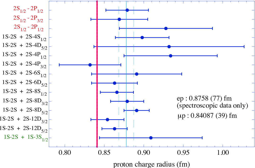
The Lamb shifts in both normal electronic as well as muonic hydrogen are sensitive to the non-point-like structure of the proton nucleus. While this effect is indeed minuscule, the ability of quantum electrodynamics (QED) to predict the energy levels of hydrogen with remarkable accuracy, together with experimental measurements of the relevant transition frequencies to around one part in 1011, results in a measurable sensitivity to the proton radius. The energies of the S-states in hydrogen are given by:
| (40) |
where is the principal quantum number, and denotes the Lamb shift of the 1S ground state which is given by QED and contains the effect of the proton charge radius, . Numerically, MHz, so the finite size effect on the 1S level in hydrogen is about 1.2 MHz. The different -dependence of the two terms in Eq. (40). permits the determination of both and from at least two transition frequencies in hydrogen. The approach taken to date has been to use the 1S-2S transition [180], which has been measured to a stunning accuracy of one part in 1015, together with one of the 2S-NLJ transitions [181, 182]. The former transition is maximally sensitive to , whereas the latter contain much smaller Lamb shift contributions, due to the scaling in Eq. (40).
In Fig. 17, we show the values of extracted from the various transition combinations. The values extracted from measurements in normal electronic hydrogen favor a value of 0.88 fm, consistent with the world-averaged electron scattering results. The discrepancy between the combined value from just electronic hydrogen alone, as obtained in the elaborate CODATA adjustment of the fundamental constants [169], and the muonic hydrogen value, is about .
The difference between the muonic hydrogen determination of the proton radius and the results obtained from either electron scattering or from electronic hydrogen transitions is highly enigmatic. The theoretical QED calculations of the portion of the Lamb shift that is not due to the finite proton size have been checked and re-checked by multiple independent groups. Also, the many measurements of the transition frequencies in electronic hydrogen are in agreement with one another. Thus, from an experimental point of view, the solution to this puzzle is not obvious at this time. On the theoretical side, there has been a significant amount of interest in this problem as well; this is discussed in more detail in Section 4.
3.4.2 Future Experiments
Experimental approaches to unraveling the proton radius puzzle break down into several distinct categories: improving the precision of the proton radius extraction from electron scattering experiments, extending the atomic spectroscopy measurements to other ions or exotic atoms, and/or determining the proton radius in elastic muon-proton scattering.
At Jefferson Laboratory, in Hall B, there is an approved experiment which aims to improve the electron scattering radius determination by extending the range from the 0.0038 GeV2 of the Mainz experiment down to 1-2 10-4 GeV2 [183]. This is indeed a challenging experiment. If the proton radius is to be determined in this experiment with similar accuracy compared to the current world-averaged result from electron scattering, then relative cross sections need to be determined at the 0.2% level. Fortunately, the large cross sections and corresponding event rates for low scattering make statistical uncertainties of 0.1% achievable. However, systematic uncertainties must also be controlled at a similar level. One of the largest sources of systematic error is the determination of the electron scattering angle; at the lowest value of the experiment, the scattering angle is only 10 mrad, and due to the severe angular dependence of the Mott cross-section at small angles, a 10 rad knowledge of the scattering angle is needed to limit shifts in the relative cross sections to 0.2%.
At MAMI, an experiment is underway that aims to measure the proton electromagnetic form factors in scattering at very low momentum transfers by using a technique based on initial state radiation [184]. The basic premise is that initial state radiation degrades the energy of the incoming electron so that the momentum transfer to the proton can be quite low. The outgoing electron angle and energy are measured as usual, and together with theoretical input, an accurate form factor can in principle be obtained at values as low as 10-4 GeV2. The full experiment ran in 2013, and the analysis is continuing.
As can be seen from Eq. (40), the determination of using transitions in hydrogen relies heavily on a precise determination of . Currently, is known from measurements of transition frequencies in hydrogen and deuterium. However, since the correlation between and is significant, new precise measurements of (at the level of a few parts in 1012) that are independent of could potentially impact the extracted value of from electronic hydrogen measurements. There are several such efforts currently underway. These include single- [185] and two-photon [186] measurements in hydrogen, as well as experiments which aim to use laser spectroscopy of neutral and ionic helium [187, 188, 189].
Noticeably, a crucial missing piece of the proton radius puzzle is a measurement of the proton radius using muon scattering; indeed, there is a proposal at PSI, the MUSE Experiment, to make just such a measurement [190]. The MUSE experiment will measure elastic scattering to a minimum of 0.002 GeV2 - about half the lower limit of the Mainz electron scattering experiment - using both positively and negative charged incident muons, so that any possible two-photon effects can be taken into account directly from the data, rather than relying on theoretical calculations. In addition, the experiment will simultaneously collect scattering data, so that the extracted proton radius from muon and electron scattering can be compared directly within a single experimental apparatus. Preliminary estimates are that the proton radius that can be extracted from muon scattering will be similar in precision to that extracted from the Mainz experiment.
3.5 Flavor Separation of Nucleon Form Factors
Charge symmetry implies that the proton and neutron wave functions are identical under the interchange of the up and down quark contributions. Measurements of asymmetries in parity non-conserving electron scattering on the proton have found that the strange quark form factors are small (see the review article by Ref. [44]). Ignoring the contributions of higher mass quarks, the proton and neutron form factors can be written in terms of the contributions from the up and down dressed quark form factors as:
| (41) |
The up and down form factors, and are defined by convention to represent the up and down dressed quark form factors in the proton. The anomalous magnetic moments of the up and down quarks can be expressed as and , respectively. The Dirac and Pauli form factors for the up and down quarks can be written as:
| (42) |
The recent precision data on in the region of between 1.5 to 4.8 GeV2 [78] and data on / to GeV2 by Ref. [33] have enabled precise phenomenological fits to the proton and neutron form factors and detailed comparison to theory predictions. This allows one to extract information about the underlying contributions of the up and down quarks to the nucleon form factors.

A calculation of the up and down quark form factors from the available proton and neutron data was done by Ref. [191]. The quark form factors were calculated to = 3.4 GeV2 by combining the measurements of / by Ref. [113, 31, 33, 111, 32, 120] with the Kelly fit [55] to , and . Fig. 18 is a plot of and / versus for the up and down quarks. The data is plotted at the of the / measurements and the error on the quark form factors is determined by the error on the / measurements. For GeV2, the dependence of both the and changes for the up and down quarks. For the up quark, and / continue to rise, while, for the down quark and / are plateauing or slightly dropping.
Another separation of the up and down form factors was done by Ref. [192]. They used and from a extraction using cross section and polarization data which included two-photon exchange contributions [157]. In addition, they added the data of Ref. [98] for at low . For the neutron form factors, they used the fit of Ref. [33] to and an updated parametrization of using the data of Ref. [72, 75, 76, 77, 78, 133]. The up and down form factors are calculated at the of the proton data and are plotted in Fig. 18. In the region of between 0.5 to 1.5 GeV2, from Ref. [192] is slightly larger than that in Ref. [191] and, correlated with that, from Ref. [192] is slightly smaller. In general, comparisons between the two different flavor separations of the form factors give a sense that the size of the uncertainty due to two-photon exchange contributions and tensions in the data sets is relatively small and does not obscure the general trends in the dependence of the up and down quarks form factors.

Great interest exists in extending the separation of quark flavors to higher . In the spirit of Ref. [191] and Ref. [192], we use the Kelly fit [55] for and while refitting and to include the data since the Kelly fit was done. The fit form for is:
| (43) |
with , and . The fit form for is:
| (44) |
with ,, , , , and . In Fig. 19, the fits are compared to the world data for the proton and neutron and . The shapes for the proton and neutron are nearly identical with the data on top on each other. A small shape difference in the proton and neutron dependence on accounts for the difference between the up and down quark’s which is seen in Fig. 18.
Using the fits the nucleon form factors, the flavor separation can be extrapolated to higher . To investigate the sensitivity of the extrapolation of the quark form factors, a different shape for can be used in calculating the quark form factors. As an example, the prediction from the Dyson Schwinger equation (DSE) model of Ref. [123] is plotted as a dash dotted line in Fig. 11. The DSE models are discussed in the theory Sec. 4.2. The up and down quark’s and from the fit using Eqs. (44) and (43) are plotted in Fig. 20 as a solid line in the region of GeV2 where data exists, then extended as a dashed line when the fit is extrapolated to GeV2. The fit shows that will have a zero crossing at GeV2 while starts to plateau above of 7 GeV2. Both and slowly drop-off above of 3 GeV2 with falling slightly faster. When the prediction from the DSE model is combined with the other form factors from the fit to calculate the quark form factor, then mainly the down quark’s form factors are modified. This is shown in Fig. 20 where the up and down quark’s and using the prediction from the DSE model are plotted as a dash-dotted line. The zero crossing in moves to lower . This demonstrates the need for precision measurements of all nucleon form factors to large . Future experiments at JLab to extend the range of the nucleon form factors measurements are discussed in Sec. 5.

4 Theoretical Interpretations of Nucleon Form Factors
We give an overview of theoretical work on nucleon electromagnetic form factors. These form factors encode the information on the structure of a strongly interacting many-body system of quarks and gluons, such as the nucleon. This field has a long history and many theoretical attempts have been made to understand the nucleon form factors. This reflects the fact that a direct calculation of nucleon form factors from the underlying theory, Quantum Chromodynamics (QCD), is complicated as it requires, in the few GeV momentum transfer region, nonperturbative methods. Hence, in practice it involves approximations which often have a limited range of applicability. Despite their approximations and limitations, some of these nonperturbative methods do reveal interesting insight into the nucleon’s structure.
Section 4.1.1 describes work simply fitting the form factors using an expansion in a transformed variable that allows convergence of a polynomial expansion for all values of . These techniques have long been used in parameterizing form factors measured in Weak decays, and part of the motivation here is to ensure a better extrapolation to obtain the slope at zero , i.e., in determining the charge radius.
Section 4.1.2 describes vector meson dominance of the photon-nucleon coupling, which in addition to being physically motivated, provides good forms for fitting the nucleon form factors. Notable here is the fact that the falling ratio was obtained from early on (although fits to the neutron form factors and form factors in the timelike region required tuning after data became available).
Section 4.1.3 uses the ideas of dispersion relations to fit the form factors. In principle, if one knew the couplings and locations of all the poles and cuts in the channels, one could calculate without further approximation the form factors at all . In practice, the information is incomplete, and what one has are good parameterizations of the form factors that obey all the necessary analyticity properties and will converge everywhere. One then uses the available data to fit parameters in these functions, and hence obtain an accurate analytic representation of the data.
Section 4.1.4 reviews the extensive work that has been done using constituent quark models to calculate the form factors. Relativity is crucial here, and many of the works use one of the Hamiltonian dynamical approaches enumerated by Dirac long ago [193]. The constituent quarks are often thought to be representatives not only for elementary quarks but also to represent not explicitly included contributions from gluons and higher Fock states, and as such may themselves have form factors that need to be parameterized. The outcome is usually a physically motivated form with parameters that need to be fit to data, and the fits in modern times are quite good for all the form factors.
QCD has chiral symmetry, and chiral symmetry in our world leads to the existence of light mesons. These light mesons can then be part of the long range structure of the nucleons, and the pion cloud models that take these degrees freedom into account are described in Sec. 4.1.5.
To simply Fourier transform the electric and magnetic form factors to obtain the charge and magnetic densities is not valid relativistically, so this door to obtaining structure information about the nucleons is closed. However, it can be shown that projections of the densities onto the transverse plane for a fast moving nucleon can be validly obtained from two-dimensional Fourier transforms of the Pauli and Dirac form factors. Work on transverse densities is described in Sec. 4.1.6.
A new approach to obtain approximate predictions for nucleon form factors is to use correspondences that have been discovered between gravitational theories in five dimension and approximately conformal field theories, like QCD when considering only the light quarks. Results from this approach are described in Sec. 4.1.7.
The Dyson-Schwinger equations (DSE) are an infinite set of equations for the vertices, propagators, and other quantities related to calculating observables from a field theory. They can be truncated with some success, and they have been well studied in QCD, with DSE results for nucleon form factors presented in 4.2.
Perturbative QCD results for the form factors are on the face of it vitiated by the measurements. The pQCD basics, and improvements to and extensions of the pQCD techniques, are reviewed in 4.3.1.
Form factors may also be obtained as integrals of generalized parton distributions (GPDs), which are the amplitudes for removing a quark from a nucleon and substituting another quark with a different momentum and possibly differing also in other quantum numbers. GPDs are important metrics of nucleon structure, and are measured in exclusive processes like or . Their consequence for nucleon form factors is highlighted in Sec. 4.3.2.
Finally, nucleon form factor results from lattice gauge theory are reviewed in Sec. 4.4. The results so far are only for the isovector form factors, but the uncertainty limits are decreasing as further work is done, and lattice gauge theory has the advantages of being really QCD and not a model of QCD, and of obtaining results that are systematically improvable.
4.1 Models of Nucleon Form Factors
4.1.1 Conformal Fits to Form Factors
There has been a lively discussion of what sorts of functions to use in fitting the form factors. Simple polynomial fits, for example, will not converge for moderate or large momentum transfers. The reason flows from the fact that the form factors are, from a mathematical viewpoint, analytic functions of their argument , except for cuts at known locations. The cuts are on the timelike side, and begin where one can have a photon to two pion transition at . A cut can be viewed as a weighted continuum of poles, so that there is a contribution to the form factor containing a factor . The weighting of this pole may be weak, but in principle its existence means that a polynomial expansion of the form factor will not converge for . It is like the expansion of the geometric series , which does not converge for .
However, it is possible to make a mapping of to another variable, denote it , where a polynomial expansion in is allowed. The trick is to find a transformation where spacelike momentum transfers all map onto the real line and timelike momentum transfers map onto the circle (in the complex -plane). Then since all poles of the form factors lie on the unit circle in , a polynomial expansion in is convergent everywhere inside the unit circle, i.e., for all spacelike momentum transfers.
This trick has been applied in the context of Weak interaction form factors, as for semileptonic meson decay, for some time [194, 195]. It has now also been applied to fitting electromagnetic form factors by Hill and Paz [162] and by Lorenz et al. [164].
The variable is given by the conformal mapping [162, 164], with ,
| (45) |
where and one can easily enough verify that the mapping has the properties stated above.
Fitting with a nonconvergent expansion can give good analytic fits to the data in any region where there is data to be fit. The danger lies in extending them outside the region where there is data. Such extrapolations can go awry, sometimes diverging wildly from physical expectation and sometimes, depending on how far one extrapolates, there may be problems that are less visible. Here enters also the proton radius question, whose evaluation from form factors requires an extrapolation from the lowest where there is data, down to . Extrapolating a fit made with an intrinsically convergent expansion is arguable safer.
The two fits made to the electromagnetic form factors using the conformal variable , however, differ in their conclusions regarding the proton charge radius. The earlier fit [162] used electron-proton scattering data available before the Mainz experiment [59] published in 2010. They found a proton radius , so their central value is closer to the CODATA value than to the muonic Lamb shift value. The other fit [164] used the 1422 data points from the Mainz experiment, and obtained fm (see also [196]).
Also in this section we may mention two recent reanalyses of world - scattering data that obtain larger proton radii, one by Sick and Trautmann [161, 197] and another by Graczyk and Juszczak [198]. The former was particularly mindful of effects of the charge density at large distances upon the charge radius, and obtained fm, including all known data; the latter used a Bayesian framework and obtained fm, albeit without including the Mainz 2010 data [59].
4.1.2 Vector Meson Dominance (VMD)
The photon has the same quantum numbers as the lowest lying vector mesons , , and . These mesons are prominent in the process at the relevant timelike values of the CM energy squared . One could hence expect that in elastic electron nucleon scattering at low spacelike momentum transfers , some or much of the behavior of the coupling could be explained by the emitted photon converting to the strongly interacting meson which then attaches to the nucleon, as illustrated in Fig. 21.

That vector meson dominance (VMD) can explain much of the low behavior of the form factors is confirmed by history. Before the [199], [200], and [201] were explicitly discovered in the early 1960’s, in reactions such as or , there were hints or predictions of the existence gleaned from the behavior of the proton form factor. Nambu [202] in 1957 suggested that the observed form factor was consistent with the existence of a vector meson intermediary, and Frazer and Fulco [203] in 1959 in a famous dispersion analysis were more explicit, even suggesting a later confirmed mass range for the meson.
A single vector meson exchange with simple couplings gives an factor, from its propagator, for the falloff of the form factor. One can obtain a high momentum falloff, in accord with observation or with pQCD, by having cancellations among two or more vector meson exchanges with different masses, or more commonly in practice by giving the vector mesons themselves a form factor in their coupling to nucleons.

An early example of a VMD fit to form factor data was given by Iachello, Jackson, and Lande [204] or IJL. They had several fits, but the one most cited is a 5 parameter fit with a more complicated propagator that the form noted above, to account for the large decay width of the meson. (The and are narrow enough that modifying their propagators gives no numerical advantage.) They in 1973 predicted the falloff of later seen experimentally, as illustrated along with some early data in Fig. 22.
The IJL work was improved by Gari and Krümpelmann [205, 206, 207] to better match the power law pQCD expectations at high , that and , but also including some corrections to the falloffs based on the running behavior of the coupling .
Further improvement in VMD fits was made by Lomon [126, 208], who included a second as the , and later also a second as the , and obtained a good parameterization for all the nucleon form factors. The first of the polarization transfer measurements [7] was available in time for Lomon’s 2001 work [126]. Lomon further tuned his fits [208] when the second set of polarization transfer data became available [9].
Viewing the form factors as analytic functions of , the VMD forms are straightforward to analytically continue to the timelike region (see, for example, Brodsky et al. [209] or Dubnickova et al. [210]), and compare to data that is now available. Workers in the field have done so, and have modified the VMD fits to give good accounts of data in both the timelike and spacelike region.
In addition, the original IJL fits [204] were not as good for the neutron as for the proton. Both the spacelike neutron form factors and timelike nucleon form factors were addressed in what may be termed IJL updates, by Iachello and Wan [211] and Bijker and Iachello [212], both in 2004. Further, Lomon and Pacetti [213] have updated and analytically continued the earlier Lomon fits in order to also give a good account of data in both timelike and spacelike regions.
The VMD fits of course are fits to existing data, and they have been regularly updated as new data appeared. It will be interesting to check the “predictions” for the neutron form factors as newer data appears. A plot of the existing situation for protons is given in Fig. 23.

4.1.3 Dispersion Analyses
Newer works here include the dispersive analyses of the nucleon form factors by workers in Bonn [164, 196, 163]. There is also work that is only slightly older by Beluskin et al. and Baldini et al. [127, 214, 215]. The works include general analyses and fits to the form factors, as well as aspects directly aimed at the resolution of the proton radius puzzle [164, 196, 163].
Dispersion relations relate the form factors in the spacelike and timelike regions. More generally, the form factors are complex functions of that are analytic except for known cuts, and the form factors anywhere can be calculated if one knows just their imaginary parts at the cuts. The cuts are all on the real axis for timelike . The cuts run from to . In practice, one cannot know the imaginary part of the form factors over this whole range, and uncertainty in knowing the form factors in the timelike region builds nonlinearly to larger uncertainty in predicting the form factors in the spacelike region, especially at higher .
At lower , one specific boon of the dispersive treatment is that the connection between the timelike and spacelike regions puts an extra constraint on the form factors and their slope at spacelike threshold. This means that the determination of the charge and magnetic radii are not purely extrapolations of the scattering data, but is an interpolation in this procedure and hence arguably more reliable.
A technique involving dispersion relations, used by both [163] and by [214], is to parameterize the imaginary part of the timelike form factors, and determine the parameters by making a least squares fit to the known spacelike and timelike data. One thereby obtains a representation of the form factors that one can use in regions where there is not yet data.
Ref. [214], published in 2006, applies dispersion relations to the ratio , with the assumption of no zeros in . They used some large-uncertainty-limit data in the timelike region, obtained from angular distributions in or the reverse, to supplement the polarization data in the spacelike region. One of the main goals was to compare to models that fit the spacelike data, especially to the continuations of those models to the timelike regions [209].
They found that there was a zero in at about GeV2 spacelike momentum transfer squared, and found that the Phragmén-Lindelöf theorem, which leads to the statement that should be the same at very large momentum transfers, whether spacelike or timelike, was satisfied, albeit with opposite signs. Many of the more purely phenomenological models differed on the latter point. This work [214] preceded the completion of the polarization experiments at the highest current [10, 101]. The dispersive aspects have not been updated in more recent works by some of the same authors, e.g. [215], but one can see that the results would not be materially changed by the newer data.
Lorenz et al. [163], in their update of [127], apply the dispersion analysis to and separately. An important improvement in the newer work [163] is that it includes the recent Mainz data [59] in its fit. A salient outcome of this analysis is that the proton charge radius comes out at a value fm, in agreement with the value found in the muon hydrogen Lamb shift measurement.
4.1.4 Constituent Quark Models
Constituent quark models (CQMs) have been used to understand the structure of baryons, beginning when quarks were first conjectured and predating the establishment of QCD as the theory of the strong interactions. Indeed, the observed spectroscopy, particularly the existence of the , played a crucial role in bringing to light the quantum number of color. In the CQM, the nucleon is a quantum mechanical ground state of three quarks in a confining potential. More generally, ground state baryons are composed of three quarks, selected from up (), down () and strange () flavors, and are described using spin-flavor wave functions and a completely antisymmetric color wave function.
Early CQMs concentrated on explaining static properties, including magnetic moments and transition amplitudes. Examples are the models of De Rújula, Georgi, and Glashow [216] and of Isgur and Karl [217]. In the latter, the quarks were in a harmonic oscillator potential, and at least at first the wave functions were nonrelativistic product wave functions, and the ground state baryons appeared as a 56-plet of . QCD by this point having been discovered, the hyperfine splittings, e.g., between the nucleon and the , were given by a one-gluon exchange potential added to the confining potential. The one-gluon exchange also generates a small tensor interaction that leads to some -state admixture into the ground state baryons. This in turn allows some non-zero electric quadrupole () and Coulomb quadrupole () nucleon to transitions, in accord with observation.
However, form factors require a relativistic treatment. At high , nonrelativistic treatments lead to form factors that are far too small compared to data. At low , the charge radius defined from the slope of the form factor has contributions corresponding to the RMS charge radius known from nonrelativistic treatments, but also has recoil terms proportional to the Compton wavelength or inverse mass, squared, of the target. The latter are absent in any nonrelativistic model, and the nucleon is light enough for this to be a problem.
A crucial question for a form factor calculation, since the nucleon must be moving after or before the interaction or both, is how the wave function in the rest frame transforms to a moving frame. This is not a trivial question, and the answer can, depending on the formalism, be dependent on the interactions binding the quarks. Formally, one needs to know how the eigenfunctions of the mass and spin operators can be viewed as unitary representations of the Poincaré group, whence it will be known how they change under Poincaré, which includes Lorentz, transformations. The generic ways this can be done were laid out by Dirac [193]. There are three forms of dynamics, which are the instant, point, and light-front forms. These differ in which generators form the kinematic subgroup of the Poincaré group. This is the subgroup whose commutators do not involve the interactions among the constituents. The Poincaré group has ten generators, four space-time translations (momentum operators), three spatial rotations, and three boosts. In a given representation each of these may be kinematical or interaction dependent, or dynamical, meaning dependent on the specifics of the interaction potential. The latter cannot usually be dealt with in an exact way, but must be dealt with approximately or numerically in a practical calculation.
The point form has all boosts and rotations kinematical, meaning that as operators in a field theory they can be written out without having to know the interaction Lagrangian or interaction Hamiltonian. Straightforwardly, the angular momenta and Lorentz boost are the same as in the free case. However, all four components of the momentum operators are interaction dependent in this case.
The instant form has the rotation operators and space components of the momenta kinematical. Eigenstates of the angular momentum are then easy to construct. However, the time component of the momentum, or Hamiltonian, and the boosts are dynamical. Boosts, then, require knowing and including effects of the interaction in order to ascertain important infomation, e.g., the momentum space wave function, of the boosted state.
The light-front form has seven kinematical generators. This is the maximum possible. The three dynamical generators are one component of the four-momentum operator (for which the mass operator obtained from may be substituted) and two light-front transverse rotations (or light-front transverse boosts, meaning here two particular linear combinations of the two ordinary transverse rotations and the two ordinary transverse boosts). Light-front calculations have the advantage that states can be easily and exactly transformed from one frame to another the using the (kinematic) longitudinal boost, and the two kinematic light-front transverse rotations (the linear combinations orthogonal to the one previously mentioned). However, light-front calculations have the disadvantage that states of definite angular momentum are difficult to construct because the rotation operators are interaction dependent.
A calculation of the form factors also requires knowing the electromagnetic current operator. It is usually assumed that the photon only interacts with one quark in the nucleon.
The relative ease of exactly transforming states from the frame where the wave functions are calculated or otherwise given, to any other frame, makes the light-front form attractive for form factor calculations. The light-front form in this context was introduced by Berestetsky and Terentev [218, 219], and later developed by Chung and Coester [220]. In these calculations one begins with some wave function that has been developed in CQMs designed to study the baryon spectrum. The light-front form of the wave function is obtained by a Melosh or Wigner rotation of the Dirac spinors for each quark. These come about because the usual CQM models use spinors that in momentum space are obtained from rest spinors by a direct boost, while the light-front spinors are obtained by a longitudinal boost followed by a kinematical light-front transverse boost. Undoing one and then applying the others leads to the same momentum, but leaves a residual rotation that does not affect the momentum, but does affect other quantities such as the spin. While the Melosh rotation is not difficult conceptually, the expressions it leads to are tedious to write out.
If, in addition, one calculates in the so-called light-front (or Drell-Yan) frame characterized by , then momentum conservation ensures that the current matrix elements connect only states whose Fock components have the same number of constituents. There are, for example, no matrix elements connecting to states, so that a consistent calculation can be done using only three-quark states.
Chung and Coester [220] used Gaussian wave functions. They did obtain a falling ratio. This apparently [128] is a feature shared by many relativistic calculations and occasioned by the Melosh transformation. However, the form factors fell far too fast at large . Schlumpf [221, 222] used instead a wave function with a power law falloff, fitting parameters in his wave function to static baryon properties. The high falloff was now in line with data, including some at that time new neutron data [72], and also showed a ratio that fell more slowly than , in qualitative agreement with later data.
French, Jennings, and Miller [223, 224] focused on the effects of the nuclear medium upon the form factors, but also calculated the form factors of single free nucleons. They followed the work of Schumpf [221, 222] and similarly found a decreasing ratio, obtaining a zero between 5 and 6 GeV2 for .
Improvements in the detailed quality of the fit can come by introducing Dirac and Pauli form factors for the quarks. This can be justified by arguing that nucleons are not just bound states of three quarks, but have further constituents in the form of gluons and quark-antiquark pairs. Modeling the nucleon with three quarks means the constituent quarks are also representing the additional components present in a complete Fock space expansion of the nucleon, and this gives them an effective structure represented by the quark form factors. This viewpoint was taken by Carderelli et al. [225, 226] (plus further references contained in the latter) to produce good fits to both the proton and neutron form factor data then available. They used the light-front formalism and quark wave functions obtained from a potential of Capstick and Isgur [227], and made the point that the one-gluon exchange is crucial to obtaining sufficient high momentum components in the wave function to explain the form factor data.
A different starting wave function, now in the context of the point form formalism, appears in the hypercentral constituent quark model of De Sanctis, Santopinto, and others ([228, 229] and references therein). The feature here is that the confining potential is treated as a function of an average separation defined by the RMS sum of the quark positions, relative to the CM, and there is also a term to give the hyperfine splitting. Parameters of the potential are fit to the baryon mass spectrum. With the inclusion here also of form factors for the constituent quarks, good fits are obtained for the nucleon form factors, with updates [229] succeeding the latest polarization transfer results [10].
A comparable amount of high-momentum components in the nucleon wave function was obtained in the Goldstone-boson-exchange (GBE) quark model [230, 231]. This model relies on constituent quarks and Goldstone bosons, which arise as effective degrees of freedom of low-energy QCD from the spontaneous breaking of the chiral symmetry. The resulting CQM assumes a linear confinement potential supplemented by a quarkÐquark interaction based on the exchange of pseudoscalar Goldstone bosons, which is the source of the hyperfine interaction. It was shown [230, 231] that the GBE CQM yields a unified description of light- and strange-baryon spectra. The GBE CQM was used in [232, 233] to calculate the nucleon e.m. form factors in the point-form. The neutron charge radius is well described in this model and is driven by the mixed-symmetry component in the neutron wave function. In contrast to the light-front calculation [226, 234], it was found that when performing a point-form calculation of the nucleon e.m. form factors at larger within the impulse approximation, i.e. considering only single-quark currents, a surprisingly good overall description of the nucleon e.m. form factors can be obtained, using point-like constituent quarks only. When looking at details of Refs. [232, 233], the agreement is worse though for which is underpredicted at larger , and the ratio of is overpredicted at larger , see Fig. 24. Similar findings have also been obtained in the point-form calculation of [235] for the one gluon exchange CQM. The overall success of the point-form result using point-like constituent quarks was attributed in [232, 233, 235] to the major role played by relativity. Such a finding is remarkable in view of the expected finite size of the constituent quarks, as discussed above.
An explanation for the above finding for the nucleon e.m. form factors in the point form, using the single-quark current approximation, has been suggested by Coester and Riska [236]. When the spatial extent of the three-quark wave function is scaled (unitarily) to zero, both instant and front forms yield form factors independent of the momentum transfer. Therefore, to reproduce the experimental fall-off of the nucleon e.m. form factors at large momentum transfers requires the introduction of constituent quark form factors. In contrast, when the wave function in point form is scaled unitarily to zero (so-called point limit), a non-trivial scaling limit is obtained for the form factors, depending on the shape of the wave function. At high values of momentum transfer, the scaled form factors decrease with an inverse power of the momentum transfer. The power is determined by the current operator and is independent of the wave function. An explicit comparative calculation of the baryon e.m. form factors between the three different forms was performed in [237] using a simple algebraic form for the three-quark wave function, depending on two parameters. It was verified that a qualitative description of the nucleon form factors data demands a spatially extended wave function in the instant- and front-form descriptions, in contrast to the point-form description which demands a much more compact wave function.
A manifestly covariant CQM calculation within the Bethe Salpeter formalism and using an instanton-induced interaction between quarks has been performed by Merten et al. [238]. Although this model reproduces the baryon spectrum, it can only qualitatively account for the dependence of the nucleon e.m. form factors.
Another type of covariant CQM calculation was done by Gross, Ramalho, and Peña [239], partly based on earlier work of Gross and Agbakpe [240], avoiding questions of dynamical forms by staying in momentum space. They use a covariant spectator model, where the photon interacts with one quark and the other two quarks are treated as an on-shell diquark with a definite mass. They too take the view that the constituent quark includes, at least at lower , effects from higher Fock states and so the quark itself should have a form factor, including the possibility of nonzero quark anomalous magnetic moments. They note, as others have, that obtaining a good fit to the neutron electric form factor requires isospin breaking. Since they use VMD forms for the quark form factors, the difference between the (isospin-1) and the (isospin-0) couplings is one sufficient way to obtain this. They obtain forms with parameters that they fit to the data. Their fit from the 9-parameter “model IV” is quite precise.
Of interest, especially noted in [239] although perhaps somewhat relaxed in [241], also by Gross et al., is that only -state quark wave functions are needed to obtain good fits to the form factors. Other work (the article of Brodsky and Drell [242] is an early example) argues, on the other hand, that nonzero angular momenta are necessary for fitting the form factor data. This can be a difference in organization of the calculation. Looking in particular at the magnetic moments, if there are only -states, the anomalous magnetic moments of the nucleons can only come from intrinsic anomalous magnetic moments of the quarks, which can be nonzero if quark form factors are allowed; whereas if the quarks are all elementary particles their anomalous magnetic moments are zero, and higher Fock states or nonzero orbital angular momenta are needed to produce the observed magnetic moments of the nucleons.

4.1.5 Pion Cloud Models
In nature, the up and down quarks are nearly massless. In the exact massless limit the QCD Lagrangian is separately invariant under rotations in flavor space of the left handed and right handed quarks. I.e., there is invariance under a chiral symmetry group . Parity is also a symmetry of the Lagrangian, and fully compatible with the chiral symmetry, and so it would seem that for any state of QCD, there would be an equal mass state of opposite parity. However, parity doubling is not seen in nature. Instead we find the alternative, which is that there exist massless negative parity scalars, the Goldstone bosons. For two quark flavors, there are three Goldstone bosons, the pions, which acquire a mass in nature because of the symmetry breaking due to the quark masses. Since the pions are light, they dominate the long distance behavior of the nucleon wave functions, and have a potentially important effect on the low-momentum transfer behavior of hadronic form factors. Hence one can improve the constituent quark models by including pionic degrees of freedom.
One early improvement to constituent quark models was in the context of the bag model of hadrons, where a number of workers, in or about 1980, including Brown and Rho [244], Jaffe [245], and Thomas, Théberge, and Miller [246] secured the chiral symmetry of the model by including coupling to pions. The vision was then of quarks within the boundary of the bag and pions without, and the model was called the Cloudy Bag Model. However, states of the bag model are expressed in coordinate space as set of independent particle wave functions for each quark. Turning these states into momentum eigenstates is not a trivial problem in general, because there are center-of-mass fluctuations that must be removed, and momentum eigenstates are needed to discuss the form factors. Additionally, the bag has a simple spherical boundary in the rest frame, and it must be understood how the states alter under Lorentz transformation in order to make accurate form factor calculations for nucleons. Hence some time passed before Lu et al. in 1998 [247] calculated nucleon electromagnetic form factors in the cloudy bag model. They used the Pierels-Thouless formalism and a plausible hypothesis for the effects of Lorentz transformations (details in [247]), and obtained a good description of the nucleon electromagnetic form factors for GeV2.
Miller extended the calculation to larger using a light-front version of the cloudy bag model calculation [128]. Starting from constituent quarks [224], using the Schlumpf wave function instead of bag wave functions for the quark core, Miller calculated the effects of the pion cloud through one-loop diagrams. The model gives a relatively good overall account of the form factor data at both lower and higher .
The cloudy bag model is one chiral quark model which treats the effect of pions perturbatively. Other quark models which calculated nucleon electromagnetic form factors using perturbative pions can be found e.g. in the early works of [248, 249, 250], as well as in the already discussed works of [230, 231]. Recently, the above chiral quark models where pions are included perturbatively have been improved in [251]. This work extends a previous work of [252] by dynamically dressing bare constituent quarks by mesons to fourth order within a manifestly Lorentz covariant formalism. Once the nucleon and hyperon magnetic moments are fitted, other e.m. properties, such as the nucleon e.m. form factors at low momentum transfers, follow as a prediction. It was found in [251] that the meson cloud is able to nicely describe the form factor data in the momentum transfer region up to about 0.5 GeV2. To extend the calculations to larger , a phenomenological approach has been adopted in [251] by introducing bare constituent quark form factors which were parameterized in terms of 10 parameters. Such parameterization makes it plausible to simultaneously explain the underlying dipole structure in the nucleon e.m. form factors as well as the meson cloud contribution at low which results from the underlying chiral dynamics. In a later paper [253], a model calculation for the bare constituent quark form factors has been performed and applied to the electromagnetic properties of the transition, and also of the Roper transition [254]. The latter paper also includes updates of that group’s fits to the nucleon form factors.
When pion effects dominate nucleon structure, their effects have to be treated non-perturbatively. A nonperturbative approach which has both quark and pion degrees of freedom and interpolates between a CQM and the Skyrme model (where the nucleon appears as a soliton solution of an effective nonlinear pion field theory) is the chiral quark soliton model (QSM). As for the Skyrme model, the QSM is based on a expansion (with the number of colors in QCD). Its effective chiral action has been derived from the instanton model of the QCD vacuum [255], which provides a natural mechanism of chiral symmetry breaking and enables one to generate dynamically the constituent quark mass. Although in reality the number of colors is equal to three, the extreme limit of large is known to yield useful insights. At large the nucleon is heavy and can be viewed as “valence” quarks bound by a self-consistent pion field (the “soliton”) [256]. A successful description of static properties of baryons, such as mass splittings, axial constants, magnetic moments, form factors, has been achieved (typically at the 30 % level or better, see [257] for a review of early results). After reproducing masses and decay constants in the mesonic sector, the only free parameter left to be fixed in the baryonic sector is the constituent quark mass. When taking rotational () corrections into account, this model achieved a qualitative good description of the nucleon electromagnetic form factors in the range GeV2, using a constituent quark mass around MeV [258]. The chiral soliton model obtained a decrease of the ratio with increasing already in the late 1990’s.
Holzwarth [259] extended the chiral soliton model by including the and meson propagators for the isovector and isoscalar channels, respectively. Furthermore, to extend the range in of the predictions, he uses a relativistic prescription to boost the soliton rest frame densities to the Breit frame. Such prescription is also used to extract radial charge and magnetization rest frame densities from experimental form factors, as will be discussed in Sect. 4.1.6. Using 4 fit parameters (one effective boost mass and three free parameters to fix the couplings of and mesons), the model was found to provide a good account of the detailed structure of the nucleon e.m. form factors in the low region. In particular, for it predicts a decreasing ratio in good agreement with the data. At larger , the boost prescription gives a reasonably good account of the data (except for ) and predicts a zero in around 10 GeV2. Due to the uncertainty introduced from the particular choice for the boost prescription, the high behavior (for larger than about ) of the e.m. form factors is however not a profound prediction of the low-energy effective model.
Cloët and Miller [260], in addition to fitting the electromagnetic form factors with a quark plus pion cloud model, have the further goal to accurately reproduce the spin fraction of the proton that comes from quark spin. It will be remembered that the EMC collaboration found that little of the proton spin came from quark spin, and a more modern analysis [261] gives the quark spin fraction of the proton spin as % (for and ). The Cloët-Miller model uses a light-front formalism with a quark-diquark system accounting for 71% of the nucleon state, by probability, plus a quark-diquark core with a pion accounting for the rest. Gluons are not explicitly included. They have 10 parameters, which they fit to the electromagnetic form factor data, obtaining a good representation of the data and/or the Kelly fit thereto. They have a zero of at GeV2. The total quark plus diquark spin they obtain is 36.5% of the proton’s , in fine accord with expectation.
4.1.6 Transverse Densities
Nonrelativistically, form factors and charge distributions are Fourier transforms of each other. Relativistically, this is no longer true, because of quandaries in transforming the nucleon wave function from one reference frame to another. In terms of the charge or magnetic radius this leads to additive terms that may be called recoil terms, proportional to with coefficients that are not trivial to calculate. For heavy targets, these terms may be ignored, but the nucleon is light enough that precision work cannot proceed nonrelativistically. One cannot obtain accurate spatial images of the nucleon charge or magnetic densities by just Fourier transforming the charge or magnetic form factors.
However, one can obtain kinematically correct, and accurate to the same level that the input data is accurate, charge distributions if one is willing to adopt a new viewpoint. The viewpoint is that of a light front moving towards a nucleon, or equivalently of an observer viewing a nucleon approaching at nearly the speed of light. The charge density that will be seen is two dimensional, or the 3D charge density of the nucleon projected onto a plane transverse to its direction of approach. Additionally, the charge density that will be seen is not the charge density obtained from the electromagnetic current component , but rather densities coming from .
Typically one chooses the z-direction as special, choosing it along the direction , where and ate the incoming and outgoing nucleon momenta, and further arranges the frame so the photon momentum has , and its transverse (lying in the plane) momentum is denoted . The charge density projected onto the transverse plane is shown in works of Burkardt and of Miller and of others [262, 263, 264, 265] to be
| (46) | |||||
where is the position in the plane relative to the nucleon’s CM, is the (light-front) helicity, and the longitudinal and transverse components of the incoming and outgoing nucleon’s momenta are indicated separately. For the density of an unpolarized nucleon one finds, following Miller [263], that
| (47) |
where , is the Bessel function, and is the Dirac form factor. Further, if one polarizes the nucleon transversely in the -direction, one obtains [264],
| (48) | |||||
where is the azimuthal angle of , and is the Pauli form factor.
The result for the unpolarized density distribution of the proton is not startling and is not shown here, but the result for the neutron is quite striking [263]. The neutron charge density is found to be negative near its center as shown in Fig. 25; it had long been known to be negative far from the center.

For a transversely polarized neutron, one finds a charge separation as shown in Fig. 26, based on figures in [264]. The upper panel shows the difference between the charge densities of the polarized and unpolarized neutron. One sees negative charge above and positive charge below. The lower panel gives similar information by comparing the polarized and unpolarized charge distributions along a single line, the -axis. (One should know that time reversal invariance forbids an electric dipole moment for a stationary elementary particle, but for a moving particle the electric dipole moment is given by , where is the velocity of the particle and is its magnetic moment.)


4.1.7 Correspondences with Higher Dimensional Theories
A recent, exotic, and interesting way to obtain approximate QCD results is to use the anti-de Sitter space/conformal field theory (AdS/CFT) correspondence, initiated by Maldacena [266], where the most relevant approximately conformal field theory is QCD and we talk of the AdS/QCD correspondence, where early applications were made by Erlich et al. [267]. The idea is that some string theory in ten dimensional space has a symmetry that is divided so that for five dimensions we are and remain in the ground state in those dimensions, and the theory in the other five dimensions mimics a gravitational theory in a five dimensional anti-de Sitter space, or AdS5. The AdS5 possesses a symmetry, which is important because it is the same symmetry possessed by a conformal (in practice, a theory with all masses zero) field theory in four dimensions. One can exploit the sameness of the symmetry group to find numerically viable relations between the solutions to the gravitational theory in five-dimensions and the conformal field theory in four-dimensions. For an extensive review, see [268].
Since QCD is not a conformal theory, maintaining a correspondence requires also breaking the symmetry of the AdS space, which in practice is done either with the hard wall model, where the AdS space is cut off at long distances in the fifth dimension, or by the soft wall model, where an extra potential is introduced that suppresses long distance propagation in the fifth dimension.
Much of the work on individual particles has focused on the bosonic sector, studying both quarkic hadrons and glueballs of various spins, and obtaining masses, decay constants, and charge radii. The actual correspondence is between operators in the four-dimensional space, such as the electromagnetic current or the energy momentum tensor , and fields in the five-dimensional space with corresponding quantum numbers, such as a vector field or the metric . Results can be compared to experiment at the few times 10% level [268].
Obtaining results for fermions is more involved than for bosons. One approach is to build from the bosonic sector, and treat the fermions as Skyrmions within that model [269, 270]. Another approach is to begin in AdS with fundamental fermions that interact with the AdS gravitational background [271, 272, 273, 274, 275, 276, 277, 278]. In this version the five-dimensional Lagrangian is still relatively simple. It has terms for gravity (the scalar curvature and the cosmological constant terms) and for vector fields, and the terms for the fermions are simple given the context of interactions with gravity and the vector field,
| (49) |
for the hard wall version of the model, and the covariant derivative is , where is the vector field which will be dual to the electromagnetic current when we make the correspondence. The indices , , , etc., each run over five values as appropriate to the five-dimensional space. In the above Lagrangian, gravity enters via the metric and is seen in its determinant and also in the spin connection , which will not be given in detail here.
As an example, results obtained using the AdS/CFT correspondence for the proton electromagnetic form factors by Abidin et al. [276] are shown in Fig. 27 for both the hard wall and soft wall models.


4.2 Dyson-Schwinger Equations and Diquark Models
The Dyson Schwinger equations (DSE) are generically a non-perturbative approximation for obtaining results for a field theory, in the present case QCD. The equations are, in principle, an infinite set of coupled integral equations. In practice, they must be truncated, in a way that preserves all symmetries of QCD, in order to proceed with any calculation. For a general DSE review, see [280].
One accomplishment of the DSE follows the solution for the full quark propagator, represented in momentum space as
| (50) |
where the normalization and the mass become functions of momentum because of interactions. With relatively simple truncations and modeling of the QCD interactions, the DSE obtain a mass function in good agreement with lattice calculations. The mass is several hundred MeV at small and falls smoothly to the small values at large that one might expect in perturbation theory.
Also early in the DSE program is building a model of the quark-quark and quark-antiquark interactions that will reproduce data on, among other quantities, the pion mass and decay constant.
One then uses the same quark-quark interactions developed in meson studies to obtain a three quark wave function model for the nucleon by solving the three-cody Fadeev equations. There arise significant diquark contributions, i.e., significant quark-quark correlations, which have a strong effect on the form factors one obtains. Since the quarks in this model are dressed, many of their features are different from expectations for pointlike fermions. One finds in particular large quark anomalous chromomagnetic moments, which affect the quark-gluon interactions, which lead to large quark anomalous magnetics moments in the quark-photon interactions, which in turn are needed to obtain good fits to the nucleon electromagnetic form factor data.
The theoretical DSE results, from the work of Cloët, Roberts, and others [281, 282, 283], show a falloff of the / ratio similar to what is seen in the data; see Fig. 28.

Qualitatively, the behavior of the form factors in the DSE approach is related to the behavior of the mass function . At lower momenta, where the mass function is far from its perturbative or current quark value, the Pauli form factor is also large compared to its perturbative value and is falling more slowly than perturbation theory predicts. (For reference, perturbative QCD predicts a power law falloff for at large , and a falloff for . ) Hence one can get a zero in ,
| (51) |
and hence a falloff in the ratio .
For the newer DSE calculations reported by Segovia et al. [284], the zero in is at GeV2. If the mass function fell to its low perturbative value more quickly than it does, the quarks would behave more like free quarks, and the value of the Pauli or anomalous magnetic moment, form factor would be small as well as quickly falling. In such a case, the zero of would be pushed to higher values of or possibly not occur at all [284].
We may mention that models based on the Dyson-Schwinger equations, as well as many of the other models discussed, do extend to form factors for other hadronic reactions, such as the electromagnetic transition [284, 285]. The result for the ratio of the electric and magnetic transition form factors for this process, , turns out to be small in the DSE approach, even at momentum transfers above 5 GeV2, in accord with experimental data. The perturbative QCD result, that , may well ensue, but only at momentum transfers well above those now experimentally accessible.
4.3 Links between Deep-Inelastic Scattering and Nucleon Form Factors
4.3.1 Perturbative QCD Inspired Models
Perturbative QCD (pQCD) predicts the scaling behavior of the nucleon electromagnetic form factors are high . The predictions were given by Brodsky and Farrar [286, 287] and by Matveev, Muradyan, and Tavkheledze [288], and pQCD not only predicts the scaling behavior of each amplitude, but also predicts that the leading amplitude is the one where the hadron helicity is maintained in the interaction. A photon of high sees the nucleon as a set of three parallel moving quarks, one of which absorbs the high momentum photon, whose momentum is brought in from a sideways direction. In order to reconstitute the proton, the momentum must be shared out by two hard gluon exchanges, so that one also has three parallel moving quarks in the final state, as illustrated in the Fig. 29.

The overall hard amplitude can be factored [289, 290, 291, 292, 293, 294] as a product of a hard scattering amplitude that takes three parallel moving quarks into three parallel moving quarks, and two distribution amplitudes (DA) that specify how the longitudinal momentum of the nucleon is divided among the quarks. Each gluon carries a virtuality proportional to (and there are also factors from each of the internal quark propagators, factors of from each of the thoroughgoing quark lines, and a involved in the definition of ), leading to a pQCD prediction that the helicity conserving Dirac form factor will fall like , with possible factors, at high . The Pauli form factor requires a helicity flip between the final and initial nucleon, which in turn requires, thinking of the quarks as collinear, a helicity flip at the quark level, which is suppressed at high . The result is a prediction that will fall like at high . Hence, and will both fall like asymptotically.

We can see how well pQCD predicts current electromagnetic proton form factor data by examining Fig. 30. The figure shows data up to 10 GeV2 for (upper panel) and (lower panel). For , it appears that the curve is flattening out, as pQCD would predict, and indeed there is data for up to 31 GeV2 to corroborate this. However, for , where there is no further data currently, the existing data does not match the simple pQCD expectation.
The data show that falls slower than with increasing . Belitsky, Ji, and Yuan [295] investigated the assumption of quarks moving collinearly with the proton, which underlies the pQCD prediction. They have shown [295] that by including components in the nucleon light-cone wave functions with nonzero quark orbital angular momentum projection, they obtain a behavior at large , with a non-perturbative mass scale. (Refs. [296, 297] also discuss using quark orbital angular momentum to get a ratio which drops slower than with increasing .) With around GeV [295], the data for agree with such double-logarithmic enhancement, as seen in Fig. 31, where it may be noted that the higher data was obtained after [295] was published. The arguments of [295] do still rely on pQCD, and it remains to be seen if still higher data will continue to support this amended prediction.


Hard scattering is calculated as if all three quarks are moving fast. An alternative is that one quark carries nearly all the nucleon’s momentum, and the other two quarks are soft. It is not necessary to transfer momentum to the soft quarks before reconstituting the proton. Nesterenko and Radyushkin [298] point out that the hard scattering mechanism requires the exchange of two gluons, each of which brings in a suppression factor . One therefore see that the hard scattering mechanism for could be numerically suppressed relative to the soft term, also called the Feynman mechanism; see also [299, 300].
Early on, Duncan and Mueller [301] showed that the soft or Feynman process also gave a falloff, with logarithmic corrections, for the Dirac form factor . This has been taken up more recently by Kivel and Vanderhaeghen [302, 303], who were able to show that also for the Feynman process, a type of factorization was possible, where the second step is given by a process independent kernel that transfers momentum among the initially all finite momentum fraction quarks to make two of them soft, as in Fig. 32. They also considered the Pauli form factor , not with the same success in proposing a factorization theorem, but showing at high enough also for the soft process.

We shall also mention work where the soft contribution was evaluated within the light-cone sum rule (LCSR) approach of Braun et al. [146]. Using asymptotic distribution amplitudes for the nucleon, the LCSR approach yields values of and which are within 20% compatible with the data in the range – GeV2. The electric form factors however were found to be much more difficult to describe, with overestimated, and near constant when using an asymptotic nucleon distribution amplitude. Only when including twist-3 and twist-4 nucleon distribution amplitudes within a simple model, is a qualitative description of the electric proton and neutron form factors obtained. Such higher twist components hint at the importance of quark angular momentum components in the nucleon wave function.
4.3.2 Generalized Parton Distributions
Generalized parton distributions (GPDs) represent an amplitude for removing a quark from a nucleon and replacing it with another quark with a different momentum, and possibly also with different spin projection and flavor. These amplitudes can be measured in virtual Compton scattering, , or in meson electroproduction, e.g., . The momenta are indicated, with , the virtuality , and will be the momentum transfer to the nucleon. A diagram for the virtual Compton process is shown in Fig. 33, in a diagram where both photons interact with the same quark. The upper part of the diagram is to be calculated perturbatively, and the lower part of the diagram is given by the GPD. For “deep” virtual Compton scattering, where , it has been shown that the dominant contributions are given by diagrams like the one shown, and that one can separate or factor the perturbative process specific stage of the interaction from the non-perturbative process independent part (see [304, 305, 306, 307, 308, 309] for reviews and references).

Further notation is that is the average nucleon momentum, is the average momentum of the quarks entering and leaving the nucleon, is the light-front momentum fraction defined from , and the asymmetry between the quark momenta is given by the skewedness . In the high limit, one can show that is related to the Bjorken variable by , where .
GPDs were introduced by Ji [310] and by Radyushikin [311]. Formally, in the notation of Ji [310]11 1 A gauge link P, ensuring color gauge invariance, is tacit. and in a frame where and are collinear with in the positive -direction, one obtains the GPDs from,
| (52) |
where is the quark field for flavor and is the nucleon Dirac spinor. The matrix element is non-perturbative and is given in terms of two functions and for each flavor . There is a similar matrix element with operator and two further, polarized, GPDs and .
The notation is such that positive momentum fractions correspond to quarks and negative ones to antiquarks. Hence in , the fermions leaving and entering the nucleon are both quarks. Also possible is that both are antiquarks (), or that there is a quark-antiquark pair.
GPDs enter this review because of their relation to form factors. An integral over on the LHS of Eq. (52) forces both quark fields to be at the same point, as in the matrix elements of the electromagnetic current. One can show that the matrix elements have support for , and that
| (53) |
where the nucleon form factor are given in terms of the quark flavor form factors in the expected ways,
| (54) |
where and are specifically for the proton.
These relations allow us, if we have complete measurements or good models (the latter is more the case at present) for the GPDs, to obtain the electromagnetic form factors from them. Alternatively, the measured form factors can be used as constraints upon GPD models.
An example of model GPDs is the modified Regge parameterization for and that was proposed by Guidal et al. [312],
| (55) |
depending on 3 parameters. The Regge slope is determined from the Dirac radius, and two parameters and , entering the GPD , ensure that the limit of has extra powers of compared to that of . This results in a proton helicity flip form factors which has a faster power fall-off at large than , as observed experimentally.


In Fig. 34, the proton and neutron Sachs electric and magnetic form factors are shown. One observes that the 3-parameter modified Regge model gives a rather good overall description of the available form factors data for both proton and neutron in the whole range, using as value for the Regge trajectory = 1.105 GeV-2, and the following values for the coefficients governing the behavior of the -type GPDs: = 1.713 and = 0.566. Note that a value corresponds to a asymptotic behavior of the ratio at large . The modified Regge GPD parameterization allows one to accurately describe the decreasing ratio of with increasing , and also leads to a zero for at a momentum transfer of GeV2.
4.4 Lattice QCD Calculations of Nucleon Form Factors
Strictly speaking, lattice calculations of nucleon form factors are currently available only for the isovector form factors.
Isoscalar form factors require calculations of disconnected diagrams, which are diagrams with quark loops not connected to the quark lines emanating from or ending on the lattice nucleon source or sink. There are gluons that attach the quark loops to the valence quarks, but these are not indicated in lattice diagrams, hence the phrase “disconnected.” Contributions from the disconnected loops require computer time intensive calculations, and remain undone. However, the disconnected diagrams contribute equally to proton and neutron, so the isovector case can be considered without them.
A review including lattice form factor results up to 2010 is available in [315], and newer lattice form factor results are reported in [316, 317, 318].
The new calculations reported in Green et al. [318] have pion masses from 373 MeV down to close to physical 149 MeV. The latter also strove to reduce contamination from excited nucleons. They analyze their lattice data using three methods which they call the standard ratio method, the summation method, and the generalized pencil-of-function method (GPoF), with varying outcomes. The best results, judged by comparison to data as represented by one of the standard fits [319], come from the summation method. Here agreement with experimental data is good for both and in the region considered, which is from scattering threshold up to about 0.5 GeV2, with uncertainty limits about at of GeV2.
The works of Alexandrou et al. [316] and Bhattacharya et al. [317] have pion masses in the 213–373 MeV range, and quote results for somewhat higher . For above about GeV2, their isovector form factors results tend to be 50% or so above the data for (or ), with uncertainties indicated at about 10%. For (or ) the results are closer to data . The authors of these works do point out that the lattice treatments with these pion masses are all consistent with each other.
One may specifically focus on nucleon radii calculated from lattice gauge theory. In the future, it may be possible and desirable to calculate using a dedicated correlator which gives directly the slope of the form factor at zero momentum transfer. Finding such correlators by taking derivatives of known correlators is suggested and studied [320] for lattice calculations of form factors at points where the Lorentz factors they multiply go to zero. Applications in [320] are to form factors for semi-leptonic scalar meson decay, and to hadronic vacuum polarization corrections to the muon .
At present, lattice calculations of nucleon radii proceed by calculating the form factor at several non-zero , fitting to a suitable form, typically a dipole form, and finding the radius by extrapolating to zero . Truly complete results are available only for the isovector nucleon. Ref. [318] presents a plot of radius results for lattice calculations at various pion masses. They use the Dirac radius, obtained from the slope of , rather than the charge radius obtained from , but these are related by, using the proton as an example,
| (56) |
where is the isovector anomalous nucleon magnetic moment. Hence, given the great accuracy of the magnetic moment measurements, one knows the Dirac radii to the same accuracy as the charge radii.
The great interest is to obtain sufficient accuracy from the lattice results to be able to adjudicate between the electron and muon measured values of the isovector charge or Dirac radii. The electron measured isovector radius is straightforward to look up, the muon measured value of the Dirac or charge radius is for now a defined quantity obtained by using the electron value for the neutron radius-squared. Using the summation method, Ref. [318] obtains, by extrapolation to the physical pion mass, a value of the isovector Dirac radius between the muonic and electronic results, with uncertainties that accommodate both at about the one standard deviation level. However, using the GPoF or ratio method gives a smaller , on the order of the value from the summation method.

One may say there is opportunity for further work. An uncertainty of 1% or less for the proton alone is needed for a lattice calculation to impact the proton radius puzzle. Two extrapolations are needed to obtain the charge radius for a physical nucleon. On is in the lattice pion mass, commented upon above. The other is in . Currently on the experimental side, the lowest from scattering data is about GeV2, and there are experiments planned or running to reduce this number. Further there are discussions, alluded to in Sec. 4.1.1, regarding the best fit forms to use for the extrapolation. Currently on the lattice, represented by Ref. [318], the lowest is about GeV2, and the fit to the lattice data is only done using a simple dipole form.
And of course one wants the isoscalar as well as the isovector form factors. However, a challenge involving just the isovector form factors, albeit at a higher than lattice form factor results currently display, is to obtain the zero in the isovector that is visible in the fits to the experimental data shown in Fig. 35.
5 Outlook
The experimental and theoretical status of the nucleon form factors were reviewed extensively in the 15 years following publication of the results of the first recoil polarization experiment at Jefferson Lab [7] for the proton. Chronologically these reviews include Gao [321], Hyde-Wright and de Jager [322], Perdrisat et al.[323], Arrington et al. [324], Cloët et al. [123], Arrington et al. [325], Perdrisat and Punjabi [326] and S. Pacetti et al. [327]. The completion of the GEn(1) and GEp(3) experiments, which reached a maximum of 3.4 and 8.4 GeV2 respectively, has brought the field into previously unexplored regions of four-momentum transfer squared, and correspondingly, generated a burst of theoretical investigations along old and new paths.
The proton form factors were originally introduced in the approximation of non-relativistic scattering, as the three-dimensional Fourier transform of the charge density [23, 328]. However the proton recoil implies that the electron is interacting with a moving charge distribution. Already for =0.25 GeV2, the recoil proton relativistic boost factor is 1.1, corresponding to . The argument that form factors are Fourier transforms of nucleon density in the Breit frame had to be abandoned, as this frame’s velocity in the Lab frame is significantly different for every .


Changes in our view of the structure of the proton are many. For example, the proton in its ground state is not necessarily spherically symmetric, but can show a typical multipole shape, when referred to the spin direction of one of its quarks (constituents) relative to the nucleon spin orientation [329]. Also, the wave front or infinite momentum frame charge and magnetization densities are invariant, two-dimensional transverse distributions which are drastically different from the non-relativistic ones [329, 330].
A selection of model predictions for the form factor ratios and is shown together with the data obtained in double polarization experiments at JLab and in other laboratories in Fig. 36. These two figures emphasize the importance of future experiments which will establish whether either ratio does, or does not cross zero near 10 GeV2. Whereas for , all model predictions discussed in this review anticipate a zero crossing somewhere above 9 GeV2, for only the calculation based on the Dyson-Schwinger equations predict such a zero crossing in the 10 GeV2 region of .
A recent development has been the calculation of the flavor separated form factors of the ”dressed” quarks from simple linear relations between the nucleon form factors, assuming charge symmetry applied to the data available. The dressed up and down quarks have significantly different form factors [123, 191, 331, 332, 282, 192]. Nucleon form factors determine the parameters of the valence quark GPDs; these can be used to obtain corresponding valence quark densities [309]. They can be compared with the GPDs obtained from real and virtual Compton scattering.
The doubling of the energy of the Jefferson Lab accelerator to 12 GeV will lead to a much enhanced program of experiments investigating the structure of the nucleon. An experiment will use the existing High Resolution Spectrometers in Hall A at Jefferson Lab to measure with greatly improved error bars up to 14 GeV2 [333]. An new, versatile Super BigBite Spectrometer (SBS), consisting of a simple dipole magnet and associated detectors, is being built for three form factor experiments in Hall A. One SBS experiment will measure up to = 12 GeV2 using the recoil polarization technique [334]. Sitting behind the SBS dipole magnet will be a recoil polarimeter which will have two analyzers with multiple GEM chambers used for incoming and scattered track determination. Another SBS experiment will extract up to = 10 GeV2 from beam-target asymmetry measurements using an upgraded polarized 3He target [335]. The experiment will detect the scattered electrons in the BigBite spectrometer and the scattered neutron in a large solid angle hadron calorimeter sitting behind the SBS magnet. In Hall C, measurements of the neutron recoil polarization in quasi-free electron deuteron scattering will be done to extract up to = 6.9 GeV2 [336]. With the new CLAS12 spectrometer in Hall B at Jefferson Lab , the measurement of will be done to = 14 GeV2 [337]. A third SBS experiment will also measure to = 14 GeV2 [338]. The proposed error bars for all these experiments are shown in Fig. 37.

One of the most stringent constraints that nucleon elastic form factor data at large can provide, relates to the issue of the various contributions from quarks, gluons, and orbital angular momentum to the total angular momentum of the nucleon. The elastic form factors also provide a powerful check of lattice QCD. The lattice calculations of form factors are making impressive progress, and the comparison of these results with experimental measurements will be extremely important. There is an indication from the results of GEp(3) experiment that we may be entering the range of momentum transfers where the pQCD prediction is vindicated. Yet a continuation of the fast decrease of the ratio toward negative values cannot be excluded. Great progress in the theoretical description of the structure of the nucleons can be expected.
Acknowledgements.
We would like to thank Dr. C. Ayerbe Gayoso for useful discussions and critical reading of the manuscript. This work was supported by U.S. Department of Energy grant DE-FG02-89ER40525 (VP) and by DOE contract DE-AC05-06OR23177, under which Jefferson Science Associates, LLC, operates the Thomas Jefferson National Accelerator Facility (MKJ), and by National Science Foundation (USA) grants PHY-1208056 (EJB), PHY-1205905 (CEC), and PHY-1066374 (CFP).References
- (1) M.N. Rosenbluth, Phys. Rev. 79, 615 (1950)
- (2) R. Hofstadter, R.W. McAllister, Phys. Rev. 98, 217 (1955)
- (3) E. Chambers, R. Hofstadter, Phys.Rev. 103, 1454 (1956)
- (4) R. Hofstadter, Rev. Mod. Phys. 28, 214 (1956)
- (5) P.J. Mohr, B.N. Taylor, D.B. Newell, Rev. Mod. Phys. 84, 1527 (2012)
- (6) R. Pohl, R. Gilman, G.A. Miller, K. Pachucki, Ann. Rev. Nucl. Part. Sci. 63, 175 (2013)
- (7) M.K. Jones et al., Jefferson Lab Hall A Collaboration, Phys. Rev. Lett. 84, 1398 (2000)
- (8) V. Punjabi et al., Phys. Rev. C 71, 055202 (2005)
- (9) O. Gayou et al., Jefferson Lab Hall A Collaboration, Phys. Rev. Lett. 88, 092301 (2002)
- (10) A. Puckett, E. Brash, O. Gayou, M. Jones, L. Pentchev et al., Phys. Rev. C 85, 045203 (2012)
- (11) L.N. Hand, D.G. Miller, R. Wilson, Rev. Mod. Phys. 35, 335 (1963)
- (12) T. Janssens, R. Hofstadter, E.B. Hughes, M.R. Yearian, Phys. Rev. 142, 922 (1966)
- (13) L.E. Price et al., Phys. Rev. D 4, 45 (1971)
- (14) J. Litt et al., Phys. Lett. B 31, 40 (1970)
- (15) Ch. Berger et al., Phys. Lett. B 35, 87 (1971)
- (16) W. Bartel et al., Nucl. Phys. B 58, 429 (1973)
- (17) F. Borkowski, G.G. Simon, V.H. Walther, R.D. Wendling, Nucl. Phys. B 93, 461 (1975)
- (18) G.G. Simon, Ch. Schmitt, F. Borkowski, V.H. Walther, Nucl. Phys. A 333, 381 (1980)
- (19) R.C. Walker et al., Phys. Rev. D 49, 5671 (1994)
- (20) L. Andivahis et al., Phys. Rev. D 50, 5491 (1994)
- (21) M.E. Christy et al., Phys. Rev. C 70, 015206 (2004)
- (22) I.A. Qattan et al., Phys. Rev. Lett. 94, 142301 (2005)
- (23) R. Hofstadter, H. Fechter, J. McIntyre, Phys. Rev. 92, 978 (1953)
- (24) D.R. Yennie, M.M. Lévy, D.G. Ravenhall, Rev. Mod. Phys. 29, 144 (1957)
- (25) A. I. Akhiezer, L. N. Rozentsveig, I. M. Shumushkevich, Zh. Eksperim. i Teor. Fiz 33, 76 (1957), English transl. : Soviet Phys. JETP 6, 588 (1958)
- (26) J.H. Scofield, Phys.Rev. 113, 1599 (1959)
- (27) A.I. Akhiezer, M.P. Rekalo, Dokl. Akad. Nauk Ser. Fiz. 180, 1081 (1968), Sov. Phys. Dokl. 13, 572 (1968)
- (28) A.I. Akhiezer, M.P. Rekalo, Fiz. Elem. Chast. Atom. Yadra 4, 662 (1973), Sov. J. Part. Nucl. 4, 277 (1974)
- (29) N. Dombey, Rev. Mod. Phys. 41, 236 (1969)
- (30) R.G. Arnold, C.E. Carlson, F. Gross, Phys. Rev. C 23, 363 (1981)
- (31) H. Zhu et al., Phys. Rev. Lett. 87, 081801 (2001)
- (32) G. Warren et al., Jefferson Lab E93-026 Collaboration, Phys. Rev. Lett. 92, 042301 (2004)
- (33) S. Riordan, S. Abrahamyan, B. Craver, A. Kelleher, A. Kolarkar et al., Phys. Rev. Lett. 105, 262302 (2010)
- (34) J. Bizot, Phys. Rev. B 140, 1387 (1965)
- (35) T. Powell, M. Borghini, O. Chamberlain, R.Z. Fuzesy, C.C. Morehouse et al., Phys. Rev. Lett. 24, 753 (1970)
- (36) T. Eden, R. Madey, W. Zhang, B. Anderson, H. Arenhovel et al., Phys. Rev. C 50, 1749 (1994)
- (37) B.D. Milbrath et al., Bates FPP collaboration, Phys. Rev. Lett. 80, 452 (1998)
- (38) B.D. Milbrath et al., Bates FPP collaboration, Phys. Rev. Lett. 82, 2221 (erratum) (1999)
- (39) D. Barkhuff et al., Phys. Lett. 470, 39 (1999)
- (40) I. Passchier et al., Phys. Rev. Lett. 82, 4988 (1999)
- (41) C. Herberg et al., Eur. Phys. J. A 5, 131 (1999)
- (42) M. Ostrick et al., Eur. Phys. J. A 83, 276 (1999)
- (43) M. Mirazita, Nucl.Phys.Proc.Suppl. 174, 151 (2007)
- (44) D. Armstrong, R. McKeown, Ann.Rev.Nucl.Part.Sci. 62, 337 (2012), 1207.5238
- (45) J.D. Walecka, Nuovo Cimento 11, 821 (1959)
- (46) F.J. Ernst, R.G. Sachs, K.C. Wali, Phys. Rev. 119, 1105 (1960)
- (47) C.F. Perdrisat, V. Punjabi, Jefferson Lab experiment 89-014, unpublished. See https://www.jlab.org/exp_prog/proposals/89/PR89-014.pdf (1989)
- (48) T.W. Donnelly, A.S. Raskin, Ann. Phys. 169, 247 (1986)
- (49) A.S. Raskin, T.W. Donnelly, Ann. Phys. 191, 78 (1986)
- (50) P.A.M. Guichon, M. Vanderhaeghen, Phys. Rev. Lett. 91, 142303 (2003)
- (51) A.V. Afanasev, S.J. Brodsky, C.E. Carlson, Y.C. Chen, M. Vanderhaeghen, Phys. Rev. D 72, 013008 (2005)
- (52) N. Kivel, M. Vanderhaeghen, JHEP 1304, 029 (2013)
- (53) P.N. Kirk, M. Breidenbach, J.I. Friedman, G.C. Hartmann, H.W. Kendall et al., Phys. Rev. D 8, 63 (1973)
- (54) A.F. Sill et al., Phys. Rev. D 48, 29 (1993)
- (55) J. J. Kelly, Phys. Rev. C 70, 068202 (2004)
- (56) E.J. Brash, A. Kozlov, S. Li, G.M. Huber, Phys. Rev. C 65, 051001 (2002)
- (57) J. Arrington, Phys. Rev. C 68, 034325 (2003)
- (58) G. Höhler et al., Nucl. Phys. B 114, 505 (1976)
- (59) J. Bernauer et al. (A1 Collaboration), Phys. Rev. Lett. 105, 242001 (2010)
- (60) J. Bernauer et al. (A1 Collaboration), Phys. Rev. C 90(1), 015206 (2014)
- (61) J. Arrington, Jefferson Lab Experiment 05-017, unpublished. See https://www.jlab.org/exp_prog/proposals/05/PR05-017.ps (2005)
- (62) V. Krohn, G. Ringo, Phys.Rev. D8, 1305 (1973)
- (63) Y. Aleksandrov, M. Vrana, G. Manrique, T. Machekhina, L. Sedlakova, Sov.J.Nucl.Phys. 44, 900 (1986)
- (64) L. Koester, W. Waschkowski, L. Mitsyna, G. Samosvat, P. Prokofevs et al., Phys.Rev. C51, 3363 (1995)
- (65) S. Kopecky, M. Krenn, P. Riehs, S. Steiner, J A. Harvey, N.W. Hill, M. Pernicka, Phys. Rev. C 56, 2229 (1997)
- (66) K. Olive et al. (Particle Data Group), Chin.Phys. C38, 090001 (2014)
- (67) K.M. Hanson et al., Phys. Rev. D 8, 753 (1973)
- (68) E.B. Hughes, T.A. Griffy, M.E. Yearian, R. Hofstadter, Phys. Rev. 139, B458 (1965)
- (69) R.G. Budnitz et al., Phys. Rev. 173, 1357 (1968)
- (70) J.R. Dunning et al., Phys. Rev. 141, 1286 (1966)
- (71) S. Rock et al., Phys. Rev. Lett. 49, 1139 (1982)
- (72) A. Lung et al., Phys. Rev. Lett. 70, 718 (1993)
- (73) P. Markowitz et al., Phys. Rev. C 48, 5 (1993)
- (74) E.E.W. Bruins et al., Phys. Rev. Lett. 75, 21 (1995)
- (75) H. Anklin et al., Phys. Lett. B 336, 313 (1994)
- (76) H. Anklin, L. deBever, K. Blomqvist, W. Boeglin, R. Bohm et al., Phys. Lett. B 428, 248 (1998)
- (77) G. Kubon et al., Phys. Lett. B 524, 26 (2002)
- (78) J. Lachniet et al. (CLAS Collaboration), Phys. Rev. Lett. 102, 192001 (2009)
- (79) R. Arnold, D. Benton, P.E. Bosted, L. Clogher, G. De Chambrier et al., Phys. Rev. Lett. 61, 806 (1988)
- (80) P. Stein, M. Binkley, A. Suri, W. Woodward, Phys. Rev. Lett. 16, 592 (1966)
- (81) J. Jourdan, I. Sick, J. Zhao, Phys. Rev. Lett. 79, 5186 (1997)
- (82) E.E.W. Bruins et al., Phys. Rev. Lett. 79, 5187 (1997)
- (83) M. Gourdin, Nuov. Cim. 33, 533 (1963)
- (84) D. Benaksas, D. Drikey, D. Frerejacque, Phys. Rev. 148, 1327 (1966)
- (85) B. Grossette, S. Julian, P. Lehmann, Phys. Rev. 141, 1435 (1966)
- (86) S. Galster et al., Nucl. Phys. B 32, 221 (1971)
- (87) H. Feshbach, E. Lomon, Rev. Mod. Phys. 39, 611 (1967)
- (88) S. Platchkov et al., Nucl. Phys. A 510, 740 (1990)
- (89) R. Schiavilla, I. Sick, Phys. Rev. C 64, 041002 (2001)
- (90) M.J. Alguard et al., Phys. Rev. Lett. 37, 1258 (1976)
- (91) Th. Pospischil et al., Eur. Phys. J. A 12, 125 (2001)
- (92) O. Gayou et al., Phys. Rev. C 64, 038202 (2001)
- (93) S. Strauch et al., Phys. Rev. Lett. 91, 052301 (2003)
- (94) G. MacLachlan et al., Nucl. Phys. A 764, 261 (2006)
- (95) B. Hu et al., Phys. Rev. C 73, 064004 (2006)
- (96) M. Paolone, S. Malace, S. Strauch, I. Albayrak, J. Arrington et al., Phys. Rev. Lett. 105, 072001 (2010)
- (97) G. Ron et al. (Jefferson Lab Hall A Collaboration), Phys. Rev. C 84, 055204 (2011)
- (98) X. Zhan, K. Allada, D. Armstrong, J. Arrington, W. Bertozzi et al., Phys. Lett. B 705, 59 (2011)
- (99) M. Jones et al. (Resonance Spin Structure Collaboration), Phys. Rev. C 74, 035201 (2006)
- (100) C.B. Crawford et al., Phys. Rev. Lett. 98, 052301 (2007)
- (101) A. Puckett, E. Brash, M. Jones, W. Luo, M. Meziane et al., Phys. Rev. Lett. 104, 242301 (2010)
- (102) J. Alcorn et al., Nucl. Instrum. Meth. A 522, 294 (2004)
- (103) H. Spinka et al., Nucl. Instrum. Meth. 211, 239 (1983)
- (104) D. Miller et al., Phys. Rev. D 16, 2016 (1977)
- (105) N.E. Cheung et al., Nucl. Instrum. Meth. A 363, 561 (1995)
- (106) M. Meziane et al. (GEp2gamma Collaboration), Phys. Rev. Lett. 106, 132501 (2011)
- (107) T. Eden et al., Phys. Rev. C 50, 1749 (1994)
- (108) H. Arenhövel, Phys. Lett. B 199, 13 (1987)
- (109) M.P. Rekalo, G.I. Gakh, A.P. Rekalo, J. Phys. G 15, 1223 (1989)
- (110) J.M. Laget, Phys. Lett. B 273, 367 (1991)
- (111) D. Glazier, M. Seimetz, J. Annand, H. Arenhovel, M. Ases Antelo et al., Eur. Phys. J. A 24, 101 (2005)
- (112) R. Madey et al., E93-038 Collaboration, Phys. Rev. Lett. 91, 122002 (2003)
- (113) B. Plaster et al., Phys. Rev. C 73, 025205 (2006)
- (114) E. Geis et al. (BLAST Collaboration), Phys. Rev. Lett. 101, 042501 (2008)
- (115) C.E. Jones-Woodward et al., Phys. Rev. C 44, 571 (1991)
- (116) A.K. Thompson et al., Phys. Rev. Lett. 68, 2901 (1992)
- (117) M. Meyerhoff, D. Eyl, A. Frey, H. Andresen, J. Annand et al., Phys. Lett. B 327, 201 (1994)
- (118) J. Becker et al., Eur. Phys. J. A 6, 329 (1999)
- (119) D. Rohe et al., Phys. Rev. Lett. 83, 4257 (1999)
- (120) J. Bermuth et al., Phys. Lett. B 564, 199 (2003)
- (121) J. Golak, G. Ziemer, H. Kamada, H. Witala, W. Gloeckle, Phys. Rev. C 63, 034006 (2001)
- (122) B. Schlimme, P. Achenbach, C. Ayerbe Gayoso, J. Bernauer, R. Böhm et al., Phys. Rev. Lett. 111(13), 132504 (2013)
- (123) I. Cloët, G. Eichmann, B. El-Bennich, T. Klahn, C. Roberts, Few Body Syst. 46, 1 (2009)
- (124) S. Kopecky, P. Riehs, J. Harvey, N. Hill, Phys. Rev. Lett. 74, 2427 (1995)
- (125) J. Friedrich, T. Walcher, Eur. Phys. J. A 17, 607 (2003)
- (126) E. Lomon, Phys. Rev. C 64, 035204 (2001)
- (127) M.A. Belushkin, H.W. Hammer, U.G. Meissner, Phys. Rev. C 75, 035202 (2007)
- (128) G.A. Miller, Phys. Rev. C 66, 032201(R) (2002)
- (129) B. Blankleider, R.M. Woloshyn, Phys. Rev. C 29, 538 (1984)
- (130) H.Y. Gao et al., Phys. Rev. C 50, R546 (1994)
- (131) W. Xu et al., Phys. Rev. Lett. 85, 2900 (2000)
- (132) W. Xu et al., Phys. Rev. C 67, 012201 (2003)
- (133) B. Anderson et al., Jefferson Lab E95-001 Collaboration, Phys. Rev. C 75, 034003 (2007)
- (134) P.G. Blunden, W. Melnitchouk, J.A. Tjon, Phys. Rev. Lett. 91, 142304 (2003)
- (135) J. Arrington, Phys. Rev. C 69, 032201 (2004)
- (136) S. Kondratyuk, P.G. Blunden, W. Melnitchouk, J.A. Tjon, Phys. Rev. Lett. 95, 172503 (2005)
- (137) Y.M. Bystritskiy , Phys. Rev. C 75, 015207 (2007)
- (138) M. Vanderhaeghen , Phys. Rev. C 62, 025501 (2000)
- (139) C.E. Carlson, M. Vanderhaeghen, Ann. Rev. Nucl. Part. Sci. 57, 171 (2007)
- (140) A. Afanasev, I. Akushevich, N. Merenkov, Phys. Rev. D 64, 113009 (2001)
- (141) Yu.M. Bystritskiy, E.A. Kuraev, E. Tomasi-Gustafsson, Phys. Rev. C 75, 015207 (2007)
- (142) P.G. Blunden, W. Melnitchouk, J.A. Tjon, Phys. Rev. C 72, 034612 (2005)
- (143) D. Borisyuk, A. Kobushkin, Phys. Rev. C 90(2), 025209 (2014)
- (144) D. Borisyuk, A. Kobushkin, Phys. Rev. C 89(2), 025204 (2014)
- (145) J. Guttmann, N. Kivel, M. Meziane, M. Vanderhaeghen, Eur. Phys. J. A 47, 77 (2011)
- (146) V.M. Braun, A. Lenz, M. Wittmann, Phys. Rev. D 73, 076001 (2006)
- (147) V. Chernyak, A. Ogloblin, I. Zhitnitsky, Z.Phys. C42, 569 (1989)
- (148) Adikaram, D. et al. (CLAS), Phys.Rev.Lett. 114(6), 062003 (2015), 1411.6908
- (149) I. Rachek, J. Arrington, V. Dmitriev, V. Gauzshtein, R. Gerasimov et al., Phys.Rev.Lett. 114(6), 062005 (2015), 1411.7372
- (150) A. Browman, F. Liu, C. Schaerf, Phys. Rev. 139, B1079 (1965)
- (151) R.L. Anderson et al., Phys. Rev. Lett. 17, 407 (1966)
- (152) W. Bartel et al., Phys. Lett. B 25, 242 (1967)
- (153) R.L. Anderson et al., Phys. Rev. 166, 1336 (1968)
- (154) D. Borisyuk, A. Kobushkin, Phys. Rev. C 78, 025208 (2008)
- (155) E. Tomasi-Gustafsson, M. Osipenko, E. Kuraev, Y. Bystritsky, Phys. Atom. Nucl. 76, 937 (2013)
- (156) J. Arrington, I. Sick, Phys. Rev. C 70, 028203 (2004)
- (157) I. Qattan, A. Alsaad, J. Arrington, Phys. Rev. C 84, 054317 (2011)
- (158) H.Q. Zhou, S.N. Yang, arXiv:1407.2711 (2014)
- (159) J. Arrington, P. Blunden, W. Melnitchouk, Prog. Part. Nucl. Phys. 66, 782 (2011)
- (160) I. Sick, Phys. Lett. B 576, 62 (2003)
- (161) I. Sick, D. Trautmann, Phys. Rev. C 89(1), 012201 (2014)
- (162) R.J. Hill, G. Paz, Phys. Rev. D 82, 113005 (2010)
- (163) I. Lorenz, H.W. Hammer, U.G. Meissner, Eur. Phys. J. A 48, 151 (2012)
- (164) I. Lorenz, U.G. Meißner, Phys. Lett. B 737, 57 (2014)
- (165) K. Melnikov, T. van Ritbergen, Phys. Rev. Lett. 84, 1673 (2000)
- (166) A. Antognini, F. Kottmann, F. Biraben, P. Indelicato, F. Nez et al., Annals Phys. 331, 127 (2013)
- (167) P.J. Mohr, B.N. Taylor, Rev. Mod. Phys. 77, 1 (2005)
- (168) P.J. Mohr, B.N. Taylor, D.B. Newell, Rev. Mod. Phys. 80, 633 (2008)
- (169) P.J. Mohr, B.N. Taylor, D.B. Newell, Rev. Mod. Phys. 84, 1527 (2012)
- (170) C.E. Carlson, arXiv:1502.0531 pp. 1–28 (2015)
- (171) P. Lehmann, R. Taylor, R. Wilson, Phys. Rev. 126, 1183 (1962)
- (172) L. Hand, D. Miller, R. Wilson, Rev. Mod. Phys. 35, 335 (1963)
- (173) J. Murphy, Y. Shin, D. Skopik, Phys. Rev. C 9, 2125 (1974)
- (174) G. Simon, C. Schmitt, F. Borowski, V. Walther, Nucl. Phys. A 333, 381 (1990)
- (175) X. Zhan, K. Allada, D. Armstrong, J. Arrington, W. Bertozzi et al., Phys. Lett. B 705, 59 (2011)
- (176) R. Pohl, A. Antognini, F. Nez, F.D. Amaro, F. Biraben et al., Nature 466, 213 (2010)
- (177) A. Antognini, F. Nez, K. Schuhmann, F.D. Amaro, F. Biraben et al., Science 339, 417 (2013)
- (178) G. Ron, J. Glister, B. Lee, K. Allada, W. Armstrong et al., Phys. Rev. Lett. 99, 202002 (2007)
- (179) G. Ron et al. (Jefferson Lab Hall A Collaboration), Phys. Rev. C 84, 055204 (2011)
- (180) C.G. Parthey, A. Matveev, J. Alnis, B. Bernhardt, A. Beyer et al., Phys. Rev. Lett. 107, 203001 (2011)
- (181) B. de Beauvoir, F. Nez, L. Julien, B. Cagnac, F. Biraben et al., Phys. Rev. Lett. 78, 440 (1997)
- (182) C. Schwob, L. Jozefowski, B. de Beauvoir, L. Hilico, F. Nez et al., Phys. Rev. Lett. 82, 4960 (1999)
- (183) A. Gasparian et al., Jefferson Lab Experiment 12-11-106, unpublished. See https://www.jlab.org/exp_prog/proposals/11/PR12-11-106.pdf (2011)
- (184) M. Mihovilovic et al. (A1 Collaboration), EPJ Web Conf. 72, 00017 (2014)
- (185) A. Beyer, J. Alnis, K. Khabarova, A. Matveev, C.G. Parthey et al., Annalen Phys. 525(8-9), 671 (2013)
- (186) J.L. Flowers, P.E.G. Baird, L. Bougueroua, H.A. Klein, H.S. Margolis, IEEE Trans. Instrum. Meas. 56, 331 (2007)
- (187) M. Herrmann, M. Haas, U. Jentschura, F. Kottmann, D. Leibfriedi et al., Phys. Rev. A 79, 052505 (2009)
- (188) D.Z. Kandula, C. Gohle, T.J. Pinkert, W. Ubachs, K.S.E. Eikema et al., Phys. Rev. A 84, 062512 (2011)
- (189) R. van Rooij, J.S. Borberly, J. Simonet, M.D. Hoogerland, K.S.E Eikema et al., Science 333, 196 (2011)
- (190) R. Gilman et al., arXiv:1302.2160 Paul Scherrer Institut Experiment R12-01.1, see http://www.physics.rutgers.edu/~rgilman/elasticmup/ (2012)
- (191) G. Cates, C. de Jager, S. Riordan, B. Wojtsekhowski, Phys. Rev. Lett. 106, 252003 (2011)
- (192) I. Qattan, J. Arrington, arXiv:1307.7388 (2013)
- (193) P.A.M. Dirac, Rev. Mod. Phys. 21, 392 (1949)
- (194) C.G. Boyd, B. Grinstein, R.F. Lebed, Nucl. Phys. B 461, 493 (1996)
- (195) C. Bourrely, I. Caprini, L. Lellouch, Phys. Rev. D 79, 013008 (2009)
- (196) I. Lorenz, U.G. Meißner, H.W. Hammer, Y.B. Dong, Phys.Rev. D91(1), 014023 (2015), 1411.1704
- (197) I. Sick, Prog.Part.Nucl.Phys. 67, 473 (2012)
- (198) K.M. Graczyk, C. Juszczak, Phys.Rev. C90, 054334 (2014), 1408.0150
- (199) A. Erwin, R. March, W. Walker, E. West, Phys. Rev. Lett. 6, 628 (1961)
- (200) B. Maglich, L. Alvarez, A. Rosenfeld, M. Stevenson, Phys. Rev. Lett. 7, 178 (1961)
- (201) P. Schlein, W. Slater, L. Smith, D. Stork, H. Ticho, Phys. Rev. Lett. 10, 368 (1963)
- (202) Y. Nambu, Phys. Rev. 106, 1366 (1957)
- (203) W.R. Frazer, J.R. Fulco, Phys. Rev. Lett. 2, 365 (1959)
- (204) F. Iachello, A.D. Jackson, A. Landé, Phys. Lett. B 43, 191 (1973)
- (205) M.F. Gari, W. Krümpelmann, Z. Phys. A 322, 689 (1985)
- (206) M.F. Gari, W. Krümpelmann, Phys. Lett. B 274, 150 (1992)
- (207) M.F. Gari, W. Krümpelmann, Phys. Lett. B 282, 483(E) (1992)
- (208) E.L. Lomon, arXiv:nucl-th/0609020 (2006)
- (209) S.J. Brodsky, C.E. Carlson, J.R. Hiller, D.S. Hwang, Phys. Rev. D 69, 054022 (2004)
- (210) A. Dubnickova, S. Dubnicka, M. Rekalo, Nuovo Cim. A109, 241 (1996)
- (211) F. Iachello, Q. Wan, Phys. Rev. C 69, 055204 (2004)
- (212) R. Bijker, F. Iachello, Phys, Rev. C 69, 068201 (2004)
- (213) E.L. Lomon, S. Pacetti, Phys. Rev. D 85, 113004 (2012)
- (214) R. Baldini, C. Bini, P. Gauzzi, M. Mirazita, M. Negrini et al., Eur. Phys. J. C 46, 421 (2006)
- (215) R. Baldini Ferroli, S. Pacetti, Nucl. Phys. Proc. Suppl. 225-227, 211 (2012)
- (216) A. De Rujula, H. Georgi, S.L. Glashow, Phys. Rev. D 12, 147 (1975)
- (217) N. Isgur, G. Karl, Phys. Rev. D 18, 4187 (1978)
- (218) V.B. Berestetsky, M.V. Terentev, Sov. J. Nucl. Phys. 24, 547 (1976)
- (219) V.B. Berestetsky, M.V. Terentev, Sov. J. Nucl. Phys. 24, 653 (1976)
- (220) P.L. Chung, F. Coester, Phys. Rev. D 44, 229 (1991)
- (221) F. Schlumpf, Phys. Rev. D 47, 4114 (1993)
- (222) F. Schlumpf, J. Phys. G 20, 237 (1994)
- (223) M.R. Frank, B.K. Jennings, G.A. Miller, Phys. Rev. C 54, 920 (1996)
- (224) G.A. Miller, M.R. Frank, Phys. Rev. C 65, 065205 (2002)
- (225) F. Cardarelli, E. Pace, G. Salme, S. Simula, Phys. Lett. B 357, 267 (1995)
- (226) E. Pace, G. Salme, F. Cardarelli, S. Simula, Nucl. Phys. A 666/667, 33c (2000)
- (227) S. Capstick, N. Isgur, Phys. Rev. D 34, 2809 (1986)
- (228) M.D. Sanctis, M. Giannini, E. Santopinto, A. Vassallo, Phys. Rev. C 76, 062201 (2007)
- (229) M. De Sanctis, J. Ferretti, E. Santopinto, A. Vassallo, Phys. Rev. C 84, 055201 (2011)
- (230) L.Y. Glozman, Z. Papp, W. Plessas, K. Varga, R.F. Wagenbrunn, Phys. Rev. C 57, 3406 (1998)
- (231) L.Y. Glozman, W. Plessas, K. Varga, R.F. Wagenbrunn, Phys. Rev. D 58, 094030 (1998)
- (232) R. Wagenbrunn, T. Melde, W. Plessas (2005)
- (233) S. Boffi, L.Y. Glozman, W. Klink, W. Plessas, M. Radici, R.F. Wagenbrunn, Eur. Phys. J. A 14, 17 (2002)
- (234) F. Cardarelli, S. Simula, Phys. Rev. C 62, 65201 (2000)
- (235) R.F. Wagenbrunn, S. Boffi, W. Klink, W. Plessas, M. Radici, Phys. Lett. B 511, 33 (2001)
- (236) F. Coester, D.O. Riska, Nucl. Phys. A 728, 439 (2003)
- (237) B. Julia-Diaz, D.O. Riska, F. Coester, Phys. Rev. C 69, 035212 (2004)
- (238) D. Merten, U. Loring, K. Kretzschmar, B. Metsch, H.R. Petry, Eur.Phys.J. A14, 477 (2002), hep-ph/0204024
- (239) F. Gross, G. Ramalho, M. Pena, Phys. Rev. C 77, 015202 (2008)
- (240) F. Gross, P. Agbakpe, Phys. Rev. C 73, 015203 (2006)
- (241) F. Gross, G. Ramalho, M. Pena, Phys. Rev. C 85, 093005 (2012)
- (242) S.J. Brodsky, S. Drell, Phys. Rev. D 22, 2236 (1980)
- (243) J. de Melo, T. Frederico, E. Pace, S. Pisano, G. Salme, Phys. Lett. B 671, 153 (2009)
- (244) G. Brown, M. Rho, Phys.Lett. B82, 177 (1979)
- (245) R. Jaffe (1979), Lectures at the 1979 Erice Summer School ÒEttore MajoranaÓ (Report MIT-CTP-814)
- (246) G.A. Miller, A.W. Thomas, S. Theberge, Phys.Lett. B91, 192 (1980)
- (247) D.H. Lu, A.W. Thomas, A.G. Williams, Phys. Rev. C 57, 2628 (1998)
- (248) E. Oset, R. Tegen, W. Weise, Nucl. Phys. A 426, 456 (1984)
- (249) E. Oset, R. Tegen, W. Weise, Nucl. Phys. A 453, 751 (erratum) (1986)
- (250) S.N. Jena, S. Panda, J. Phys. G 18, 273 (1992)
- (251) A. Faessler, T. Gutsche, V.E. Lyubovitskij, K. Pumsa-ard, Phys. Rev. D 73, 114021 (2006)
- (252) V.E. Lyubovitskij, T. Gutsche, A. Faessler, Phys. Rev. C 64, 065203 (2001)
- (253) A. Faessler, T. Gutsche, B. R. Holstein, V. E. Lyubovitskij, D. Nicmorus, K. Pumsa-ard, Phys. Rev. D 74, 074010 (2006)
- (254) I.T. Obukhovsky, A. Faessler, T. Gutsche, V.E. Lyubovitskij, Phys. Rev. D 89(1), 014032 (2014), 1306.3864
- (255) D.I. Diakonov, V. Petrov, Nucl. Phys. B 272, 457 (1986)
- (256) D.I. Diakonov, V. Petrov, P. Pobylitsa, Nucl. Phys. B 306, 809 (1988)
- (257) Chr.V. Christov, A. Blotz, H.C. Kim, P. Pobylitsa, T. Watabe, Th. Meissner, E. Ruiz Arriola, K. Goeke, Prog. Part. Nucl. Phys. 37, 91 (1996)
- (258) C.V. Christov, A.Z. Gorski, K. Goeke, P.V. Pobylitsa, Nucl. Phys. A 592, 513 (1995)
- (259) G. Holzwarth, arXiv:hep-ph/0201138 (2002)
- (260) I.C. Cloët, G.A. Miller, Phys. Rev. C 86, 015208 (2012)
- (261) D. de Florian, R. Sassot, M. Stratmann, W. Vogelsang, Phys.Rev.Lett. 101, 072001 (2008), 0804.0422
- (262) M. Burkardt, Phys. Rev. D 62, 071503 (2000)
- (263) G.A. Miller, Phys. Rev. Lett. 99, 112001 (2007)
- (264) C.E. Carlson, M. Vanderhaeghen, Phys. Rev. Lett. 100, 032004 (2008)
- (265) G.A. Miller, Ann. Rev. Nucl. Part. Sci. 60, 1 (2010)
- (266) J.M. Maldacena, Int. J. Theor. Phys. 38, 1113 (1999)
- (267) J. Erlich, E. Katz, D.T. Son, M.A. Stephanov, Phys. Rev. Lett. 95, 261602 (2005)
- (268) S.J. Brodsky, G.F. de Teramond, H.G. Dosch, J. Erlich, arXiv:1407.8131 (2014)
- (269) H. Hata, T. Sakai, S. Sugimoto, S. Yamato, Prog. Theor. Phys. 117, 1157 (2007)
- (270) A. Pomarol, A. Wulzer, Nucl. Phys. B 809, 347 (2009)
- (271) M. Henningson, K. Sfetsos, Phys. Lett. B 431, 63 (1998)
- (272) W. Mueck, K. Viswanathan, Phys. Rev. D 58, 106006 (1998)
- (273) R. Contino, A. Pomarol, JHEP 0411, 058 (2004)
- (274) D.K. Hong, T. Inami, H.U. Yee, Phys. Lett. B 646, 165 (2007)
- (275) S.J. Brodsky, G.F. de Teramond, arXiv:0802.0514 (2008)
- (276) Z. Abidin, C.E. Carlson, Phys. Rev. D 79, 115003 (2009)
- (277) J.H. Gao, B.W. Xiao, Phys. Rev. D 80, 015025 (2009)
- (278) V.E. Lyubovitskij, T. Gutsche, I. Schmidt, A. Vega, Few Body Syst. 55, 447 (2014)
- (279) J. Arrington, W. Melnitchouk, J. Tjon, Phys. Rev. C 76, 035205 (2007)
- (280) A. Bashir, L. Chang, I.C. Cloët, B. El-Bennich, Y.X. Liu et al., Commun. Theor. Phys. 58, 79 (2012)
- (281) I.C. Cloët, W. Bentz, A.W. Thomas, Phys. Rev. C 90, 045202 (2014)
- (282) I.C. Cloët, C.D. Roberts, A.W. Thomas, Phys. Rev. Lett. 111, 101803 (2013)
- (283) I.C. Cloët, C.D. Roberts, Prog. Part. Nucl. Phys. 77, 1 (2014)
- (284) J. Segovia, I.C. Cloët, C.D. Roberts, S.M. Schmidt, arXiv:1408.2919 (2014)
- (285) J. Segovia, C. Chen, I.C. Cloët, C.D. Roberts, S.M. Schmidt et al., Few Body Syst. 55, 1 (2014)
- (286) S.J. Brodsky, G.R. Farrar, Phys. Rev. D 11, 1309 (1975)
- (287) S.J. Brodsky, G.R. Farrar, Phys. Rev. Lett. 31, 1153 (1973)
- (288) V. Matveev, R. Muradyan, A. Tavkhelidze, Lett.Nuovo Cim. 7, 719 (1973)
- (289) V.L. Chernyak, A.R. Zhitnitsky, JETP Lett. 25, 510 (1977)
- (290) V.L. Chernyak, A.R. Zhitnitsky, Pisma Zh. Eksp. Teor. Fiz. 25, 544 (1977)
- (291) V.L. Chernyak, A.R. Zhitnitsky, V.G. Serbo, JETP Lett. 26, 594 (1977)
- (292) V.L. Chernyak, A.R. Zhitnitsky, V.G. Serbo, Pisma Zh. Eksp. Teor. Fiz. 26, 760 (1977)
- (293) A.V. Efremov, A.V. Radyushkin, Phys. Lett. B 94, 245 (1980)
- (294) G.P. Lepage, S.J. Brodsky, Phys. Rev. D 22, 2157 (1980)
- (295) A.V. Belitsky, X.D. Ji, F. Yuan, Phys. Rev. Lett. 91, 092003 (2003)
- (296) J.P. Ralston, P. Jain, Phys. Rev. D 69, 053008 (2004)
- (297) S.J. Brodsky, J.R. Hiller, D.S. Hwang, V.A. Karmanov, Phys. Rev. D 69, 076001 (2004)
- (298) V.A. Nesterenko, A.V. Radyushkin, Phys. Lett. B 128, 439 (1983)
- (299) J. Bolz, R. Jakob, P. Kroll, M. Bergmann, N.G. Stefanis, Z. Phys. C 66, 267 (1995)
- (300) P. Kroll, M. Schürmann, W. Schweiger, Z. Phys. A 338, 339 (1991)
- (301) A. Duncan, A.H. Mueller, Phys. Rev. D 21, 1636 (1980)
- (302) N. Kivel, M. Vanderhaeghen, Phys. Rev. D 83, 093005 (2011)
- (303) N. Kivel, M. Vanderhaeghen, Prog. Part. Nucl. Phys. 67, 491 (2012)
- (304) X.D. Ji, J. Phys. G 24, 1181 (1998)
- (305) K. Goeke, M.V. Polyakov, M. Vanderhaeghen, Prog. Part. Nucl. Phys. 47, 401 (2001)
- (306) M. Diehl, Phys. Rept. 388, 41 (2003)
- (307) A.V. Belitsky, A.V. Radyushkin, Phys. Rept. 418, 1 (2005)
- (308) X.D. Ji, Ann. Rev. Nucl. Part. Sci. 54, 413 (2004)
- (309) M. Diehl, P. Kroll, Eur. Phys. J. C 73(4), 2397 (2013)
- (310) X.D. Ji, Phys. Rev. Lett. 78, 610 (1997)
- (311) A.V. Radyushkin, Phys. Lett. B 380, 417 (1996)
- (312) M. Guidal, M.V. Polyakov, A.V. Radyushkin, M. Vanderhaeghen, Phys. Rev. D 72, 054013 (2005)
- (313) S. Rock et al., Phys. Rev. D 46, 24 (1992)
- (314) W.K. Brooks, J.D. Lachniet, CLAS Collaboration, Nucl. Phys. A 755, 261 (2005)
- (315) P. Hägler, Phys. Rept. 490, 49 (2010)
- (316) C. Alexandrou, M. Constantinou, S. Dinter, V. Drach, K. Jansen et al., Phys. Rev. D 88(1), 014509 (2013)
- (317) T. Bhattacharya, S.D. Cohen, R. Gupta, A. Joseph, H.W. Lin et al., Phys. Rev. D 89, 094502 (2014)
- (318) J. Green, J. Negele, A. Pochinsky, S. Syritsyn, M. Engelhardt et al., Phys.Rev. D90, 074507 (2014), 1404.4029
- (319) W. Alberico, S. Bilenky, C. Giunti, K. Graczyk, Phys. Rev. C 79, 065204 (2009)
- (320) G. de Divitiis, R. Petronzio, N. Tantalo, Phys. Lett. B 718, 589 (2012)
- (321) H.Y. Gao, Int. J. Mod. Phys. E 12, 1 (2003)
- (322) C.E. Hyde-Wright, K. de Jager, Ann. Rev. Nucl. Part. Sci. 54, 217 (2004)
- (323) C. Perdrisat, V. Punjabi, M. Vanderhaeghen, Prog. Part. Nucl. Phys. 59, 694 (2007)
- (324) J. Arrington, C.D. Roberts, J.M. Zanotti, J. Phys. G 34, S23 (2006)
- (325) J. Arrington, K. de Jager, C.F. Perdrisat, J. Phys. Conf. Ser. 299, 012002 (2011)
- (326) C. Perdrisat, V. Punjabi, Scholarpedia: Nucleon Form Factors, see http://scholarpedia.org/article/Nucleon_Form_factors (2010)
- (327) S. Pacetti, R. Baldini Ferroli, E. Tomasi-Gustafsson, Phys.Rept. 550-551, 1 (2015)
- (328) R.R. Wilson, J.S. Levinger, Ann. Rev. Nucl. Part. Sci. 14, 135 (1964),
- (329) G.A. Miller, Phys. Rev. C 68, 022201(R) (2003)
- (330) C.E. Carlson, M. Vanderhaeghen, Phys. Rev. Lett. 100, 032004 (2008)
- (331) M. Rohrmoser, K.S. Choi, W. Plessas, arXiv:1110.3665 (2011)
- (332) D. Wilson, I. Cloet, L. Chang, C. Roberts, Phys. Rev. C 85, 025205 (2012)
- (333) J. Arrington, E. Christy, S. Gilad, B. Moffit, V. Sulkosky, B. Wojtsekhowski, et al., Jefferson Lab Experiment 12-07-108, unpublished. See https://www.jlab.org/exp_prog/proposals/07/PR12-07-108.pdf (2007)
- (334) E. Brash, E. Cisbani, M. Jones, M. Khandaker, N. Liyanage, L. Pentchev, C.F. Perdrisat, V. Punjabi, B. Wojtsekhowski, Jefferson Lab Experiment 12-07-109, unpublished. See https://www.jlab.org/exp_prog/proposals/07/PR12-07-109.pdf (2007)
- (335) G. Cates, S. Riordan, B. Wojtsekhowski, et al., Jefferson Lab Experiment 12-09-016, unpublished. See https://www.jlab.org/exp_prog/proposals/09/PR12-09-016.pdf (2009)
- (336) J. Arrington, M. Kohl, S. Kowalski, B. Sawatzky, A. Semenov, et al., Jefferson Lab Experiment 12-11-009, unpublished. See https://www.jlab.org/exp_prog/proposals/11/PR12-11-009.pdf (2011)
- (337) W. Brooks, J. Lachniet, M. Vineyard, et al., Jefferson Lab Experiment 12-07-104, unpublished. See https://www.jlab.org/exp_prog/proposals/07/PR12-07-104.pdf (2007)
- (338) J. Annand, R. Gilman, B. Quinn, B. Wojtsekhowski, et al., Jefferson Lab Experiment 12-09-019, unpublished. See https://www.jlab.org/exp_prog/proposals/09/PR12-09-019.pdf (2009)