Torsional oscillations of a magnetar with a tangled magnetic field
Abstract
We propose a scenario for the quasi-periodic oscillations observed in magnetar flares wherein a tangled component of the stellar magnetic field introduces nearly isotropic stress that gives the fluid core of the star an effective shear modulus. In a simple, illustrative model of constant density, the tangled field eliminates the problematic Alfvén continuum that would exist in the stellar core for an organized field. For a tangled field energy density comparable to that inferred from the measured dipole fields of G in SGRs 1806-20 and 1900+14, torsional modes exist with fundamental frequencies of about 20 Hz, and mode spacings of Hz. For fixed stellar mass and radius, the model has only one free parameter, and can account for every observed QPO under 160 Hz to within 3 Hz for both SGRs 1806-20 and 1900+14. The combined effects of stratification and crust stresses generally decrease the frequencies of torsional oscillations by % for overtones and increase the lowest-frequency fundamentals by up to 50%, and so the star can be treated as having constant density to a generally good first approximation. We address the issue of mode excitation by sudden readjustment of the stellar magnetosphere. While the total energy in excited modes is well within the energy budget of giant flares, the surface amplitude is of the stellar radius for global oscillations, and decreases strongly with mode frequency. The 626 Hz QPO reported for SGR 1806-20 is particularly problematic to excite beyond a surface amplitude of of the stellar radius.
Keywords:
stars: neutron1 Introduction
Soft-gamma repeaters (SGRs) are strongly-magnetized neutron stars with magnetic fields of G that produce frequent, short-duration bursts ( s) of ergs in hard x-ray and soft gamma-rays. SGRs occasionally produce giant flares that last s; the first giant flare to be detected occurred in SGR 0526-66 on 5 March, 1979 (Barat et al., 1979; Mazets et al., 1979; Cline et al., 1980), releasing erg (Fenimore et al., 1996). The August 27th 1998 giant flare from SGR 1900+14 liberated erg, with a rise time of ms (Hurley et al., 1999; Feroci et al., 1999). The duration of the initial peak was s (Hurley et al., 1999). On December 27, 2004, SGR 1806-20 produced the largest flare yet recorded, with a total energy yield of ergs.11 1 These energy estimates assume isotropic emission. In both short bursts and in giant flares, the peak luminosity is reached in under 10 ms. Measured spin down parameters imply surface dipole fields of G for SGR 0526-66 (Tiengo et al., 2009), G for SGR 1900+14 (Mereghetti et al., 2006), and G for SGR 1806-20 (Nakagawa et al., 2008), establishing these objects as magnetars.
The giant flares in SGR 1806-20 (hereafter SGR 1806) and SGR 1900+14 (hereafter SGR 1900) showed rotationally phase-dependent, quasi-periodic oscillations (QPOs). QPOs in SGR 1806 were detected at 18 Hz, 26 Hz, 30 Hz, 93 Hz, 150 Hz, 626 Hz, and 1837 Hz (Israel et al., 2005; Watts & Strohmayer, 2006; Strohmayer & Watts, 2006; Hambaryan et al., 2011). QPOs in the giant flare of SGR 1900 were detected at 28 Hz, 53 Hz, 84 Hz, and 155 Hz (Strohmayer & Watts, 2005). Recently, oscillations at 57 Hz were identified in the short bursts of SGR 1806 (Huppenkothen et al., 2014), and at 93 Hz, 127 Hz, and possibly 260 Hz in SGR J1550-5418 (Huppenkothen et al., 2014).22 2 El-Mezeini & Ibrahim (2010) reported evidence for oscillations in the short, recurring bursts of SGR 1806, but this analysis was shown by Huppenkothen et al. (2013) to be flawed. Overall, the data show that SGRs 1806 and 1900 support oscillations with spectra that begin at about 20 Hz, with a spacing of some tens of Hz below 160 Hz. The relative dearth of high-frequency QPOs could indicate a sparse spectrum above 160 Hz, or highly-preferential mode excitation. Given that we do not understand how surface oscillations affect magnetospheric emission, it could be that some modes are not seen because they do not create large changes in the x-ray emissivity for our viewing angle.
Duncan (1998) predicted that the most energetic magnetar flares would excite observable seismic modes of the neutron star crust. The easiest modes to excite, Duncan argued, would be torsional oscillations which, for the assumed composition, begin at about 30 Hz. The fundamental torsional mode consists of periodic twisting of two hemispheres in opposite directions. Crust rigidity provides the restoring force, and the star oscillates as a torsion pendulum.
Initial theoretical study of the observed QPOs treated the crust and core as uncoupled for simplicity (Piro, 2005; Samuelsson & Andersson, 2007; Lee, 2007; Sotani et al., 2007; Watts & Reddy, 2007; Sotani et al., 2007; Steiner & Watts, 2009). As pointed out by Levin (2006), however, the strong magnetic field of a magnetar introduces an essential complication; the charged component of the fluid core, primarily protons and electrons, supports Alfvén waves that couple to the highly-conductive crust and affect the mode spectrum. A neutron star therefore cannot be regarded as possessing crust modes that are separate from the core, rather, we must consider global oscillations of the crust-core system (Levin, 2006; Glampedakis et al., 2006).
It has become clear that the nature of the Alfvén wave spectrum of the core plays a crucial role in the global magneto-elastic problem. For smooth magnetic field geometries, such as uniform magnetization or a dipole field, the core fluid can be regarded as supporting an Alfvén continuum of frequencies; each frequency corresponds to a natural frequency of a magnetic field line. Since there is a continuous distribution of line lengths through some range, the spectrum is continuous. Dipolar field geometries and their extensions generally give a core spectrum with continuous bands separated by gaps, and a low-frequency cut-off or edge, much like electronic band structure in solids. The crust, by contrast, supports only a discrete spectrum of torsional modes if isolated from the core. When the crust is included and coupled to the core fluid through magnetic stresses, the structure of the core spectrum leads to very rich dynamics as shown by Levin (2007) for a simple model with a thin crust and a core of constant magnetization. If energy is deposited in the crust at one of the natural frequencies of the crust, and this frequency lies within a portion of the core continuum, the energy is lost to the core continuum in less than 0.1 s as the entire core continuum is excited. The crust excitation is effectively damped through resonant absorption, a familiar process in MHD; see e.g., Goedbleod & Poedts (2004).
The turning points and edges in the Alfvén continuum play a special role in the dynamics; power rests at these points and gives QPOs. Subsequent work on purely fluid stars in general-relativistic MHD with more realistic field geometries also showed oscillations near the continuum edges (Sotani et al., 2007; Sotani et al., 2008; Cerdá-Durán et al., 2009; Colaiuda et al., 2009; Cerdá-Durán et al., 2009). van Hoven & Levin (2011) have shown that if a natural frequency of the free crust happens to fall within a gap, there is little loss of the crust’s oscillation energy to the core by resonant absorption; see also work by Colaiuda & Kokkotas (2011). Frequency drift, due to the effects of the continuum, generally occurs (van Hoven & Levin, 2011). This basic picture has been further developed and refined (Gabler et al., 2011; Colaiuda & Kokkotas, 2011; Gabler et al., 2012; van Hoven & Levin, 2012; Passamonti & Lander, 2013; Gabler et al., 2013a; Gabler et al., 2013b; Gabler et al., 2014). In particular, Colaiuda & Kokkotas (2011) find that all observed QPOs in SGRs 1806 and 1900 can be accommodated with a particular arrangement of continuum gaps. Colaiuda & Kokkotas (2012) find in a spherical model with a magnetic field with both poloidal and toroidal components that peaks below about 100 Hz can persist in the power spectrum, though these peaks are far broader than observed. Gabler et al. (2013a), Gabler et al. (2013b), Passamonti & Lander (2013), and Passamonti & Lander (2014) find a small number of low-frequency QPOs that exist in the continuum gaps and at turning points for their assumed field geometries that agree qualitatively with observations. Superfluidity widen the gaps in the Alfvén continuum (Gabler et al., 2013b; Passamonti & Lander, 2014).
Most of the work on the global oscillation problem described above relies on tuning the locations of the gaps and turning points in the Alfvén continuum to accommodate the observed QPOs. Here we take a rather different view than in previous work, and assert that the Alfvén continuum that has been so problematic is unlikely to exist at all. The Alfvén continuum results from assuming smooth, poloidal field configurations. Given the convective dynamo that is expected to operate in a proto-magnetar, and subsequent evolution of the initial field, we expect the field to have high-order evolving multipoles. We conjecture that the field is complex and tangled over length scales small compared to the stellar radius, and smooth only on average. High-order multipoles (the tangle), could be long lived in the core where the electrical conductivity is high. van Hoven & Levin (2011) have argued that a highly-tangled field is likely to reduce or eliminate the importance of the Alfvén continuum and to give an effective shear modulus to the core fluid; they demonstrated that the continuum is broken for a “box” neutron star.
Much work on the QPO problem has included realistic neutron structure, specific magnetic field geometries, and the effects of general relativity. Given that the interior field geometry will likely remain unknown, we take a step back in sophistication and propose a minimal, illustrative model of the low-frequency magnetar QPOs ( Hz). The star is essentially a self-gravitating, constant-density, magnetized fluid whose oscillation frequencies are determined by the anisotropic magnetic stresses from the large-scale organized field (primarily the dipole component) and the approximately isotropic magnetic stresses introduced by the tangled field; we show that density stratification and the crust typically change the oscillation frequencies by only % (though 30-50% for some fundamental modes), so this simple model is an adequate first approximation for developing a quantitative understanding of torsional modes, while elucidating the essential physics. General relativity is included only as a redshift factor that reduces the oscillation frequencies observed at infinity by about 20%. We show that if the energy density in the tangled field is comparable to that in the large-scale field, a discrete normal mode spectrum beginning at around 20 Hz with a spacing of 10 Hz appears naturally for axial modes, generally consistent with observations of QPOs below 160 Hz, and that all QPOs observed in SGRs 1806 and 1900 in this frequency range can be accounted for to within 3 Hz. We do not address the character of high-frequency modes due to limitations to our model that we describe. To illustrate the key features of the model, the normal-mode analysis will be restricted entirely to axial modes. (We use the terms “axial” and “torsional” synonymously).
In §2 we derive the equations of motion for a star with a tangled field, and show how the tangled field gives the core fluid an effective shear modulus. In §3, we briefly review how an Alfvén continuum arises for a uniform field. In §4, we present analytic solutions for a star with only a tangled field; these solutions are useful for understanding the results of a more general field configuration consisting of an organized field plus a tangled field, described in §5. In §6, we show that realistic stellar structure and crust stresses both have relatively small effects on most of the eigenfrequencies for torsional modes if the energy density in the tangled field is comparable to or larger than that in the organized field. In §7, we study the energetics of QPO excitation. In §8, we discuss the implications of our work, our key results, limitations of the model, and future improvements. In Appendix A, we describe the variable separation procedure we used to obtain the solutions of §5. In Appendix B, we use a simple model to show why the crust has a negligible effect.
2 Equations of Motion
The matter is subject to magnetic and material stresses. We will find that QPOs in SGRs 1806 and 1900 can be explained by average magnetic fields above G, comparable to the upper critical field for superconductivity, so we take the star to be a normal conductor. The dipole field could be much smaller than the average field, and will not affect the basic picture provided the protons are normal; we do not consider the effects of superconducting protons in this preliminary study.
The stress tensor for matter permeated by a field is
| (1) |
where is the shear modulus of the crust. We assume a perfect conductor, so that perturbations in the field satisfy
| (2) |
where is the displacement vector of a mass element. We specialize to shear perturbations, so that , for which eq. (2) becomes
| (3) |
For a displacement , the stress tensor is perturbed by
| (4) |
where repeated indices are summed and is the shear modulus of the matter, non-zero only in the crust, and denotes a component of the unperturbed field. We include here only for completeness; we will ultimately find that material stresses are dominated by those from the tangled field.
We treat the magnetic field as consisting of an organized, largely dipolar contribution , plus a much more complicated tangled component :
| (5) |
We assume that the field is tangled for length scales smaller than , small compared to the stellar radius. Given the uncertainties in the overall field structure, we take constant for simplicity. We denote volume averages over as . We assume that different components of the tangled field are uncorrelated on average. Under this assumption, the tangled field can contribute only isotropic stress over length scales above , so that
| (6) |
where is a constant.
To treat the tangled field’s contribution to the stress, we average the perturbed stress tensor of eq. (4). Eqs. (4) and (6) to obtain
| (7) |
where now denotes a component of the displacement field averaged over .
If different components of the tangled field are uncorrelated over , one component will also be uncorrelated with the gradient of a different component, that is,
| (8) |
Since the tangled field varies over length scales smaller than , a component of the tangled field will also be uncorrelated with the gradient of the same component, so that
| (9) |
which applies component by component, and therefore also in summation, as given above. Using eqs. (6), (8), (9), and , eq. (7) becomes
| (10) |
The tangled field gives the fluid an effective shear modulus of , and enhances the rigidity of the solid.
Upon comparing our mode calculations with data, we will find that the total energy in shear waves in the core greatly dominates that in the crust. We henceforth ignore crust rigidity, and justify this approximation in §5 and Appendix B.
We will be interested in modes with wavelengths greater than , for which the equation of motion is
| (11) |
where is the dynamical mass density of matter that is frozen to the magnetic field. If the the protons are normal, as we have assumed, there will no entrainment between the protons and neutrons; entrainment of the neutrons is in any case a small effect if the both the protons and neutrons are superfluid (Chamel & Haensel, 2006). We take to be the proton density , where is the mass density, and is the average proton mass fraction in the core.
We neglect coupling of the stellar surface to the magnetosphere, and treat the surface as a free boundary with zero traction, thus ignoring momentum flow into the magnetosphere. Under this assumption, the traction at the surface vanishes:
| (12) |
where is the unit vector normal to the stellar surface.
Given the uncertainties in the field geometry, we henceforth consider a uniform star of density for illustration, where and are the stellar mass and radius, and take where is constant. Eqs. (10) and (11) give
| (13) |
where and ; is the speed of Alfvén waves supported by the organized field, and is the speed of transverse waves supported by the isotropic stress of the tangled field. We show in §6 that realistic stellar structure changes the eigenfrequencies of torsional modes by typically % (but by up to for the lowest-frequency fundamentals), so that a constant-density model is a good first approximation.
3 The Alfvén Continuum
For finite and , there exists a continuum of axial modes (Levin, 2007), given by eq. (13)
| (14) |
In cylindrical coordinates (), axial modes are given by . For a constant field, and no crust, field lines have a continuous range of lengths between zero and , determined by the cylindrical radius . Within the approximation of ideal MHD, fluid elements at different cylindrical radii cannot exchange momentum. At a given , the length of a field line is . The solutions have even parity () and odd parity (). The requirement that the traction vanish at the stellar surface gives the spectrum
| (15) |
| (16) |
where is an integer, beginning at zero for the odd-parity modes, and . Because is a continuous variable, for every there is a continuous spectrum of modes for this simple magnetic geometry. An infinite sequence of continua begins at Hz for odd-parity modes and Hz for the even-parity modes, where . The full spectrum begins at Hz; there is also a zero-frequency mode corresponding to rigid-body rotation. The same conclusion holds for more general axisymmetric field geometries, though certain geometries give gaps in the continuum.
4 Isotropic Model
We now turn to the opposite extreme of a tangled field that dominates the stresses, taking , and solving the resulting isotropic problem. This problem provides useful insight into the mode structure of the more general problem with non-zero and . For this case, eq. (13) becomes
| (17) |
Subject to the restriction , the solutions for spheroidal modes (), can be separated as
| (18) |
| (19) |
The radial function satisfies Bessel’s equation:
| (20) |
where .
The solutions that are bounded at are the spherical Bessel functions . Zero traction at the stellar surface gives
| (21) |
For each value of , eq. (21) has solutions , where , the overtone number, gives the number of nodes in . The eigenfrequencies are
| (22) |
where a redshift factor has been introduced; is the Schwarzchild radius. In terms of fiducial values
| (23) |
In Table 1, we give some of the eigenfrequencies for these fiducial values. We note that for G, this simple model gives fundamental frequencies below 20 Hz, with a spacing of about 15 Hz for the overtones.
| 1 | 0 | 24 | 39 | 52 | 66 | 79 | 93 |
|---|---|---|---|---|---|---|---|
| 2 | 11 | 30 | 45 | 58 | 72 | 85 | 99 |
| 3 | 16 | 36 | 50 | 64 | 78 | 92 | 105 |
| 4 | 22 | 41 | 56 | 70 | 84 | 98 | 111 |
| 5 | 27 | 46 | 61 | 76 | 90 | 103 | 117 |
| 6 | 31 | 52 | 67 | 81 | 95 | 109 | 123 |
For , eq. (21) has a solution for . This solution corresponds to rigid-body rotation and we label it . This solution is of no physical significance to the mode problem we are addressing, but we include it in Tables 1-3 for completeness.
Frequencies above 160 Hz correspond to , or wavelengths . At these high wavenumbers, the wavelength of the mode could be comparable to or smaller than the length scale over which the field can be considered tangled, in which case the averaging procedure of §2 would break down. In this case, the mode frequencies will be determined, at least in part, by the detailed (and unknown) field geometry. Henceforth, we restrict the analysis to Hz, the range in which the low-frequency QPOs lie.
5 Anisotropic Model
We now turn to the general problem of non-zero and , and show that even a small amount of stress from the tangled field breaks the Aflvén continuum very effectively. The normal modes of the system are similar to those found in the isotropic problem for .
The modes are given by eq. (13). This vector equation, subject to boundary conditions on the surface of a sphere, is difficult to solve in general. For illustration, we specialize to axial modes, , giving in cylindrical coordinates :
| (24) |
The third term results from derivatives of in the original vector equation (13). Defining , the ratio of the energy density in the tangled field to that in the organized field, the above equation becomes
| (25) |
The zero-traction boundary condition (eq. 12) at the stellar surface is
| (26) |
Equation (25) is solved in the domain , and so at we require
| (27) |
for modes with odd parity about , and
| (28) |
for modes with even parity. The system is separable with a coordinate transformation; the details are given in Appendix A. We solve eqs. (40), (41), and (42) numerically to obtain the normal mode frequencies. The solutions are given by two quantum numbers: and the overtone number . maps smoothly to in the limit , so we use and for convenience in labeling the modes. We refer to for a given as the fundamental for that value of .
The mode structure is shown in Figure 1 for constant total magnetic energy, with fixed at G. Modes for which has even parity (odd ) and odd parity (even ) about have been plotted separately. For large the isotropic solution presented in Table 1 is recovered. As is reduced, the modes become more closely spaced, approaching a continuum as . In the limit the sequence of continua begins at Hz for odd-parity modes (even ) and Hz for even-parity modes (odd ), in agreement with the continuum sequences described by eqs. (15) and (16). The odd modes approach zero as and scale as
| (29) |
These modes approach rigid-body rotation solutions of the continuum coupled together by the tangled field in the limit. Examination of the eigenmodes as also shows that the oscillation amplitude becomes sharply peaked at a specific value of the cylindrical radius and vanishes everywhere else, in agreement with the continuum solution in §3.
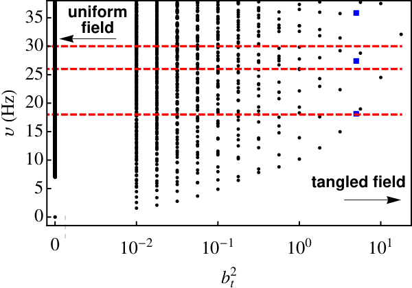
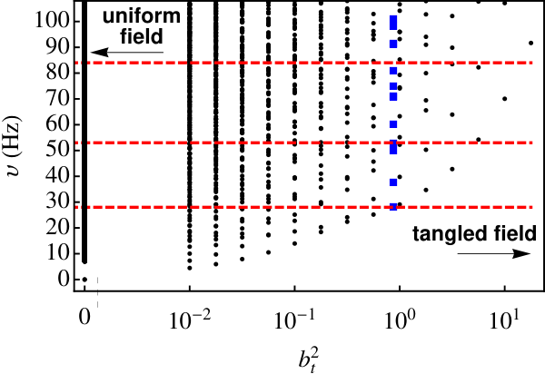
The splitting of the Alfvén continuum is shown in a different way in Figure 2, where realistic predictions are made for the eigenfrequencies in SGR 1806 (left) and 1900 (right). In contrast with Figure 1 where the total magnetic field was held constant ( G), we now fix the ordered field in each magnetar to its observed dipole spin-down value: G for SGR 1806 and G for SGR 1900. We take the fiducial values of , in each magnetar. Eigenfrequencies for all and for the range of frequencies shown are plotted. For , there exists an Alfvén continuum that begins at Hz, with a zero-frequency solution corresponding to rigid-body rotation. As is increased, the continuum splits into discrete normal modes. As is further increased and the modes spread out further, the higher-frequency modes move off the diagram. For large the eigenfrequencies become large due to the large tangled field.
The observed QPO frequencies in SGRs 1806 and 1900 are shown in Figure 2 as horizontal red dashed lines. For given and , the model has only as a free parameter, and gives quantitative predictions. Assuming the lowest observed QPO corresponds to the lowest eigenfrequency in the spectrum fixes the value of in each object, giving 5.0 and 0.87 for SGR 1806s and 1900 respectively. Eigenfrequencies for these are plotted as solid blue squares.
| 1 | 0 | 39 | 62 | 85 | 108 | 130 | 153 |
|---|---|---|---|---|---|---|---|
| 2 | 18 | 49 | 73 | 96 | 119 | 142 | |
| 3 | 27 | 58 | 81 | 104 | 126 | 148 | |
| 4 | 36 | 67 | 91 | 114 | 137 | 160 | |
| 5 | 44 | 76 | 100 | 123 | 145 | ||
| 6 | 52 | 84 | 109 | 133 | 155 | ||
| 7 | 59 | 93 | 118 | 142 |
| 1 | 0 | 52 | 89 | 126 | |
|---|---|---|---|---|---|
| 2 | 28 | 71 | 108 | 144 | |
| 3 | 38 | 75 | 109 | 145 | |
| 4 | 50 | 91 | 127 | ||
| 5 | 60 | 98 | 130 | ||
| 6 | 70 | 112 | 147 | ||
| 7 | 81 | 121 | 152 | ||
| 8 | 91 | 134 | |||
| 9 | 101 | 144 | |||
| 10 | 111 | 155 |
In Tables 2 and 3, we give frequencies for SGR 1806 and 1900 at and respectively. Numbers in boldface denote normal mode frequencies that are within 3 Hz of an observed QPO in both SGRs 1806 and 1900, and represent plausible mode identifications. Within these tolerances, every observed QPO frequency below 160 Hz in SGRs 1806 and 1900 is accounted for. For SGR 1806, the model does not give the distinct 26 Hz and 30 Hz that have been reported, but we note that these features are quite broad (Watts & Strohmayer, 2006). The reported frequencies have uncertainties, and drift with time, and analysis has not yet been done to determine if the data favor two frequencies around 26-30 Hz, or only one. In our model, both are accommodated by the 27 Hz frequency for this example. If distinct QPOs at 26 and 30 Hz could be ascertained, this would challenge our model.


Examples of eigenmodes are plotted in Figure 3. The left panel shows the 93 Hz mode of SGR 1806, with the attribution , , while the right panel shows the 155 Hz of SGR 1806, with the attribution , . The left panel has , which is close to the isotropic limit, and shows a large degree of spherical structure symmetry. In the plot on the right, , and the mode shows mostly cylindrical structure, a characteristic feature of the continuum.
Though our simple, constant density model is intended mostly for illustration, it accurately reproduces all observed QPOs in SGRs 1806 and 1900 though the spectrum is rather dense with a spacing of about 10 Hz. The main goal has been to show in a quantitative manner how the Alfvén continuum is broken. As we show in §6, the effects of realistic stellar structure are generally small (except for low- fundamentals), and so this constant-density model is sufficiently accurate for semi-quantitative study of torsional oscillations. Many of the predicted frequencies have not been observed, and we discuss this further below.
All examples shown here are for km. If is reduced, it is necessary to decrease to obtain similar fits to the data. The spectrum becomes generally less dense. Larger has the opposite effect.
6 Effects of stratification and the Crust
We now show that density stratification and crust rigidity gives corrections to the eigenfrequencies of the constant-density model considered thus far of typically %, but up to 50% for low- fundamentals. Because our best fits to the data for the constant-density model give for SGR 1806 and for SGR 1900, we ignore the organized field, and study the isotropic problem corresponding to a strong magnetic tangle.
We construct a relativistic star using the analytic representation of the Brussels-Montreal equation of state derived by Potekhin et al. (2013). For a 1.4 neutron star, we obtain a radius of 13.1 km. We take , and and fix the magnetic field at G. The shear modulus is from Strohmayer et al. (1991). For this spherical problem, the variable separation proceeds as in §4. We solve numerically for the radial eigenfunctions and eigenfrequencies. As a baseline for comparison, Table 1 can be scaled according to eq. (23) to obtain the eigenfrequencies for a constant-density star of radius 13.1 km. We assume that the dynamical density in the crust is equal to the total mass density, so that the entrainment of superfluid neutrons in the crust Chamel (2005); Chamel (2012) is effectively perfect. Entrainment, or lack of entrainment, has little effect on our results.
To explore the individual effects of stratification and the crust, we first examined a stratified star with no crust. We find that stratification lowers the frequencies for all modes with the exception of the modes, which are raised; typical changes are % for and -15% for . This general trend was also found by Passamonti & Lander (2014). The reason for the frequency decrease (except for ) can be seen by noting that the frequency scales as in the case of uniform density; see eq. (23). The stratified star has more mass concentrated in the central regions of the star, making it behave effectively as a smaller star compared to a constant-density star of the same radius.
Next, we considered a stratified star with a crust. The addition of a crust increases all frequencies by for and 1-5% for compared with the stratified case. The crust increases the frequency because it increases the average shear modulus of the star. The effect is small because the shear modulus of the crust exceeds in only a small fraction of the stellar volume. The effects of crust rigidity are therefore small compared to the rigidity introduced by the tangled field throughout the star, and the modes are unchanged to two significant figures. A simple analysis is given in Appendix B that further quantifies this effect. By contrast, the rigidity of the crust is essential an essential ingredient if the field is not significantly tangled, as considered in previous work (e.g., van Hoven & Levin 2011; Colaiuda & Kokkotas 2011; Gabler et al. 2011; Gabler et al. 2012; van Hoven & Levin 2012; Gabler et al. 2013a; Gabler et al. 2013b; Gabler et al. 2014).
| 1 | 0 | -15% | -15% | -16% | -15% | -16% | -16% |
|---|---|---|---|---|---|---|---|
| 2 | +48% | -8.9% | -12% | -14% | -15% | -15% | -15% |
| 3 | +41% | -4.5% | -10% | -12% | -13% | -14% | -14% |
| 4 | +35% | -1.9% | -8.0% | -11% | -12% | -13% | -14% |
| 5 | +31% | -0.47% | -6.5% | -9.4% | -11% | -12% | -13% |
| 6 | +27% | 0.33 % | -5.6% | -8.5% | -10% | -11% | -12% |
.
On the balance, stratification has a larger effect than does the crust. The combined effects of stratification and a crust is presented in Table 4, where the percentage change in frequencies compared with a constant density star of 13.1 km radius are given. For the modes, the combined effects of stratification and a crust increase frequencies by up to 50%, because both effects add. For the frequencies drop as a result of stratification, but are enhanced slightly by the crust giving a net change of up to 16%. Changes become more pronounced for increasing , but less pronounced for increasing .
We conclude that for star in which the tangled field accounts for much of the magnetic energy density (), that both density stratification and the crust rigidity have a relatively small effect on the frequencies of torsional normal modes. The constant-density model is an accurate first approximation at the 10% level for most overtones, and better than 50% for fundamental modes.
7 Energetics
The only quantitative discussion to date of the energetics of QPO excitation has been given by Levin & van Hoven (2011). We use the results of their analysis to calculate the mode amplitude at the stellar surface in the global oscillation interpretation of QPOs, and the total energy in the low-frequency QPOs.
The natural candidate for the energy source that excites stellar modes is the flare itself. For giant flares, the energy cannot be released deep inside the star, as the impedance mismatch between the stellar interior and the magnetosphere is so great that the energy in Alfvén waves would take seconds or longer to reach the magnetosphere due to multiple reflections, in conflict with observed rise times of ms (Link, 2014). This constraint favors an external origin for flares, as suggested by Lyutikov (2003); Lyutikov (2006), Komissarov et al. (2007), and Gill & Heyl (2010). Forcing of the magnetosphere through episodic release of internal magnetic energy could produce a magnetospheric explosion when an MHD instability is triggered.
Levin & van Hoven (2011) considered the excitation problem under the assumption that the magnetosphere undergoes a sudden change (over several relativistic Alfvén wave crossing times in the magnetosphere, s) from one equilibrium configuration to another, exciting torsional oscillations in the star. Suppose the shear stress at the surface changes by , where is the characteristic field strength in the inner magnetosphere, and . The average displacement at the stellar surface, assuming excitation of global mode with frequency , is of order (Levin & van Hoven 2011; eq. 11)
| (30) |
where erg is the characteristic magnetic energy available to be released; is the total energy released, and should be comparable to the flare energy. The scaling as follows from the Fourier transform of a step function.
The energy in a mode is of order (Levin & van Hoven 2011; eq. 12)
| (31) |
Most of the energy is in low-frequency modes. We have found a fairly dense spectrum with a characteristic mode spacing of Hz. The sum of the total energy in all modes can be approximated with an integral
| (32) |
where is the lowest-frequency normal mode in the spectrum. We see that the conversion of magnetospheric energy to mechanical motion in the star an inefficient process; about 0.1% of the flare energy goes into normal modes. The total energy in the modes in our model is well within the energy budget of a giant flare.
For a small flare, with erg, the amplitude from eq. 30 is smaller by than if is liberated. These estimates hold not just for our model, but generally for any global-oscillation model of QPOs.
8 Discussion and Conclusions
We propose a new physical scenario for magnetar oscillations wherein the Alfvén continuum supported by the organized field is broken by nearly isotropic stresses arising from components of the field that form a complex tangle over scales much smaller than the stellar radius. In a simple model of constant density, an organized field of strength G, and a tangled field of comparable strength, a fundamental frequency appears near 20 Hz for and , with a with a mode spacing of Hz (we use from the solutions of the isotropic problem to label the modes of the anisotropic problem). The model is consistent with QPOs observed in SGRs 1806 and 1900 below about 160 Hz. Magnetic stresses dominate material stresses almost everywhere in the crust, so crust elasticity is unimportant when a strong, tangled field is present. We find that the combined effects of realistic stellar structure and crust stress give a modest change in the eigenfrequencies of % for most modes (but up to 50% for low- fundamentals) so our simple model with constant density is a good first approximation to studying tangled fields that elucidates the essential physics. The strength of the organized field, which should be approximately dipolar, is determined observationally. Once stellar mass and radius are fixed, the model has only one important free parameter: the ratio of the energy densities in tangled and organized fields.
Our results are insensitive to whether or not the protons are superconducting. The upper critical field for type II superconductivity is G, comparable to average fields we find to be consistent with the QPOs observed in SGRs 1806 and 1900; the magnetic stress is nearly the same if the protons are superconducting, though we have assumed for definiteness that they are normal. Also, if the protons are superconducting, the neutrons are only slightly entrained by the protons throughout most of the core, and the dynamical mass density is nearly equal to the proton mass density in this case as well.
While our constant-density model is mostly illustrative, it is nevertheless sufficiently accurate to study torsional oscillations semi-quantitatively within our approximations; the model is able to account for every QPO observed in SGRs 1806 and 1900 to within 3 Hz. No other published model has given such quantitative agreement, though we acknowledge that the success of the model is due in large part to the rather dense spectrum we predict with a frequency spacing of about 10 Hz. We find the data are best explained if there is approximate equipartition of the energy in the smooth and tangled fields. Such modes have high enough wavenumbers to probe the field structure over scales below , at which point the averaging procedure we introduced to treat the tangled field might become inappropriate.
Why have most of the predicted frequencies not been observed? One possibility is that the modes have been excited, but are not visible. Given that we do not understand how surface oscillations affect magnetospheric emission, it could be that some modes are not seen because they do not produce sufficiently large changes in the x-ray emissivity to be visible from our viewing angle. Another possibility is that the instability that drives the flare creates highly-preferential excitation of axial modes. We note that preferential excitation of low-frequency free oscillations occurs in the Earth (Rhie & Romanowicz, 2004), the so-called “hum”. The question of how preferential excitation of stellar modes might occur is an interesting question.
While our focus has been on SGRs 1806 and 1900, which have dipole fields of G, QPOs have been reported for SGR J1550-5418 (Huppenkothen et al., 2014) in association with burst storms. SGR J1550-5418 has an inferred dipole field of G (Camilo et al., 2007). In this object, as in SGR 1900, the observed QPOs can be accounted for if most of the magnetic energy is in the tangled field, so that the average magnetic field is G.
A crucial ingredient in the interpretation of QPOs as stellar oscillations is to understand how crust movement can produce the large observed modulations of the x-ray emission by 10-20%. Timokhin et al. (2008) propose that twisting of the crust, associated with a stellar mode, modulates the charge density in the magnetosphere, creating variations in the optical depth for resonant Compton scattering of the hard x-rays that accompany the flare. In that model, the shear amplitude at the stellar surface must be as large as 1% of the stellar radius. D’Angelo & Watts (2012) accounted for geometrical effects of the beamed emission, and find that the amplitude of the QPO emission is increased by a factor of typically several over the estimate of Timokhin et al. (2008) for a given amplitude of the surface displacement. Based on the analysis of Levin & van Hoven (2011) of mode excitation by a sudden change in magnetospheric equilibrium, we find that the predicted, low-frequency QPO spectrum could contain up to erg in mechanical energy. This number is well within the energy budget of giant flares but the surface amplitude is only , smaller than required by Timokhin et al. (2008), especially for the QPOs near 160 Hz. This small amplitude could spell trouble for the global-oscillation interpretation of QPOs, unless a more efficient mechanism than that of Timokhin et al. (2008) can be identified. Explaining QPOs in small bursts ( erg) appears particularly difficult with a global oscillation model. The mode amplitude scales as the flare energy (eq. 30), giving a surface amplitude that is times smaller than for a giant flare. The 626 Hz QPO reported in SGR 1806 also seems problematic to excite in a giant flare, with a surface amplitude of in the most optimistic case. These numbers show that energetics should be given serious consideration in QPO models, and that other excitation mechanisms than that of Levin & van Hoven (2011) should be considered.
The simple model presented in this paper can be improved by including a crust and introducing realistic stellar structure. We have shown that the effects typically for most modes for a star in which the magnetic energy density is dominated by that in the tangled field; the effects of stellar structure and the crust will become more important as the effective shear modulus from the tangled field is reduced, and we have not quantified these effects. Other modes than axial modes, such as polar modes, should be considered as well.
An explanation for why the observed frequencies are quasi-periodic is well beyond the scope of our model. Quasi-periodicity could arise from magnetospheric effects, dynamics in the star not included here, or both.
Acknowledgments
We thank M. Gabler, D. Huppenkothen, Y. Levin, and A. Watts for very helpful discussions, and Y. Levin and A. Watts for comments on the manuscript. This work was supported by NSF Award AST-1211391 and NASA Award NNX12AF88G.
Appendix A Variable Separation
Eqs. (25) and (26) can be separated and solved by transforming to an oblate spheroidal coordinate system defined by
| (33) |
| (34) |
Curves of constant are ellipses, and curves of constant are hyperbolae. For , the coordinate gives a sphere of radius . In the limit , spherical coordinates are recovered with and .
The boundary condition eq. (26) at becomes
| (36) |
while at we require
| (37) |
for odd parity modes or
| (38) |
for even parity modes.
We seek a separable solution of the form
| (39) |
Eq. (A) becomes
| (40) |
| (41) |
where is the separation constant. The boundary condition eq. (36) becomes
| (42) |
at . The boundary conditions (37) and (38) are satisfied if we impose
| (43) |
for odd parity modes or
| (44) |
for even parity modes.
In the limit , eq. (40) reduces to the spherical Bessel equation with solution , while (41) reduces to an associated Legendre equation with solution and , which recovers the solutions of the isotropic model of §4.
For arbitrary the modes are identified by the number of nodes; for the mode the function has nodes on the domain , while for the mode the function has nodes on .
Appendix B Effects of the Crust
The comparisons to observed QPOs in §5 suggest , so that erg cm-3. The shear modulus crust exceeds this value only in the densest regions of the crust. The rigidity of the crust will increase the normal-mode frequencies somewhat with respect to what we have found by neglecting the crust. Here we show that crust rigidity has small or negligible effects on our results.
To estimate the effect, we consider a two-component isotropic model with only a tangled field. The core liquid, which we take to be homogeneous, has an effective shear modulus and a shear-wave speed . The crust, which we also take to be homogeneous, has shear modulus and a shear-wave speed . The crust has an inner radius and outer radius .
In the core, the solution to the mode problem is ; the mode frequency is . The solution in the crust is , where are spherical Neumann functions, and are constants, and . The boundary conditions are continuity in value and traction at , and vanishing traction at :
| (45) |
| (46) |
| (47) |
The shear modulus in the crust, ignoring magnetic effects, is (Strohmayer et al., 1991)
| (48) |
where is the number density of ions of charge , is the Wigner-Seitz cell radius given by , and where is Boltzmann’s constant. Typically in the crust, and the second term in the denominator is negligible. For the composition of the inner crust, we use the results of Douchin & Haensel (2001), conveniently expressed analytically by Haensel & Potekhin (2004). We solve for crust structure using the Newtonian equation for hydrostatic equilibrium, for a stellar radius of 10 km and a stellar mass of 1.4 . In the evaluation of the shear-wave speed in the crust, we include the effects of nuclear entrainment (Chamel, 2005; Chamel, 2012). Further details are given in Link (2014).
We find that drops from erg cm-3 at the base of the crust to erg cm-3 over 370 m. Because we have assumed a homogeneous crust, we take the geometric mean of over this range, which is erg cm-3, and set the crust thickness to 370 m. (The matter in the remainder of the crust contributes less to the rigidity than does the tangled field). The shear speed in the crust varies by a factor of about two in this region, with a geometric mean of . With these values, we solve the boundary conditions numerically for the corrected eigenfrequencies. Crust rigidity increases the mode frequency by % for each fundamental of a given , and % for harmonics.
The treatment by Douchin & Haensel (2001) of the inner crust gives somewhat higher values of the shear modulus at the base of the crust than do other studies. The equation of state of Akmal et al. (1998), for example, gives a shear speed at the base of the crust that is about 0.6 the shear speed of Douchin & Haensel (2001), and a corresponding shear modulus that is smaller by a factor of about 2.8. Reducing the crust shear modulus by a factor of two, and repeating the above analysis, shows that crust rigidity increases the fundamental frequency for each by less than 10%.
References
- Akmal et al. (1998) Akmal A., Pandharipande V., Ravenhall D., 1998, Physical Review C, 58, 1804
- Barat et al. (1979) Barat C., Chambon G., Hurley K., Niel M., Vedrenne G., Estulin I., Kurt V., Zenchenko V., 1979, Astronomy and Astrophysics, 79, L24
- Camilo et al. (2007) Camilo F., Ransom S., Halpern J., Reynolds J., 2007, The Astrophysical Journal Letters, 666, L93
- Cerdá-Durán et al. (2009) Cerdá-Durán P., Stergioulas N., Font J. A., 2009, Mon. Not. Roy. Astron. Soc., 397, 1607
- Cerdá-Durán et al. (2009) Cerdá-Durán P., Stergioulas N., Font J. A., 2009, Monthly Notices of the Royal Astronomical Society, 397, 1607
- Chamel (2005) Chamel N., 2005, Nucl. Phys. A, 747, 109
- Chamel (2012) Chamel N., 2012, Phys. Rev. C, 85, 035801
- Chamel & Haensel (2006) Chamel N., Haensel P., 2006, Phys. Rev. C, 73, 045802
- Cline et al. (1980) Cline T., Desai U., Pizzichini G., Teegarden B., Evans W., Klebesadel R., Laros J., Hurley K., Niel M., Vedrenne G., 1980, The Astrophysical Journal, 237, L1
- Colaiuda et al. (2009) Colaiuda A., Beyer H., Kokkotas K., 2009, Monthly Notices of the Royal Astronomical Society, 396, 1441
- Colaiuda & Kokkotas (2012) Colaiuda A., Kokkotas K., 2012, Monthly Notices of the Royal Astronomical Society, 423, 811
- Colaiuda & Kokkotas (2011) Colaiuda A., Kokkotas K. D., 2011, Mon. Not. Roy. Astron. Soc., 414, 3014
- D’Angelo & Watts (2012) D’Angelo C., Watts A., 2012, The Astrophysical Journal Letters, 751, L41
- Douchin & Haensel (2001) Douchin F., Haensel P., 2001, Astron. Astrophys., 380, 151
- Duncan (1998) Duncan R. C., 1998, Astrophysics J., 489, L45
- El-Mezeini & Ibrahim (2010) El-Mezeini A. M., Ibrahim A. I., 2010, Astrophys. J. Lett., 721, L121
- Fenimore et al. (1996) Fenimore E. E., Klebesadel R. W., Laros J. G., 1996, Astrophys. J., 460, 964
- Feroci et al. (1999) Feroci M., Frontera F., Costa E., Amati L., Tavani M., Rapisarda M., Orlandini M., 1999, The Astrophysical Journal Letters, 515, L9
- Gabler et al. (2013a) Gabler M., Cerdá-Durán P., Font J. A., Müller E., Stergioulas N., 2013a, Monthly Notices of the Royal Astronomical Society, 430, 1811
- Gabler et al. (2012) Gabler M., Cerdá-Durán P., Stergioulas N., Font J. A., Müller E., 2012, Monthly Notices of the Royal Astronomical Society, 421, 2054
- Gabler et al. (2013b) Gabler M., Cerdá-Durán P., Stergioulas N., Font J. A., Müller E., 2013b, Physical review letters, 111, 211102
- Gabler et al. (2014) Gabler M., Cerdá-Durán P., Stergioulas N., Font J. A., Müller E., 2014, Monthly Notices of the Royal Astronomical Society, 443, 1416
- Gabler et al. (2011) Gabler M., Cerdaá-Durán P., Font J. A., Müller E., Stergioulas N., 2011, Mon. Not. Roy. Astron. Soc., 410, L37
- Gill & Heyl (2010) Gill R., Heyl J. S., 2010, Monthly Notices of the Royal Astronomical Society, 407, 1926
- Glampedakis et al. (2006) Glampedakis K., Samuelsson L., Andersson N., 2006, Mon. Not. Roy. Astron. Soc., 371, L74
- Goedbleod & Poedts (2004) Goedbleod J. P. H., Poedts S., 2004, Principles of Magnetohydrodynamics. Cambridge Univ. Press, Cambridge
- Haensel & Potekhin (2004) Haensel P., Potekhin A. Y., 2004, Astron. Astrophys., 428, 191
- Hambaryan et al. (2011) Hambaryan V., Neuhäuser R., Kokkotas K. D., 2011, Astron. Astrophys., 528, 45
- Huppenkothen et al. (2014) Huppenkothen D., D’Angelo C., Watts A. L., Heil L., van der Klis M., van der Horst A. J., Kouveliotou C., Baring M. G., Göğüş E., Granot J., et al., 2014, The Astrophysical Journal, 787, 128
- Huppenkothen et al. (2014) Huppenkothen D., Heil L., Watts A., Göğüş E., 2014, The Astrophysical Journal, 795, 114
- Huppenkothen et al. (2013) Huppenkothen D., Watts A. L., Uttley P., van der Horst A. J., van der Klis M., Kouveliotou C., Göğüş E., Granot J., Vaughan S., Finger M. H., 2013, The Astrophysical Journal, 768, 87
- Hurley et al. (1999) Hurley K., Cline T., Mazets E., Barthelmy S., Butterworth P., Marshall F., Palmer D., Aptekar R., Golenetskii S., Il’Inskii V., et al., 1999, Nature, 397, 41
- Israel et al. (2005) Israel G., Belloni T., Stella L., Rephaeli Y., Gruber D., Casella P., Dall’Osso S., Rea N., Persic M., Rothschild R., 2005, The Astrophysical Journal Letters, 628, L53
- Komissarov et al. (2007) Komissarov S., Barkov M., Lyutikov M., 2007, Monthly Notices of the Royal Astronomical Society, 374, 415
- Lee (2007) Lee U., 2007, Mon. Not. Roy. Astron. Soc., 374, 1015
- Levin (2006) Levin Y., 2006, Mon. Not. Roy. Astron. Soc., 368, L35
- Levin (2007) Levin Y., 2007, Mon. Not. Roy. Astron. Soc., 377, 159
- Levin & van Hoven (2011) Levin Y., van Hoven M., 2011, Monthly Notices of the Royal Astronomical Society, 418, 659
- Link (2014) Link B., 2014, Monthly Notices of the Royal Astronomical Society, 441, 2676
- Lyutikov (2003) Lyutikov M., 2003, Mon. Not. Roy. Astron. Soc., 346, 540
- Lyutikov (2006) Lyutikov M., 2006, Monthly Notices of the Royal Astronomical Society, 367, 1594
- Mazets et al. (1979) Mazets E., Golenetskii S., Il’Inskii V., Aptekar R., Guryan Y. A., 1979, Nature, 282, 587
- Mereghetti et al. (2006) Mereghetti S., Esposito P., Tiengo A., Zane S., Turolla R., Stella L., Israel G., Götz D., Feroci M., 2006, The Astrophysical Journal, 653, 1423
- Nakagawa et al. (2008) Nakagawa Y. E., Mihara T., Yoshida A., Yamaoka K., Sugita S., Murakami T., Yonetoku D., Suzuki M., Nakajima M., Tashiro M., et al., 2008, PASJ, 61, S387
- Passamonti & Lander (2013) Passamonti A., Lander S., 2013, Monthly Notices of the Royal Astronomical Society, 429, 767
- Passamonti & Lander (2014) Passamonti A., Lander S. K., 2014, MNRAS, 438, 156
- Piro (2005) Piro A. L., 2005, Astrophys. J., 634, L153
- Potekhin et al. (2013) Potekhin A., Fantina A., Chamel N., Pearson J., Goriely S., 2013, Astronomy & astrophysics, 560, A48
- Rhie & Romanowicz (2004) Rhie J., Romanowicz B., 2004, Nature, 431, 552
- Samuelsson & Andersson (2007) Samuelsson L., Andersson N., 2007, Mon. Not. Roy. Astron. Soc., 374, 256
- Sotani et al. (2007) Sotani H., Colaiuda A., Kokkotas K. D., 2007, Mon. Not. Roy. Astron. Soc., 385, 2162
- Sotani et al. (2007) Sotani H., Kokkotas K. D., Stergioulas N., 2007, Mon. Not. Roy. Astron. Soc., 375, 261
- Sotani et al. (2008) Sotani H., Kokkotas K. D., Stergioulas N., 2008, Mon. Not. Roy. Astron. Soc., 385, L5
- Steiner & Watts (2009) Steiner A. W., Watts A. L., 2009, Phys. Rev. Lett., 103, 181101
- Strohmayer et al. (1991) Strohmayer T. E., van Horn H. M., Ogata S., Iyetomi H., Ichimaru S., 1991, Astrophys. J., 375, 679
- Strohmayer & Watts (2005) Strohmayer T. E., Watts A. L., 2005, Astrophys. J., 632, L111
- Strohmayer & Watts (2006) Strohmayer T. E., Watts A. L., 2006, The Astrophysical Journal, 653, 593
- Tiengo et al. (2009) Tiengo A., Esposito P., Mereghetti S., Israel G., Stella L., Turolla R., Zane S., Rea N., Götz D., Feroci M., 2009, Mon. Not. Roy. Astron. Soc., 399, L74
- Timokhin et al. (2008) Timokhin A., Eichler D., Lyubarsky Y., 2008, The Astrophysical Journal, 680, 1398
- van Hoven & Levin (2011) van Hoven M., Levin Y., 2011, Mon. Not. Roy. Astron. Soc., 420, 1036
- van Hoven & Levin (2012) van Hoven M., Levin Y., 2012, Monthly Notices of the Royal Astronomical Society, 420, 3035
- Watts & Reddy (2007) Watts A. L., Reddy S., 2007, Mon. Not. Roy. Astron. Soc., 379, 63
- Watts & Strohmayer (2006) Watts A. L., Strohmayer T. E., 2006, Astrophys. J., 637, L117