Complementarity of LHC and EDMs for Exploring Higgs CP Violation

The most general two Higgs doublet potential which breaks $SU(2)_{L}\times U(1)$ to $U(1)_{EM}$ is,

The potential of Eq. (1) leads to tree level flavor changing neutral currents, which can be avoided by imposing a $Z_{2}$ symmetry under which,

Eq. (2) implies $\lambda_{6}=\lambda_{7}=0$, while a non-zero $m_{12}$ softly breaks the $Z_{2}$ symmetry of Eq. (2).

After electroweak symmetry breaking, the Higgs doublets in unitary gauge can be written as,

where $\tan\beta=v_{2}/v_{1}$, $v=\sqrt{\mid v_{1}\mid^{2}+\mid v_{2}\mid^{2}}=246$ GeV and $H^{+}$ is the physical charged Higgs with mass $m_{H^{+}}$. We are free to redefine fields and go to a basis where $\xi=0$. In general there are $2$ independent phases and the imaginary parts of $m_{12}$ and $\lambda_{5}$ lead to mixing in the neutral Higgs sector between $H_{1}^{0},H_{2}^{0}$ and $A^{0}$, and that is the source of CP violation.

The mixing among the three neutral scalars can be parametrized by an orthogonal matrix $R$,

where $s_{\alpha}=\sin\alpha$, etc and

The physical mass eigenstates are then defined as $(h_{1},h_{2},h_{3})^{T}=R(H_{1}^{0},H_{2}^{0},A^{0})^{T}$. In the CP conserving version of the 2HDM, $\alpha_{b}=\alpha_{c}=0$, $R$ is block diagonal, and $h_{1}$ and $h_{2}$ have no pseudoscalar component.

For simplicity, we focus on the 2HDMs where the Yukawa sector has a $Z_{2}$ symmetry and $\phi_{1}$ and $\phi_{2}$ each only gives mass to up or down type fermions. This is sufficient to suppress tree-level flavor changing processes mediated by the neutral Higgs scalars. For the $3rd$ generation (and suppressing CKM mixing),

where $Q_{L}^{T}=(t_{L},b_{L})$. In both cases, we assume that the charged lepton Yukawa coupling has the same form as that of the charge $-1/3$ quarks. Under the $Z_{2}$ symmetry, $Q_{L},t_{R},\phi_{2}$ are always even, $\phi_{1}$ is always odd, and $b_{R}$ is even (odd) in Type I (II) models.

From this we can derive the couplings between neutral Higgs bosons and the fermions and gauge bosons. As a general parametrization we take,

When $c_{f,i}\tilde{c}_{f,i}\neq 0$ or $a_{i}\tilde{c}_{f,i}\neq 0$, the mass eigenstate $h_{i}$ couples to both CP even and CP odd operators, so the theory violates CP. The coefficients $c_{f,i}$, $\tilde{c}_{f,i}$ and $a_{i}$ can be derived from $\tan\beta$ and the elements of the matrix $R$ defined above.

An appealing feature is that all couplings in Table 1 depend on only four parameters, $\alpha$, $\alpha_{b}$, $\alpha_{c}$ and $\tan\beta$. It is worth noting that the couplings of the light Higgs boson $h_{1}$ to the gauge bosons and fermions are independent of $\alpha_{c}$. Fits to the CP conserving 2HDM suggest that the couplings are close to the alignment limit, $\beta-\alpha\sim{\pi\over 2}$, implying that $h_{1}$ has couplings very close to the SM predictions. In our numerical studies, we will allow small deviations from the alignment limit.

In general, the imposed $Z_{2}$ symmetry in the Yukawa sector is not preserved by renormalization. The hard breaking $\lambda_{6},\lambda_{7}$ terms from the Higgs potential will induce couplings of $\phi_{1}$, $\phi_{2}$ to both up and down type quarks. This does not reintroduce any tree level flavor changing effects because the induced Yukawa matrices are still aligned with the corresponding fermion mass matrices. Motivated by this, a convenient choice is to forbid the $\lambda_{6},\lambda_{7}$ terms. In this case, the model has an approximate $Z_{2}$ symmetry, which is only softly broken by the $m_{12}^{2}$ term.

For the approximate $Z_{2}$ symmetric model, all of the potential parameters can be solved for in terms of the following parameters:

• •

  The scalar masses, $m_{h_{1}}$, $m_{h_{2}}$, $m_{h_{3}}$ and $m_{H^{\pm}}$

• •

  The neutral scalar mixing angles, $\alpha$, $\alpha_{b}$, $\alpha_{c}$

• •

  The ratio of vev’s, $\tan\beta$

• •

  One potential parameter, ${\rm Re}(m_{12}^{2})$, or $\nu\equiv{\rm Re}(m_{12})^{2}/({{v^{2}\sin 2\beta}})$  ,

giving $9$ physical parameters. The $\nu$ parameter controls the decoupling limit, i.e., when ${\rm Re}(m_{12})^{2}$ approaches infinity, the masses of $h_{2}$, $h_{3}$ and $H^{\pm}$ also go to infinity.

The explicit solution for the parameters of the scalar potential was found in Ref. [10], and is listed below in Appendix A. The imaginary part of $\lambda_{5}$, which is a source of CP violation, is given by,

An important point here is that, in order for the 126 GeV Higgs boson to have CP violating couplings, the heavy Higgs states must not decouple. Otherwise, the two Higgs doublet model will return to the SM limit. This is actually our main motivation for studying the bounds on the non-decoupled heavy Higgs.

Clearly, when the scalars $h_{2,3}$ are much heavier than the electroweak scale, and $m_{h_{2}}\simeq m_{h_{3}}\equiv m_{H^{+}}\gg m_{h_{1}}$,

The unitarity bound on ${\rm Im}\lambda_{5}$, ${\rm Im}\lambda_{5}<4\pi$, sets the largest allowed CP violating mixing angle $\alpha_{b}$. This implies that for an ${\cal{O}}(1)~\sin\alpha_{b}$ to be theoretically accessible, the heavy scalars $h_{2}$, $h_{3}$ and $H^{\pm}$ must be not far above the electroweak scale. In general, for nonzero $\alpha_{b}$, the masses of the heavy scalars should satisfy

A similar conclusion holds when one goes beyond the approximate $Z_{2}$ symmetry by including the $\lambda_{6},\lambda_{7}$ terms.

For the approximate $Z_{2}$ symmetric model, there is a further theoretical constraint on the physical parameters resulting from the minimization of the potential. This constraint is given in Eq. (A) and can be transformed into a quadratic equation for $\tan\alpha_{c}$. The condition for $\alpha_{c}$ to have a real solution is

When Eq. (13) is satisfied, the solutions for $\alpha_{c}$ are,

Eq. (13) implies an additional theoretical upper bound on the CP violating angle $\alpha_{b}$, when the other parameters are fixed. In practice, we sometimes find this bound can be stronger than all the experimental limits. However, this is only a bound because of theoretical prejudice. In fact, it can be removed with a minimal step beyond the approximate $Z_{2}$ symmetric case by introducing a $\lambda_{7}$ term, with $\lambda_{7}$ being purely imaginary. In this case, the bound Eq. (13) no longer exists, $\alpha_{c}$ becomes a free parameter, and ${\rm Im}\lambda_{7}$ can in turn be solved for as,

Although introducing hard $Z_{2}$ breaking ($\lambda_{6,7}\neq 0$) makes the Yukawa structure in Eq. (2.2) unnatural, one might argue it is accidentally the case at the electroweak scale. ¹¹ 1 We are aware that allowing $Z_{2}$ breaking terms in the Yukawa sector can introduce additional sources of CP violation. The price for this is introducing tree level flavor changing effects at the same time, and some flavor alignment mechanism must be resorted to [39, 40, 41]. We do not consider such a possibility, but focus on CP violation only from the Higgs sector in this work. In the phenomenological study in the next section, we will give the results for both the approximate $Z_{2}$ case, and the minimal extension as discussed in this subsection.

At this point, it is useful to gain some intuition about the impact of CP violation on the heavy Higgs to gauge boson decay channels, $h_{i}\to VV$ and $h_{i}\to Zh_{1}$ with $(i=2,3)$. It is convenient to redefine the Higgs doublets and go to a basis where only one doublet, called $\phi_{1}^{\prime}$, gets the 246 GeV vev, while the other $\phi_{2}^{\prime}$ has no vev [67, 13].

We start from a special point in the parameter space where the lightest Higgs, $h_{1}$, has exactly the same couplings does the SM Higgs boson. This corresponds to having the mixing angles in Eq. (4) satisfy $\alpha_{b}=\alpha_{c}=0$, and $\beta-\alpha=\pi/2$. The Higgs sector preserves CP invariance at this point. In this case, $h_{1}$ is the excitation arising from $\phi_{1}^{\prime}$ defined above, while $h_{2,3}$ are excitations from $\phi_{2}^{\prime}$. As a result, the decay rates $h_{i}\to VV$ and $h_{i}\to Zh_{1}$ both vanish for $i=2,3$. It is worth noticing that this special point can be approached without going to the real decoupling limit by sending the second doublet mass to infinity.

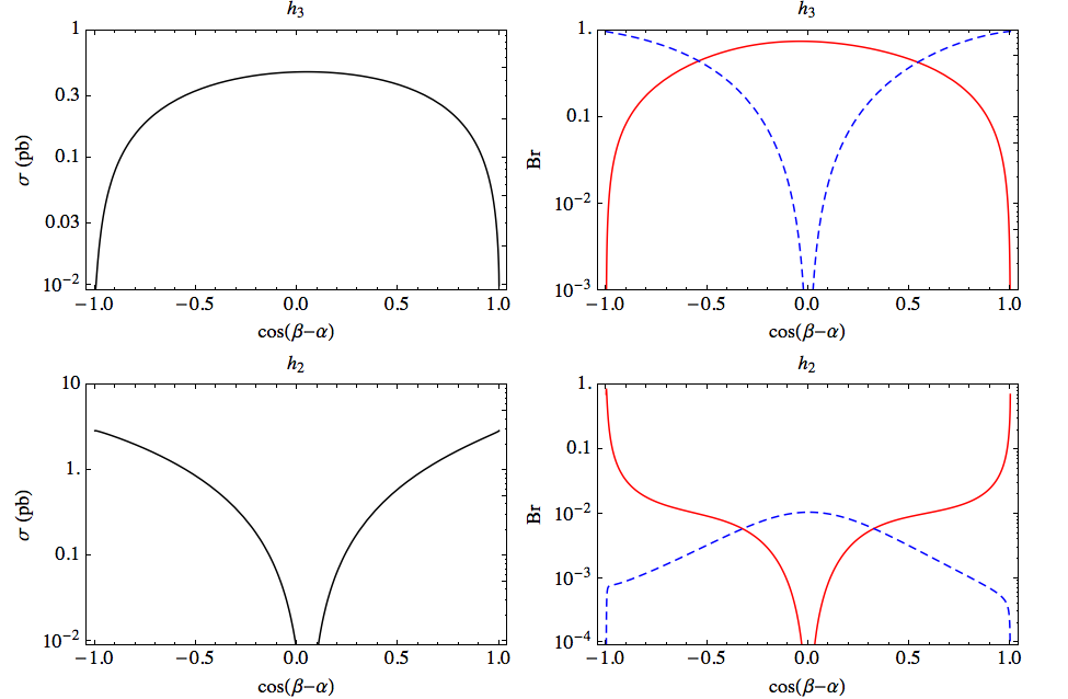
Next, we turn on CP violation by making $\alpha_{b}=0.5$, but still keep $\alpha_{c}=0$. Here we discuss an example by fixing $\tan\beta=20$ (in the basis of $\{\phi_{1},\phi_{2}\}$ given in Eq. (3)) and vary the angle $\alpha$, or the quantity $\cos(\beta-\alpha)$. We also choose the heavy neutral scalar masses to be $m_{h_{2}}=400\,$GeV and $m_{h_{3}}=450\,$GeV. In Fig. 1, we plot the gluon fusion production cross section and the gauge boson branching ratios of $h_{2,3}$ as a function of $\cos(\beta-\alpha)$. There are several suppressed regions which can be understood from Table 1. In the case $\alpha_{c}=0$, we have in the Type-I model,

First, the gluon fusion production cross section for $h_{2}$ via a top or bottom loop vanishes at $\alpha=0$ (near $\cos(\beta-\alpha)\simeq 0$). In the example we describe here, $\beta=\arctan(20)$ is close to $\pi/2$, and $c_{t,2}=c_{b,2}$ vanishes at $\alpha=0$. Second, at $\alpha=\pm\pi/2$, (near $\cos(\beta-\alpha)\simeq\pm 1$), the couplings $c_{t,3}$ and $c_{b,3}$ vanish. As a result, the production cross section for $h_{3}$ is suppressed because $\tilde{c}_{t,3}$ and $\tilde{c}_{b,3}$ are both suppressed by $\cot\beta=1/20$ in this case.

On the other hand, the gauge boson decays of $h_{2,3}$ are directly controlled by $\beta-\alpha$. We list the relevant couplings here, again for $\alpha_{c}=0$,

where $g_{iz1}\ (i=2,3)$ is the coupling between $h_{i}$-$Z$-$h_{1}$ defined below Eq. (30). These make it manifest why the heavy Higgs to gauge boson decay channels are sensitive both to a deviation from the alignment limit and to CP violation. Clearly, when $\cos(\beta-\alpha)=\pm 1$, the decay rates $h_{3}\to VV$ and $h_{2}\to Zh_{1}$ vanish, while when $\cos(\beta-\alpha)=0$, the decay rates $h_{2}\to VV$ and $h_{3}\to Zh_{1}$ vanish. For the case of $h_{2}$ decay, the branching ratios are more suppressed because the decay $h_{2}\to h_{1}h_{1}$ dominates in most of the parameter space. Therefore, the most important constraints come from the $h_{3}\to VV$ and $h_{3}\to Zh_{1}$ channels.

Combining Eqs. (35) and (36), we find the $h_{3}\to VV$ signal rate (production cross section $\times$ decay branching ratio) is peaked at $\cos(\beta-\alpha)=0$, while $h_{3}\to Zh_{1}$ vanishes at both $\cos(\beta-\alpha)=0,\pm 1$, and is peaked in between. With these facts, one can understand the yellow and orange regions in the upper right panel of Fig. 11. One can also follow a similar analysis in order to understand the generic features in the other plots.

We first discuss the models with an approximate $Z_{2}$ symmetry. Fig. 3 shows the limits on the CP violating parameter, $\alpha_{b}$, as a function of $\tan\beta$ in the Type-I model. In each panel, the gray area marked “theory inaccessible” has no real solution for $\alpha_{c}$ from Eq. (2.4). The left panel assumes the alignment limit, $\beta-\alpha\sim{\pi/2}$, while the right panel allows for a small deviation from the alignment limit⁴⁴ 4 The results are similar for negative $\Delta$.. The orange area is excluded by the heavy Higgs search channel $h_{2,3}\rightarrow Zh_{1}\rightarrow l^{+}l^{-}b{\overline{b}}$, while the yellow area is excluded by the channel $h_{2,3}\rightarrow WW/ZZ$. It is clear that the limits become quite stringent away from the alignment limit. For comparison, we include the results of Ref. [10] for the limits from the electron EDM (eEDM, the blue shaded regions are excluded). In all cases, the EDM limit and the heavy Higgs searches exclude complementary regions. The masses of the heavy Higgs are increased to around 600 GeV in Fig. 4. In this case, the limits from heavy Higgs searches become much weaker, with the dominant excluded region coming from the eEDM searches. The mass splitting between the heavy masses is restricted by limits on the oblique parameters, which is discussed in Sec. 4.1.

Fig. 5 shows the limits on $\alpha_{b}$ versus $\tan\beta$ in the Type-II model. Away from the alignment limit (the right panel), there is a significant exclusion region for $\tan\beta\gtrsim 10$ from the $126$ GeV Higgs parameter measurements. Around $\tan\beta\sim 1$, the electron EDM constraint vanishes due to a cancellation among the Barr-Zee diagrams as pointed out in Ref. [8]. We find the heavy Higgs searches from the gauge boson decay channels $h_{2,3}\rightarrow Zh_{1}$ and $h_{2,3}\rightarrow WW/ZZ$ are extremely useful and close the window of large values of $\sin\alpha_{b}\sim\mathcal{O}(1)$ in all cases. As the mass of the heavy particles is increased in Fig. 6, the region excluded by the heavy Higgs searches shrinks, with again the dominant exclusion coming from the eEDM and neutron EDM (nEDM, the green regions are excluded). It is worth pointing out that the neutron EDM excluded regions are shown using the central values given in [60], which however involves large uncertainties in the evaluation of hadronic matrix elements. In contrast, the heavy Higgs searches provide a robust upper limit on the CP violating angle $\alpha_{b}$.

As discussed in Sec. 2.4, if the assumption of an approximate $Z_{2}$ symmetry is relaxed, the theoretical relationship between $\alpha_{b}$ and $\alpha_{c}$ can be removed. In this case $\alpha_{c}$ becomes a free parameter. This helps to remove the theoretically inaccessible region in Figs. 3–6, and one can get a complete view of various constraints in the whole parameter space.

Figs. 7 and 8 show the constraints in the Type-I model with $\alpha_{c}$ chosen equal to 0 or $\alpha_{b}$, and with two sets of heavy Higgs masses. It is apparent that the dependence on $\alpha_{c}$ is rather weak. The results in the Type-II model are shown in Figs. 9 and 10. In Figs. 11 and 12, the heavy Higgs search constraints are also displayed in the $\alpha_{b}$ and $\cos(\beta-\alpha)$ plane.

It is also worth re-emphasizing that at low $\tan\beta\sim\mathcal{O}(1)$ the 126 GeV Higgs data puts a very weak constraint on the CP violating angle $\alpha_{b}$. This can also be understood from Table 1, where the lightest (126 GeV) Higgs couplings to other SM particles near the alignment limit are

where $\Delta=\cos(\beta-\alpha)$ and we have kept terms up to first power in $\Delta$. Clearly for small $\Delta$ and $\tan\beta\approx 1$, all CP even couplings are approximately $\cos\alpha_{b}$ and all CP odd couplings $\approx\pm\sin\alpha_{b}$. They approach the values in the SM limit when $\alpha_{b}\to 0$. In the presence of CP violation, the gluon fusion production cross section of the light Higgs gets rescaled from the SM value by a factor [8, 10], $\sigma(gg\to h_{1})/\sigma_{\rm SM}(gg\to H_{SM})\simeq 1+1.42\sin^{2}\alpha_{b}$. The vector boson fusion and associated production rates get suppressed by $\sigma(VV\to h_{1})/\sigma_{\rm SM}(VV\to H_{SM})=\cos^{2}\alpha_{b}$. The light Higgs to fermion ($h_{1}\to b\bar{b},\tau^{+}\tau^{-}$) decay rates are not affected because the CP even and CP odd couplings contribute incoherently, $\Gamma(h_{1}\to f\bar{f})/\Gamma_{\rm SM}(h\to f\bar{f})=\cos^{2}\alpha_{b}+\sin^{2}\alpha_{b}=1$. The Higgs to gauge boson ($h_{1}\to WW^{*},ZZ^{*}$) decay rates get suppressed, $\Gamma(h_{1}\to VV^{*})/\Gamma_{\rm SM}(h_{1}\to VV^{*})=\cos^{2}\alpha_{b}$. The light Higgs to diphoton decay rate in the presence of CP violation has been given in refs. [8, 10], which in this case can be simplified to $\Gamma(h_{1}\to\gamma\gamma)/\Gamma_{\rm SM}(h\to\gamma\gamma)\simeq 1-0.81\sin^{2}\alpha_{b}$. As a result, the final $\chi^{2}$ of the fit for the 126 GeV Higgs data depends on $\cos^{2}\alpha_{b}$, and for the SM case $\chi^{2}_{\rm SM}=\chi^{2}(\cos^{2}\alpha_{b}\to 1)$. Because the $\cos^{2}\alpha_{b}$ function is very flat near $\alpha_{b}=0$, one can maintain a fit as good as in the SM for sizable $\alpha_{b}$.

References

• (1) G. Aad et al. [ATLAS Collaboration], Phys. Lett. B 716, 1 (2012) [arXiv:1207.7214 [hep-ex]].
• (2) S. Chatrchyan et al. [CMS Collaboration], Phys. Lett. B 716, 30 (2012) [arXiv:1207.7235 [hep-ex]].
• (3) G. C. Branco, P. M. Ferreira, L. Lavoura, M. N. Rebelo, M. Sher and J. P. Silva, Phys. Rept. 516, 1 (2012) [arXiv:1106.0034 [hep-ph]].
• (4) The ATLAS collaboration, ATLAS-CONF-2014-010, ATLAS-COM-CONF-2014-011.
• (5) C. Y. Chen and S. Dawson, Phys. Rev. D 87, 055016 (2013) [arXiv:1301.0309 [hep-ph]].
• (6) B. Coleppa, F. Kling and S. Su, JHEP 1401, 161 (2014) [arXiv:1305.0002 [hep-ph]].
• (7) K. Cheung, J. S. Lee and P. Y. Tseng, JHEP 1401, 085 (2014) [arXiv:1310.3937 [hep-ph]].
• (8) J. Shu and Y. Zhang, Phys. Rev. Lett. 111, no. 9, 091801 (2013) [arXiv:1304.0773 [hep-ph]].
• (9) D. E. Morrissey and M. J. Ramsey-Musolf, New J. Phys. 14, 125003 (2012) [arXiv:1206.2942 [hep-ph]].
• (10) S. Inoue, M. J. Ramsey-Musolf and Y. Zhang, Phys. Rev. D 89 (2014) 11, 115023 [arXiv:1403.4257 [hep-ph]].
• (11) J. Brod, U. Haisch and J. Zupan, JHEP 1311, 180 (2013) [arXiv:1310.1385 [hep-ph], arXiv:1310.1385].
• (12) D. Fontes, J. C. Rom‹o, R. Santos and J. P. Silva, arXiv:1502.01720 [hep-ph].
• (13) L. Lavoura and J. P. Silva, Phys. Rev. D 50, 4619 (1994) [hep-ph/9404276].
• (14) A. Barroso, P. M. Ferreira, R. Santos and J. P. Silva, Phys. Rev. D 86, 015022 (2012) [arXiv:1205.4247 [hep-ph]].
• (15) V. Khachatryan et al. [CMS Collaboration], arXiv:1411.3441 [hep-ex].
• (16) The ATLAS Collaboration, ATLAS-CONF-2013-013.
• (17) R. Harnik, A. Martin, T. Okui, R. Primulando and F. Yu, Phys. Rev. D 88, no. 7, 076009 (2013) [arXiv:1308.1094 [hep-ph]].
• (18) F. Bishara, Y. Grossman, R. Harnik, D. J. Robinson, J. Shu and J. Zupan, JHEP 1404, 084 (2014) [arXiv:1312.2955 [hep-ph]].
• (19) Y. Chen, A. Falkowski, I. Low and R. Vega-Morales, Phys. Rev. D 90, 113006 (2014) [arXiv:1405.6723 [hep-ph]].
• (20) M. J. Dolan, P. Harris, M. Jankowiak and M. Spannowsky, Phys. Rev. D 90, no. 7, 073008 (2014) [arXiv:1406.3322 [hep-ph]].
• (21) S. Berge, W. Bernreuther and S. Kirchner, Eur. Phys. J. C 74, no. 11, 3164 (2014) [arXiv:1408.0798 [hep-ph]].
• (22) X. G. He, G. N. Li and Y. J. Zheng, arXiv:1501.00012 [hep-ph].
• (23) S. Bar-Shalom, D. Atwood, G. Eilam, R. R. Mendel and A. Soni, Phys. Rev. D 53, 1162 (1996) [hep-ph/9508314].
• (24) D. Atwood, S. Bar-Shalom, G. Eilam and A. Soni, Phys. Rept. 347, 1 (2001) [hep-ph/0006032].
• (25) S. Ipek, Phys. Rev. D 89, 073012 (2014) [arXiv:1310.6790 [hep-ph]].
• (26) K. Cheung, J. S. Lee, E. Senaha and P. Y. Tseng, JHEP 1406, 149 (2014) [arXiv:1403.4775 [hep-ph]].
• (27) L. Bian, T. Liu and J. Shu, arXiv:1411.6695 [hep-ph].
• (28) M. S. Carena, J. R. Ellis, S. Mrenna, A. Pilaftsis and C. E. M. Wagner, Nucl. Phys. B 659, 145 (2003) [hep-ph/0211467].
• (29) P. Bechtle, O. Brein, S. Heinemeyer, O. StŒl, T. Stefaniak, G. Weiglein and K. E. Williams, Eur. Phys. J. C 74, no. 3, 2693 (2014) [arXiv:1311.0055 [hep-ph]].
• (30) A. Arbey, J. Ellis, R. M. Godbole and F. Mahmoudi, arXiv:1410.4824 [hep-ph].
• (31) B. Li and C. E. M. Wagner, arXiv:1502.02210 [hep-ph].
• (32) A. Chakraborty, B. Das, J. L. Diaz-Cruz, D. K. Ghosh, S. Moretti and P. Poulose, Phys. Rev. D 90, no. 5, 055005 (2014) [arXiv:1301.2745 [hep-ph]].
• (33) M. Carena, H. E. Haber, I. Low, N. R. Shah and C. E. M. Wagner, Phys. Rev. D 91, no. 3, 035003 (2015) [arXiv:1410.4969 [hep-ph]].
• (34) C. Y. Chen, S. Dawson and M. Sher, Phys. Rev. D 88, 015018 (2013) [arXiv:1305.1624 [hep-ph]].
• (35) N. Craig, J. Galloway and S. Thomas, arXiv:1305.2424 [hep-ph].
• (36) A. Freitas and P. Schwaller, Phys. Rev. D 87, no. 5, 055014 (2013) [arXiv:1211.1980 [hep-ph]].
• (37) A. Djouadi and G. Moreau, Eur. Phys. J. C 73, no. 9, 2512 (2013) [arXiv:1303.6591 [hep-ph]].
• (38) W. F. Chang, W. P. Pan and F. Xu, Phys. Rev. D 88, no. 3, 033004 (2013) [arXiv:1303.7035 [hep-ph]].
• (39) A. J. Buras, G. Isidori and P. Paradisi, Phys. Lett. B 694, 402 (2011) [arXiv:1007.5291 [hep-ph]].
• (40) J. M. Cline, K. Kainulainen and M. Trott, JHEP 1111, 089 (2011) [arXiv:1107.3559 [hep-ph]].
• (41) M. Jung and A. Pich, arXiv:1308.6283 [hep-ph].
• (42) S. Dittmaier et al. [LHC Higgs Cross Section Working Group Collaboration], arXiv:1101.0593 [hep-ph].
• (43) https://twiki.cern.ch/twiki/bin/view/LHCPhysics/CrossSections
• (44) S. Heinemeyer et al. [LHC Higgs Cross Section Working Group Collaboration], arXiv:1307.1347 [hep-ph].
• (45) http://tiger.web.psi.ch/grids/
• (46) F. Maltoni, G. Ridolfi and M. Ubiali, JHEP 1207, 022 (2012) [JHEP 1304, 095 (2013)] [arXiv:1203.6393 [hep-ph]].
• (47) [ATLAS Collaboration], ATLAS-CONF-2013-027, ATLAS-COM-CONF-2013-005.
• (48) S. Chatrchyan et al. [CMS Collaboration], Eur. Phys. J. C 73, no. 6, 2469 (2013) [arXiv:1304.0213 [hep-ex]]. CMS-HIG-12-034.
• (49) The ATLAS collaboration, ATLAS-CONF-2013-067, ATLAS-COM-CONF-2013-082.
• (50) The CMS Collaboration, CMS-HIG-14-011.
• (51) G. Aad et al. [ATLAS Collaboration], arXiv:1502.04478 [hep-ex].
• (52) V. Khachatryan et al. [CMS Collaboration], JHEP 1410, 160 (2014) [arXiv:1408.3316 [hep-ex]]. CMS-HIG-13-021.
• (53) A. Djouadi and J. Quevillon, JHEP 1310, 028 (2013) [arXiv:1304.1787 [hep-ph]].
• (54) The CMS Collaboration, CMS-HIG-14-009.
• (55) G. Aad et al. [ATLAS Collaboration], arXiv:1412.2641 [hep-ex].
• (56) The ATLAS Collaboration, ATLAS-CONF-2014-009.
• (57) G. Aad et al. [ATLAS Collaboration], Phys. Rev. D 90, no. 11, 112015 (2014) [arXiv:1408.7084 [hep-ex]].
• (58) The ATLAS Collaboration, ATLAS-CONF-2013-079.
• (59) G. Aad et al. [ATLAS Collaboration], arXiv:1501.04943 [hep-ex].
• (60) J. Engel, M. J. Ramsey-Musolf and U. van Kolck, Prog. Part. Nucl. Phys. 71, 21 (2013) [arXiv:1303.2371 [nucl-th]].
• (61) C. Y. Chen, arXiv:1308.3487 [hep-ph].
• (62) P. M. Ferreira, J. F. Gunion, H. E. Haber and R. Santos, Phys. Rev. D 89, no. 11, 115003 (2014) [arXiv:1403.4736 [hep-ph]].
• (63) F. Mahmoudi and O. Stal, Phys. Rev. D 81, 035016 (2010) [arXiv:0907.1791 [hep-ph]].
• (64) A. Wahab El Kaffas, P. Osland and O. M. Ogreid, Phys. Rev. D 76, 095001 (2007) [arXiv:0706.2997 [hep-ph]].
• (65) W. Grimus, L. Lavoura, O. M. Ogreid and P. Osland, Nucl. Phys. B 801, 81 (2008) [arXiv:0802.4353 [hep-ph]].
• (66) H. J. He, N. Polonsky and S. f. Su, Phys. Rev. D 64, 053004 (2001) [hep-ph/0102144].
• (67) H. E. Haber and D. O’Neil, Phys. Rev. D 83, 055017 (2011) [arXiv:1011.6188 [hep-ph]].
• (68) R. Barbieri, L. J. Hall and V. S. Rychkov, Phys. Rev. D 74, 015007 (2006) [hep-ph/0603188].
• (69) M. Baak et al. [Gfitter Group Collaboration], Eur. Phys. J. C 74, 3046 (2014) [arXiv:1407.3792 [hep-ph]].
• (70) M. Davier and W. J. Marciano, Ann. Rev. Nucl. Part. Sci. 54, 115 (2004).
• (71) T. Abe, J. Hisano, T. Kitahara and K. Tobioka, JHEP 1401, 106 (2014) [arXiv:1311.4704 [hep-ph], arXiv:1311.4704].
• (72) D. Bowser-Chao, D. Chang and W. Y. Keung, Phys. Rev. Lett. 79, 1988 (1997) [hep-ph/9703435].
• (73) V. Ilisie, arXiv:1502.04199 [hep-ph].