You Can Run, You Can Hide:
The Epidemiology and Statistical Mechanics of Zombies
Abstract
We use a popular fictional disease, zombies, in order to introduce techniques used in modern epidemiology modelling, and ideas and techniques used in the numerical study of critical phenomena. We consider variants of zombie models, from fully connected continuous time dynamics to a full scale exact stochastic dynamic simulation of a zombie outbreak on the continental United States. Along the way, we offer a closed form analytical expression for the fully connected differential equation, and demonstrate that the single person per site two dimensional square lattice version of zombies lies in the percolation universality class. We end with a quantitative study of the full scale US outbreak, including the average susceptibility of different geographical regions.
pacs
87.23.Cc, 87.23.Ge, 87.10.Mn, 87.15.ZgI Introduction
Zombies captivate the imagination. The idea of a deadly disease that not only kills its hosts, but turns those hosts into deadly vectors for the disease is scary enough to fuel an entire genre of horror stories and films. But at its root, zombism is just that – a (fictional) disease – and so should be amenable to the same kind of analysis and study that we use to combat more traditional diseases.
Much scholarly attention has focused on more traditional human diseases [10], but recently, academic attention has turned a bit of thought onto zombies as a unique and interesting modification of classic disease models. One of the first academic accounts of zombies was the 2009 article by Munz et al. [12], in which an early form of a compartmental model of zombism was introduced. Since then, there have been several interesting papers published including works that perform Bayesian estimations of the zombie disease parameters [22], look at how emotional factors impact the spread of zombies [16], using zombies to gain insight into models of politics [9], or into the interaction of a zombie epidemic and social dynamics [19, 11]. Additional essays can be found in two books collecting academic essays centered around zombism [4, 20]
Besides the academic papers, zombies have seen a resurgence in fiction. Of particular note are the works of Max Brooks, including a detailed Zombie Survival Guide [1], as well as an oral history of the first zombie war [2] in a hypothesized post outbreak world. In both these works Brooks provides a rich source of information about zombies and their behavior. In particular, he makes the connection to disease explicit, describing zombies as the result of a hypothetical virus, Solanum.
Zombies form a wonderful model system to illustrate modern epidemiological tools drawn from statistical mechanics, computational chemistry, and mathematical modeling. They also form an ideal vehicle for public outreach: the Center for Disease Control uses preparation for a zombie apocalypse [17, 18] to promote emergency preparedness. In this work, we will build up to a full-scale simulation of a zombie outbreak in the continental United States, with realistic values drawn from the literature and popular culture (section V, simulation accessible online 11 1 http://mattbierbaum.github.io/zombies-usa/). Before that, we shall use statistical mechanics to scrutinize the threshold of zombie virulence that determines whether humanity survives (section IV). Preceding that, we shall show how methods from computational chemistry can be used to simulate every individual heroic encounter between a human and a zombie (section III). But we begin by describing and analyzing a simple model of zombies (the model) – the simplest and most natural generalization to the classic (Susceptible-Infected-Recovered) model used to describe infectious disease spread in epidemiology.
II Model
We start with a simple model of zombies, the model. There are three compartments in the model: represents the susceptible population, the uninfected humans; represents the infected state, zombies; and represents our removed state, in this case zombies that have been terminated by humans (canonically by destroying their brain so as to render them inoperable). There are two transitions possible: a human can become infected if they are bitten by a zombie, and a zombie can be destroyed by direct action by a human. There are two parameters governing these transitions: , the bite parameter determines the probability by which a zombie will bite a human if they are in contact, and the kill parameter that gives the probability that a human kills the zombie. Rendered as a system of coupled differential equations, we obtain, for a particular interaction site:
| (1) | ||||
| (2) | ||||
| (3) |
Notice that these interactions are density dependent, in the sense that the rate at which we convert humans to zombies and kill zombies is dependent on the total count of zombies and humans in this site. This is in contrast with most models of human diseases, which frequently adopt frequency dependent interactions wherein would have been interpreted as the fraction of the population in the corresponding state.
This distinction will become stark once we consider large simulations with very inhomogeneous populations. By claiming that zombies can be modeled by a single bite parameter that itself is a rate per person per unit time, we are claiming that a zombie in a block with 5,000 people would be one hundred times as effective at infecting new zombies as a zombie in a block with fifty people; similarly the zombie in question would be killed one hundred times faster. This would seem false for an ordinary disease like the flu, but in the case of zombies, we argue that it is appropriate. Zombies directly seek out hosts to infect, at which point the human and zombie engage in a duel to the (un)death.
To facilitate analysis we can nondimensionalize the equations by choosing a relevant population size , and recasting in terms of the dimensionless time parameter and dimensionless virulence
| (4) | ||||
Unlike a traditional disease (e.g., as modeled by ), for the zombie model, we have a stable configuration when either the human or the zombie population is defeated ( or ). Furthermore, unlike , admits an analytical solution, assuming , and with :
| (5) | ||||
| (6) | ||||
| (7) | ||||
| (8) | ||||
| (9) |
Given the analytical solution, it is clear to see that the sign of governs whether there will eventually be humans or zombies in the final state. If , so
| (10) | ||||
| (11) | ||||
| (12) |
and the system will always flow to a final state composed of entirely zombies and no humans, where denotes the number of zombies that survive.
If however, , humans are more effective at killing zombies than zombies are at biting humans. With enough zombies in the initial state, we can still convert all of the humans before they have time to kill all of the zombies.
We can recast the dynamics in terms of the variables and to gain further insights. First note that:
| (13) | ||||
| (14) |
so is a constant of the dynamics. As for :
| (15) | ||||
| (16) | ||||
| (17) | ||||
| (18) |
Hence if we choose , we end up with the very simple dynamics:
| (19) | ||||
| (20) | ||||
| (21) | ||||
| (22) | ||||
| (23) |
Here we see that the dynamics is simply an exponential decay or increase in the ratio of humans to zombies . The final populations in either case are easy to see due to the conservation of . If zombies win we have
| (24) |
And if humans win
| (25) |
II.0.1 model
This dynamics should be compared to the similarly nondimensionlized density-dependent model:
| (26) | ||||
| (27) | ||||
| (28) |
Here as above, but , because in the model our infected population recovers on its own. This is contrasted with , where the process of infection and recovery have the same functional form, depending on the product . This is the inverse of the usual parameter used to denote the infectivity of the model, here used to make a closer analogy to the model. It is this parameter that principally governs whether we have an outbreak or not. Unlike the parameter for which depends only on our disease constants , the relevant virulence for the density dependent model () has a population dependence.
Notice again that while the only stable configuration for the model is when there is no infected population (), the model is stable when either the humans or zombies are depleted ( or ).
The model does not admit a closed form analytical solution, but we can find a parametric solution by dividing the first equation by the third, revealing.
| (29) |
Using the observation that in the limit of infinite time, no infected population can persist, we can choose to be the total population
| (30) |
and so obtain a transcendental equation for the recovered population at long times.
| (31) |
Unlike the model, here we see that no matter how virulent the disease is, the epidemic will be self-limiting, and there will always have some susceptibles left at the end of the outbreak. This is a sharp qualitative difference between zombies and more traditional models, arising from the fact that the “recovery” of zombies is itself dependent on the presence of susceptibles.
To visually compare the difference, in Figure 1 we have shown deterministic trajectories for both and for selected parameter values.


III Stochastic simulation
While most previous studies modeling zombie population dynamics have been deterministic, things get more interesting when we try to model discrete populations. By treating the number of zombies and humans as continuous variables in the last section, we are ignoring the random fluctuations that arise in small populations: even a ferociously virulent zombie infestation might fortuitously be killed early on by happy accident. Similar problems arise in chemical reactions: reactions involving two types of proteins in a cell can be described by chemical reaction kinetics evolving their concentrations (like our equations 4), but if the number of such proteins is small, accurate predictions must simulate the individual binary reactions (each zombie battling each human). Interpreting our transitions as reaction rates, gives us a system akin to a chemical reaction with two possible transitions:
When a human and zombie are in contact, the probability of a bite in a small period of time is given by the bite rate and the size of the populations of the two species , and similarly for the probability of a kill. In order to efficiently simulate this dynamics, we use the Gillespie algorithm [7], which efficiently uses the computer to sequentially calculate the result of each one-on-one battle.
The stochasticity gives more character to the simulation. The fully connected continuous dynamics modeled by the differential equation is straightforward: either the humans win and kill all of the zombies, or the zombies win and bite all of the humans. While the continuous approximation may be appropriate at intermediate stages of the infection where the total population is large and there are a non-trivial number of infected individuals, we will eventually be interested in simulating an actual outbreak on an inhomogeneous population lattice, where every new site will start with a single infected individual. But even though we may be interested in modeling the outbreak case (), we would like to allow the possibility that the humans manage to defeat the outbreak before it really takes off. The stochastic Gillespie dynamics allows for this possibility.
In Figure 2 we have shown an example of a single stochastic simulation using the same parameter settings as those used in Figure 1. The stochastic trajectory overall tracks the analytic result, but at points in the simulation there may be more or fewer zombies than anticipated if the dice fall that way.
Another implication of stochastic dynamics is that it is not always guaranteed that a supercritical () outbreak will take over the entire susceptible population. For the parameter settings used in Figure 1 and 2, namely with a population of 200 and one infected individual to start, the zombies win only 40% of the time. Additionally, the number of zombies we end with is not fixed, as shown in Figure 3.


In fact, we can solve exactly for the probability that an simulation will go extinct in the limit of large populations, using an argument drawn from the traditional SIR literature. At the very beginning of the simulation, there is only one zombie, who will be killed with probability . If the first zombie is killed before it bites anyone, we guarantee extinction. Otherwise, the zombie will bite another human, at which point there will be two independent zombie lines that need to be extinguished, which will occur with probability . This allows us to solve:
| (32) | ||||
| (33) |
The probability of extinction is just given by our dimensionless inverse virulence . In Figure 4 we have shown the observed extinction probabilities for 1,000 Gillespie runs of a population of individuals at various values of , and overlaid our expected dependence of .
This same extinction probability () is observed for the model [10]. This is not a coincidence. In precisely the limit that is important for studying the probability of an extinction event, namely at early times with very large populations, the model and are effectively the same, since the population of susceptibles () is nearly constant. Writing as , we have:
| (34) | ||||
| (35) |
Here as , the two models are the same with , another indication that the density dependent model’s virulence is dependent on population size.
To get a better sense of the effect of the stochasticity, we can look at the mean fractional population in each state for various settings of and choices for initial population size. The results are shown in Figure 5.

Plotted are the fractional populations in the final state left for both the model (top row) and model (bottom row) for different parameter combinations of and the initial population. In all cases, the parameter was chosen to be 100. For each box, 1,000 independently seeded stochastic trajectories were calculated until completion. Looking at the results in the top row, we can see that the dynamics is fairly independent of population size once the population size gets above around 100 individuals. The population dependence for lower population sizes is an effect of the stochasticity. We can clearly see a transition in the susceptible population near corresponding to where our continuous dynamics would show a sharp boundary. Here the boundary is blurred, again due to the stochasticity. The final dead zombie population remains small for all values of ; for extremely virulent zombies , very few will be killed by the humans before all of the humans are converted, while in the other extreme few zombies are created so there are few to be killed.
Contrast these results with the density dependent dynamics shown in the second row. There can be no infected individuals left in the end, so only the fraction of and in the final state are shown. The two transitions in couple differently to the population of infected and susceptible. While our nondimensionalized model has , our nondimensionlized has . This creates a very strong population dependence. The transition observed in the population is largely independent of , except on the very small end. When we move to inhomogeneous population lattices this means that for the density dependent model, the most important parameter governing whether a particular site has a break-out infection is the population of that site on the lattice.
IV Critical Behavior of Lattice Model
Until now, we have considered fully connected, well-mixed populations, where any infected individual can infect any susceptible individual with equal probability. But surely, a zombie in New York cannot bite someone in Los Angeles. Investigation of the spatial spread of infectious diseases is an important application of network science; social diseases spread among intimate contacts, Ebola spreads by personal contact in a network of care-givers, influenza can be spread by direct contact, through the air or by hand-to-mouth, hand-to-eye or hand-to-nose contact after exposure to a contaminated surface. For most diseases, ‘long bonds’ dominate the propagation to distant sites [13]; airplane flights take Ebola to new continents. Zombies do not fly airplanes, so our model is closer in spirit to the spread of certain agricultural infestations, where the disease spreads across a lattice of sites along the two-dimensional surface of the Earth (although not in those cases where pathogens are transported long distances by atmospheric currents).
To begin, we will consider a two-dimensional square lattice, where each site contains a single individual. Each individual is allowed to be in one of three states: , or . The infection spreads through nearest neighbor bonds only. That is, a zombie can bite or be killed by any susceptible individuals in each of the four neighboring sites.
To make direct contact with our zombie model, the rate at which an susceptible cell is bitten is given by where is the number of zombie neighbors (since is one), and the rate at which a zombie site is killed is where is the number of susceptible neighbors.
Because all state transitions in the model depend only on – contacts, for computational efficiency, we need only maintain a queue of all – bonds, that is connections along which a human and zombie can interact. At each step of the simulation, one of these – bonds is chosen at random, and with probability , the human is bitten, marking it as a zombie. We can then query its neighbors, and for all of them that are human, we can add a – link to our queue. With probability the zombie is killed, removing any of its links to neighboring humans from the queue. This process matches the stochastic dynamics of our zombie model operating on the lattice.
Simulating zombie outbreaks on fixed lattices, there is qualitatively different behavior for small and large . When is large, the zombies do not spread very far, always being defeated by their neighboring humans. When is very small, the zombies seem to grow until they infect the entire lattice. This suggests evidence of a phase transition. Technically, the presence of a phase transition would mean that if we could simulate our model on an infinite lattice, there should be some critical (), above which any outbreak will necessarily terminate. Below the critical value, there is the possibility (assuming the infection does not die out) of having the infection grow without bound, infecting a finite fraction of individuals in the limit that the lattice size becomes infinite. The model has been demonstrated to undergo such a phase transition, and we expect the zombie model does as well.
The study of critical phenomena includes a series of techniques and analyses that enable us to study the properties of phase transitions even on finite lattices. A major theme of critical phase transitions is the importance of critical points – where a system is tuned (here by varying ) to a value separating qualitatively different behaviors (here separating low-infectivity transient zombie infestations from a potentially world-spanning epidemic). At critical points, the system can show scale free behavior; there is no natural length scale to the dynamics, and various physical parameters will usually be governed by power laws (see below).
With chosen to be precisely at the critical value, we indeed see a giant component with fractal structure (Fig. 6). Note that there are holes (surviving pockets of humans) of all sizes in the figure. This reflects the proximity to the threshold: the battle between zombies and humans is so evenly matched, that one gets an emergent scale invariance in the survival patterns. This is in keeping with studies of the model, which shows a similar critical behavior and phase transition [8].

Systems near critical points with this kind of scale invariance fall into universality classes. Different systems (say, a real disease outbreak and a simple computational model) can in many ways act precisely the same on large scales near their transitions (allowing us to predict behavior without knowing the details of zombie-human (anti)social interactions). The model on a two-dimensional lattice with a single person per site falls into the percolation universality class [3], though details of its cluster growth can differ [21]. Given that the model has two second order couplings, it is of interest whether it falls into the same percolation universality class.
To extract the scaling behavior of our zombie infestation, we study the distribution , the probability that a single zombie will generate an outbreak of size at inverse virulence . (An outbreak will be a fractal cluster in two dimensions, with ragged boundaries if it dies out before reaching the entire world.) At where the zombies and humans are equally matched, we have an emergent scale invariance. A large outbreak will appear to almost stop several times – it can be viewed as a sequence of medium-sized outbreaks triggering one another. Medium-sized outbreaks are composed of small outbreaks, which are in turn composed of tiny outbreaks. At threshold, each of these scales (large, medium, small) is related to the lower scale (medium, small, tiny) in the same fashion. Let us oversimplify to say that at criticality an outbreak of size is formed by what would have been three smaller outbreaks of size which happened to trigger one another, and these in turn are formed by what would have been three outbreaks of size . If the probabilities and form of this mutual triggering is the same at each scale, then it would not surprise us that many properties of the outbreaks would be the same, after rescaling the sizes by a factor of three. In particular, we expect at the critical point to find the probabilities of outbreaks of size to be related to the probabilities at size by some factor :
| (36) |
This formula implies that , with . The distribution of epidemic infection rates is a power law.
Figure 7 shows a thorough test of this dependence for our zombie model, following a procedure akin to that of reference [21]. We simulated a zombie outbreak on a two-dimensional lattice with periodic boundary conditions starting with a single zombie. With the outbreak sizes following a power law distribution, the probability that a site belongs to a cluster of size is , so that at the critical point . Integrating from to , the probability that a point belongs to a cluster of at least in size () should at the critical point itself follow a powerlaw: . To find our critical point , we ran many simulations until our integrated cluster size distribution followed a power law, using the interpolation methods of reference [21] to get a precise estimate of the critical point.
For zombies on a two dimensional lattice, this critical point occurs at , the resulting integrated cluster size distribution is shown at the top of Fig. 7. Percolation theory predicts in two dimensions, and we test that prediction in the bottom part of Fig. 7. Here, if we were precisely at the critical point and the model is in the percolation universality class, with infinite statistics we would have asymptotically a perfectly straight line. Notice the small vertical scale: our fractional fluctuations are less than 0.1%, while our experimental results vary over several order of magnitude. The clear agreement convincingly shows that the zombie model on the two dimensional lattice is in the percolation university class.


As an additional check, we computed the fractal dimension of our clusters near the critical point using box counting, a distribution for which is shown in Figure 8. We find a fractal dimension , compared to the exact percolation value of .

Why did we need such an exhaustive test (many decades of scaling, many digits in our estimate of )? On the one hand, a much smaller simulation could have told us that there was emergent scale invariance and fractal behavior near the transition; one or two decades of scaling should be convincing. But it turns out that there are multiple different universality classes for this kind of invasion process, and their exponents and are rather similar. And a small error in can produce large shifts in the resulting fits for and – demanding efficient programming and fast computers to achieve a definitive answer.
We conclude that the single person per site zombie infestation, near the critical virulence, will on long length scales develop spatial infestation patterns that are well described by two-dimensional percolation theory.
V US Scale Simulation of Zombie Outbreak
Having explored the general behavior of the zombie model analytically, stochastically and on homogeneous single person lattices, we are prepared to simulate a full scale zombie outbreak.
V.1 Inhomogeneous Population Lattice
We will attempt to simulate a zombie outbreak occurring in the United States. This will be similar to our lattice simulation, but with an inhomogeneous population lattice. We based our lattice on code available for creating a ‘‘dot map” based off the 2010 US Census data 22 2 https://github.com/meetar/dotmap. The 2010 Census released census block level data, detailing the location and population of 11,155,486 different blocks in the United States. To cast these blocks down to a square grid, we assigned each of the 306,675,005 reported individuals a random location inside their corresponding census block, then gridded the population into a grid based on latitude and longitude coordinates. The resulting population lattice can be seen in the top half of Figure 9. You will see the presence of many empty grids, especially throughout the western United States. This disconnects the east and west coasts in a clearly artificial pattern – our zombies in practice will gradually wander through the empty grid points. To add in lattice connectivity, we did six iterations of binary closing (an image processing technique) on the population lattice and added it to the original. The effect was to add a single person to many vacant sites, taking our total population up to 307,407,336. The resulting population map is shown in the bottom half of Figure 9. This grid size corresponds to roughly 3 km square boxes. The most populated grid site is downtown New York City, with 299,616 individuals. The mean population of the occupied grid sites is 420, the median population of an occupied site is 13.


V.2 Augmented Model
In order to more ‘realistically’ simulate a zombie outbreak, we made two additions to our simplified model. The first was to add a latent state (Exposed). The second was to introduce motion for the zombies. Considered as a system of differential equations, we now have:
| (37) | ||||
| (38) | ||||
| (39) | ||||
| (40) | ||||
| (41) |
or as a set of reactions:
| (42) | ||||
| (43) | ||||
| (44) | ||||
| (45) |
Here denotes a particular site on our lattice. denotes a sum over nearest neighbor sites, denotes that and are nearest neighbors. In this model, zombies and humans only interact if they are at the same site, but the zombies diffuse on the lattice, being allowed to move to a neighboring site with probability proportional to their population and some diffusion constant (). We assume that the humans do not move, not only for computational efficiency, but because, as we will see, the zombie outbreaks tend to happen rather quickly, and we expect large transportation networks to shut down in the first days, pinning most people to their homes. The addition of a latent state coincides with the common depiction that once a human has been bitten, it typically takes some amount of time before they die and reanimate as a zombie. If a human is bitten, they transition to the state, where at some constant rate () they convert into the zombie state.
To choose our parameters we tried to reflect common depictions of zombies in movies. The work of Witkowski and Blais [22] performed a Bayesian fit of a very similar model to two films, Night of the Living Dead, and Shawn of the Dead. In both cases, the observed was very close to 0.8. This means that the zombies in the films are 1.25 times more effective at biting humans than the humans are at killing the zombies. We will adopt this value for our simulation. For our latent state, we adopt a value close to that reported for Shawn of the Dead, namely a half-life of 30 minutes. To set our movement parameter, we estimate that zombies move at around 1 ft/sec. To estimate the rate at which the zombies will transition from one cell to the next, we assume that the zombies behave like a random gas inside the cell, so that the probability that a zombie will cross a cell boundary is roughly , that is, one-fourth of the zombies within of the edge will move across that edge in a small amount of time. This suggests a value of of . This corresponds to an average time between transitions of around 11 hours, which for a zombie stumbling around a 3 km block agrees with our intuitions. Finally, to set a rate for our bite parameter, we similarly assume that the zombies are undergoing random motion inside the cell at 1 ft/sec, and they interact with a human anytime they come within 100 feet. We can then estimate the rate at which humans and zombies will interact as , which corresponds to a choice of of around . Another way to make sense of these parameter choices is to ask how many susceptible individuals must be in a cell before a single zombie has a higher rate for biting a human than transitioning to a neighboring cell. For our choice of parameters, this gives
| (46) |
This corresponds to a low population density of , again agreeing with our intuition. All of our parameter choices are summarized in Table 1.
| 0.8 | |
V.3 Simulation Details
To effectively simulate an outbreak at this scale, we employed the Next Reaction Method of [6]. We maintained a priority queue of all possible reactions, assigning each the time at which the reaction would take place, an exponentially distributed random number with scale set by the rate for the reaction. At each time step of the simulation, we popped the next reaction off of the queue, and updated the state of the relevant squares on our grid. Whenever population counts changed, we of course needed to update the times for the reactions that depend on those population counts. This method remained efficient for simulating the entire US. However, at late times a large amount of simulation time was spent simulating the diffusion of the zombies back and forth between highly populated states. We could have achieved additional computational efficiency by adopting the time dependent propensity function approach of Fu et al. [5].
V.4 Results
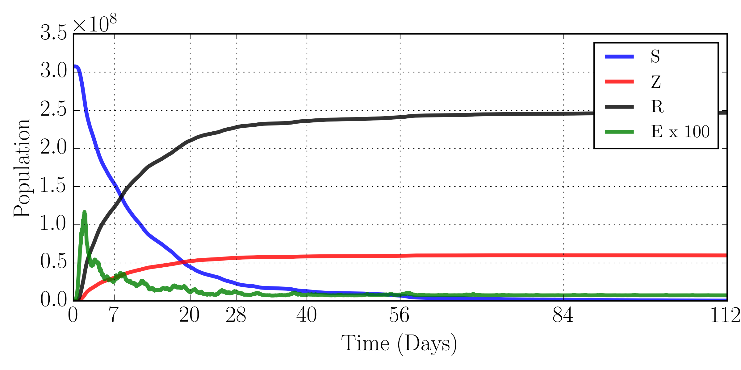
With the simulation in place, we are now in a position to simulate a full scale zombie outbreak. We first consider an outbreak that began with one in every million individuals starting in the Exposed () state in the United States. For a single instance the overall populations are shown in Figure 10. This looks similar to the analytical outbreaks we saw in Figure 1, but with a steeper rate of initial infection and some slight perturbations to the curves. The total population curves however hide most of the interesting features. In Figure 11 we attempt to give a sense of how this outbreak evolves, showing the state of the United States at various times after the outbreak begins.


As you can see, for the parameters we chose, most of the United States population has been turned into zombies by the first week, while the geographic map does not necessarily seem all that compelling. In the early stages of the outbreak, while the population is roughly homogeneous, the zombie plague spreads out in roughly uniform circles, where the speed of the infection is tied to the local population density. Infestations on the coasts, with their higher population density, have spread farther than those near the center of the country. After several weeks, the map exhibits stronger anisotropy, as we spread over larger geographical areas and the zombie front is influenced by large inhomogeneities in population density. After four weeks, much of the United States has fallen, but it takes a very long time for the zombies to diffuse and capture the remaining portions of the United States. Even four months in, remote areas of Montana and Nevada remain zombie free.
To investigate the geographical characteristics of the outbreak, we must move beyond a single instance of an outbreak and study how different regions are affected in an ensemble of outbreaks. If it takes a month to develop and distribute an effective vaccine (or an effective strategy for zombie decapitation), what regions should one locate the zombie-fighting headquarters? We ran 7,000 different 28-day zombie outbreaks in the continental United States starting with a single individual. A single instance of one of these outbreaks originating in New York City is shown in Figure 12.


By averaging over all of these runs, we can start to build a zombie susceptibility map, as shown in Figure 13. In the top plot, we show the probability that the given cell is overrun by zombies after seven days. Here you can clearly see that there are certain regions – those surrounding populous metropolitan areas – that are at a greater risk. This is partly because those regions have lots of individuals who could potential serve as patient zero, and partly due to the rapid spread of zombies in those areas. In the bottom plot, we plot the probability that the cell is overrun, but at the 28 day mark.
After 28 days, it is not the largest metropolitan areas that suffer the greatest risk, but the regions located between large metropolitan areas. For instance, in California it is the region near Bakersfield in the San Joaquin Valley that is at the greatest risk as this area will be overrun by zombies whether they originate in the San Francisco area or the Los Angeles / San Diego area. The area with the greatest one month zombie risk is north eastern Pennsylvania, itself being susceptible to outbreaks originating in any of the large metropolitan areas on the east coast.
VI Conclusion
Zombies offer a fun framework for introducing many modern concepts from epidemiology and critical phenomena. We have described and analyzed various zombie models, from one describing deterministic dynamics in a well-mixed system to a full scale US epidemic. We have given a closed form analytical solution to the well-mixed dynamic differential equation model. We compared the stochastic dynamics to a comparable density-dependent model. We investigated the critical behavior of the single person per site two-dimensional square lattice zombie model and demonstrated it is in the percolation universality class. We ran full scale simulations of a zombie epidemic, incorporating each human in the continental United States, and discussed the geographical implications for survival.
While this work is predicated on a fictional infestation, one might ask whether there are any phenomena in the real world that behave in a manner similar to our modeled zombie outbreaks. As noted, the model requires that susceptible hosts directly participate in the removal of zombie hosts from the infectious population, leading to runaway outbreaks as susceptible hosts are depleted. One might imagine a similar phenomenon for infectious diseases that require medical intervention to be suppressed; as medical personnel themselves become infected (as has sadly happened to a considerable degree during the recent Ebola outbreak in West Africa), they become less able to stem the spread of infection. (Medical personnel, however, represent only a small fraction of all susceptible hosts, so a refinement to an -type model would be required to account for this.) One might also imagine -like dynamics in the spread of ideas and opinions: a person spreading a controversial opinion in a population, for example, might be able to sway some converts, but is also likely to meet resistance and counter-arguments, which act to reduce infectivity and perhaps ultimately stop the spread.
We hope our systematic treatment of an imaginary disease will provide a useful and inspiring teaser for the exciting fields of statistical mechanics, network science, and epidemiology.
VII Acknowledgments
We acknowledge NSF IIS–1247696 and Cornell University for support of this research, and thank Paul Ginsparg for useful references and conversations.
References
- [1] Max Brooks. The Zombie Survival Guide: Complete protection from the living dead. Broadway books, 2003.
- [2] Max Brooks. World War Z. Querido’s Uitgeverij BV, Em., 2013.
- [3] John L Cardy and Peter Grassberger. Epidemic models and percolation. Journal of Physics A: Mathematical and General, 18(6):L267, 1985.
- [4] Andrew Cartmel et al. Mathematical Modelling of Zombies. University of Ottawa Press, 2014.
- [5] Jin Fu, Sheng Wu, Hong Li, and Linda R Petzold. The time dependent propensity function for acceleration of spatial stochastic simulation of reaction–diffusion systems. Journal of Computational Physics, 274:524–549, 2014.
- [6] Michael A Gibson and Jehoshua Bruck. Efficient exact stochastic simulation of chemical systems with many species and many channels. The journal of physical chemistry A, 104(9):1876–1889, 2000.
- [7] Daniel T Gillespie, Andreas Hellander, and Linda R Petzold. Perspective: Stochastic algorithms for chemical kinetics. The Journal of chemical physics, 138(17):170901, 2013.
- [8] Peter Grassberger. On the critical behavior of the general epidemic process and dynamical percolation. Mathematical Biosciences, 63(2):157–172, 1983.
- [9] Ronald Hochreiter and Christoph Waldhauser. Zombie politics: Evolutionary algorithms to counteract the spread of negative opinions. arXiv preprint arXiv:1401.6420, 2014.
- [10] Matt J Keeling and Pejman Rohani. Modeling infectious diseases in humans and animals. Princeton University Press, 2008.
- [11] Bruno Mota. Optimum survival strategies against zombie infestations-a population dynamics approach. Bulletin of the American Physical Society, 59, 2014.
- [12] Philip Munz, Ioan Hudea, Joe Imad, and Robert J Smith? When zombies attack!: mathematical modelling of an outbreak of zombie infection. Infectious Disease Modelling Research Progress, 4:133–150, 2009.
- [13] Mark EJ Newman, I Jensen, and RM Ziff. Percolation and epidemics in a two-dimensional small world. Physical Review E, 65(2):021904, 2002.
- [14] http://mattbierbaum.github.io/zombies-usa/.
- [15] https://github.com/meetar/dotmap.
- [16] Felipe Nunez, Cesar Ravello, Hector Urbina, and Tomas Perez-Acle. A rule-based model of a hypothetical zombie outbreak: Insights on the role of emotional factors during behavioral adaptation of an artificial population. arXiv preprint arXiv:1210.4469, 2012.
- [17] U.S. Department of Health, Human Services Centers for Disease Control, and Prevention. Preparedness 101: Zombie pandemic. http://www.cdc.gov/phpr/zombies/.
- [18] U.S. Department of Health, Human Services Centers for Disease Control, and Prevention. Preparedness 101: Zombie apocalypse. http://blogs.cdc.gov/publichealthmatters/2011/05/preparedness-101-zombie-apocalypse/, 2011.
- [19] Evelyn Sander and Chad M Topaz. The zombie swarm: Epidemics in the presence of social attraction and repulsion. Mathematical Modelling of Zombies, page 265, 2014.
- [20] Robert Smith? Braaaiiinnnsss!: From Academics to Zombies. University of Ottawa Press, 2011.
- [21] Tânia Tomé and Robert M Ziff. Critical behavior of the susceptible-infected-recovered model on a square lattice. Physical Review E, 82(5):051921, 2010.
- [22] Caitlyn Witkowski and Brian Blais. Bayesian analysis of epidemics-zombies, influenza, and other diseases. arXiv preprint arXiv:1311.6376, 2013.