Clues for flavor from rare lepton and quark decays
Abstract
Flavor symmetries successfully explain lepton and quark masses and mixings yet it is usually hard to distinguish different models that predict the same mixing angles. Further experimental input could be available, if the agents of flavor breaking are sufficiently low in mass and detectable or if new physics with non-trivial flavor charges is sufficiently low in mass and detectable. The recent hint for lepton-nonuniversality in the ratio of branching fractions over , , suggests the latter, at least for indirect detection via rare decays. We demonstrate the discriminating power of the rare decay data on flavor model building taking into account viable leptonic mixings and show how correlations with other observables exist in leptoquark models. We give expectations for branching ratios and , and Higgs decays .
I Introduction
The LHCb collaboration [1] has presented recent data on lepton-nonuniversality (LNU): , the ratio of branching fractions over , has been measured as
| (1) |
in the dilepton invariant mass squared bin , which represents a deviation of from lepton universality [2]. In view of its generic leptoquark interpretation [3] we investigate directions in flavor model building that link the electron-muon non-universality to other flavor observables particularly lepton masses and mixing and lepton-flavor violation (LFV). In general if LNU is present, LFV can be expected, too [4]. has also been addressed within (composite) leptoquark models [5]; they do not aim at explaining LFV. Also recently, [6] considered scalar leptoquark contributions to rare leptonic meson decays.
Here we consider frameworks where both phenomena (LNU, LFV) stem from the same (scalar) sector. To be more specific, we investigate the possibility of simultaneously accommodating LNU as observed through , and LFV, as observed in neutrino mixing and as hinted at 2.5 by CMS in [7]. We do so by adapting frameworks with non-Abelian flavor symmetries that predict the leptonic mixing matrix.
Due to the Standard Model (SM) gauge group, the maximal flavor symmetry is an for each chiral quark and lepton species. This observation motivates the use of or subgroups. After discussing briefly a framework of leptoquarks within the continuous group , [8] we consider explicit realizations with the discrete group in frameworks within supersymmetry (SUSY) [9, 10, 11, 12]. While the specific results are related to the details of the models, our general conclusion is generic even if other discrete subgroups of are invoked. If the same flavor symmetry breaking fields, often referred to as flavons, are involved in Higgs and leptoquark couplings, the respective Yukawa structures are related and there are links between what is predicted for LNU and LFV (in lepton mixing and Higgs decays).
The paper is organized as follows: in Section II we identify viable, data-driven patterns for flavor structure of the leptoquark to fermions coupling matrix. Predictions for rare LFV decays of leptons and -mesons are given in Section III. The results of these sections are rather independent of flavor models. In Section IV these benchmarks are compared to what is realized in theoretical flavor models, where we consider models based on and known for explaining lepton flavor. Rare Higgs decays are addressed in Section V. In Section VI we conclude. In several appendices we give formulae and auxiliary information.
II Data-driven flavor patterns
We consider models with a scalar doublet leptoquark , with electric charges and one with a scalar triplet leptoquark , with electric charges . Such frameworks correspond to the RL model and the LL model, respectively, of [3], which discussed them as “single particle” explanations of . For this reason, apart from having renamed the leptoquarks as , throughout this section we use the notation from [3].
In view of the uncertainties in the current data in the following we neglect factor of differences in the semileptonic 4-fermion operators after Fierz-ordering and other small differences between the RL and LL model variants. This way the phenomenological constraints on the leptoquark parameters relevant to our study give identical hierarchies in flavor patterns, which we hence study jointly. We stress that despite the present day patterns being similar, there are differences in terms of model-building. The -doublet leptoquark model couples to right-handed quarks 11 1 The RL model has similarities with the R-parity violating minimal supersymmetric standard model (MSSM); the corresponding term is the coupling. Note also that the with mass much lighter than the GUT-scale does not require further model-building to avoid proton decay [13].
| (2) |
while the -triplet leptoquark model couples to left-handed quarks
| (3) |
In each case, the couplings to the leptons are left-chiral and quark and lepton denote flavor (generation) indices. We denote the mass of the leptoquark by .
We continue discussing constraints on the generalized Yukawa for and :
implies at 1 [3]:
| (8) |
We restrict our analysis to TeV to be conservative with collider bounds [14, 15, 16, 17], hence, in view of Eq. (8), .
There is also a contribution to mixing from a box diagram with leptons and leptoquarks in the loop giving rise to an operator of the form with the complex coefficient . Numerically,
| (9) |
where the weaker bound is obtained from the mass difference , whereas the stronger one in parentheses stems from the upper bound on the mixing phase (defined relative to the SM phase in the decay amplitude) [18]. The complementarity of the and constraints allows to fix the mass scale and the dimensionless couplings separately, yielding an upper limit TeV. Couplings to different quark flavors are within four orders of magnitude, [3].
The simplest scenarios are when the leptoquark couples to one generation of leptons only, as considered in [3]. In this case reads,
A third variant with couplings to only cannot explain non-universality between electrons and muons as hinted currently by data. With either of those limits, or , there is no LFV in rare processes. 22 2 Generically can be explained by a suppressed branching ratio to muons, or an enhanced one to electrons, or combinations thereof, the details of which driven by an underlying model of flavor. Present data, however, is much more copious for rare decays into muons than into electrons due to the large data samples from the hadron machines at Fermilab and CERN LHC. This is likely to change in the nearer term future with the Belle II experiment taking data. As a consequence at present the constraints on the modes are much more loose. In addition, hints for new physics in angular distributions could point to a simultaneous explanation with , see [19] and references therein. So, the rather minimal scenario where originates at least predominantly from muon mode suppression and the electrons are SM-like presently has phenomenological support.
Generalizing the single lepton scenario we consider the hierarchical pattern
Here, we allow for quark flavor suppressions and having larger couplings for heavier generations. This is suggested by the observed quark mass pattern; see Appendix B for details on how this is realized with the Froggatt-Nielsen (FN) mechanism [20] from -flavor symmetries. Here we simply take typical phenomenological profiles for Higgs-Yukawas of quark doublets () and down-type singlets () from [21], and apply them to the leptoquark-Yukawa, leading to
| (21) |
where denotes a flavor parameter of the size of the sine of the Cabibbo angle, . We stress that what we mean by the hierarchies and flavor patterns in general is that they hold up to numbers (including CP phases) of order one. The overall scale in our ansatz () depends on and is fixed by through Eq. (8). 33 3 Note that here we do not explicitly specify charges for the leptons , whose assignments are not fixed by phenomenology as they depend on the model of neutrino masses. While in general the texture Eq.(̃II) with suppressions Eq.(̃21) is expected to hold, there is the possibility for cancellations between quark and lepton charges, that could lead to inverted hierarchies in the leptoquark Yukawa . We do not consider such solutions; they are absent as long as all charges are non-negative.
| observable | current 90 % CL limit | constraint | future sensitivity |
|---|---|---|---|
| [22] | [23] | ||
| [24] 44 4 In previous versions of this work this bound was incorrectly stated as , which reflected the abstract of the original version of [24] in the arXiv, which has been corrected in June 2015. | |||
| [25] | [26] | ||
| [27] | [26] | ||
| [28] | |||
| [14] | |||
| [14] | |||
| [29] |
We emphasize that our main goal is to simultaneously explain lepton mixing and LNU. Lepton mixing is structurally very different from the hierarchical quark mixing matrix, which suggests a different origin of flavor for the leptons. We therefore consider in Section IV scenarios where the entries between columns of are related by factors that are or as in Eq. (II). Such structures can occur naturally from a non-Abelian flavor symmetry distinguishing the generations of leptons. We state the set of assumptions that lead to an effective factorization of quark flavor (rows) and lepton flavor (columns) in : the Higgs, leptoquark and quarks are singlets under the leptonic flavor symmetries while leptons are neutral under the quark symmetries. Most scenarios we consider will be factorized, including the hierarchical ansatz Eq. (II). Therein the flavor parameter allows to split the electrons from the other leptons, and is further discussed together with LFV below. Although it is not completely general, the structure of is useful to obtain predictions, which we do in Section III, that can apply for more general flavor patterns, as shown in Section IV.4. Non-factorized scenarios are discussed in Section IV.3.1 and Appendices D, E.
If couplings to more than one lepton flavor are present, existing constraints on LFV processes need to be considered. In Table 1 we collect LFV data, the corresponding constraints on -matrix elements, and give future sensitivities whenever available. Constraints on couplings to -leptons exist from the -factory experiments Belle and Babar [24, 25, 27]. These bounds are not competitive with -physics ones but can be improved in the near term future at Belle II [26]. The strongest constraint on is therefore from -mixing Eq. (9). Consequently, phenomenology does not currently require a split (within our approximations) between muons and taus, which is why we refrain from adding a flavor factor separating the second and the third column of in Eq. (II). Note also that while it would be straightforward to implement such a factor, for leptoquark masses near maximal, already requires muon couplings of order one, cf. Eq. (8), so allowing significantly larger than would challenge perturbativity.
The strongest constraint on LFV stems from from MEG 2013
| (22) |
This is only mildly stronger than the bound Eq. (8), implying . The requirement of flavor hierarchies between electrons and muons can become more pronounced in the short-term future, with MEG upgrading their sensitivity to [23], which implies , if no signal is seen and remains close to its current determination. If the constraint tightens, it implies that in there has to be a dominant contribution to one lepton flavor with one branching ratio closer to its respective SM branching ratio than the other - ruling out solutions to Eq. (8) where and couplings are of roughly the same order of magnitude.
Current limits on LFV in -decays are also given in Table 1. They are weaker than Eq. (8). Comparison of the bound on with the one on , also shown, implies .
Rare kaon decay data provide the strongest constraint on couplings to -quarks [31]:
| (23) |
Due to chiral symmetry contributions from purely left-chiral leptons to the anomalous magnetic moment of the electron or the muons are much smaller than current experimental sensitivities.
To summarize, the phenomenologically viable range for parameters in Eq. (II) is
| (24) |
In view of , if (corresponding to a low mass leptoquark), then necessarily .
Regarding conversion in nuclei, the current best limit [32] is consistent with the bounds (24), however, future experiments such as COMET [33] and Mu2e [34] with sensitivity below are sensitive to the parameter space of leptoquark models discussed here55 5 We thank Franz Muheim for drawing our attention to future conversion experiments.. We note that corresponding tree-level contributions can always be avoided by decoupling down-quarks, suppressing , or decoupling electrons, suppressing .
Note that the model by [5] with the leptoquark being an triplet has a flavor structure , where the -powers are adjusted to give the correct fermion masses, similar to what could be obtained through a FN mechanism with -flavor symmetries. The resulting pattern turns out to be a viable subset of the one presented in Eq. (II). Specifically, and follow Eq. (21), and . Couplings to muons are mildly suppressed relative to the ones to taus, of the order , which is not far from our understanding of the symbol ’’ (within order one).
III LFV Predictions in terms of
The leptoquark framework with the ansatz from Eq. (II) is very predictive and allows for correlations between rare -decays and LFV. We obtain
| (25) | ||||
| (26) | ||||
| (27) |
and
| (28) | ||||
| (29) | ||||
| (30) | ||||
| (31) |
For the amplitudes of the purely leptonic decays note the chiral enhancement of over and . More general, neglecting phase space,
| (32) |
This relation follows from the left-handed lepton only hypothesis, a feature of the beyond SM (BSM) models considered here, see Appendix A for details. Eq. (32) can be used to test the lepton chirality in LFV processes.
Furthermore we obtain
| (33) | ||||
| (34) | ||||
| (35) |
where [35]. The current bound at 90 % CL by LHCb [36] is hence at least two to three orders of magnitude away.
In addition, for ,
| (36) |
Precise predictions for lepton flavor conserving decays we leave for future work. We stress that the calculation of the LFV hadron decays is much less complicated as contributions of quark loops or ()-resonances coupling to the electromagnetic current are absent.
There are two extreme scenarios assuming :
A) , corresponding to high mass leptoquark in the few TeV range, i.e., out of LHC reach. In this case can be of order one, too, implying that and could be just around the corner, cf. Table 1. Radiative -decays are far away while and are at least three orders of magnitude away from their respective current limits. , and .
B) , corresponding to light leptoquarks up to few TeV in mass and . As in scenario A), can be just around the corner, and is three orders of magnitude away from its current limit. , and are strongly suppressed, but can be found with the next round of experiments while remains far away.
C) , corresponding to light leptoquarks up to few TeV in mass. This scenario arises for instance in the model in Appendix B where the leptoquark carries FN charge to increase powers of spurion insertions. The LFV pattern follows from the values of as dictated by the flavor model.
Concerning collider searches within pattern Eq. (II) the leptoquark decays take place into second or third generation leptons and into third generation quarks. In scenario A), all combinations of quarks and leptons can arise at similar level except for those involving -quarks, which are necessarily suppressed.
In case of at least two more measurements rather than upper bounds on LFV in addition to the parameters and can be determined, pinning down the flavor pattern of the leptoquark coupling matrix further. It is conceivable that the latter is linked to the mechanism generating flavor for SM fermions, e.g., with flavor symmetries, which can be probed with the rare decay data. In Section IV we give examples of realistic flavor symmetries that give the single lepton flavor patterns Eq. (II), and special cases of the hierarchy pattern Eq. (II), but also further testable pattern. Predictions of leptoquark coupling patterns not covered by the ansatz Eq. (II) are given in Section IV.4.
IV Flavor symmetries
In this section we illustrate how flavor symmetries generically control the shape of the leptoquark Yukawa coupling matrix , and how there is in general a relation to Higgs Yukawa couplings controlled by the same symmetry. The reason for this is simply that both the leptoquark and Higgs doublet (or doublets) couple to same fermions, whose generations transform as specific representations of the flavor symmetry.
We use specific models to demonstrate this, and show how to obtain some special cases for , including , from Eq. (II), and from Eq. (II), but also new structrures.
In terms of the quark index in , the structure between rows depends on what kind of symmetry transformations we assign to either the generations (for the LL leptoquark) or to the RH down-type quarks (for the RL leptoquark). In frameworks where the flavor symmetry distinguishes and , the LL and RL leptoquark models could be very different. Here, we focus mostly on frameworks of flavor symmetries explaining leptonic mixing, where this is not the case. If we assume all quarks are trivial singlets of whatever non-Abelian symmetry is included, one can still assign a FN charge to quarks (under ) leading to Eq. (21) or similar. The FN mechanism relies on having lighter generations with larger charges in order to explain the mass hierarchies through added insertions of a field. We choose without loss of generality to normalize the charge of to . If we assume that the leptoquark is neutral under the , the leptoquark Yukawa couplings to lighter generations of quarks is simply suppressed by as many additional insertions of as the ones that appear for the respective masses, resulting in Eq. (21). We relegate further considerations of the charges of to Appendix B, in order to focus on the structure of the lepton couplings, where we consider non-Abelian flavor symmetries.
Before we delve exclusively into lepton flavor models, it is interesting to consider a SUSY framework with an underlying unified gauge group, where quark and leptons are linked. This is particularly restrictive in terms of the allowed flavor structures. At this level we will consider the flavor symmetry to be continuous (, Section IV.1).
We then investigate in some detail a SUSY framework with discrete flavor symmetry in Sections IV.2 and IV.3. We focus on because it is a convenient framework to obtain the observed pattern of leptonic mixing, but also due to its relative simplicity as the smallest group with triplet representations. Appendix C contains a brief primer on .
The reason for having SUSY in all the frameworks discussed in this section is twofold: first, SUSY keeps the gauge hierarchy problem under control, which is particularly relevant when going beyond the SM (with or flavor symmetries broken at a high scale). Second, by holomorphy it allows one to separately align the different flavor symmetry breaking directions required in the respective models. Because of SUSY, we necessarily use two doublets, and .
All the frameworks also have a R-symmetry, which is spontaneously broken to its subgroup acting like the MSSM R-parity. Another point that all the frameworks we consider have in common is the presence of an auxiliary Abelian flavor symmetry (either , or ). As a point of notation, in each section the charge of a superfield under the relevant auxiliary symmetry is denoted as .
IV.1 unified framework
We discuss now a framework exemplified by the model presented in [8]. Similar models were considered in [37, 38], showing how to obtain large reactor angle (). One of the main features in the framework are that the 3 generations of each fermion flavor transform as triplets of .66 6 Due to the underlying unification, if the 3 generations of lepton doublets transform as triplets, so must the generations of other SM fermions, as each generation is unified into a -plet of .
In order to build flavor symmetry invariants, we add three flavons (each with 3 generations) named , and (the subscript numbers are labels, the upper indices are generation indices , anti-triplet indices of ). Through the details of the superpotential of the model, the flavons acquire vacuum expectation values (VEVs), breaking the flavor symmetry in specific directions:
| (37) |
with . This VEV hierarchy is required to be of order of the Cabibbo angle, but is also related to the hierarchy between the solar and atmospheric neutrinos [8] and even to the magnitude of the reactor angle [38].
After is broken to a left-right symmetric GUT containing (before breaking to the SM), the left-handed fermions are referred as and the conjugates of the right-handed fermions as (where are generation indices, triplet indices of ), where contains the 3 generations of , and contains the 3 generations of and . The superfields containing the electroweak doublets we denote here as , .
The Yukawa couplings appear from non-renormalizable terms which are generally of the type and are controlled also by an auxiliary Abelian symmetry . The VEV directions in Eq. (37) are responsible for giving hierarchical structures for all the charged fermions.77 7 Refer to [8, 38] for the details related with getting viable mass ratios for the 2nd generation of fermions, such as at the GUT scale.
We focus now on the leptoquark Yukawa structures that occur naturally when leptoquarks are added to this framework. In order to study this, we need to keep in mind the transformation properties of the SM fermions, which are all triplets under , and the charges of the flavons under , which we denote in terms of curly brackets e.g. , and , while and the SM fermions are neutral, . To predict we simply need to select how transforms under . Here we discuss the simplest case where the leptoquark is an singlet. In Appendix D we consider leptoquark triplets under .
Note also that, due to the underlying unification and both transform equally under the flavor symmetry so there is no difference in the structures corresponding to a LL or RL leptoquark, and also that structures involving components from (, ) and () are symmetric due to their origin from the same multiplet. If we were considering a unified gauge group that is not left-right symmetric then the and would generally transform differently under the flavor symmetry and the structures for the RL and LL leptoquark would be different. A prime example of this is , where lepton doublets belong to the same GUT multiplet as , but is in a different GUT multiplet together with and . See Appendix E for some possibilities.
If is an singlet (as ), the flavor symmetry invariants shaping are , which are very similar to those shaping the fermion masses. Which particular flavons couple to is determined by its charge :
- •
- •
leads to .
- •
leads to two contributions: the dominant one and the subleading , shown together in Eq. (39).
- •
leads to .
- •
leads to , the democratic structure given in Eq. (40).
As we intend to account for , we show only the structures with non-zero entries simultaneously in , or simultaneously in , .
The flavor structure for reads
| (38) |
which is a highly predictive limit of Eq. (II) with the same exact magnitude on the 4 non-zero entries. As there is a single coupling we can absorb the order one coefficient by redefining .
Choosing gives
| (39) |
which due to has couple predominantly to . We kept explicit to separate leading and non-leading contributions and redefine to absorb the order one coupling of the subleading contribution, which, although suppressed by could in principle account for . However, the simultaneous presence of the kaon constraint Eq. (23) rules this out.
The democratic pattern from is
| (40) |
and very symmetric like , but it preserves lepton universality so it can not account for .
The only viable texture is therefore . In fact the only obtainable textures if there are only these 3 flavon VEVs are the textures explored so far. has no allowed couplings due to holomorphy, and for the only possibilities repeat the existing patterns as the matrix structure is driven only be the flavons contracting with and . Even at higher order it is not possible with this field content to obtain linear combinations of the textures. The reason for this is clearer when considering a specific example, so we skip as it has no allowed couplings, and take where:
| (41) |
is invariant, with the same texture as but with overall charge added due to singlet . Even though would allow to swap flavon contractions to and so on, all except Eq. (41) automatically vanish due to the Levi-Civita tensor.
IV.2 framework
The first framework we consider is of SUSY models, initially proposed in [9] and with renormalizable UV completions [11] and in particular [12] which obtains non-zero reactor angle in full agreement with current neutrino oscillation data. The FN mechanism [20] is implemented separately through , generating the hierarchy in the charged lepton masses without requiring small Yukawa couplings; it can easily be used to justify the quark hierarchies as described in Appendix B. SUSY’s holomorphy together with the separate the charged lepton sector and the neutrino sector. The triplet flavons and acquire vacuum expectation values (VEVs) in special directions and , respectively, shaping the leptonic mixing. The fields charged as under the R-symmetry are the alignment fields and are responsible for giving the flavons their VEV directions. We do not discuss the details of SUSY breaking, but when it occurs is broken to leave only a subgroup which distinguishes the SM fermions, i.e. it acts as R-parity. We refer to Table 2 for details about the charge assignments.
| See text | |||||||||||||||||||
| 0 | See App. B | ||||||||||||||||||
| , | |||||||||||||||||||
We have not listed the representation of in Table 2 as it requires a more detailed discussion. As we have done for , we focus on the case where the leptoquark is an singlet. We consider triplet leptoquarks in Appendix D.
For completeness, we include here very briefly the charged lepton Yukawa couplings in the superpotential
| (42) |
where is a scale associated with the breaking of the flavor symmetry. Coupling to the VEV results in a diagonal mass matrix for the charged leptons where we can identify with , with and with .
For , the hypercharge differs for the LL and RL leptoquark. The Yukawa coupling to leptoquarks is associated with a renormalizable superpotential term that is either for doublet corresponding to Eq. (2) - or, with a triplet , one would have as a SUSY version of Eq. (3). The quark generation index is and the lepton generation index is . We assume that all three generations of doublet and singlet quarks are trivial singlets of . We consider singlet down-type quarks as an triplet in Appendix E as this case arises in unified models [39, 40] with .
The columns of are constrained because is an triplet. If the leptoquark is an singlet, the renormalizable leptoquark superpotential terms are no longer invariant. A contribution to appears at leading order (LO) from a non-renormalizable term where contracts with an triplet flavon. There are then three options for to transform under , and 4 non-equivalent ways to build an invariant:
- 1.
. Then isolates , as .
- 2.
. Then isolates , as .
- 3.
. Then isolates , as .
- 4.
couples equally to all lepton generations due to .
By coupling to the VEV , the different options for the leptoquark representation under lead to a single non-vanishing column for . Options 1. and 2. correspond respectively to explicit realization of the patterns in Eq. (II), whereas option 3. gives SM-like and is disfavored by the current LHCb measurement. Option 4., which occurs regardless of , preserves lepton universality at LO but as discussed later has a myriad of LNU couplings already at NLO.
For now we postpone option 4. and take the charge of to be (following notation used in other sections for Abelian charge). This choice means that at LO couples to SM fermions only through .
This is a non-trivial result that we emphasize: using the same non-Abelian flavor symmetry and VEVs that jointly predict viable lepton mixing with large angles, one can obtain automatically leptoquark flavor structures where LNU exists due to the isolation of a single lepton generation. This is consistent with the LNU in to decays, as shown in [3], where the isolation of the or generation was merely assumed.
This isolation of lepton generation takes place at LO in a generic expansion parameter of , where represents the flavons and the scale of new physics associated with the breaking of . This can be identified more precisely in specific UV completions [11, 12], where it may turn out the isolation is actually exact (due to e.g. missing messengers for NLO diagrams). Generically one may still associate next-to-leading order (NLO) effects to the presence of non-zero reactor angle , which fixes the expansion parameter .
With a sizable expansion parameter it is important to consider contributions beyond LO, i.e. terms featuring additional flavon insertions (of the triplet flavons or of , a of ). For the case that produces lepton isolation, multiple insertions of involve the combination which gives contributions to that can be reabsorbed into the LO one, due to its effective VEV; on the other hand both and carry non-trivial charge so they can only appear as multiples of 3 so the earliest contribution appears at NNNLO which is of the order , hence sub-percent. We conclude that in this case, contributions beyond LO can only change the structure of negligibly, and lepton isolation holds to a very good approximation.
When considering effects beyond LO it is relevant to reconsider option 4., where leads to LO lepton universality due to the coupling with . The always allows adding the neutral to this scenario, so there are NLO contributions involving . The effective VEVs of the combinations are respectively , . For , and are also allowed by . LNU indeed arises at NLO, with 4 terms each with distinct LNU structures. Closer inspection of constraints in particular Eq. (8) shows that deviations from lepton universality at order in the entries
| (43) |
are phenomenologically viable. We conclude that LNU at NLO gives a viable pattern for .
One could consider assigning quarks non-trivially under , however, in the present framework this leads to issues in obtaining viable quark masses and mixing. Instead we will explore this option further in a different framework, , in Section IV.3.1.
IV.3 framework
The SUSY framework [10] is another interesting framework. For its renormalizable UV completions see also [11], and [12] for considerations regarding large .
We start with a brief comparison with the framework discussed in the previous section: the first difference is that the VEV of the flavon triplet coupling to the charged leptons is now . The second one is with respect with the FN mechanism and fields - neither nor are present, with the charged lepton hierarchy being due to a field . 88 8 To avoid confusion with the of Section IV.2, we renamed this field to . In [10, 11, 12] the same field is named . The last difference is that the sector neutral under is the neutrino sector whereas with , the charged lepton sector was neutral. This is particularly relevant due to e.g. the flavon neutral under . 99 9 In this framework, the presence of allows viable for a region of parameter space that is not fine-tuned, as discussed in detail in [12].
| See text | |||||||||||||||||||
|---|---|---|---|---|---|---|---|---|---|---|---|---|---|---|---|---|---|---|---|
| , |
When adding a leptoquark to this framework one can again obtain LO structures like Eq. (II) by having the charge of be . At LO we have:
- 1.
. Then isolates as .
- 2.
. Then isolates as .
- 3.
. Then isolates as .
They are similar to options 1.,2.,3. of Section IV.2, modified slightly to account for the (0,1,0) direction of the VEV.
More significant differences arise beyond LO, because the neutrino sector is neutral. Given that , one is allowed to add it to the LO contribution thus constructing NLO contributions involving . This is similar to what we have seen in Section IV.2, although the effective VEVs of the combinations are now , .
In order to keep the model predictive, we assume now that the contributions to are forbidden by a partial UV completion where beyond LO terms are only allowed through singlet insertions (this is a natural consequence if triplet messengers are absent [12]). In this scenario the only relevant flavon beyond LO is , which is also neutral under the . NLO contributions come from one insertion of and NNLO contributions from two insertions of . The options for are:
- 1.
has LO coupling to , NLO coupling to electron, NNLO coupling to .
- 2.
has LO coupling to electron, NLO coupling to , NNLO coupling to .
- 3.
has LO coupling to , NLO coupling to , NNLO coupling to electron.
We illustrate these in matrix form, defining :
| (44) |
where we also parametrized the quark suppression factors as in Eq. (II) for a more direct comparison. The first pattern, cannot simultaneously accommodate and -mixing constraints unless TeV. The second one, corresponding to an inverted hierarchy with leptons flavor ordering of leptoquark couplings in opposite way as the one to the Higgs, and the third one, normal hierarchy (for electrons) are both viable. Phenomenological implications are summarized in Section IV.4.
To conclude, within it is possible to obtain special versions of Eq. (II). Note also that, if instead of we had considered a neutral flavon - which would be difficult to distinguish in terms of lepton mixing angles [12] - for the same LO contribution, replacing the 1” with the 1’ leads to swapping which lepton generation is coupling at NLO and at NNLO, i.e, effectively swapping in each matrix in Eq. (44) the with the terms. The resulting structures are different and can be tested experimentally. As a corollary of that, by having simultaneously both and one can obtain LO in one lepton generation and at NLO the other two, e.g. LO coupling to , NLO to and to . The variant with LO coupling to is viable only for leptoquark masses not exceeding a few TeV due to Eq. (8) and Eq. (9).
IV.3.1 Quarks non-trivial under
An interesting option that can be considered is to make different generations of quarks transform as different non-trivial singlets of . Consider option 1., 2., 3. of the framework. If all quark generations are the same (non-trivial) singlet, it just shifts which lepton generation is isolated at LO by each leptoquark choice. For instance, if are all , then is the leptoquark that would now couple to , whereas which previously isolated would now couple instead to .
On the other hand new flavor pattern arise when different generations of quarks are transforming under different singlets. We note that some care is necessary as this possibility may lead to unwanted implications for the Yukawa couplings with the Higgs and a CKM matrix that is not viable. Indeed this is generally the case for the framework.
What happens with different generations of quarks assigned as different singlets is that, depending on the quark generation, the leptoquark couples to different columns at each order. As an illustration of this, and neglecting the quark FN charges for simplicity, take , still as trivial singlets but . We have at LO:
| (45) |
corresponding to:
| (46) |
Such patterns generalize lepton flavor isolation Eq. (II), and at the same time are no longer special limits of Eq. (II). The pattern Eq. (46) could be distinguished from the others for instance through the tree-level decays of the leptoquark in colliders.
Viable masses for quarks can be obtained for this type of assignments under as long as there are flavons allowing invariants populating the respective columns of the Yukawa coupling to the Higgs, . This is not the case for the framework, but in the framework considered in this section the neutral flavon allows it. For the example considered above where , terms populating with can be obtained through a double insertion of the flavon (note that if there is a FN charge of it should be amended with the additional flavon insertions in mind cf. Appendix B). For this reason, choices leading to non-trivial under are unappealing from a theoretical standpoint, as having the top quark mass arise from a renormalizable term is preferable.
In general, constructions of this type yield patterns for where a single quark flavor can couple to a single lepton flavor. Due to , either electrons or muons have to couple to both and . Therefore, the following structures in addition to Eq. (46) are phenomenologically viable:
| (47) |
All of these effective two-flavor patterns predict LFV involving two lepton flavors only at LO, but receive respective NLO (and NNLO) contributions which are similarly shifted in the first row and are also themselves a two-flavor pattern.
However, in specific UV completions it is possible to forbid NLO and NNLO contributions to , while allowing the desired LO contributions and the necessary Yukawa couplings. 1010 10 A relatively simple possibility for RL leptoquarks is to forbid triplet and singlet messengers. We have checked in this case the absence of pattern-changing beyond-LO diagrams, while the required diagrams for RL leptoquark Yukawa couplings and the Yukawa to quarks and charged leptons are mediated by doublets. In fact, allowing only a minimal set of messengers we can obtain matrices like Eq. (46) with , corresponding to the truly minimal patterns from [3] that explain LNU data Eq. (1).
IV.4 Summary of flavor symmetry frameworks and predictions
We summarize in Table 4 the features of the and frameworks discussed in the previous sections, for a single leptoquark.
| structure | symmetry | flavons | assignment |
|---|---|---|---|
| Eq. (II) with zeros, i.e. Eq. (38), | |||
| Eq. (II), electrons only | 1, | ||
| Eq. (II), muons only | 1”, | ||
| Eq. (II) with , i.e. Eq. (43), | , | ||
| Eq. (II), normal hierarchy, i.e. Eq. (44) | , | 1’, | |
| Eq. (II), inverted hierarchy, i.e. Eq. (44) | , | 1”, | |
| Eq. (46) , Eq. (47) two-flavor | 1’ , |
The phenomenology of the patterns following from the hierarchy ansatz Eq. (II) has been detailed in Section III. The two-lepton flavor patterns Eq. (46) and Eq. (47) discussed in Section IV.3.1 that arose newly in the analysis of the flavor symmetries, have predictions similar to the single lepton flavor pattern Eq. (II): they successfully explain by either BSM in or transitions, however LFV signals can appear in addition in either , or related to or transitions. For the example in Eq. (46): , and , but none involving electrons. The sub-case for , that is no couplings to -quarks, can also be obtained, corresponding to the minimal benchmark patterns presented in [3], to which we refer for their phenomenology. They have no LFV. Implications include effects in decays, relevant for the Belle II experiment. Correlations between and have been worked out in [41].
The other genuine non-Abelian type of structure is the inverted hierarchy Eq. (44), , in which the leptoquarks couplings do not follow the ones of the leptons to the Higgs. This pattern predicts LFV in processes involving , and , which can be read off from the estimates given in Section III using , and , respectively. The normal hierarchy pattern, of Eq. (44), predicts LFV in processes involving , and corresponding to , and , respectively. In these cases, .
While it appears that it is possible to obtain in each flavor model pattern for RL and LL leptoquarks alike, we stress that this is a feature of the specific frameworks considered where and transform equally under the flavor symmetry, either due to underlying unification or for the sake of simplicity.
V Rare Higgs decays
In this section we discuss leptoquark effects in decays of the Higgs into fermion anti-fermion. Such decays have received recent interest with the advent of such a particle and its various decay modes being stringent test of the flavor sector of the SM and beyond, e.g., recently, [42, 43].
Leptoquark contributions to Higgs decays are induced at one-loop as exemplified in Figure 1. The amplitude is proportional to a renormalizable term , whose coefficient in general is model-dependent. After electroweak symmetry breaking a coupling of the Higgs to two leptoquarks is induced at order , where GeV sets the electroweak scale. The corrections to flavor-diagonal modes are hence parametrically given as
| (48) |
where denotes the number of colors. Analogously for :
| (49) |
Contributions from further one-loop diagrams involving the Higgs-Yukawa couplings exist but are suppressed further by at least , and contributions with don’t bring in additional enhancements either. The relative corrections to the diagonal Higgs Yukawas therefore do not exceed the level.
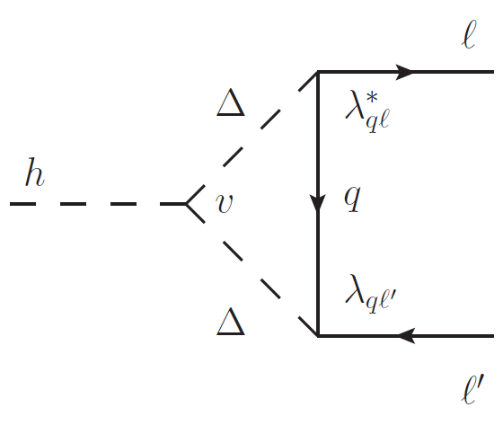
Spurion analysis shows when LFV in the Higgs coupling is induced, cf. Eq. (2),
| (50) |
hence the leptoquark couplings, in general, induce LFV couplings. A single Higgs doublet as in the SM suffices. Note that single lepton-flavor patterns as in Eq. (II) fail to induce for .
Leptoquark contributions to the -term in the spurion expansion arise at order
| (51) |
is suppressed relative to by for .
The coupling in Eq. (51) is the same which drives . We find that, using the limits from Table 1, LFV Higgs effects are limited as
| (52) |
Flavor models of course predict patterns for these couplings and relate decays. E.g., in terms of the parametrization Eq. (II):
| (53) |
If is large, this implies that all LFV branching ratios are strongly suppressed due to the suppression of . If is small, the branching ratio is much larger than the ones involving electrons. Different patterns follow from other flavor structures of summarized in Section IV.4.
The CMS data on the branching fraction [7] imply a sizable off-diagonal Yukawa-coupling to the SM-like Higgs , about a third of the coupling to the taus itself, . Such a sizable effect, taken at face value, exceeds the leptoquark estimates Eq. (52) and points to mechanisms beyond perturbative loops. An example is given by [44, 45].
VI Conclusions
The bottom-up BSM scenario with leptoquarks considered here provides further evidence of how new physics can help to learn about flavor [46]: if the anomalous signatures in the FCNCs Eq. (1) hold they offer unique possibilities to probe the mechanism of flavor, such as the type and charge assignment of a flavor symmetry whose imprints on SM matter were the only experimental information previously available.
By adding a leptoquark to existing flavor symmetry frameworks we obtained sample scenarios where the flavor symmetries are simultaneously responsible for LNU () and LFV, drawing in each case relations to the lepton mixing angles and charged fermion hierarchies predicted in these models.
The predictions for LFV lepton and -decays are copious, and we summarize them in Sections III and IV.4. The LFV branching ratios, whose size is driven by are in part accessible to near-term future experiments, including MEG, LHCb and Belle II, the details of which depend on the specific flavor pattern of the leptoquark coupling , single lepton flavor Eq. (II), the hierarchy pattern Eq. (II), or further patterns which follow from the non-Abelian nature of the underlying flavor symmetry. Viable and realistic ones are summarized in Table 4. They can be distinguished phenomenologically. Further data could not only be a discovery of BSM, but also provide clues about flavor. Already current data rules out many choices of flavor group assignments, as demonstrated in Section IV.
Indeed if certain patterns of leptoquark coupling are observed in the future, they constitute strong hints of the presence of non-Abelian flavor symmetries. From the examples studied in this paper we single out three patterns. One is predicted in the unified framework, and is highly symmetrical with four entries of the same magnitude, Eq. (38). Alternatively if lepton isolation, either in electrons on muons, Eq. (II), is observed to below percent level, that points to models such as our which only allow deviations from isolation at the NNNLO - or, given an appropriate UV completion, to models like our . Mimicking these patterns without using non-Abelian symmetries would require rather unnatural leptoquark couplings.
If LNU and LFV in rare -decays is observed, it allows to completely identify the chirality-structure of the leptoquark-lepton-quark couplings: comparison of with related non-universality tests into others strange final states, such as allows to probe for right-handed quark currents [47]. Specifically, the models Eq. (2) and Eq. (3) can be distinguished. Pinning down the chirality of the leptons is possible by comparing the LFV branching ratios with , which pick up different lepton mass factors. This method of diagnosing quark and lepton chirality, of course, applies model-independently for the low energy theory Eq. (54), i.e., is not limited to leptoquark mediated FCNCs.
The current hint for BSM in transitions in provides an anchor for fixing BSM scales when interpreted as a “signal” and combined with (-mixing) bounds. The mass range of the leptoquarks is determined to be right above search limits around and below TeV [3]. In collisions the leptoquarks will be pair-produced and decay in our frameworks predominantly into second or third generation leptons and into third generation quarks.
Note added: During the completion of this work a paper [48], appeared, where related leptoquark effects to were considered.
Acknowledgements
This project is supported by the European Union’s Seventh Framework Programme for research, technological development and demonstration under grant agreement no PIEF-GA-2012-327195 SIFT (IdMV) and by the DFG Research Unit FOR 1873 “Quark Flavour Physics and Effective Field Theories” (GH). The authors would like to thank the organizers of the NExT workshop 2014 "News from BSM, Higgs and Supersymmetry" at U. of Sussex, where this project was initiated.
Appendix A Leptoquarks in -decays
This appendix explains how to obtain predictions for -decays from the leptoquark interactions Eq. (2) and Eq. (3), corresponding to and , respectively. After integrating-out and fierzing [31], transitions with and are induced. Employing the common effective Hamiltonian
| (54) |
where , and denote the fine structure constant, the CKM matrix elements and Fermi’s constant, respectively, the semileptonic operators
| (55) | ||||
| (56) |
receive leptoquark contributions as [3]
| (57) |
Note that shows that the leptons are left-handed.
The amplitude for decays is calculated as
| (58) |
where we used that the hadronic matrix element is proportional to the mesons’ four-momentum, which equals the sum of the leptons’ four-momenta , and then applied the equations of motion for particle and anti-particle spinors . For same flavor leptons therefore the vector current contribution vanishes and using Eq. (57) the r.h.s. of Eq. (58) reads , with proportionality given by the anti-particle mass. Right-handed leptons, corresponding to would give instead the mass of the negatively charged lepton as chiral factor.
The model-independent framework Eq. (54), Eq. (57) allows to compute leptoquark effects in decays in a straightforward way. Correlations of the global fits and in such models have been discussed recently in [3, 5]. A detailed exploration including the very recent, preliminary data by LHCb on angular observables [49] taking into account SM uncertainties is beyond the scope of our work.
Appendix B Quarks and Froggatt-Nielsen
Relative suppression between rows of is naturally obtained by assigning different charges to the generations of quarks. The outcome depends also on the charge of the leptoquark. In this appendix curly brackets denote the charge of a field.
Explicitly, take the leptoquark triplet, and respectively [21]. The leptoquark couplings would be:
| (59) |
where . are order one dimensionless couplings. The outcome is an hierarchy between rows of the leptoquark couplings as e.g. , irrespective of lepton flavor. One can easily generalize this for alternative assignments of FN charges, such as [21], and similarly for the leptoquark doublet, where or [21]. Values for suppression factors of strange quarks versus -quarks, , and down quarks versus -quarks, , can be read-off and are compiled in Eq. (21). In this framework , consistent with the bounds Eq. (24).
Choosing non-zero values of FN-charges for the leptoquark significantly impacts and the resulting phenomenology, which forces to be within 0 and : adds an overall suppression to all leptoquark couplings of , which, while keeping unchanged, leads to suppression of . This requires lighter leptoquarks to explain . This case is discussed in scenario C of Section III. Too large charges cannot accommodate simultaneously Eq. (8) and direct search limits TeV. Within SUSY negative charges are in conflict with Eq. (8), because due to holomorphy, forbids couplings to -quarks. To see this take and compare to or , which are zero to account for the mass of the and top quarks.
Appendix C A few details
has 4 distinct irreducible representations, three of them are 1-dimensional, i.e. singlets, and one of them is 3-dimensional, i.e. the triplet. The trivial singlet we label , and it transforms trivially under . The (non-trivial) singlets and are conjugate to one another and they transform under a specific generator, , by getting multiplied respectively by and (, with ). The product of singlets has , , transforming as , , and respectively. The action of the group on triplets is represented by matrices. Consider specific triplets , . Under generator , which is diagonal in the basis we are considering, we have (same for ). We use the conventions in [11, 12], and square brackets to indicate products:
| (60) | ||||
| (61) | ||||
| (62) |
It is also possible to construct a symmetric () and an anti-symmetric () triplet:
| (63) |
Appendix D (Anti-)triplet
Within the frameworks we considered in Section IV it also possible to consider 3 generations of leptoquarks transforming as a representation of the flavor symmetry. This is more intricate than the single leptoquark scenarios we focused on, as there are three structures (one for each generation of the multiplet), and the flavor structure of the mass matrix for the generations is also relevant. In the frameworks considered here only acquire masses after the R-symmetry is broken (the leptoquark mass terms behave similarly to the -term ). As we will show, in some cases there are holomorphic bi-linears that could couple to whatever superfield is responsible for breaking the R-symmetry.
D.1
In the framework one can have anti-triplet (i.e. 3 generations of leptoquark transforming like the ) or instead a triplet (i.e. 3 generations of leptoquark transforming like the SM fermions). Discussing full models is beyond the scope of the present paper, but we illustrate some structures that can arise.
For triplet , the invariants can be quite different from those discussed in section IV.1. If there is an invariant not involving the flavons . This is a purely anti-symmetric structure for each :
| (64) |
For this charge assignment there are no holomorphic leptoquark bi-linears to study, but we can nevertheless conclude that this type of structure can not account for regardless of the mass eigenstates.
If , invariants can arise by contracting to 3 flavons, such as :
| (65) |
which occurs for , where decouples and couple with , Eq. (38). For this charge assignment, there is a holomoprhic bi-linear . It could give rise to a mass contribution after the R-symmetry is broken:
| (66) |
Diagonalizing this mass matrix reveals has vanishing mass prior to soft terms, so we expect it to remain as the lightest leptoquark - however it also has no coupling to SM fermions. The next lightest mass eigenstate with mass mass , and the heaviest with mass , are respectively dominantly (with some ) and the orthogonal combination. As both couple to SM fermions with the texture, this option reduces to a more involved version of the singlet leptoquark discussed before.
For anti-triplet , the invariants require only a single flavon contraction (contrasting to fermion mass structures that required 2, and the anti-triplet which as we have seen requires either 0 or 3). An example would be for , where we have :
There is no contribution from holomorphic bi-linears, as vanishes. We can still conclude that these structures would allow for as long there are sufficiently light eigenstates containing .
D.2
If we have 3 generations of leptoquarks as an triplet there can be invariant contractions , if under , ; within the choice would be . Each generation has its own matrix. The LO-structures are:
| (77) |
The holomorphic bi-linears in allowed by are , and . This could lead to a mass structure
| (78) |
where we absorbed the magnitudes of the respective VEVs into the coefficients . This is similar to the Majorana neutrino structure in this framework (see [12]). With eigenvalue , is an eigenstate of this structure which, when compared to the respective , would preserve lepton universality. In the limit we have effectively and the other two eigenstates are also independent of the free parameters: they would be and , respectively with eigenstates and . These two leptoquark eigenstates could mediate LNU couplings. As it is that generates non-vanishing reactor angle in this framework, in realistic regions of parameter space the and directions are no longer eigenstates of the leptoquarks. is still possible and an interesting situation arises where the perturbations away from the and directions to the leptoquark mass eigenstates are directly related to and the required perturbations of the neutrino eigenstates, appearing in the leptonic mixing matrix (recall in this basis the charged leptons are diagonal).
Studying NLO corrections for the triplet , which requires correcting both the and the assumed structures for , is beyond the scope of the present work.
Appendix E as triplet
We consider here a situation where remains as singlets under the flavor symmetry but is, like , an triplet. This situation arises naturally in unified models of lepton mixing [39, 40] with . Viable down quark masses can be obtained with LO contractions to the flavon, with NLO corrections from non-trivial singlet flavons and the up sector enabling viable CKM mixing.
If one can have a RL leptoquark coupling with no flavon, , which depending on gives respectively structures:
| (79) |
This structure would appear for within and for within .
Another possibility would be to couple to , . For a VEV and , or alternatively for a VEV and , these structures correspond respectively to :
| (80) |
One of these can appear alone for the framework and , as . In the framework so the structure appears for , i.e. together with the respective structure for each choice - the choice having and the choice having , these are two more candidates that can justify .
The final possibility is to couple to , with VEV, through . correspond to
| (81) |
In the framework so the structure appears for , i.e. together with the respective structure for each choice . can appear for the framework and , as , but this also allows to couple to . Effectively this means that in both frameworks one must combine with one of the three .
References
- [1] R. Aaij et al. [LHCb Collaboration], Phys. Rev. Lett. 113, no. 15, 151601 (2014) [arXiv:1406.6482 [hep-ex]].
- [2] G. Hiller and F. Krüger, Phys. Rev. D 69, 074020 (2004) [hep-ph/0310219].
- [3] G. Hiller and M. Schmaltz, Phys. Rev. D 90, no. 5, 054014 (2014) [arXiv:1408.1627 [hep-ph]].
- [4] S. L. Glashow, D. Guadagnoli and K. Lane, arXiv:1411.0565 [hep-ph].
- [5] B. Gripaios, M. Nardecchia and S. A. Renner, arXiv:1412.1791 [hep-ph].
- [6] S. Sahoo and R. Mohanta, arXiv:1501.05193 [hep-ph].
- [7] V. Khachatryan et al. [CMS Collaboration], arXiv:1502.07400 [hep-ex].
- [8] I. de Medeiros Varzielas and G. G. Ross, Nucl. Phys. B 733, 31 (2006) [hep-ph/0507176].
- [9] G. Altarelli and F. Feruglio, Nucl. Phys. B 741, 215 (2006) [hep-ph/0512103].
- [10] G. Altarelli and D. Meloni, J. Phys. G 36, 085005 (2009) [arXiv:0905.0620 [hep-ph]].
- [11] I. de Medeiros Varzielas and L. Merlo, JHEP 1102, 062 (2011) [arXiv:1011.6662 [hep-ph]].
- [12] I. de Medeiros Varzielas and D. Pidt, JHEP 1303, 065 (2013) [arXiv:1211.5370 [hep-ph]].
- [13] I. Dorsner, S. Fajfer and N. Kosnik, Phys. Rev. D 86, 015013 (2012) [arXiv:1204.0674 [hep-ph]].
- [14] K. A. Olive et al. [Particle Data Group Collaboration], Chin. Phys. C 38, 090001 (2014).
- [15] CMS Collaboration [CMS Collaboration], CMS-PAS-EXO-12-041.
- [16] G. Aad et al. [ATLAS Collaboration], JHEP 1306, 033 (2013) [arXiv:1303.0526 [hep-ex]].
- [17] K. Wichmann [ZEUS Collaboration], PoS ICHEP 2012, 145 (2013).
- [18] Y. Amhis et al. [Heavy Flavor Averaging Group (HFAG) Collaboration], arXiv:1412.7515 [hep-ex].
- [19] T. Blake, T. Gershon and G. Hiller, arXiv:1501.03309 [hep-ex].
- [20] C. D. Froggatt and H. B. Nielsen, Nucl. Phys. B 147, 277 (1979).
- [21] P. H. Chankowski, K. Kowalska, S. Lavignac and S. Pokorski, Phys. Rev. D 71, 055004 (2005) [hep-ph/0501071].
- [22] J. Adam et al. [MEG Collaboration], Phys. Rev. Lett. 110, 201801 (2013) [arXiv:1303.0754 [hep-ex]].
- [23] A. M. Baldini et al., arXiv:1301.7225 [physics.ins-det].
- [24] K. Hayasaka et al. [Belle Collaboration], Phys. Lett. B 666, 16 (2008) [arXiv:0705.0650 [hep-ex]].
- [25] B. Aubert et al. [BaBar Collaboration], Phys. Rev. Lett. 104, 021802 (2010) [arXiv:0908.2381 [hep-ex]].
- [26] T. Aushev et al., arXiv:1002.5012 [hep-ex].
- [27] Y. Miyazaki et al. [BELLE Collaboration], Phys. Lett. B 648, 341 (2007) [hep-ex/0703009 [HEP-EX]].
- [28] B. Aubert et al. [BaBar Collaboration], Phys. Rev. D 73, 092001 (2006) [hep-ex/0604007].
- [29] B. Aubert et al. [BaBar Collaboration], Phys. Rev. Lett. 99, 051801 (2007) [hep-ex/0703018].
- [30] I. Dorsner, J. Drobnak, S. Fajfer, J. F. Kamenik and N. Kosnik, JHEP 1111, 002 (2011) [arXiv:1107.5393 [hep-ph]].
- [31] S. Davidson, D. C. Bailey and B. A. Campbell, Z. Phys. C 61, 613 (1994) [hep-ph/9309310].
- [32] W. H. Bertl et al. [SINDRUM II Collaboration], Eur. Phys. J. C 47, 337 (2006).
- [33] Y. G. Cui et al. [COMET Collaboration], KEK-2009-10.
- [34] L. Bartoszek et al. [Mu2e Collaboration], arXiv:1501.05241 [physics.ins-det].
- [35] C. Bobeth, M. Gorbahn, T. Hermann, M. Misiak, E. Stamou and M. Steinhauser, Phys. Rev. Lett. 112, 101801 (2014) [arXiv:1311.0903 [hep-ph]].
- [36] R. Aaij et al. [LHCb Collaboration], Phys. Rev. Lett. 111, no. 14, 141801 (2013) [arXiv:1307.4889 [hep-ex]].
- [37] I. de Medeiros Varzielas, JHEP 1201, 097 (2012) [arXiv:1111.3952 [hep-ph]].
- [38] I. de Medeiros Varzielas and G. G. Ross, JHEP 1212, 041 (2012) [arXiv:1203.6636 [hep-ph]].
- [39] I. de Medeiros Varzielas, S. F. King and G. G. Ross, Phys. Lett. B 648, 201 (2007) [hep-ph/0607045].
- [40] G. Altarelli, F. Feruglio and C. Hagedorn, JHEP 0803, 052 (2008) [arXiv:0802.0090 [hep-ph]].
- [41] A. J. Buras, J. Girrbach-Noe, C. Niehoff and D. M. Straub, arXiv:1409.4557 [hep-ph].
- [42] R. Harnik, J. Kopp and J. Zupan, JHEP 1303, 026 (2013) [arXiv:1209.1397 [hep-ph]].
- [43] A. Dery, A. Efrati, Y. Nir, Y. Soreq and V. Susic, Phys. Rev. D 90, 115022 (2014) [arXiv:1408.1371 [hep-ph]].
- [44] A. Crivellin, G. D’Ambrosio and J. Heeck, Phys. Rev. Lett. 114, 151801 (2015) [arXiv:1501.00993 [hep-ph]].
- [45] A. Crivellin, G. D’Ambrosio and J. Heeck, Phys. Rev. D 91, no. 7, 075006 (2015) [arXiv:1503.03477 [hep-ph]].
- [46] Y. Nir, arXiv:0708.1872 [hep-ph].
- [47] G. Hiller and M. Schmaltz, JHEP 1502, 055 (2015) [arXiv:1411.4773 [hep-ph]].
- [48] I. Dorsner, S. Fajfer, A. Greljo, J. F. Kamenik, N. Kosnik and I. Nisandzic, arXiv:1502.07784 [hep-ph].
- [49] The LHCb Collaboration [LHCb Collaboration], LHCb-CONF-2015-002, CERN-LHCb-CONF-2015-002.