An Ant Colony Optimization Algorithm for Partitioning Graphs with Supply and Demand
Abstract
In this paper we focus on finding high quality solutions for the problem of maximum partitioning of graphs with supply and demand (MPGSD). There is a growing interest for the MPGSD due to its close connection to problems appearing in the field of electrical distribution systems, especially for the optimization of self-adequacy of interconnected microgrids. We propose an ant colony optimization algorithm for the problem. With the goal of further improving the algorithm we combine it with a previously developed correction procedure. In our computational experiments we evaluate the performance of the proposed algorithm on both trees and general graphs. The tests show that the method manages to find optimal solutions in more than 50% of the problem instances, and has an average relative error of less than 0.5% when compared to known optimal solutions.
Keywords:
Ant Colony Optimization, Microgrid, Graph Partitioning, Demand Vertex, Supply Vertex, Combinatorial Optimization1 Introduction
In recent years the research in the field of smart grids has had a significant increase in exploring the concept of interconnected microgrids [1]. This approach has resulted in novel types of typologies for electrical grids and new aspects of such systems that should be considered. Some of the most prominent newly emerged problems are the maximizing of self-adequacy [2], reliability, supply-security [3] and the potential for self-healing [4] of such systems. In many cases the underlying optimization problems are of a very high complexity and can not be solved to optimality in polynomial time. Electrical grids are systems of gigantic size, which makes their optimization very hard from a computational point of view. Luckily, previous research has shown that for many systems it is not necessary to use highly detailed models; often simplified graph ones can give sufficiently good approximations to the original problem. The family of graph partitioning problems has proven to be closely related to power supply and delivery networks [5, 6, 7, 8, 9].
In a system of interconnected microgrids each microgrid is made as independent from the rest of the system as possible; this results in many positive characteristics. Some examples are the lower complexity of the entire grid and enhanced reliability of each of the microgrids due to the increased resistance to failures in other parts of the system. The term independent is used for the case when there is a minimum of power exchange between the connected microgrids. This property of the system is formally defined as the maximization of self-adequacy of interconnected microgrids. Recently, research has been conducted in developing algorithms for finding approximate solutions [2] to this problem. Previous research has also explored the closely related problem of efficient decomposition or islanding of large grids into islands with a balanced generation/load subject to specific constraints [10, 11]. Due to the large complexity and size of electrical grids, when attempting to model and optimize some global properties, it is frequently convenient to use simplified graph models. Such models often result in different versions of graph partitioning problems suitable for specific real life applications. Some examples are having a balanced partitioning [12], minimizing the number or weight of cuts [13, 14], or by limiting the number of cuts [15].
The focus of this paper is on the Maximal Partitioning of Graphs with Supply and Demand (MPGSD). The majority of previous research has been dedicated to the theoretical aspects of this problem [16, 17, 6, 18]. A significant part of the published work is focused on solving this problem for specific types of graphs like trees [17, 6, 18] and series-parallel graphs [16]. A method for finding solutions with a guarantee of a -approximation for general graphs has been presented in [9]. Different variations of the original problem have been developed, like a parametric version [19] and one with additional capacity constraints [20].
In this paper we present an ant colony optimization (ACO) [21] approach for finding high quality approximate solutions to the MPGSD. ACO has previously been successfully applied to problems of multiway [22] and balanced [23] graph partitioning. The same method has also proven to be suitable for the closely related problems of graph cutting [24] and covering [25, 26] and partitioning of meshes [27]. The proposed ACO adaptation for our problem of interest is based on the greedy algorithm presented in [28, 29]. The ACO algorithm is further improved by combining it with our previously developed correction procedure [29]. In our tests on general graphs and trees, we show that the newly developed method frequently manages to find optimal solutions and has a small average error when compared to known optimal solutions.
The paper is organized as follows. In the second section we give the definition of the MPGSD. Then we provide a short outline of a greedy algorithm which is used as a basis for the proposed method. In the third section we present details of our ACO algorithm. In the subsequent sections we discuss results of our computational experiments and provide some conclusions.
2 Maximal Partitioning of Graphs With Supply/Demand
The MPGSD is defined for an undirected graph with a set of nodes and a set of edges . The set of nodes is split into two disjunct subsets and . Each node will be called a supply vertex and will have a corresponding positive integer value . Elements of the second subset will be called demand vertices and will have a corresponding positive integer value . The goal is to find a partitioning of the graph that satisfies the following constraints. All the subgraphs in must be connected subgraphs containing only a single distinct supply node. As a result we have . Each of the must have a supply greater or equal to its total demand. Each demand vertex can be an element of only one subgraph, or in other words it can only receive ’power’ from one supply vertex through the edges of .
With the intention of having a simpler notation, we will use strictly negative values for demand nodes and positive values for supply nodes (note that this is slightly different from the definition of [16]). The goal is to maximize the fulfillment of demands, or more precisely to maximize the following sum.
| (1) |
while the following constraints are satisfied for all
| (2) | |||
| (3) | |||
| (4) |
An illustration of the MPGSD is given in Figure 1.
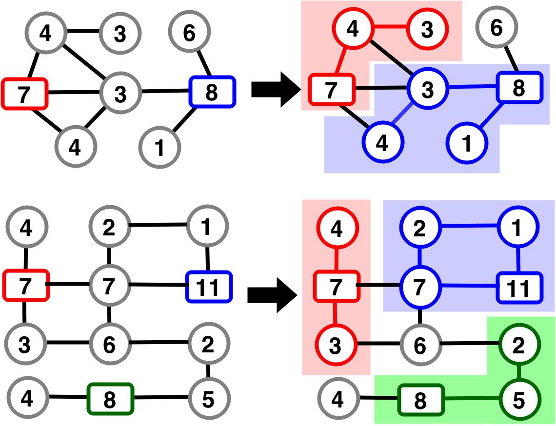
It has been shown that the MPGSD is NP-hard even in the case of a graph containing only one supply node and having a star structure [16].
3 Outline of Greedy Algorithm
In this section we give a short overview of the greedy algorithm, for which details can be found in [28], that is used as a base for the ACO method for the MPGSD. As previously stated, the solution of the problem of interest is a set of subgraphs where is the number of supply nodes. In the initial step of the algorithm we start with disjunct subgraphs , that only contain one supply node . At each of the following steps (iterations) of the algorithm one vertex is selected and used to expand a selected subgraph . The selection of both and is performed in a way that the newly generated subgraph satisfies the constraints of being connected, disjunct and fulfills Eq. 2.
Let us define as the set of adjacent vertices to in using the following equation
| (5) |
The idea is to gradually expand each of the subgraphs by adding new vertices to them. The set of potential candidates for expansion of subgraph , or in other words vertices that are adjacent to the , can be defined using the extension of to subgraphs. It is important to note that as the subgraph will be changed in subsequent iteration, the notation will be used to specify the state of subgraph at iteration . Now we can extend the definition of with the following equation.
| (6) |
It is evident that if the expansion of subgraph is done by the newly created subgraph will be connected, but it is not necessary that the other constraints will be satisfied. More precisely, the new need not satisfy Eq. 2, or there may exist such an that for the new subgraph. This can be avoided if instead of using set , we use a restricted set of vertices that guarantees that the constraints will be satisfied when is expanded using . We shall first define as the available supply for subgraph at iteration in the following equation.
| (7) |
Using given in Eq. 7, is defined in the following way.
| (8) |
The sets are used to specify the greedy algorithm for the MPGSD in combination with two heuristic functions. More precisely, at each iteration one heuristic is used to select the subgraph most suitable for expansion, and the second heuristic will be used to select the best to be added to . An extensive analysis of potential heuristics is given in our previous work given in articles[28, 29]. This procedure will be repeated until it is not possible to expand any of the subgraphs.
4 Application of Ant Colony Optimization
In this section we present an ACO approach for solving the MPGSD, based on the greedy algorithm from [28], outlined in the previous section. The general idea of ACO algorithms is to perform an "intelligent" randomization of an appropriate greedy algorithm for the problem of interest. There are several variations of ACO, out of which the Ant Colony System [30] is most commonly used. In it the "intelligence" comes from experience gained by previously generated solutions, which is stored in a pheromone matrix. In practice, a colony of artificial ants generates solutions using a probabilistic algorithm based on a heuristic function and the pheromone matrix. As in the case of the greedy algorithm, an ant generates a solution by expanding a partial one through steps. The difference is that instead of using a heuristic function it uses a probabilistic transition rule to decide what is to be added to the partial solution. The pheromone matrix stores the experience gathered by the artificial ants. This is done by applying a global and local update rule to the pheromone matrix. The global update rule is used after all ants in the colony have generated a solution and it reinforces the selection of elements inside of the best found solution or in some variations of good solutions. The local update is performed after an ant has applied the transition rule, and its purpose is to diversify the search of the solution space by avoiding the selection of the same elements of the solution by all of the ants.
Before defining the ACO algorithm for the MPGSD, we will first state some observations regarding the greedy algorithm and the form of the solution of the problem. A solution of the MPGSD can also be observed as a set of pairs , which states that node is inside subgraph . In this notation we will include for the case where is not a member of any subgraph . From this type of notation we realize that in the algorithm given in the previous section only the second stage, the selection of node , directly specifies the elements of the solution. The purpose of the heuristic in the first stage is to make it possible to perform a good expansion of the partial solution, which is of significant importance when only one solution is generated using a deterministic algorithm. In case of an ACO algorithm this becomes less important since many solutions are generated and the "steering" in the direction of good solutions is, to a large extent, done by the pheromone matrix.
Because of this, in the proposed ACO algorithm the heuristic function at this stage will be substituted with a random selection from the set of subgraphs that can be expanded. In this way the ACO mechanism will only be dedicated to the selection of expansion nodes.
4.1 Algorithm Specification
To specify the ACO for the MPGSD we need to define the transition rule, global and local update rules. In all of the following equations we will assume that we have a randomly selected subgraph with index . We will first define the transition rule, based on the same heuristic function as in [28], defined in the following equation.
| (9) |
The heuristic function given in Eq. 9 states that vertices with high demand are considered more desirable. The logic behind this is that it gets harder to satisfy high demands as the algorithm progresses since the available supply decreases as new vertices are added to the subgraphs. Because of this it is better to resolve high demands early.
Using we can define the transition rule for individual ants. This selection is done using a combination of deterministic and probabilistic steps. First we need to include the constraint that only vertices from the set can be selected. We specify this constraint using the following equation.
| (10) |
In Eq. 10, gives us the probability of selecting node at step . As previously stated we only consider where is the selected subgraph, as a consequence the probability of selecting is . For the nodes that are elements of their selection is done using the following formula.
| (11) |
In Eq. 11 gives us the probability of selecting node at step . The values of the pheromone matrix correspond to elements of the solution in the form of a vertex-subgraph pair . In the same equation parameter is used to define the exploitation/ exploration rate. Connected to it, is a random variable which specifies whether the next selected node will be deterministic or non-deterministic. In the case of the former , we simply select the node with the maximal value of , which results in a probability . If the selection is non-deterministic (), the probability distribution for node selection is given in the last row of Eq. 11.
The next component of the ACO method that needs to be specified is the global update rule. The proposed ACO algorithm is based on the ant colony system, in which only the best found solution deposits pheromone after each iteration of the colony. This update is formally defined using the following equations
| (12) |
| (13) |
In Eq. 12 is used to note the currently best found solution. is used to specify the quality of the solution using function for which we will give details in the implementation subsection. In Eq. 13, the parameter is used to specify the influence of the global update rule. It is important to point out that Eq. 13 only effects the values of pheromone for .
As previously mentioned the local update rule is applied after individual ants perform the transition rule. In our implementation the local update rule is applied after an ant has generated a solution using the following formula
| (14) |
In Eq. 14 is used to specify the influence of the local update rule.
4.2 Implementation
In this section we give details of the implementation of the proposed ACO algorithm. The first necessary step is to define a suitable quality function for the generated solutions. This is done by using the following equations.
| (15) | |||
| (16) |
Eq. 16 states that the quality of the solution will be inversely proportional to the difference of , the total initially available supply in and the satisfied demand of partitioning . To avoid division by zero one is added to this value. Using this measure, the initial value of all the pheromone matrix elements is set to the value , where is the solution acquired using the previously outlined greedy algorithm. More precisely, it corresponds to the method presented in [28], where the node selection heuristic is the maximal demand and the subgraph selection heuristic is the maximal available supply.
With the goal of having a better presentation of the proposed method, it is presented in the form of the following pseudo-code
As illustrated in the pseudo-code, the first step is generating a solution using a greedy algorithm and initializing the pheromone matrix . The main loop performs one iteration for the colony of ants by generating a solution for each of the artificial ants. For each of the ants we start with the initial partitioning . At each iteration of the following loop, we randomly select a subgraph , and using the transition rule a node is selected for expansion. After each such step it is necessary to update the auxiliary structures, presented in [28], that are used to make the proposed algorithm computation efficient.
After an ant has generated a solution we apply the correction procedure, presented in [29], which corresponds to a local search to improve its quality. This is done due to the fact that, in general, ACO algorithms have a problem with narrowing on local minima. It has been shown that the performance of such methods can be significantly improved if they are combined with a local search. For the newly acquired solution we apply the local update rule given in Eq. 14. After all of the ants in the colony have generated their solutions we apply the global update rule given in Eq. 13 for the best solution found by the algorithm for all the previous iterations.
5 Results
In this section we present the results of our computational experiments used to evaluate the performance of the proposed ACO methods. We give a comparison of the proposed ACO algorithm, with (ACO-C) and without (ACO) the use of a correction procedure, and the basic greedy algorithm (Gr). All the algorithms have been implemented in C# using Microsoft Visual Studio 2012. The source code and the executive files have been made available at [31]. The calculations have been done on a machine with Intel(R) Core(TM) i7-2630 QM CPU 2.00 Ghz, 4GB of DDR3-1333 RAM, running on Microsoft Windows 7 Home Premium 64-bit.
| Sup X Dem | |||||||||
|---|---|---|---|---|---|---|---|---|---|
| Gr | ACO | ACO-C | Gr | ACO | ACO-C | Gr | ACO | ACO-C | |
| 2 X 6 | 7.45(8.71) | 0.28(1.77) | 0.00(0.00) | 46.10 | 11.36 | 0.00 | 17 | 39 | 40 |
| 2 X 10 | 5.62(4.39) | 0.24(0.60) | 0.00(0.00) | 23.08 | 3.04 | 0.00 | 4 | 32 | 40 |
| 2 X 20 | 1.85(1.11) | 0.09(0.13) | 0.00(0.00) | 4.21 | 0.46 | 0.00 | 1 | 26 | 40 |
| 2 X 40 | 0.77(0.50) | 0.00(0.00) | 0.00(0.00) | 1.74 | 0.00 | 0.00 | 3 | 40 | 40 |
| 5 X 15 | 10.88(7.77) | 0.59(1.31) | 0.13(0.44) | 38.78 | 7.14 | 2.22 | 0 | 28 | 36 |
| 5 X 25 | 7.89(5.99) | 0.78(0.77) | 0.22(0.29) | 34.62 | 3.84 | 1.07 | 0 | 7 | 21 |
| 5 X 50 | 3.89(2.62) | 0.15(0.13) | 0.01(0.03) | 10.27 | 0.65 | 0.10 | 0 | 8 | 35 |
| 5 X 100 | 2.01(2.54) | 0.02(0.03) | 0.00(0.00) | 13.63 | 0.13 | 0.00 | 0 | 26 | 40 |
| 10 X 30 | 11.53(4.44) | 0.51(0.82) | 0.16(0.40) | 23.88 | 4.29 | 1.60 | 0 | 19 | 32 |
| 10 X 50 | 7.36(2.79) | 1.08(0.45) | 0.26(0.26) | 14.19 | 2.20 | 0.90 | 0 | 0 | 13 |
| 10 X 100 | 3.92(2.44) | 0.28(0.14) | 0.05(0.05) | 13.14 | 0.69 | 0.18 | 0 | 0 | 18 |
| 10 X 200 | 2.52(2.81) | 0.10(0.05) | 0.00(0.00) | 12.98 | 0.22 | 0.00 | 0 | 1 | 40 |
| 25 X 75 | 12.14(3.16) | 1.63(1.08) | 0.28(0.29) | 19.23 | 5.38 | 1.14 | 0 | 1 | 12 |
| 25 X 125 | 8.64(2.07) | 1.76(0.58) | 0.51(0.31) | 13.64 | 3.16 | 1.49 | 0 | 0 | 0 |
| 25 X 250 | 4.60(1.49) | 0.83(0.19) | 0.13(0.06) | 8.68 | 1.22 | 0.23 | 0 | 0 | 0 |
| 25 X 500 | 2.81(1.37) | 0.44(0.07) | 0.01(0.02) | 6.10 | 0.56 | 0.06 | 0 | 0 | 11 |
| 50 X 150 | 12.04(1.86) | 2.20(0.78) | 0.46(0.40) | 15.63 | 3.91 | 1.78 | 0 | 0 | 3 |
| 50 X 250 | 8.76(1.34) | 2.67(0.47) | 0.84(0.22) | 10.80 | 3.59 | 1.42 | 0 | 0 | 0 |
| 50 X 500 | 4.65(1.28) | 1.56(0.23) | 0.31(0.07) | 7.39 | 2.27 | 0.50 | 0 | 0 | 0 |
| 50 X 1000 | 3.07(0.99) | 0.73(0.11) | 0.06(0.02) | 5.97 | 0.99 | 0.13 | 0 | 0 | 0 |
| 100 X 300 | 11.75(1.45) | 3.69(0.69) | 0.90(0.42) | 14.61 | 6.05 | 2.02 | 0 | 0 | 0 |
| 100 X 500 | 8.77(1.07) | 3.93(0.60) | 1.42(0.28) | 11.65 | 6.21 | 2.13 | 0 | 0 | 0 |
| 100 X 1000 | 4.67(0.89) | 2.29(0.22) | 0.60(0.07) | 7.04 | 2.71 | 0.74 | 0 | 0 | 0 |
| 100 X 2000 | 3.04(0.73) | 1.11(0.22) | 0.14(0.04) | 4.58 | 1.82 | 0.27 | 0 | 0 | 0 |
| Sup X Dem | |||||||||
|---|---|---|---|---|---|---|---|---|---|
| Gr | ACO | ACO-C | Gr | ACO | ACO-C | Gr | ACO | ACO-C | |
| 2 X 6 | 1.67(5.92) | 0.00(0.00) | 0.00(0.00) | 26.37 | 0.00 | 0.00 | 37 | 40 | 40 |
| 2 X 10 | 5.46(8.02) | 0.11(0.50) | 0.02(0.13) | 35.14 | 3.08 | 0.85 | 16 | 37 | 39 |
| 2 X 20 | 8.71(9.11) | 0.09(0.34) | 0.01(0.07) | 28.94 | 2.13 | 0.43 | 3 | 35 | 39 |
| 2 X 40 | 6.09(7.65) | 0.05(0.14) | 0.00(0.00) | 30.58 | 0.57 | 0.00 | 3 | 34 | 40 |
| 5 X 15 | 8.47(8.71) | 0.01(0.04) | 0.00(0.00) | 27.19 | 0.27 | 0.00 | 13 | 39 | 40 |
| 5 X 25 | 7.87(6.04) | 0.10(0.25) | 0.07(0.29) | 21.80 | 1.11 | 1.49 | 1 | 33 | 37 |
| 5 X 50 | 10.63(6.99) | 0.07(0.16) | 0.04(0.15) | 29.60 | 0.89 | 0.89 | 0 | 28 | 35 |
| 5 X 100 | 16.43(11.22) | 0.12(0.64) | 0.00(0.00) | 50.93 | 4.09 | 0.00 | 0 | 30 | 40 |
| 10 X 30 | 8.66(6.44) | 0.09(0.25) | 0.01(0.06) | 27.17 | 1.13 | 0.37 | 2 | 34 | 39 |
| 10 X 50 | 9.67(5.59) | 0.07(0.17) | 0.07(0.21) | 29.53 | 0.70 | 1.08 | 0 | 31 | 34 |
| 10 X 100 | 11.40(6.33) | 0.09(0.13) | 0.03(0.09) | 26.73 | 0.53 | 0.48 | 0 | 19 | 33 |
| 10 X 200 | 13.92(6.58) | 0.27(1.15) | 0.25(1.15) | 26.02 | 6.71 | 6.71 | 0 | 23 | 37 |
| 25 X 75 | 9.52(4.87) | 0.18(0.35) | 0.03(0.12) | 22.49 | 1.44 | 0.73 | 0 | 26 | 36 |
| 25 X 125 | 10.79(3.83) | 0.15(0.16) | 0.06(0.13) | 17.29 | 0.63 | 0.47 | 0 | 12 | 27 |
| 25 X 250 | 10.68(3.22) | 0.29(0.60) | 0.06(0.23) | 20.23 | 2.73 | 1.31 | 0 | 9 | 30 |
| 25 X 500 | 11.64(3.93) | 0.48(0.69) | 0.14(0.34) | 19.37 | 2.72 | 1.27 | 0 | 2 | 30 |
| 50 X 150 | 8.66(2.93) | 0.15(0.18) | 0.04(0.09) | 17.04 | 0.76 | 0.46 | 0 | 13 | 30 |
| 50 X 250 | 10.20(3.07) | 0.31(0.29) | 0.07(0.09) | 18.72 | 1.23 | 0.39 | 0 | 2 | 17 |
| 50 X 500 | 11.92(3.03) | 0.44(0.50) | 0.05(0.13) | 18.84 | 2.21 | 0.79 | 0 | 0 | 11 |
| 50 X 1000 | 12.75(2.41) | 1.09(0.85) | 0.51(0.60) | 18.30 | 3.61 | 1.92 | 0 | 0 | 10 |
| 100 X 300 | 9.83(1.99) | 0.27(0.18) | 0.09(0.15) | 14.11 | 0.81 | 0.64 | 0 | 2 | 17 |
| 100 X 500 | 10.26(1.79) | 0.56(0.35) | 0.08(0.06) | 14.43 | 1.62 | 0.21 | 0 | 0 | 3 |
| 100 X 1000 | 11.18(1.82) | 1.05(0.51) | 0.18(0.29) | 14.55 | 2.25 | 1.55 | 0 | 0 | 3 |
| 100 X 2000 | 12.07(1.86) | 2.03(0.75) | 0.97(0.75) | 17.49 | 3.69 | 3.99 | 0 | 0 | 0 |
To have an extensive evaluation of the proposed algorithm tests have been conducted on a wide range of graphs. We have used 24 different graph sizes having 2-100 supply nodes and 6-2000 demand nodes. For each of the test sizes 40 different problem instances have been generated. We have compared the average solution and the number of found optimal solutions for each size. With the goal of observing the potential dependence between the method performance and graph structure, we have performed tests on trees and general graphs. The same data sets have been used in the article [29], which can be downloaded from [31], where specifics of the method for their generation are presented. It is important to note that the optimal solutions are known for each of the test instances due to the algorithm used for their generation.
For each of the 40 problem instances, inside of one graph size, a single run of the ACO algorithm has been performed for both versions of the method. In each of the runs the colony had ants and 150 iterations have been performed. In practice this means that 1500 solutions have been generated for each test instance. The parameters for specifying the influence of the global and the local update rules had the following values and . We have used the value to define the exploitation/exploration rate. The chosen parameters correspond to the commonly used values for the ACO algorithm, for which our initial tests have shown that they give the best performance.
The results of the conducted computational experiments are presented in Tables 1, 2 for general graphs and trees, respectively. The values in these tables represent the average normalized error of the found solutions compared to the known optimal one, for each of the used methods. More precisely, for each of the 40 test instances, for each graph size, the normalized error is calculated by , and we show the average value in Tables 1, 2. To have a better comprehension of the performance we have also included the standard deviation and maximal errors. The last value included in these tables is the number of found optimal solutions (hits) for each graph size out of the 40 test instances.
For both types of graphs, there is a very significant improvement of the ACO algorithms when compared to the basic greedy algorithm. In case of the greedy algorithm the average error varies from less than 1% to even 16%, while for the ACO algorithm the range is between 0-4%, and in case of ACO-C it is within 0-1.5%. The ACO-C method proves to be very robust in the sense that maximal error has never exceeded 7%, and has been greater than 1% in only 17 out of the 48 graphs sizes. The basic ACO significantly improves the maximal error when compared with the greedy algorithm but lacks behind ACO-C with the maximal error never exceeding 12% and being less than 1% in 50% of test sizes.
It is important to note that there is a difference in performance of the methods for general graphs and trees. While the greedy algorithm has a slightly better performance in case of general graphs, in case of the proposed ACO algorithms we have an opposite situation. In case of trees, the ACO had only twice an average error higher than 1% and never higher than 2.03%. ACO-C produces even better results with never having an error greater than 1%, and having an error of less than 0.1% in 19 out of 24 graph sizes.
The results in Tables 1 and 2 show that the greedy algorithm only manages to find optimal solutions in the case of the smallest graphs. On the other hand the ACO-C manages to find the optimal solution for about 50% of the test instances, while ACO is close to 30%. As in the case of average errors both ACO methods have a significantly better performance for trees than for general graphs. In case of trees ACO-C has found the optimal solution for 65% of the test instances, but it would rarely find ones for the largest graphs.


Due to the stochastic nature of the ACO algorithm, we have also performed multiple runs of ACO and ACO-C, with different seeds for the random number generator, on a single problem instance. In case of this type of analysis, for small problem instances both methods have a very good performance and manage to find the best solution for the vast majority of runs. The interesting cases are connected to the – harder to solve – large graph sizes. The behavior of both algorithms is similar for all tested instances in one problem size, because of which we believe it is sufficient to give a graphic illustration only for a single test instance for general graphs and trees in Figures 2, 3. In case of general graphs, in Figure 2, we can see that ACO-C has a significantly higher speed of convergence. ACO-C also proves to be significantly more reliable, since its maximal error is lower than the minimal error for ACO. We can also see that both methods have a notable dependence on the selected seed of the random number generator since the difference between minimal and maximal error is 2% and 1% for ACO and ACO-C, respectively. The results in Figure 3, for trees, show that the advantage of ACO-C is much lower when compared to ACO. The range of error for both methods is much lower in case of trees.
From the performed tests we can conclude that the proposed ACO algorithm is a very effective method for solving the MPGSD. The tests have also shown that, as for many others, in the case of the problem of interest the performance of the ACO algorithm can be significantly improved by adding a local search method. Finally, the quality of the solutions acquired by the ACO and ACO-C is to a certain extent dependent on the seed of the random number generator. Because of this fact, when applying the proposed method it is advisable to perform multiple runs to get the highest quality of found solutions.
6 Conclusion
In this paper we have presented an ant colony optimization algorithm for solving the problem of the maximum partitioning of graphs with supply and demand. To the best of our knowledge, this is the first time that the ACO metaheuristic has been applied to this type of problem. The basic ACO algorithm has been combined with a local search to enhance the performance of the method. Our computational experiments have shown that the proposed approach managed to find the optimal solutions in more than 50% of the test problem instances, and had an average relative error of less then 0.5%. The tests have been performed on trees and general graphs and shown that the method is more suitable for trees.
In the future we plan to adapt the method to a less constrained and a stochastic version of the problem. This type of research can prove to be very beneficial for problems appearing in the field of electrical distribution systems especially for the optimization of self-adequacy of interconnected microgrids and other related problems.
References
- [1] N. Hatziargyriou, H. Asano, R. Iravani, C. Marnay, Microgrids, Power and Energy Magazine, IEEE 5 (4) (2007) 78–94.
- [2] S. Arefifar, Y. Mohamed, T. H. M. EL-Fouly, Supply-adequacy-based optimal construction of microgrids in smart distribution systems, IEEE Transactions on Smart Grid 3 (3) (2012) 1491–1502.
- [3] S. Arefifar, Y.-R. Mohamed, T. EL-Fouly, Optimum microgrid design for enhancing reliability and supply-security, Smart Grid, IEEE Transactions on 4 (3) (2013) 1567–1575.
- [4] S. Arefifar, Y.-R. Mohamed, T. EL-Fouly, Comprehensive operational planning framework for self-healing control actions in smart distribution grids, Power Systems, IEEE Transactions on 28 (4) (2013) 4192–4200.
- [5] N. Boulaxis, M. Papadopoulos, Optimal feeder routing in distribution system planning using dynamic programming technique and GIS facilities, IEEE Transactions on Power Delivery 17 (1) (2002) 242–247.
- [6] T. Ito, X. Zhou, T. Nishizeki, Partitioning trees of supply and demand, International Journal of Foundations of Computer Science 16 (4) (2005) 803–827.
- [7] A. B. Morton, I. M. Mareels, An efficient brute-force solution to the network reconfiguration problem, IEEE Transactions on Power Delivery 15 (3) (2000) 996–1000.
- [8] J.-H. Teng, C.-N. Lu, Feeder-switch relocation for customer interruption cost minimization, IEEE Transactions on Power Delivery 17 (1) (2002) 254–259.
- [9] A. Popa, Modelling the power supply network - hardness and approximation, in: T.-H. Chan, L. Lau, L. Trevisan (Eds.), Theory and Applications of Models of Computation, Vol. 7876 of Lecture Notes in Computer Science, Springer Berlin Heidelberg, 2013, pp. 62–71.
- [10] K. Sun, D.-Z. Zheng, Q. Lu, A simulation study of obdd-based proper splitting strategies for power systems under consideration of transient stability, IEEE Transactions on Power Systems 20 (1) (2005) 389–399.
- [11] J. Li, C.-C. Liu, K. P. Schneider, Controlled partitioning of a power network considering real and reactive power balance, IEEE Transactions on Smart Grid 1 (3) (2010) 261–269.
- [12] K. Andreev, H. Räcke, Balanced graph partitioning, in: Proceedings of the Sixteenth Annual ACM Symposium on Parallelism in Algorithms and Architectures, SPAA ’04, ACM, New York, 2004, pp. 120–124.
- [13] G. Reinelt, D. O. Theis, K. M. Wenger, Computing finest mincut partitions of a graph and application to routing problems, Discrete Applied Mathematics 156 (3) (2008) 385 – 396.
- [14] E. Barnes, A. Vannelli, J. Walker, A new heuristic for partitioning the nodes of a graph, SIAM Journal on Discrete Mathematics 1 (3) (1988) 299–305.
- [15] G. Reinelt, K. M. Wenger, Generating partitions of a graph into a fixed number of minimum weight cuts, Discrete Optimization 7 (1–2) (2010) 1 – 12.
- [16] T. Ito, E. D. Demaine, X. Zhou, T. Nishizeki, Approximability of partitioning graphs with supply and demand, Journal of Discrete Algorithms 6 (4) (2008) 627 – 650.
- [17] N. S. Narayanaswamy, G. Ramakrishna, Linear time algorithm for tree t-spanner in outerplanar graphs via supply-demand partition in trees, in: CoRR, 2012, abs/1210.7919.
- [18] M. Kawabata, T. Nishizeki, Partitioning trees with supply, demand and edge-capacity, IEICE Transactions 96-A (6) (2013) 1036–1043.
- [19] S. Morishita, T. Nishizeki, Parametric power supply networks, in: D.-Z. Du, G. Zhang (Eds.), Computing and Combinatorics, Vol. 7936 of Lecture Notes in Computer Science, Springer Berlin Heidelberg, 2013, pp. 245–256.
- [20] T. Ito, T. Hara, X. Zhou, T. Nishizeki, Minimum cost partitions of trees with supply and demand, Algorithmica 64 (3) (2012) 400–415.
- [21] M. Dorigo, C. Blum, Ant colony optimization theory: A survey, Theoretical computer science 344 (2) (2005) 243–278.
- [22] K. Tashkova, P. Korosec, J. Silc, A distributed multilevel ant-colony algorithm for the multi-way graph partitioning, International Journal of Bio-Inspired Computation 3 (5) (2011) 286–296.
- [23] F. Comellas, E. Sapena, A multiagent algorithm for graph partitioning, in: F. Rothlauf, J. Branke, S. Cagnoni, E. Costa, C. Cotta, R. Drechsler, E. Lutton, P. Machado, J. Moore, J. Romero, G. Smith, G. Squillero, H. Takagi (Eds.), Applications of Evolutionary Computing, Vol. 3907 of Lecture Notes in Computer Science, Springer Berlin Heidelberg, 2006, pp. 279–285.
- [24] M. Hinne, E. Marchiori, Cutting graphs using competing ant colonies and an edge clustering heuristic, in: P. Merz, J.-K. Hao (Eds.), Evolutionary Computation in Combinatorial Optimization, Vol. 6622 of Lecture Notes in Computer Science, Springer Berlin Heidelberg, 2011, pp. 60–71.
- [25] R. Jovanovic, M. Tuba, An ant colony optimization algorithm with improved pheromone correction strategy for the minimum weight vertex cover problem, Applied Soft Computing 11 (8) (2011) 5360 – 5366.
- [26] R. Jovanovic, M. Tuba, Ant colony optimization algorithm with pheromone correction strategy for the minimum connected dominating set problem., Computer Science and Information Systems (2013) 133–149.
- [27] P. Korosec, J. Silc, B. Robic, Mesh-partitioning with the multiple ant-colony algorithm, in: M. Dorigo, M. Birattari, C. Blum, L. Gambardella, F. Mondada, T. Stutzle (Eds.), Ant Colony Optimization and Swarm Intelligence, Vol. 3172 of Lecture Notes in Computer Science, Springer Berlin Heidelberg, 2004, pp. 430–431.
- [28] R. Jovanovic, A. Bousselham, A greedy method for optimizing the self-adequacy of microgrids presented as partitioning of graphs with supply and demand, in: The 2nd International Renewable and Sustainable Energy Conference Ouarzazate, Morocco – October 17-19, 2014, IEEE conference, 2014, pp. 154––159.
- [29]
R. Jovanovic, A. Bousselham, S. Voss, A heuristic method for solving the
problem of partitioning graphs with supply and demand.
URL http://arxiv.org/abs/1411.1080 - [30] M. Dorigo, L. M. Gambardella, Ant colony system: a cooperative learning approach to the traveling salesman problem, Evolutionary Computation, IEEE Transactions on 1 (1) (1997) 53–66.
- [31]
R. Jovanovic, Benchmark data sets for the problem of partitioning graphs with
supply and demand (2013).
URL http://mail.ipb.ac.rs/~{}rakaj/home/graphsd.htm