DAG-width of Control Flow Graphs with Applications to Model CheckingThanks: Research supported by NSERC
Abstract
The treewidth of control flow graphs arising from structured programs is known to be at most six. However, as a control flow graph is inherently directed, it makes sense to consider a measure of width for digraphs instead. We use the so-called DAG-width and show that the DAG-width of control flow graphs arising from structured (goto-free) programs is at most three. Additionally, we also give a linear time algorithm to compute the DAG decomposition of these control flow graphs. One consequence of this result is that parity games (and hence the -calculus model checking problem), which are known to be tractable on graphs of bounded DAG-width, can be solved efficiently in practice on control flow graphs.
1 Introduction
Given a program and a property , software verification concerns the problem of determining whether or not is satisfied in all possible executions of . The problem can be formulated as an instance of the more general -calculus model checking problem. Under such a formulation, we specify the property as a -calculus formula and evaluate it on a model of the system under verification. The system is usually modeled as a state machine, like a kripke structure [9], where states are labeled with appropriate propositions of the property . For example, in the context of software systems, the control-flow graph of the program is the kripke structure. The states represent the basic blocks in the program and the transitions represent the flow of control between them.
The complexity of the -calculus model checking problem is still unresolved: the problem is known to be in NP co-NP [7], but a polynomial time algorithm has not been found. It is also known that the problem is equivalent to deciding a winner in parity games, a two-player game played on a directed graph. More precisely, given a model and a formula , we can construct a directed graph on which the parity game is played [15]. Based on the winner of the game on , we can determine whether or not the formula satisfies the model . Motivated by this development, parity games were extensively studied and efficient algorithms were found for special graph classes [10, 5, 12].
For software model checking, the result for graphs of bounded treewidth [10] is of particular interest since the treewidth of control-flow graphs for structured (goto-free) programs is at most 6 and this is tight [16]. The proof comes with an associated tree decomposition (which is otherwise hard to find [3]).
Obdržálek [10] gave an algorithm for parity games on graphs of treewidth at most . The algorithm runs in time, where is the number of vertices and is the number of priorities in the game. For the -calculus model checking problem, the number of priorities is equal to two plus the alternation depth of the formula, which in turn is at most (the size of the formula).
In practice both and are usually quite small. Since the treewidth of control-flow graphs is also small, Obdržálek believed that his result should give better algorithms for software model checking. However, as pointed out in [8], the algorithm is far from practical due to the large factor of . For example, the parity game (and hence model checking with a single sub-formula) on a control-flow graph of treewidth 6 will have a running time of . Fearnley and Schewe [8] have improved the run time for bounded treewidth graphs to . This brings the run time to , which still seems impractical. In the same paper, they also present an improved result for graphs of DAG-width at most , running in time. Here, is the number of edges in the DAG decomposition; no bound better than is known.
Contribution
We observe that since treewidth is a measure for undirected graphs, explaining the structure of control-flow graphs via treewidth is overly pessimistic, and by ignoring the directional properties of edges we may be losing possibly helpful information. Moreover, software model checking could benefit from DAG-width based algorithms from [8, 6], if we can find a DAG decomposition of control-flow graphs with a small width and fewer edges.
To this end, we show that the DAG-width of control-flow graphs arising from structured (goto-free) programs is at most 3. Moreover, we also give a linear time algorithm to find the associated DAG decomposition with a linear number of edges. Combining this with the results by Fearnley and Schewe [8], parity games on control-flow graphs (and hence model checking with a single sub-formula) can be solved in time. This is competitive with and probably more practical than the previous algorithms.
From a graph-theoretic perspective, it is desirable for a digraph width measure (see [12] for a brief survey) to be small on many interesting instances. The above result makes a case for DAG-width by demonstrating that there are application areas that benefit from efficient DAG-width based algorithms.
Outline
The remainder of the paper is organized as follows. Section 2 reviews notation and background material, especially the cops and robbers game and its relation to DAG-width. The proof of the DAG-width bound follows in Section 3. In Section 4, we discuss the algorithm to find the associated DAG decomposition. Finally, we conclude with Section 5.
2 Preliminaries
2.1 Control-Flow Graphs
Definition 1
The control-flow graph of a program is a directed graph , where a vertex represents a statement and an edge represents the flow of control from to under some execution of the program . The vertices start and stop correspond to the first and last statements of the program, respectively.
For the sake of having fewer vertices in , most representations of control-flow graphs combine sequence of statements without any branching into a basic block. This is equivalent to contracting every edge , such that the in-degree and out-degree of is . Throughout the paper, we assume that the control-flow graphs are derived from structured (goto-free) programs. This is done because with unrestricted gotos any digraph could be a control-flow graph and so they have no special width properties. We can construct a control-flow graph of a structured program by parsing the program top-down and expanding it recursively depending on the control structures as shown in Figure 1 (see [1] for more details). Following the same convention as [16], we note that the potential successors of a statement in the program are:
- •
out, the succeeding statement or construct
- •
exit, the exit point the nearest surrounding loop (break)
- •
entry, the entry point of the nearest surrounding loop (continue)
- •
stop, the end of program (return, exit)


Definition 2 (Dominators)
Let be a control-flow graph and . We say that dominates , if every directed path from start to must go through . Similarly, we say that post-dominates , if every directed path from to stop must go through .
Definition 3 (Loop Element)
For every loop construct such as do-while, foreach, we can construct an equivalent representation as a loop element , characterized by an entry point and an exit point . See Figure 1a.
We note the following definitions and properties for loop elements:
- •
We define to be the set of vertices dominated by and not dominated by . Quite naturally, we define to be the set of vertices . Note that but . Moreover, if we ignore edges to stop, post-dominates vertices in .
- •
For the purpose of simplification, we assume to be enclosed in a hypothetical loop element . This is purely notational and we do not add extra vertices or edges to . We have and .
- •
We say that a loop element is nested under , iff . Two distinct loop elements are either nested or have disjoint insides.
- •
We can now associate every vertex of to a loop element as follows. We say that a vertex belongs to if and only if is the nearest loop element such that dominates . More precisely, if and only if , and there exists no nested under with .
- •
Every belongs to exactly one loop element. start and stop (as well as any vertices outside all loops of the program) belong to .
- •
Finally, we say that a loop element is nested directly under , iff . In other words, is nested under and there exists no nested under such that is nested under .
We say that an edge is a backward edge, if dominates ; otherwise we call it a forward edge. The following observations will be crucial:
Lemma 1
[2] The backward edges are exactly those that lead from a vertex in to , for some loop element .
Corollary 1
Let be a directed cycle for which all vertices are in and at least one vertex is in , for some loop element . Then .
2.2 Treewidth and DAG-width
The treewidth, introduced in [13], is a graph theoretic concept which measures tree-likeness of an undirected graph. We will not review the formal definition of treewidth here since we do not need it. Thorup [16] showed that every control-flow graph has a treewidth of at most . This implies that any control-flow graph has edges.
2.3 Cops and Robbers game
The cops and robber game on a graph is a two-player game in which cops attempt to catch a robber. Most graph width measures have an equivalent characterization via a variant of the cops and robber game. For example, an undirected graph has treewidth if and only if cops can search and successfully catch the robber [14].
The DAG-width relates to the following variant of the cops and robber game played on a directed graph :
- •
The cop player controls cops, which can occupy any of the vertices in the graph. We denote this set as where . The robber player controls the robber which can occupy any vertex .
- •
A play in the game is a (finite or infinite) sequence of positions taken by the cops and robbers. , i.e., the robber starts the game by choosing an initial position.
- •
In a transition in the play from to , the cop player moves the cops not in to with a helicopter. The robber can, however, see the helicopter landing and move at a great speed along a cop-free path to another vertex . More specifically, there must be a directed path from to in the digraph .
- •
The play is winning for the cop player, if it terminates with such that . If the play is infinite, the robber player wins.
- •
A (-cop) strategy is a function . Put differently, the cops can see the robber when deciding where to move to. A play is consistent with strategy if for all .
Definition 4
(Monotone strategies) A strategy for the cop player is called cop-monotone, if in a play consistent with that strategy, the cops never visit a vertex again. More precisely, if and then , for all .
The following result is central to our proof:
Theorem 2.1
[5, Lemma 15 and Theorem 16] A digraph G has DAG-width if and only if the cop player has a cop-monotone winning strategy in the -cops and robber game on G.
Therefore, in order to prove that DAG-width of a graph is at most , it suffices to find a cop-monotone winning strategy for the cop player in the -cops and robber game on . In the next section, we present such a strategy and argue its correctness. We will later (in Section 4) give a second proof, not using the -cops and robber game, of the DAG-width of control-flow graphs. As such, Section 3 is not required for our main result, but is a useful tool for gaining insight into the structure of control-flow graphs, and also provides a way of proving a lower bound on the DAG-width.
3 Cops and Robbers on Control Flow Graphs
Let be the control flow graph of a structured program . Recall that we characterize a loop element by its entry and exit points and refer to it by the pair . We now present the following strategy for the cop player in the cops and robber game on with three cops.
- 1.
We will throughout the game maintain that at this point occupies , occupies , and , for some loop element .
(In the first round , where is the hypothetical loop element that encloses . Regardless of the initial position of the robber, . The cops and are not used in the initial step.)
- 2.
Now we move the cops:
- (a)
If , move to .
- (b)
Else, since , we must have for some loop directly nested under . Move to .
- (a)
- 3.
Now the robber moves, say to . Note that since and and block all paths from there to .
- 4.
One of four cases is possible:
- (a)
. Then we have now caught the robber and we are done.
- (b)
. Move to stop and we will catch the robber in next move since the robber cannot leave stop.
- (c)
, i.e., the robber stayed inside the same loop that it was before. Go to step 5.
- (d)
, i.e., the robber left the inside of the loop that it was in. Go back to step .
- (a)
- 5.
We reach this case only if the robber is inside , and had moved to in the step before. Thus cop now blocks movements of to . We must do one more round before being able to recurse:
- (a)
Move to .
- (b)
The robber moves, say to . By the above, .
- (c)
If , we have caught the robber. If , we can catch the robber in the next move.
- (d)
In all remaining cases, . Go back to step with , as and as .
- (a)
For a step-by-step annotated example, see Appendix 0.A. It should be intuitive that we make progress if we reach Step (5), since we have moved to a loop that is nested more deeply. It is much less obvious why we make progress if we reach 4(a). To prove this, we introduce the notion of a distance function , which measures roughly the length of the longest path from to , except that we do not count vertices that are inside loops nested under . Formally:
Definition 5
Let be a loop element of and . Define where is a directed simple path from to that uses only vertices in and does not use .
Lemma 2
When the robber moves from to in step (3), then . The inequality is strict if and .
Proof
Let be the directed path from to along which the robber moves. Notice that since is on . Let be the path that achieves the maximum in ; by definition does not contain .
may contain directed cycles, but if is such a cycle then no vertices of are in by Corollary 1. So if we let be what remains of after removing all directed cycles then . Since is a simple directed path from to that does not use , therefore as desired. If , then cannot possibly include while does, and so if additionally then the inequality is strict.
Lemma 3
The strategy is winning.
Proof
Clearly the claim holds if the robber ever moves to stop, so assume this is not the case. Recall that at all times the strategy maintains a loop such that two of the cops are at and . We do an induction on the number of loops that are nested in .
So assume first that no loops are nested inside . Then , and by Lemma 2 the distance of the robber to steadily decreases since always moves onto the robber, forcing it to relocate. Eventually the robber must get caught.
For the induction step, assume that there are loops nested inside . If we ever reach step (5) in the strategy, then the enclosing loop is changed to , which is inside and hence has fewer loops inside and we are done by induction. But we must reach step (5) eventually (or catch the robber directly), because with every execution of (3) the robber gets closer to :
- •
If , then this follows directly from Lemma 2 since moves onto and forces it to move.
- •
If , and we did not reach step (5), then must have left using . Notice that due to our choice of distance-function. Also notice that since was directly nested under . We can hence view the robber as having moved to (which keeps the distance the same) and then to the new position (which strictly decreases the distance by Lemma 2 to ). ∎
Lemma 4
The strategy is cop-monotone.
Proof
We must show that the cops do not re-visit a previously visited vertex at any step of the strategy . We note that since stop is a sink in and the cops move to stop only if the robber was already there, it will never be visited again. Now the only steps which we need to verify are (2) and (5a).
Observe that while we continue in step (2), the cops and always stay at and respectively, and always stays at a vertex in . (This holds because was chosen to be nested directly under in Case (2b), so .) Also notice that for as long as we stay in step (2), because vertices in do not count towards the distance. In the previous proof we saw that the distance of the robber to strictly decreases while we continue in step (2). So also strictly decreases while we stay in step (2), and so never re-visits a vertex.
During step (5), the cops move to and and from then on will only be at vertices in . Previously cops were only in or in . These two sets intersect only in , which is occupied throughout the transition by (later renamed to ). Hence no cop can re-visit a vertex and the strategy is cop-monotone.∎
With this, we have shown that the DAG-width is at most 3. This is tight.
Lemma 5
The exists a control-flow graph that has DAG-width at least 3.
Proof
By Theorem 2.1, it suffices to show that the robber player has a winning strategy against two cops. We use the graph from Fig. 2a and the following strategy:
- 1.
Start on vertex . We maintain the invariant that at this point the robber is at or , and there is at most one cop on vertices . This holds initially when the cops have not been placed yet.
- 2.
If (after the next helicopter-landing) there will still be at most one cop in , then move such that afterwards the robber is again at or . (Then return to (1).) The robber can always get to one of as follows: If no cop comes to where the robber is now, then stay stationary. If one does, then get to the other position using cycle ; this cannot be blocked since one cop is moving to the robbers position and only one cop is in afterwards.
- 3.
If (after the next helicopter-landing) both cops will be in , then “flee” to vertex along the directed path .
- 4.
Repeat the above steps with positions , cycle and escape path symmetrically.
Thus the robber can evade capture forever by toggling between the two loop elements and and hence has a winning strategy.∎
In summary:
Theorem 3.1
The DAG-width of control-flow graphs is at most and this is tight for some control-flow graphs.

4 Computing the DAG decomposition
We already showed that control-flow graphs have DAG-width at most 3 (Theorem 3.1). In this section we show how we can construct an associated DAG decomposition with few edges.
4.1 DAG-width
We first state precise definition of DAG-width, for which we need the following notation. For a directed acyclic graph (DAG) , use to denote that there is a directed path from to in .
Definition 6 (DAG Decomposition)
Let be a directed graph. A DAG decomposition of consists of a DAG and an assignment of bags to every node of such that:
- 1.
(Vertices covered) .
- 2.
(Connectivity) For any we have .
- 3.
(Edges covered)
- (a)
For any source in , any , and any edge in , there exists a successor bag of with .
- (b)
For every arc in , any , and any edge in , there exists a successor-bag of with .
Here a successor-bag of is a bag with .
- (a)
4.2 Constructing a DAG decomposition
While we already know that the DAG-width of control-flow graphs is at most 3, we do not know the DAG-decomposition and its number of edges that is needed for the runtime for [8]. There is a method to get the DAG decomposition from a winning strategy for the -cops and robber game [5], but it only shows . We now construct a DAG decomposition for control-flow graphs directly. Most importantly, it has edges, thereby making [8] even more efficient for control-flow graphs.
Let be a control-flow graph. We present the following algorithm to construct a DAG decomposition of .
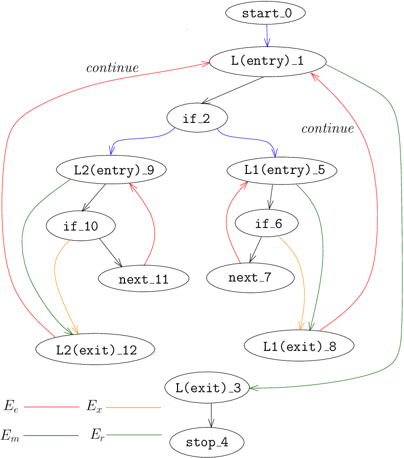
Algorithm 1 (Construct the DAG)
- 1.
Start with . That is and .
- 2.
Remove all backward arcs. Thus, let be all backward edges of ; recall that each of them connects from a node to , for some loop element . Remove all arcs corresponding to edges in from .
- 3.
Remove all arcs leading to a loop-exit. Thus, let be all edges in such that and for some loop element . Recall that these arcs are attributed to break statements. Remove all arcs corresponding to edges in from .
- 4.
Re-route all arcs leading to a loop-entry. Thus, let be all edges in such that and for some loop element . For each such edge, remove the corresponding edge in and replace it by an arc ). Let be those re-routed arcs. Note that now since we also removed all backward edges.
- 5.
Reverse all arcs surrounding a loop. Thus, let be the edges in of the form for some loop element . For each edge, reverse the corresponding arc in . Let be the resulting arcs.
Note that there is a bijective mapping from the vertices in to the nodes in . For ease of representation, assume that are the vertices of and are the corresponding nodes in . We now fill the bags :
For every vertex , set , where is the loop element such that .
A sample decomposition is shown in Figure 2b. Clearly the construction can be done in linear time and digraph has edges. One easily verifies the following:
Observation 1
For every arc , .
It remains to show that is a valid DAG decomposition.
- 1.
is a DAG. We claim that is acyclic. For if it contained a directed cycle , then let be a loop element with , but for any loop element nested under . Therefore contains a vertex of . By Corollary 1 then belongs to , so contains a backward edge. This is impossible since we delete the backward edges.
Adding arcs cannot create a cycle since each arc in it is a shortcut for the 2-edge path from outside to to . In there is no directed path from to , since such a path would reside inside , and the last edge of it belongs to . In consequence adding arcs cannot create a cycle either. Hence is acyclic.
- 2.
Vertices Covered. By definition each is contained in its bag .
- 3.
Connectivity. Let be three nodes in . Recall that their three bags are , and , where are the loop elements to which belong. Nothing is to show unless , which severely restricts the possibilities:
- (a)
Assume first that . Thus and belong to the same loop element, and by the directed path between them, so does . So the claim holds since .
- (b)
If , then the intersection can be non-empty only if (recall that ). But then , and the path from to must go from to to . It follows that also belongs to and so and the condition holds.
- (a)
- 4.
Edges Covered. We only show the second condition; the first one is similar and easier since start is the only source. Let be an arc in . By Observation 1, is the only possible vertex in . Let be an edge of . We have the following cases:
- (a)
If , then and itself can serve as the required successor-bag.
- (b)
If , then . We re-routed as arc and later added an arc , so is a successor of and can serve as the required successor-bag.
- (c)
Finally, if , then is an arc in and is the required successor-bag.
- (a)
We conclude:
Theorem 4.1
Every control-flow graph has a DAG decomposition of width 3 with vertices and edges. It can be found in linear time.
5 Conclusion
In this paper, we showed that control-flow graphs have DAG-width at most . Our proof comes with a linear-time algorithm to find such a DAG decomposition, and it has linear size. Since algorithms that are tailored to small DAG-width are typically exponential in the DAG-width, this should improve the run time of such algorithms for control-flow graphs. The specific application that motivated this paper was the DAG-width based algorithm for parity games from [8]; using our DAG decomposition should turn this into a more practical algorithm for software model checking. (See Appendix 0.C for more details). The run-time is still rather slow for large . One natural open problem is hence to develop even faster algorithms for parity games on digraphs that come from control flow graphs. Our simple DAG-decomposition that is directly derived from the control flow graph might be helpful here.
Our result also opens directions for future research in other related application areas. For example, can we use the small DAG-width of control-flow graphs for faster analysis of the worst-case execution time (which is essentially a variant of the longest-path problem)?
References
- [1] A. V. Aho, R. Sethi, and J. D. Ullman. Compilers: Principles, Techniques, and Tools. Addison-Wesley, Boston, MA, USA, 1986.
- [2] F. E Allen. Control flow analysis. In ACM SIGPLAN Notices, volume 5, pages 1–19. ACM, 1970.
- [3] S. Arnborg, D. G. Corneil, and A. Proskurowski. Complexity of finding embeddings in a k-tree. SIAM J. Algebraic Discrete Methods, 8(2):277–284, 1987.
- [4] D. Berwanger, A. Dawar, P. Hunter, and S. Kreutzer. DAG-Width and parity games. In STACS 2006, volume 3884 of LNCS, pages 524–536. Springer, 2006.
- [5] D. Berwanger, A. Dawar, P. Hunter, S. Kreutzer, and J. Obdržálek. The DAG-width of directed graphs. Journal of Combinatorial Theory, Series B, 102(4):900–923, 2012.
- [6] M. Bojanczyk, C. Dittmann, and S. Kreutzer. Decomposition theorems and model-checking for the modal -calculus. CSL-LICS ’14, pages 17:1–17:10. ACM, 2014.
- [7] E. A. Emerson, C. S. Jutla, and A. P. Sistla. On model checking for the -calculus and its fragments. Theor. Comput. Sci., 258(1-2):491–522, 2001.
- [8] J. Fearnley and S. Schewe. Time and Parallelizability Results for Parity Games with Bounded Tree and DAG Width. Logical Methods in Computer Science, www.lmcs-online.org, 9(2:06):1–31, 2013.
- [9] S. A. Kripke. Semantical Analysis of Modal Logic I. Normal Modal Propositional Calculi. Mathematical Logic Quarterly, 9(5-6):67–96, 1963.
- [10] J. Obdrzálek. Fast mu-calculus model checking when tree-width is bounded. In CAV 2003, volume 2725 of LNCS, pages 80–92. Springer, 2003.
- [11] J. Obdržálek. DAG-width: Connectivity measure for directed graphs. In SODA’06, pages 814–821. ACM-SIAM, 2006.
- [12] P. Hlinený R. Ganian, J. Kneis, A. Langer, J. Obdrzálek, and P. Rossmanith. Digraph Width Measures in Parameterized Algorithmics. Discrete Applied Mathematics, 168:88–107, 2014.
- [13] N. Robertson and P. D. Seymour. Graph minors. II. Algorithmic aspects of tree-width. J. Algorithms, 7(3):309–322, 1986.
- [14] P. D Seymour and R. Thomas. Graph searching and a min-max theorem for tree-width. Journal of Combinatorial Theory, Series B, 58(1):22–33, 1993.
- [15] C. Stirling. Modal and Temporal Properties of Processes. Springer-Verlag, New York, NY, USA, 2001.
- [16] M. Thorup. All structured programs have small tree width and good register allocation. Information and Computation, 142(2):159–181, 1998.
Appendix 0.A Additional Examples
Example 1
We will refer to the vertices by their indices. Suppose that the initial position of the robber is vertex , and the robber plays a lazy strategy, that is, he stays where he is unless a cop comes there, otherwise, he moves to the closest cop-free vertex. Then, the following two sequences of positions are possible. Note that the labels on the transitions represent the corresponding steps of the strategy whereas indicates that the cop was not used.
- I.
stop
- II.
stop
Appendix 0.B Properties of DAG-width
We aim to show that our edge-covering condition is equivalent to the one given by Berwanger et al. [5]. We first review their concepts.
Definition 7 (Guarding)
Let be a digraph and . We say that guards if, for all , if then .
The original edge-covering condition was the following:
(D3) For all edges , guards , where stands for . For any source , is guarded by .
For easier comparison we re-state here our edge-covering condition:
(3a) For any edge in , any vertex , and any edge in , there exists a successor-bag of that contains .
(3b) For source in , any vertex , and any edge in , there exists a successor-bag of that contains .
We will only show that the first half of (D3) is equivalent to (3a); one can similarly show that the second half of (D3) is equivalent to (3b). We first re-phrase (D3) partially by switching to our notation, and partially by inserting the definition of guarding; clearly (D3’) is equivalent to the first half of (D3).
(D3’) For any edge in , any vertex and any edge in , we have .
But , so we can immediately simplify this again to the following equivalent:
(D3”) For any edge in , any vertex and any edge in , we have .
At the other end, we can also simplify (3a), since we now have the shortcut for vertices in a successor-bag of .
(3a’) For any edge in , any vertex , and any edge in , we have .
Thus (D3”) and (3a’) state nearly the same thing, except that for (D3”) the claim must hold for significantly more vertices . As such, (D3”)(3a’) is trivial since .
For the other direction, we need to work a little harder. Assume (3a’) holds. To show (D3”), fix one such choice of edge in and in with . We show that using induction one the number of successors of in . If there are none, then and (D3”) holds since (3a’) does. Likewise (D3”) holds if since (3a’) holds. This leaves the case where . Thus belongs to some strict successor bag of , and hence there exists an arc with . Node has fewer successors than , and so by induction (D3”) holds for edge . We know and , so . So applying (D3”) we know and hence (D3”) also holds for edge .
Appendix 0.C Application to Software Model Checking
In this section we will discuss how exactly the DAG-width based algorithm from [8] for solving parity games is used for software model checking (which is essentially the -calculus model checking problem on control-flow graphs). We start with briefly discussing the modal -calculus, parity games and how to convert the -calculus model checking problem to the problem of finding a winner in parity games.
0.C.1 Parity Game
A parity game consists of a directed graph called game graph and a parity function (called priority) that assigns a natural number to every vertex of .
The game is played between two players and who move a shared token along the edges of the graph . The vertices and are assumed to be owned by and respectively. If the token is currently on a vertex in (for ), then player gets to move the token, and moves it to a successor of his choice. This results in a possibly infinite sequence of vertices called play. If the play is finite, the player who is unable to move loses the game. If the play is infinite, wins the game if the largest occurring priority is even, otherwise wins.
A solution for the parity game is a partitioning of into and , which are respectively the vertices from which and have a winning strategy. Clearly, and should be disjoint.
0.C.2 Modal -calculus
The modal -calculus (see [15] for a good introduction) is a fixed-point logic comprising a set of formulas defined by the following syntax:
Here, is the set of propositional variables, and are maximal and minimal fixed-point operators respectively. The alternation depth of a formula is the number of syntactic alternations between the maximal fixed-point operator, , and the minimal fixed-point operator, .
Given a formula , we say that a -calculus formula is a subformula of , if we can obtain from by recursively decomposing as per the above syntax. For example, the formula has four subformulas: , , and . The size of a formula is the number of its subformulas.
0.C.3 -calculus Model Checking to Parity Games
A model is represented as a digraph with the set of states as vertices and the transitions as edges. The -calculus model checking problem consists of testing whether a given modal--calculus formula applies to . As mentioned earlier, given and , there exists a way to construct a parity game instance such that applies if and only if the parity game can be solved. See e.g. [15] 11 1 Alternatively, see pages 20-23: Obdržálek, Jan. Algorithmic analysis of parity games. PhD thesis, University of Edinburgh, 2006 We note the following relevant points of this transformation:
- 1.1.
Let be the set of all subformulas of and be the size of the formula . For every and we create a vertex in . Therefore, .
- 1.2.
For every , let be the set of vertices of . Clearly, . It holds that for any , there is an edge between any two vertices and of only if .
- 1.3.
The number of priorities in is equal to the alternation depth of the formula plus two. That is, for a -calculus formula with no fixed-point operators, the number of priorities is at least .
0.C.4 -calculus Model Checking on Control Flow Graphs
Recall that given a -calculus formula of length and a control-flow graph , we can create a parity game graph with vertices. Now, we can use either of the treewidth or DAG-width based algorithms from [8] for solving the parity game on . We discuss them individually.
Treewidth based algorithm
Recall that this runs in time where is the treewidth of the game graph . Using Thorup’s result [16] we can obtain a tree decomposition of with width at most . This means that each bag of the tree decomposition contains at most vertices. Using Observation 1.2, we can now obtain a tree decomposition for from by replacing every by , for all . Note that the width of will be .
DAG-width based algorithm
This runs in time where is the DAG-width of the game graph and is the number of edges in the DAG decomposition. Using our main result (Theorem 4.1), we can obtain a DAG decomposition of width and . As in the previous case, we can obtain a DAG decomposition of from by replacing every with , for all . Note that this will have width and .
We can see that even for the smallest possible values and , the treewidth based algorithm runs in time. For the same values, the DAG-width based algorithm runs in , which is better unless . Of course the actual run-times may be influenced by the constants hidden behind the asymptotic notations, but it is fair to assume that the DAG-width based algorithm will be faster for most practical scenarios, especially as and increase.