On the Impact of Antenna Topologies for Massive MIMO Systems

We consider a multi-user (MU) massive MIMO downlink (DL) system with $M$ transmit antennas jointly serving a total of $K$ single-antenna users. We assume time division duplex (TDD) operation with uplink (UL) pilots enabling the transmitter to estimate the DL channel. The $M\times K$ channel matrix, $\mathbf{H}$, is given by [14]

$$\mathbf{H}=\mathbf{R}_{\textrm{t}}^{\frac{1}{2}}\mathbf{H}_{\textrm{iid}},$$

(1)

where $\mathbf{H}_{\textrm{iid}}$ is the $M\times K$ independent and identically distributed (i.i.d.) channel matrix with $\mathcal{CN}(0,1)$ entries, accounting for small-scale Rayleigh fading, and $\mathbf{R}_{\textrm{t}}$ is the $M\times M$ spatial correlation matrix. We consider a cross-polarized (x-pol) antenna configuration, with the spatial correlation matrix modeled via [14]

$$\mathbf{R}_{\textrm{t}}=\mathbf{X}_{\textrm{pol}}\odot\mathbf{R},$$

(2)

where the $M\times M$ matrix $\mathbf{R}$ is the co-polarized (co-pol) spatial correlation matrix, $\odot$ represents the Hadamard product and $\mathbf{X}_{\textrm{pol}}$ is the $M\times M$ x-pol matrix given by

$$\mathbf{X}_{\textrm{pol}}=\mathbf{1}_{M/2}\otimes\begin{bmatrix}1&\sqrt{\delta}\\ \sqrt{\delta}&1\end{bmatrix},$$

(3)

where $\mathbf{1}_{M/2}$ is a $\frac{M}{2}\times\frac{M}{2}$ matrix of ones, $\delta$ denotes the cross-correlation between the two antenna elements in the x-pol configuration and $\otimes$ represents the Kronecker product.

We consider a clustered channel model, shown in Figure 1(a), where we show the zenith AOD offset, $\Delta\theta$, of the wavefront relative to the mean zenith AOD of the cluster, $\theta$. In this scenario, the linear antenna array is located on the $z$ axis. Similarly, if the antenna array was positioned on the $y$ axis, Figure 1(a) would describe the offset azimuth AOD, $\Delta\phi$, relative to the mean azimuth AOD of the cluster, $\phi$. The channel model geometry is clarified in Figure 1(b).

When large numbers of antennas are present, antenna topologies should exploit $x,y$ and $z$ dimensions. In Section III, we derive spatial correlation approximations for the two antenna array topologies: URA and cylindrical, depicted in Figures 2(a) and 2(b), respectively. In Figure 2(a), the URA is geometrically positioned on the $y,z$ plane, where adjacent antennas are separated by $d_{1}$ wavelengths on the $z$ axis and $d_{2}$ wavelengths on the $y$ axis. Adjacent antennas of the cylindrical array, in Figure 2(b), are separated by a displacement of $d_{1}$ wavelengths on the $z$ axis and located at a radius of $\rho$ wavelengths from cylinder center, with respect to the $x,y$ plane.

For both antenna topologies, we express the spatial correlation as the Kronecker product of the azimuth and zenith domain correlations [12]

$$\mathbf{R}=\mathbf{R}_{\phi}\otimes\mathbf{R}_{\theta},$$

(4)

and derive the corresponding correlation coefficients independently in Section III. Thus, we consider the URA correlation matrix as the Kronecker product of an $A$-element ULA in the $z$ dimension (zenith domain) and a $B$-element ULA on the $x,y$ plane (azimuth domain), where $M=A\times B$. Likewise, we consider the cylindrical array correlation as the Kronecker product of an $A$-element ULA in the $z$ dimension and a $B$-element UCA on the $x,y$ plane.

The correlation coefficient between the $a$th and $a^{\prime}$th antenna in the zenith domain can then by given by [11]

$$\mathbf{R}_{\theta(a,a^{\prime})}=\int{\textrm{e}^{j[\Theta_{a}(\Delta\theta)-\Theta_{a^{\prime}}(\Delta\theta)]}p_{\Delta\theta}(\Delta\theta)d\Delta\theta},$$

(5)

where $\Theta_{a}(\Delta\theta)$ is the zenith domain phase shift of the $a$th antennas AOD with respect to a reference antenna, $p_{\Delta\theta}(\Delta\theta)$ is the zenith domain AOD offset PDF relative to the mean zenith AOD of the cluster. Likewise, the correlation coefficient between the $b$th and $b^{\prime}$th antenna element in the azimuth domain is

	$\displaystyle\mathbf{R}_{\phi(b,b^{\prime})}$	$\displaystyle=\int{\int{\textrm{e}^{j[\Phi_{b}(\Delta\phi,\Delta\theta)-\Phi_{b^{\prime}}(\Delta\phi,\Delta\theta)]}}}$
		$\displaystyle~~~~~~~~~~~~~~~~~~~\times p_{\Delta\phi}(\Delta\phi)p_{\Delta\theta}(\Delta\theta)d\Delta\phi d\Delta\theta,$		(6)

where $\Phi_{b}(\Delta\phi,\Delta\theta)$ is the azimuth domain phase shift of the $b$th antennas AOD with respect to a reference antenna, $p_{\Delta\phi}(\Delta\phi)$ is the azimuth AOD offset PDF relative to the mean azimuth angle of the cluster. Note, we assume the azimuth and zenith AOD offset PDF are independent, i.e., $p_{\Delta\phi,\Delta\theta}(\Delta\phi,\Delta\theta)=p_{\Delta\phi}(\Delta\phi)p_{\Delta\theta}(\Delta\theta)$.

We model the azimuth and zenith offset AOD PDFs from measured values described by 3GPP [13]. Thus, the azimuth AOD offset, relative to the mean AOD, is modeled as a Wrapped Gaussian PDF, given by [13]

$$p_{\Delta\phi}(\Delta\phi)=\left\{\begin{array}[]{l l}\frac{1}{\sigma_{\Delta\phi}\sqrt{2\pi}}\sum\limits_{i=-\infty}^{\infty}{\textrm{e}^{-\frac{(\Delta\phi+2\pi i)^{2}}{2\sigma_{\Delta\phi}^{2}}}}&\Delta\phi\in[-\pi,\pi)\\ 0&\textrm{otherwise}\end{array}\right.,$$

(7)

where $\sigma_{\Delta\phi}$ is the standard deviation (SD) of $\Delta\phi$. Similarly, the zenith AOD offset, relative to the mean AOD, is modeled by a Laplacian PDF, given by [13]

$$p_{\Delta\theta}(\Delta\theta)=\left\{\begin{array}[]{l l}\frac{\kappa}{\sqrt{2}\sigma_{\Delta\theta}}\textrm{e}^{-\left|\frac{\sqrt{2}\Delta\theta}{\sigma_{\Delta\theta}}\right|}&\Delta\theta\in[-\pi,\pi)\\ 0&\textrm{otherwise}\end{array}\right.,$$

(8)

where $\sigma_{\Delta\theta}$ is the SD of $\Delta\theta$ and $\kappa=1/(1-\textrm{e}^{-\sqrt{2}\pi/\sigma_{\Delta\theta}})$ normalizes the PDF.

In order to study the effects of antenna topology on the convergence of massive MIMO properties, we consider the convergence metrics used in [8]. We evaluate the convergence of $\mathbf{W}=\frac{1}{M}\mathbf{H}^{\textrm{T}}\mathbf{H}^{\ast}$ by examining a number of well known properties of $\mathbf{W}$ and a deviation matrix $\mathbf{E}=\mathbf{W}-\mathbf{I}_{K}$, where $\mathbf{I}_{K}$ is the $K\times K$ identity matrix. Letting $\lambda_{1},\lambda_{2},\ldots,\lambda_{K}$ denote the eigenvalues of $\mathbf{W}$, we consider: $\lambda$ range, Mean Absolute Deviation (MAD) and Diagonal Dominance, defined respectively as

	$\displaystyle\lambda\textrm{ range}$	$\displaystyle=\lambda_{\textrm{max}}(\mathbf{W})-\lambda_{\textrm{min}}(\mathbf{W}),$		(9)
	$\displaystyle\textrm{MAD}(\mathbf{E})$	$\displaystyle=\frac{1}{K^{2}}\sum_{i=1,j=1}^{K}|\mathbf{E}_{ij}|,$		(10)
	Diagonal Dominance	$\displaystyle=\frac{\sum_{i=1}^{K}{\mathbf{W}_{ii}}}{\sum_{i=1}^{K}{\sum_{j=1,j\neq i}^{K}{|\mathbf{W}_{ij}|}}}.$		(11)

These metrics will be evaluated via simulation for a number of system scenarios in Section IV.

We first consider the correlation in the zenith domain, $\mathbf{R}_{\theta}$, of the URA, depicted in Figure 2(a) and geometrically described in Section II-B. The zenith domain phase shift of the departing wavefront from the $a$th antenna element, relative to a reference antenna, can be expressed as [15]

$$\Theta_{a}(\Delta\theta)=kd_{1}a\cos(\theta+\Delta\theta),$$

(12)

where $k$ is the wavenumber. The angle in (12) can be expanded with a first-order Taylor series, while assuming $\Delta\theta\approx 0$, to give

$$\cos(\theta+\Delta\theta)\approx\cos(\theta)-\Delta\theta\sin(\theta).$$

(13)

Since $p_{\Delta\theta}(\Delta\theta)$ is zero outside the range $[-\pi,\pi)$, the PDFs integration can be taken over $[-\infty,+\infty]$. From (5) we then have

		$\displaystyle\mathbf{R}_{\theta(a,a^{\prime})}\approx\int_{-\infty}^{\infty}{\textrm{e}^{jkd_{1}(a-a^{\prime})[\cos(\theta)-\Delta\theta\sin(\theta)]}p_{\Delta\theta}(\Delta\theta)d\Delta\theta}$		(14)
		$\displaystyle=\textrm{e}^{jkd_{1}(a-a^{\prime})\cos(\theta)}\int_{-\infty}^{\infty}{\textrm{e}^{-jkd_{1}(a-a^{\prime})\sin(\theta)\Delta\theta}}$

		$\displaystyle\times\frac{\kappa}{\sqrt{2}\sigma_{\Delta\theta}}\textrm{e}^{-\left|\frac{\sqrt{2}\Delta\theta}{\sigma_{\Delta\theta}}\right|}d\Delta\theta$		(15)
		$\displaystyle=\textrm{e}^{jkd_{1}(a-a^{\prime})\cos(\theta)}\mathcal{F}_{\omega}\left\{\frac{\kappa}{\sqrt{2}\sigma_{\Delta\theta}}\textrm{e}^{-\left|\frac{\sqrt{2}\Delta\theta}{\sigma_{\Delta\theta}}\right|}\right\},$		(16)

where $\mathcal{F}_{\omega}$ denotes the Fourier transform evaluated at $\omega=kd_{1}(a-a^{\prime})\sin(\theta)$. Solving the Fourier transform in (16), we have the approximation of the correlation coefficient for the zenith domain of a URA as

$\displaystyle\mathbf{R}_{\theta(a,a^{\prime})}\approx\frac{\kappa\textrm{e}^{jkd_{1}(a-a^{\prime})\cos(\theta)}}{1+\frac{\sigma_{\Delta\theta}^{2}}{2}[kd_{1}(a-a^{\prime})\sin(\theta)]^{2}}.$

(17)

We now consider the correlation in the azimuth domain. The azimuth domain phase shift of the departing wavefront from the $b$th antenna element, relative to a reference antenna, can be expressed as [15]

$$\Phi_{b}(\Delta\phi,\Delta\theta)=kd_{2}b\cos(\phi+\Delta\phi)\sin(\theta+\Delta\theta).$$

(18)

We can then use a first-order Taylor series expansion, while assuming $\Delta\phi\approx 0$, to express (18) as

$$\cos(\phi+\Delta\phi)\sin(\theta+\Delta\theta)\approx\sin(\theta+\Delta\theta)\left[\cos(\phi)-\Delta\phi\sin(\phi)\right].$$

(19)

Since both $p_{\Delta\phi}(\Delta\phi)$ and $p_{\Delta\theta}(\Delta\theta)$ are zero outside the range $[-\pi,\pi)$, the integration can be taken over $[-\infty,+\infty]$. From (6), the correlation coefficient between two antenna elements $b$ and $b^{\prime}$ is then given by

$\displaystyle\mathbf{R}_{\phi(b,b^{\prime})}\approx\int_{\infty}^{\infty}{\textrm{e}^{jkd_{2}(b-b^{\prime})\sin(\theta+\Delta\theta)\cos(\phi)}}$

		$\displaystyle\times\left[\int_{-\infty}^{\infty}{\textrm{e}^{-jkd_{2}(b-b^{\prime})\sin(\theta+\Delta\theta)\sin(\phi)\Delta\phi}p_{\Delta\phi}(\Delta\phi)d\Delta\phi}\right]$
		$\displaystyle~~~~~~~~~~~~~~~~~~~~~~~~~~~~~~~~~~~~~~~~~~~~\times p_{\Delta\theta}(\Delta\theta)d\Delta\theta.$		(20)

Considering the integral with respect to $\Delta\phi$, embedded in (20), we have

		$\displaystyle\int_{-\infty}^{\infty}{\textrm{e}^{-jkd_{2}(b-b^{\prime})\sin(\theta+\Delta\theta)\sin(\phi)\Delta\phi}p_{\Delta\phi}(\Delta\phi)d\Delta\phi}$
		$\displaystyle=\int_{-\infty}^{\infty}{\textrm{e}^{-jkd_{2}(b-b^{\prime})\sin(\theta+\Delta\theta)\sin(\phi)\Delta\phi}}$
		$\displaystyle~~~~~~~~~~~~~~~~~~~~~~~\times\sum_{i=-\infty}^{\infty}{\frac{1}{\sigma_{\Delta\phi}\sqrt{2\pi}}\textrm{e}^{-\frac{(\Delta\phi+2\pi i)^{2}}{2\sigma_{\Delta\phi}^{2}}}}d\Delta\phi$		(21)
		$\displaystyle=\mathcal{F}_{\omega}\left\{\sum_{i=-\infty}^{\infty}{\frac{1}{\sigma_{\Delta\phi}\sqrt{2\pi}}\textrm{e}^{-\frac{(\Delta\phi+2\pi i)^{2}}{2\sigma_{\Delta\phi}^{2}}}}\right\},$		(22)

where the Fourier transform in (22) is evaluated at $\omega=kd_{2}(b-b^{\prime})\sin(\theta+\Delta\theta)\sin(\phi)$. Evaluating the Fourier transform, one obtains

		$\displaystyle\mathbf{R}_{\phi(b,b^{\prime})}\approx\textrm{e}^{jkd_{2}(b-b^{\prime})\sin(\theta)\cos(\phi)}\frac{\kappa}{\sqrt{2}\sigma_{\Delta\theta}}$
		$\displaystyle\times\sum_{i=-\infty}^{\infty}{\textrm{e}^{\frac{-1}{2(1-j2\pi i)}\left[\sigma_{\Delta\phi}kd_{2}(b-b^{\prime})\sin(\theta)\sin(\phi)\right]^{2}}}$

$\displaystyle~~~~~\times\mathcal{F}_{\omega}\left\{\textrm{e}^{\frac{-1}{2(1-j2\pi i)}\left[\sigma_{\Delta\phi}kd_{2}(b-b^{\prime})\cos(\theta)\sin(\phi)\right]^{2}(\Delta\theta)^{2}}\right\},$

(23)

where steps from (22) to (23) are given in the Appendix and the Fourier transform in (23) is evaluated at

$$\omega=\left\{\begin{array}[]{rcl}C_{i}-\frac{\sqrt{2}}{\sigma_{\Delta\theta}}&\mbox{for}&\Delta\theta\geq 0\\ C_{i}+\frac{\sqrt{2}}{\sigma_{\Delta\theta}}&\mbox{for}&\Delta\theta<0\end{array}\right.,$$

(24)

where

		$\displaystyle C_{i}=jkd_{2}(b-b^{\prime})\cos(\theta)$
		$\displaystyle\times\left[\cos(\phi)-\frac{1}{j+2\pi i}\sigma_{\Delta\phi}^{2}kd_{2}(b-b^{\prime})\sin^{2}(\phi)\sin(\theta)\right].$		(25)

Evaluating the Fourier transform in (23), we have the approximation of the correlation coefficient for the azimuth domain of a URA as

		$\displaystyle\mathbf{R}_{\Delta\phi(b,b^{\prime})}\approx\frac{\kappa}{\sqrt{2}\sigma_{\Delta\theta}}\textrm{e}^{jkd_{2}(b-b^{\prime})\sin(\theta)\cos(\phi)}$
		$\displaystyle\times\sum_{i=-\infty}^{\infty}{\textrm{e}^{\frac{-1}{2(1-j2\pi i)}\left[\sigma_{\Delta\phi}kd_{2}(b-b^{\prime})\sin(\theta)\sin(\phi)\right]^{2}}}$
		$\displaystyle~~~~~~~~~~~~~~~~~~~~~~~~\times\textrm{e}^{\frac{-\omega^{2}}{\frac{2}{1-j2\pi i}\left[\sigma_{\Delta\phi}kd_{2}(b-b^{\prime})\cos(\theta)\sin(\phi)\right]^{2}}},$		(26)

with $\omega$ given in (24). The spatial correlation approximation for the URA is then as per (4), with $\mathbf{R}_{\theta}$ and $\mathbf{R}_{\phi}$ given in (17) and (26) respectively.

Similar to the analysis for URA, the spatial correlation of a cylindrical array, shown in Figure 2(b), can be broken down into the Kronecker product of the azimuth and zenith domains, described in Section II-B. The zenith domain phase shift of the $a$th antenna element, $\Theta_{a}(\Delta\theta)$, and the correlation coefficient between antennas $a$ and $a^{\prime}$, $\mathbf{R}_{\theta}(a,a^{\prime})$, are identical to the URA case and are thus given in (12) and (17) respectively. In the azimuth domain, the phase shift of the $b$th antenna element, relative to a reference antenna is given by [15]

$$\Phi_{b}(\Delta\phi,\Delta\theta)=k\rho b\cos((\phi-\phi_{b})+\Delta\phi)\sin(\theta+\Delta\theta),$$

(27)

where $\phi-\phi_{b}$ is the angle between the incident ray projected onto the $x,y$ plane and the $b$th antenna, relative to the the circle center. Note that the azimuth domain phase shift in (27) is analogous to (18), with $\rho=d_{2}$ and $\phi-\phi_{b}=\phi$. Therefore, the spatial correlation approximation for the cylindrical array is given in (4), where

		$\displaystyle\mathbf{R}_{\phi(b,b^{\prime})}\approx\frac{\kappa}{\sqrt{2}\sigma_{\Delta\theta}}\textrm{e}^{jk\rho(b-b^{\prime})\sin(\theta)\cos(\phi-\phi_{b})}$
		$\displaystyle\times\sum_{i=-\infty}^{\infty}{\textrm{e}^{\frac{-1}{2(1-j2\pi i)}\left[\sigma_{\Delta\phi}k\rho(b-b^{\prime})\sin(\theta)\sin(\phi-\phi_{b})\right]^{2}}}$
		$\displaystyle~~~~~~~~~~~~~~~~~~~~~\times\textrm{e}^{\frac{-\omega^{2}}{\frac{2}{1-j2\pi i}\left[\sigma_{\Delta\phi}k\rho(b-b^{\prime})\cos(\theta)\sin(\phi-\phi_{b})\right]^{2}}},$		(28)

where $\omega$ is given in (24), with

$\displaystyle C_{i}=jk\rho(b-b^{\prime})\cos(\theta)~\times$

$\displaystyle\left[\cos(\phi-\phi_{b})-\frac{1}{j+2\pi i}\sigma_{\Delta\phi}^{2}k\rho(b-b^{\prime})\sin^{2}(\phi-\phi_{b})\sin(\theta)\right],$

(29)

and $\mathbf{R}_{\theta}$ is given in (17).

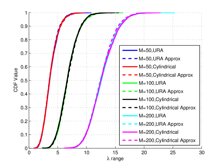
In Figure 3, we show the cumulative distribution function (CDF) of the $\lambda$ range, given in (9), for varying $M$. The eigenvalues of $\mathbf{W}$ are generated using $\mathbf{H}$, given in (1), where the simulated CDFs are generated from instantaneous array factors, while the approximations are generated from (4). It is seen that as we increase the number of transmit antennas, $M$, the median value of the $\lambda$ range CDF increases, rather than converging to an equal eigenvalued channel, which is observed in [8] and shown in [7] for an i.i.d. channel. This is due to an increase in the dominant eigenvalue of $\mathbf{W}$, resulting from such a narrow angle spread. From Figure 3, we see that for all values of $M$, our derived expressions approximate the spatial correlation well. Thus, we use the approximations for all results following.

In Figure 4 we plot the average of MAD($\mathbf{E}$), given in (10), versus $K$ for $\alpha=10$ and $25$. We observe very different behaviour between the correlated and i.i.d. scenarios. In the i.i.d. case, MAD($\mathbf{E}$) converges slowly to zero for increasing $K$, with a quicker convergence rate for larger $\alpha$. Note that the average MAD($\mathbf{E}$) value is plotted in Figure 4 and the only way for this to converge to zero is for all $\mathbf{W}$ matrices to be close to $\mathbf{I}_{K}$. Hence, only in the i.i.d. case does each $\mathbf{W}$ become close to $\mathbf{I}_{K}$ as $K$ increases.

Figure 5 shows the diagonal dominance of $\mathbf{W}$ (size $K\times K$) given in (11), as a function of the number of transmit antennas, $M$. We see that the correlated scenario has similar trends as the i.i.d. case. As with the results in [8] for $K=\frac{M}{\alpha}$, the diagonal dominance decays. This follows as the number of off-diagonals, which grow at a rate $\approx K^{2}$, increase the denominator of (11) at a faster rate than the numerator. In the correlated scenario, the diagonal dominance approaches zero much faster than the i.i.d. case. Here, while the diagonal elements converge to a mean of 1, the large number of off-diagonals converge to a non-zero mean, dominating the diagonal elements. On the other hand, for fixed $K$, the sum of the diagonal elements increase by a greater proportion than the off-diagonal elements as $M$ is increased, resulting in a more diagonally dominant i.i.d. $\mathbf{W}$. In the correlated case the diagonal dominance converges quickly to small non-zero value.

Considering Figures 3, 4 and 5, we conclude that while for i.i.d. channels, the massive MIMO metrics converge for a very large numbers of antennas, desirable massive MIMO properties are degraded with spatial correlation present (with small angle spreads).

We now explore the impact of massive MIMO antenna topologies on MF SINR performance and convergence to limiting values. The MF SINR of the $i$th user is given by

$$\textrm{SINR}_{i}=\frac{\frac{\rho_{\textrm{d}}}{K\gamma}|\mathbf{h}_{i}^{\textrm{T}}\mathbf{h}_{i}^{\ast}|^{2}}{1+\frac{\rho_{\textrm{d}}}{K\gamma}\sum_{j=1,j\neq i}^{K}{\mathbf{h}_{i}^{\textrm{T}}\mathbf{h}_{j}^{\ast}\mathbf{h}_{j}^{\textrm{T}}\mathbf{h}_{i}^{\ast}}},$$

(30)

where $\rho_{\textrm{d}}$ is the DL transmit signal to noise ratio (SNR), $\mathbf{h}_{i}$ denotes the $i$th column of $\mathbf{H}$, and $\gamma=\textrm{tr}(\mathbf{H}^{\textrm{T}}\mathbf{H}^{\ast})/K$ is the power normalization factor.

In Figure 6 we plot the expected value of (30). It can be observed that there is a huge reduction in $\mathbb{E}[\textrm{SINR}_{i}]$ performance by introducing correlation of which antenna topology has almost no effect on. The MF SINR for an i.i.d. scenario rapidly converges to its limiting value, whereas in a correlated case, $\mathbb{E}[\textrm{SINR}_{i}]$ converges to limiting values for $M>200$. We conclude that linear precoders are highly sub-optimal for massive MIMO systems in spatially correlated environments with small angle spreads.

References

- [1] J. Hoydis, K. Hosseini, S. ten Brink, and M. Debbah, “Making smart use of excess antennas: Massive MIMO, small cells, and TDD,” Bell Labs Technical Journal, vol. 18, pp. 5–21, September 2013.
- [2] B. Li and P. Liang, “Small cell in-band wireless backhaul in massive MIMO systems: A cooperation of next-generation techniques,” Bell Labs Technical Journal, February 2014.
- [3] E. Bjornson, M. Kountouris, and M. Debbah, “Massive MIMO and small cells: Improving energy efficiency by optimal soft-cell coordination,” Proceedings of ICT, May 2013.
- [4] T. L. Marzetta, “Noncooperative cellular wireless with unlimited numbers of base station antennas,” IEEE Trans. Wireless Commun., vol. 9, no. 11, pp. 3590–3600, November 2010.
- [5] H. Q. Ngo and E. G. L. anf T. L. Marzetta, “Energy and spectral efficiency of very large multiuser MIMO systems,” IEEE Trans. Commun., vol. 61, no. 4, pp. 1436–1149, April 2013.
- [6] J. Hoydis, S. ten Brink, and M. Debbah, “Massive MIMO in the UL/DL of cellular networks: How many antennas do we need?” IEEE J. Sel. Areas Commun., vol. 31, no. 2, pp. 160–171, February 2013.
- [7] F. Rusek, D. Persson, B. K. Lau, E. G. Larsson, T. L. Marzetta, O. Edfors, and F. Tufvesson, “Scaling up MIMO: Opportunities and challenges with very large arrays,” IEEE Signal Process. Mag., vol. 30, no. 1, pp. 40–60, January 2013.
- [8] P. J. Smith, C. T. Neil, M. Shafi, and P. A. Dmochowski, “On the convergence of massive MIMO systems,” IEEE Int. Conf. Commun. (ICC), June 2014.
- [9] X. Gao, O. Edfors, F. Rusek, and F. Tufvesson, “Massive MIMO in real propagation environments,” IEEE Trans. Wireless Commun., March 2014.
- [10] D.-S. Shiu, G. J. Foschini, M. J. Gans, and J. M. Kahn, “Fading correlation and its effect on the capacity of multielement antenna systems,” IEEE Trans. Commun., vol. 48, no. 3, pp. 502–513, March 2000.
- [11] A. Forenza, D. J. Love, and R. W. H. Jr, “Simplified spatial correlation models for clustered MIMO channels with different array configurations,” IEEE Trans. Veh. Technol., vol. 56, no. 4, pp. 1924–1934, July 2007.
- [12] D. Ying, F. W. Vook, T. A. Thomas, D. J. Love, and A. Ghosh, “Kronecker product correlation model and limited feedback codebook design in a 3D channel model,” IEEE Int. Conf. Commun. (ICC), pp. 5876–5881, June 2014.
- [13] “Study on 3D channel model for LTE (release 12),” 3rd Generation Partnership Project; Technical Specification Group Radio Access Network, vol. V2.0.0, March 2014.
- [14] A. Paulraj, R. Nabar, and D. Gore, Introduction to Space-Time Wireless Communications, 1st ed. Cambridge University Press, 2003.
- [15] C. A. Balanis, Antenna Theory: Analysis and Design, 3rd ed. John Wiley and Sons, 2005.
- [16] Alcatel-Lucent New Zealand Limited, “MIMO channel measurement campaign: Phase 1,” vol. 1.2, pp. 59–101, September 2009.