Quantum field theory in a magnetic field:
From quantum chromodynamics to graphene and Dirac semimetals
Abstract
A range of quantum field theoretical phenomena driven by external magnetic fields and their applications in relativistic systems and quasirelativistic condensed matter ones, such as graphene and Dirac/Weyl semimetals, are reviewed. We start by introducing the underlying physics of the magnetic catalysis. The dimensional reduction of the low-energy dynamics of relativistic fermions in an external magnetic field is explained and its role in catalyzing spontaneous symmetry breaking is emphasized. The general theoretical consideration is supplemented by the analysis of the magnetic catalysis in quantum electrodynamics, chromodynamics and quasirelativistic models relevant for condensed matter physics. By generalizing the ideas of the magnetic catalysis to the case of nonzero density and temperature, we argue that other interesting phenomena take place. The chiral magnetic and chiral separation effects are perhaps the most interesting among them. In addition to the general discussion of the physics underlying chiral magnetic and separation effects, we also review their possible phenomenological implications in heavy-ion collisions and compact stars. We also discuss the application of the magnetic catalysis ideas for the description of the quantum Hall effect in monolayer and bilayer graphene, and conclude that the generalized magnetic catalysis, including both the magnetic catalysis condensates and the quantum Hall ferromagnetic ones, lies at the basis of this phenomenon. We also consider how an external magnetic field affects the underlying physics in a class of three-dimensional quasirelativistic condensed matter systems, Dirac semimetals. While at sufficiently low temperatures and zero density of charge carriers, such semimetals are expected to reveal the regime of the magnetic catalysis, the regime of Weyl semimetals with chiral asymmetry is realized at nonzero density. Finally, we discuss the interplay between relativistic quantum field theories (including quantum electrodynamics and quantum chromodynamics) in a magnetic field and noncommutative field theories, which leads to a new type of the latter, nonlocal noncommutative field theories.
Keywords:
magnetic catalysis, spontaneous symmetry breaking, relativistic matter, chiral asymmetry, graphene, Dirac semimetals1 Introduction
The gravitational and electromagnetic forces are the only known long-range interactions in Nature. Because of this property, they lead to numerous easily observed macroscopic phenomena and become an integral part of our everyday life. This is also the main reason why these two forces were discovered long time ago. Systematic studies of the gravitational forces with the use of modern scientific methods started in the 16th-17th centuries (with the works of Galileo Galilei, Isaac Newton and others), and the studies of electromagnetism began in the 19th century (with the works of Alessandro Volta, Hans Christian Oersted, Andre-Marie Ampere, Michael Faraday, and James Clerk Maxwell, and many others). The other two known fundamental interactions of nature, responsible for the strong and weak forces, are short range and can be detected only under very special laboratory conditions. They were discovered much later, in the middle of the 20th century.
It is not surprising, therefore, that the first two classical field theories were the theory of electromagnetism (the Maxwell’s theory) and the theory of gravity (the Newton’s law of universal gravitation and later the Einstein’s theory of general relativity). The Maxwell’s theory led to remarkable discoveries, one of which was the understanding of the electromagnetic nature of light.
The electromagnetic interactions became even more important in the quantum epoch, when the quantum nature of numerous phenomena was revealed. The paramagnetism of metals was described by the Pauli theory [1, 2], the diamagnetism was described by the Landau theory [3], and the ferromagnetism found the explanation in the Heisenberg theory [4]. New effects, such as the Meissner effect in superconductivity [5], Shubnikov-de Haas effect (oscillations) [6, 7, 8] in metals and semimetals, quantum Hall effect [9, 10, 11] in semiconductors, to name few, were discovered.
With the development of quantum field theory, a whole range of other quantum phenomena was discovered and explained theoretically. Of particular importance among them was the Bardeen-Cooper-Schrieffer (BCS) theory of low-temperature superconductivity [12, 13]. In addition to being of great value on its own, it inspired numerous applications of spontaneous (dynamical) symmetry breaking mechanisms to various subfields of physics. In particle physics, for example, the mechanism of symmetry breaking helped to understand the puzzling low-energy spectrum of QCD, allowed a natural unification of the electromagnetic and weak interactions, and gave a real hope for the ultimate unification of all forces in Nature. The success of the corresponding ideas also shaped our understanding of cosmology. In particular, they implied that symmetry breaking phase transitions should have occurred during the evolution of the early Universe. Considering the likely existence of very strong magnetic fields at that epoch [14, 15, 16, 17, 18, 19], it is natural to ask how the underlying dynamics and the phase transition were affected by such fields. Can one utilize the longtime experience from low-temperature superconductivity to answer the question? In general, the answer is “No".
As is well known, in low-temperature superconductors, an external magnetic field has a tendency to break superconductivity by interfering with Cooper pairing. At the microscopic level, this can be understood as the result of interaction of the electrons’ magnetic moments with the field. The seemingly favorable alignment of the magnetic moments with the direction of the magnetic field comes in a direct conflict with the antiparallel alignment inside Cooper pairs. However, this example alone does not help to shed light on the underlying dynamics in relativistic systems undergoing other types of phase transitions, associated with spontaneous (dynamical) symmetry breaking. In fact, as we discuss in this review, there exist (quasi-)relativistic systems, in which external magnetic fields not only enhance, but even induce symmetry breaking.
Here it may be appropriate to emphasize that magnetic fields indeed play an important role in the dynamics of many relativistic and quasirelativistic systems. These range from the already mentioned evolution of the early Universe to the fireballs of quark-gluon plasma created in heavy-ion collisions, from compact stars to numerous condensed matter systems. The latter, in particular, include a growing number of quasirelativistic systems, such as 2-dimensional graphene and a number of 3-dimensional Dirac (semi-)metals. It is also hoped that, by making use of certain topological properties of materials and crystal symmetries, other types of quasirelativistic materials will be possible to engineer in the future. One of such exotic possibilities is Weyl semimetals.
The origin of the magnetic field may differ from one system to another. In some cases, one may simply apply external (electro-)magnetic fields in order to either probe its physical properties, or to better understand the underlying physics. In other cases, the production of the magnetic field is the native property of the system. In heavy-ion collisions, for example, very strong magnetic fields are generated during the early stages of the collisions as the result of the electric currents from the colliding positively charges ions [20, 21, 22, 23, 24, 25]. Because of the high electric conductivity of the medium, the corresponding fields may survive for as long as the lifetime of the quark-gluon plasma itself and, thus, have a profound effect on its dynamics. In the case of the early Universe, several competing mechanisms responsible for the generation of very strong magnetic fields were proposed [14, 15, 16, 17, 18, 19]. Despite the differences in the details, the consensus is that rather strong fields should have been generated. This is required by the present day observations of weak, but nonvanishing intergalactic magnetic fields. In the case of compact stars, the existence of strong magnetic fields is inferred from the observational data [26, 27, 28], even though the exact nature of the underlying mechanism [29, 30] responsible for generation of such fields may still be debated. It is clear, however, that such fields exist and play a profound role in the stellar physics.
With the discovery of quasirelativistic condensed matter systems such as graphene [31], it became clear that a whole new realm of interesting quantum phenomena induced by a magnetic field can be realized in simple table-top experiments. In fact, the experimental proof that the low-energy excitations in graphene are Dirac quasiparticles was obtained by analyzing the observational features of the quantum Hall effect in a weak field [32, 33]. In a strong magnetic field, on the other hand, a number of additional quantum Hall states were observed. It can be argued that such states are the consequence of a series of symmetry breaking quantum phase transitions, induced by the external field.
In this review, we will describe in detail the role of the magnetic field in a number of (quasi-)relativistic systems, using the results derived by analytic quantum field theoretical methods. In particular, we will try to place the emphasis on the underlying physics. When possible, the theoretical results will be compared with lattice simulations of the magnetic field induced dynamics in quantum chromodynamics and in graphene. In the case of graphene, we will also make a comparison of theoretical predictions with the experimental data.
We will start the review by introducing the underlying physics of the magnetic catalysis phenomenon [34, 35, 36]. We will discuss in detail the origin of the dimensional reduction in low-energy theories describing the interactions of charged relativistic fermions in an external magnetic field, the implication of such dimensional reduction for the particle-antiparticle pairing dynamics and the spontaneous (dynamical) symmetry breaking associated with it. Finally, we will make the case about the universality of the underlying mechanism. The general theoretical considerations will be followed by the discussion of applications of the magnetic catalysis in quantum electrodynamics (QED), quantum chromodynamics (QCD), and other relativistic models. We will also discuss the magnetic catalysis phenomenon in a class of quasirelativistic systems, such as highly oriented pyrolytic graphite, monolayer and bilayer graphene.
By generalizing the ideas of the magnetic catalysis to the case of nonzero density and temperature, we will show that other interesting phenomena are realized in various types of relativistic matter. The chiral magnetic effect [37, 21, 38] and the chiral separation effect [14, 39, 40] are the two important examples of such phenomena that take place at nonzero density. We will present recent theoretical ideas about these two effects and their possible phenomenological implications in heavy-ion collisions and in compact stars. We will also discuss condensed matter analogues of these phenomena. In particular, we will argue about an interesting possibility of dynamical transformation of Dirac semimetals into Weyl ones, and suggest possible experimental signatures associated with such a transformation.
It is worth noting that the studies of relativistic quantum field theories in magnetic fields have a long history starting from the classic papers by Heisenberg and Euler [41], and Schwinger [42] (for an excellent historical review of these papers, see Ref. [43]). A lot of theoretical progress in this area has been achieved since then, especially in connection to theories with spontaneous symmetry breaking, in which external fields may play a profound role in the underlying dynamics. Currently, however, there exist no comprehensive reviews on the topic. We hope that this review will fill the gap at least partly.
2 Magnetic catalysis
The fact that an external magnetic field enhances the generation of a fermion mass in dimensions was first established in the framework of the Nambu–Jona-Lasinio (NJL) model in Refs. [44, 45]. Also, in the context of the -dimensional Gross-Neveu model, which was expected to give a simple effective description for certain condensed matter planar systems, the authors of Refs. [46, 47, 48, 49] showed that the dynamical generation of a nonzero fermion mass takes place in a magnetic field as soon as there is an attractive interaction between fermions and antifermions. It will be fair to say, however, that the underlying mechanism in these early studies remained mysterious.
Most of the early model calculations did not address the underlying reason for the puzzling role of an external magnetic field as a trigger of symmetry breaking. To put this in perspective, one should recall that, at the time, the standard source of physics intuition for many nuclear and particle physics models with dynamical symmetry breaking was the BCS theory of superconductivity. By all accounts, however, the results of the NJL model revealed a drastically different role of the magnetic field. It helped to break, rather than restore symmetry. Also, there was no perfect diamagnetism and no Meissner effect associated with the broken phase.
Perhaps one exception from the general rule was the review of the NJL model by Klevansky [50], which indeed offered a general qualitative explanation why an electric field tends to restore chiral symmetry and the magnetic field tends to break it. The reasoning went as follows: “the electric field destroys the condensate by pulling the pairs apart, while the magnetic field aids in antialigning the helicities which are bound by the NJL interaction." Also, there it was clarified that the “surprising" response to the magnetic field was so different from that in the theory of superconductivity because the pairing in the NJL model was between particles and antiparticles that carry opposite charges. This is in contrast to the usual Cooper pairing, which involves particles of the same charge.
While later it was found that there is much more to it, such an explanation was the first step in establishing the underlying physics of the magnetic catalysis. Also, as we will demonstrate in this section, despite the obvious differences pointed above, there are in fact profound, although more subtle, similarities between the dynamics of the magnetic catalysis and superconductivity.
Without a solid understanding of the underlying physics, it is hard to appreciate how important or how general is the mechanism, found in the models with local four-fermion interaction. Will it also work in more realistic gauge models with long-range interaction? What are the similarities and differences between models in various space-time dimensions? Answering these and other related questions is the main goal of this section.
This mystery was resolved and the theoretical basis for the magnetic catalysis in both and dimensions was built in Refs. [34, 35, 36]. It was revealed that the origin of the magnetic catalysis is the dimensional reduction (i.e., and ) in the infrared dynamics of the fermion pairing in a magnetic field. As is well known, in a lower dimension the infrared dynamics become stronger. A classical example of this phenomenon is provided by the Bardeen-Cooper-Schrieffer (BCS) theory of superconductivity [13, 12]. The physical reason of this reduction is the fact that the motion of charged particles is restricted in those directions that are perpendicular to the magnetic field. This is in turn connected with the point that, at weak coupling between fermions, the fermion pairing, leading to the chiral (in general case, flavor) condensate, is mostly provided by fermions from the lowest Landau level (LLL) whose dynamics is -dimensional. The effect was called the magnetic catalysis [34].
Thus, a constant magnetic field in and dimensions is a strong catalyst of dynamical chiral symmetry breaking, leading to the generation of a dynamical fermion mass even at the weakest attractive interaction between fermions and antifermions. It is crucial that the magnetic catalysis effect is universal and takes place for any fermion-antifermion attractive interaction.
The model-independent nature of magnetic catalysis was tested in numerous - and -dimensional models with local four-fermion interactions [34, 35, 36, 51, 52, 53, 54, 55, 56, 57, 58, 59, 60, 61, 62, 63, 64, 65, 66, 67, 68, 69, 70, 71, 72, 73], as well in spatial dimensions [74] and in models with additional gauge interactions [56] and Polyakov loop effects [75, 76, 77, 78, 79, 80, 81, 82], supersymmetric models [83], quark-meson models [84, 85, 86, 87, 88, 89], models in curved space [90, 91, 92, 93]. The realization of magnetic catalysis was investigated in chiral perturbation theory [94, 95, 96, 97, 98, 99, 100] and in models with the Yukawa interaction [101, 102, 103, 104]. The mechanism of the magnetic catalysis is supported by the arguments of the renormalization group [105, 106, 107, 108, 81, 109, 110, 111].
By now, the magnetic catalysis has been extensively studied not only in the NJL model but also in realistic theories, such as quantum electrodynamics (QED) and quantum chromodynamics (QCD) by using both analytic quantum-field theoretical approaches [112, 113, 114, 115, 116, 117, 118, 119, 120, 121, 122, 123, 124, 125, 126, 127, 128, 129, 130, 131, 132, 133, 134, 135], holographic models [136, 137, 138, 139, 140, 141, 142, 143, 144, 145, 146, 147, 148, 149, 150, 151, 152, 153, 154, 155, 156], lattice simulations of -dimensional QED [157, 158, 159, 160, 161] and QCD-like gauge theories [162, 163, 164, 165, 166, 167, 168, 169, 170, 171, 172, 173, 174, 175]. It is also noticeable that the magnetic catalysis is a basic mechanism in the dynamics of the quantum Hall effect in graphene [176, 177, 178, 179, 180, 181, 182] (see Section 4). Ideas inspired by the magnetic catalysis were even extended to solid state systems such as high-temperature superconductors [183, 184, 185, 186, 187, 188] and highly oriented pyrolytic graphite [189, 190, 191]. Finally, the generalization of magnetic catalysis was also made to non-Abelian chromomagnetic fields [192, 193, 194, 195, 196, 197, 198], where the dynamics is dimensionally reduced by one unit of space, .
In this section, we will start from the description of the simplest realization of the magnetic catalysis phenomenon in the NJL models with a large number of fermion colors . We will discuss models in and space-time dimensions, and emphasize the role of the number of dimensions. (The magnetic catalysis effect in gauge theories, including QED and QCD, will be considered in Section 3.) The rest of the section is organized as follows. In Section 2.1, general remarks concerning the magnetic catalysis effect in dimensions are made. In Sections 2.2 and 2.3, we consider the problem of free relativistic fermions in a magnetic field in dimensions. We show that the roots of the fact that a magnetic field is a strong catalyst of dynamical flavor symmetry breaking are already present in this problem. In Section 2.4, we study the NJL model in a magnetic field in dimensions. We derive the low-energy effective action and determine the spectrum of long wavelength collective excitations in the NJL model. We also study the thermodynamic properties of the NJL model in a magnetic field in dimensions. In particular, the phase transitions with respect to temperature and the fermion chemical potential are described. The discussion of the -dimensional free fermions in a magnetic field is presented in Section 2.5, and the analysis of the magnetic catalysis in the NJL model in dimensions is given in Section 2.6. In Section 2.7, the Bethe-Salpeter equations for the Nambu-Goldstone bosons in the NJL model in a magnetic field in both and dimensions are analyzed. The role on magnetic translations is discussed in Section 2.8. In Section 2.9, we summarize the main results in and dimensions.
2.1 Opening remarks
During the past three decades, there has been a considerable interest in studying relativistic field models in dimensions. Not only the rich and sophisticated dynamics in dimensions is interesting from a theoretical viewpoint, the corresponding models also serve as effective theories for the description of long wavelength excitations in a class of planar condensed matter systems. In particular, as will be discussed at length in Section 4, they play an important role for the description of the dynamics in graphene.
In this section, we will show that a constant magnetic field acts as a strong catalyst of dynamical flavor symmetry breaking leading to the generation of fermion masses in dimensions. We will in particular show that there is a striking similarity between the role of the magnetic field in -dimensional models and the role of the Fermi surface in the Bardeen-Cooper-Schrieffer (BCS) theory of superconductivity [13, 12]: both of them enhance the interactions of fermions in the infrared region (at low energies) and, therefore, are responsible for a dynamical generation of a fermion mass (an energy gap in the spectrum) even at the weakest attractive interaction between fermions.
We note that, in absence of a magnetic field, supercritical dynamics (with an effective coupling constant being larger than a critical value ) is a common prerequisite for generating a dynamical fermion mass in and dimensions (for reviews, see Refs. [199, 200, 201]). As will be shown below, in dimensions, a magnetic field reduces the value of the critical coupling to zero. In other words, in a magnetic field, the generation of a fermion mass happens even at the weakest attractive interaction between fermions and antifermions. The essence of this effect is that in a magnetic field, in dimensions, the dynamics of fermion pairing (relating essentially to fermions in the lowest Landau level) is one-dimensional, see Section 2.3.
We stress that this effect is universal (i.e., model independent) in dimensions. This point, in particular, will be important in connection with the use of the magnetic catalysis phenomenon for the description of the quantum Hall effect in graphene, see Section 4. As a soluble example, in this section we will consider the NJL model in a magnetic field, in the leading order in expansion, where is the number of fermion “colors”. Another type of the -dimensional model, which is more relevant for the description of condensed matter systems (in, particular, graphene), will be considered in Section 3.2. It is the reduced QED [202, 203, 189], in which fermions are restricted to a plane and the (electromagnetic) gauge fields propagate in a three-dimensional bulk.
2.2 Free fermions in a magnetic field in dimensions
Before starting a detailed analysis of the dynamics underlying the phenomenon of magnetic catalysis, it is instructive to review the problem of free relativistic fermions in a magnetic field in dimensions. By first introducing a nonzero fermion mass as an infrared regulator in such a theory, and then taking the limit , we will show that the roots of magnetic catalyst of flavor symmetry breaking are already present in the free theory. Indeed, as we will show in Section 2.3.2, the structure of the corresponding ground state bares some resemblance to superfluidity in an almost ideal Bose gas [204].
2.2.1 Two-component spinor representation
In dimensions, the Lagrangian density in the problem of a relativistic fermion in a constant magnetic field takes the following form:
| (1) |
where the space-time position four-vector is denoted by and . According to our convention, the Lorentz indices are denoted by Greek letters (, , , etc.) and run over , , or , , . (In dimensions, another spatial direction, denoted by either or , will be added.) The spatial indices are denoted by Latin letters from the middle of the alphabet (, , , etc.) and run over , or , . The Minkowski metric tensor is given by , and the spatial vectors are identified with the contravariant components of four-vectors. The covariant derivative is defined as usual,
| (2) |
where is the charge of the fermion (e.g., in the case of the electron ). We will assume that the external magnetic field is described by the vector potential in the Landau gauge,
| (3) |
or in the vector notation, . As is easy to check, the corresponding field strength tensor is given by , where . We note that the magnetic field is a pseudoscalar in dimensions.
The Dirac gamma matrices obey the Clifford-Dirac algebra in dimensions, i.e., . This algebra has two inequivalent matrix representations, which can be chosen, for example, as follows:
| Representation I: | (4) | ||||
| Representation II: | (5) |
where are the Pauli matrices.
Let us begin by considering the representation in Eq. (4) and determine the corresponding energy spectrum in the model described by Eq. (1). In the Landau gauge (3), it is convenient to write the general solution in the form , where is a new dimensionless coordinate replacing , and is the magnetic length. Then, the equation of motion for the two-component spinor takes the following form:
| (6) |
For concreteness, let us first assume that and . Then, by solving the eigenvalue problem, we obtain the following energy spectrum [35]:
| (7) | |||||
| (8) |
This energy spectrum describes the Landau levels labeled by a nonnegative integer index . The corresponding eigenstates are given by [205]
where we introduced the following harmonic oscillator wave functions:
| (18) |
which are given in terms of the Hermite polynomials [206]. Note that functions satisfy the following “ladder" identities:
| (19) | |||||
| (20) |
where
| (21) | |||||
| (22) |
are the annihilation and creation operators, respectively. They satisfy the canonical commutation relation . By making use of these operators, in fact, the spectral problem in Eq. (6) can be solved in a symbolic form without the need to explicitly solve any differential equations.
From the above solutions, we see that the Landau levels are highly (infinitely) degenerate. Indeed, their energies depend only on the integer index , but have no dependence on the quantum number . In the Landau gauge used, the latter can be formally interpreted as the momentum associated with the spatial direction . An alternative dual interpretation of , as the center of the fermion orbit in coordinate space, follows from the fact that the corresponding wave functions are localized around , or equivalently around in the spatial direction .
In order to determine the density of states in the Landau levels, we can use the following simple arguments. First, we assume that the system has a finite size, and , in the spatial directions and , respectively. By enforcing the periodic boundary conditions in the direction, we will find that the values of the corresponding momentum are quantized: where . Then, by taking into account that the same momentum also determines the position around which the wave function is localized, we have to require that . In terms of the integer quantum number , the constraint takes the following form: . Therefore, the total number of degenerate states in each Landau level is , and the density of states per unit area is [205].
The general solution for the spinor field is given by
| (23) |
where and are operator-valued coefficients, which can be interpreted as particle annihilation and antiparticle creation operators, respectively.
As is obvious from the general solution, the lowest Landau level with is special. It contains only positive energy states (particles) with . This is in contrast to all higher Landau levels with , which include solutions with both positive energies , describing particle states, and negative energies , describing antiparticle states.
The spectral asymmetry of the lowest Landau level is sensitive to the sign of . To show this, let us write down the general solution for the fermion field in the case of . Instead of solving the spectral equation in Eq. (6) directly, we could use the fact that the two sets of solutions (i.e., for and ) are related by the charge conjugation symmetry, . Therefore, the general solution for the spinor field at can be written in the following form:
| (24) |
where the charge conjugate spinors are defined as follows: and . Note that and are the Dirac conjugate of the eigenfunctions and in Eqs. (2.2.1) – (2.2.1). In this solution, the lowest Landau level with describes negative energy states (antiparticles) with .
It is straightforward to check that, if we use the second representation of the Dirac matrices, given in Eq. (5), the general solution will be given again by an expression like that in Eq. (23), but with the eigenstates and replaced by and , respectively, i.e.,
| (25) |
[The factor is introduced here for convenience.] In this representation, the LLL solutions correspond to antiparticle states with when and particle states with when .
2.2.2 Four-component spinor representation
We note that the mass term in the Lagrangian density (1) violates parity defined by the following transformation of the fermion field:
| (26) |
In order to construct a -dimensional theory of massive Dirac fermions that preserves this discrete symmetry, it is convenient to use the language of four-component fermions [207, 208], connected with a (reducible) four-dimensional representation of the Dirac matrices,
| (27) |
Then, the mass term in the corresponding Lagrangian density
| (28) |
will indeed preserve parity defined by
| (29) |
where the additional Dirac matrix is given by
| (30) |
In the massless limit (), the Lagrangian density (28) is invariant under the global (flavor) symmetry. The corresponding transformations are determined by the following generators:
| (31) |
where
| (32) |
The mass term breaks this symmetry down to the with the generators and .
In the case of the four-component fermions, the energy spectrum is given by
| (33) | |||||
| (34) |
[Compare with Eqs. (7) and (8).] The density of the lowest Landau level () states with the energies is , and it is for higher Landau level states ().
We note that the four-component fermions naturally appear in low-energy effective actions describing planar condensed matter systems with two sublattices, see Section 4. Moreover, usually they appear in the actions without a mass term, and the important problem is to establish a criterion of dynamical flavor symmetry breaking, which may occur as a result of interaction between fermions [201, 209, 210, 211, 212, 213, 214]. As was already indicated in Section 2.3, dynamical flavor symmetry breaking in dimensions usually takes place only at a rather strong effective coupling between fermions.
2.3 Symmetry breaking for free fermions in a magnetic field in dimensions
Let us now show that at and , the dynamical breakdown of the flavor symmetry takes place already in the theory (28), even without any additional interaction between fermions. In order to prove this, we will show that in the limit , there is a nonzero symmetry breaking flavor condensate, .
2.3.1 Nonzero flavor condensate
The condensate can be expressed in terms of the fermion propagator as follows:
| (35) |
The explicit form of the fermion propagator in an external magnetic field, , is given in Eq. (923) in Appendix A in the Schwinger proper-time representation [42]. The result has the form of a product of the Schwinger phase, , and a translation invariant function . In Eq. (925) in the same Appendix, we also present the Fourier transform of the translation invariant part of the propagator. In Euclidean space , the latter takes the following form:
| (36) |
Here , and are antihermitian matrices. [In Euclidean space, the metric tensor coincides with the unit matrix and, therefore, there is no difference between the covariant and contravariant components of vectors.]
In the limit , the Schwinger phase vanishes and, thus, plays no role in the calculation of the condensate defined by Eq. (35). Then, by making use of the translation invariant part of the propagator in Eq. (36), we derive the following result:
| (37) |
where the Gaussian integration over momenta can be performed exactly. In the limit , in particular, the result reads
| (38) | |||||
where an ultraviolet cutoff was used as a regulator at intermediate steps of the calculation. Note that the limit is taken before the limit .
The result in Eq. (38) indicates that, in the presence of a constant magnetic field, spontaneous breakdown of the flavor symmetry takes place even in the free massless theory! This is exclusively a -dimensional phenomenon. Indeed, as we will see later, the corresponding result in dimensions is very different: , which goes to zero as [see Eq. (115)].
What is the physical origin of this phenomenon? In order to answer this question, we note that the singular behavior of the integral in Eq. (38) comes from the infrared region at large values of the proper-time coordinate, . Moreover, one can see from Eq. (38) that the presence of a nonzero magnetic field is responsible for such a behavior. At large values of the proper time, , the function in the integrand approaches a constant value , which is in contrast to in the case of . From the physics viewpoint, this reflects the fact that the magnetic field removes the two perpendicular space dimensions in the low-energy dynamics, making it effectively one-dimensional (in Euclidean space) and, thus, much more singular in infrared.
It can be also argued that the spontaneous breakdown of the flavor symmetry in dimensions is intimately connected with the form of the energy spectrum of fermions in a constant magnetic field. As we see from Eq. (33), in the limit , the energies of all lowest Landau states go to zero and the vacuum becomes infinitely degenerate. It is not coincidental that the value of the condensate (38) is determined by the density of the LLL states per unit area of the system. Also, the effective one-dimensional dynamics behind the flavor symmetry breaking mechanism, mentioned above, finds a simple explanation in the one-dimensional character of the LLL, which is described by a single continuous variable .
This observation suggests that the effect of the magnetic field in the present problem is similar to that of the Fermi surface in the BCS theory of superconductivity [13, 12]. However, as we discuss in Section 2.4.1, there are important differences between them. In particular, the magnetic catalysis effect in dimensions is much stronger than in the BCS theory. [At the same time, as we will see in Section 2.5, there is indeed a close similarity between the dynamics in the BCS theory and the magnetic catalysis in dimensions.]
To make this statement more rigorous mathematically, let us rewrite the fermion propagator in a form of an expansion over Landau levels. The desired form of the propagator can be obtained from Eq. (36) by making use of the following identity and the relation [206]
| (39) |
where are the generalized Laguerre polynomials. The resulting alternative representation of the propagator reads [215]
| (40) |
where
| (41) | |||||
Here and by definition. The expansion over Landau levels in Eq. (40) makes it easy to see that, in the limit , the chiral condensate (38) comes exclusively from the lowest Landau level:
| (42) |
Last but not least, this chiral condensate is equal (up to an overall sign) to the density of the LLL states per unit area in the -plane. Due to the Atiyah-Singer index theorem [216], the latter is a topological invariant. Beyond the zero mass limit, the chiral condensate will also receive contributions from the higher Landau levels and, therefore, will not be topologically protected.
In the next subsection, we will discuss aspects of spontaneous flavor symmetry breaking for ()-dimensional fermions in a magnetic field in more detail.
2.3.2 Haag criteria of spontaneous symmetry breaking
As was shown in the preceding section, the flavor condensate is nonzero as the fermion mass goes to zero. Although usually such a nonvanishing condensate is considered as a firm signature of spontaneous flavor (chiral) symmetry breaking, the following questions may arise in this case:
- (i)
Unlike the conventional spontaneous flavor (chiral) symmetry breaking, the dynamical mass of fermions is vanishing in this problem. Therefore, one may wonder whether there is real symmetry breaking in this case.
- (ii)
The vacuum was defined as from the vacuum in the theory with . Such a vacuum corresponds to a particular filling of the lowest Landau level. Indeed, in the vacuum at , the particle states with are empty and the antiparticle states with are filled. Thus, the vacuum is annihilated by all the operators , and , , , (). On the other hand, at , there is an infinite degeneracy of the vacua, connected with different fillings of the lowest Landau level. Why should one choose the filling leading to the vacuum ? Also, is there a filling of the lowest Landau level leading to the ground state which is invariant under the flavor ? One might think that the latter possibility would imply that spontaneous flavor symmetry breaking can be avoided.
In this section we will show that there is a genuine realization of spontaneous breaking of the flavor symmetry in the present problem. More precisely, we will show that this phenomenon satisfies the Haag criteria of spontaneous symmetry breaking [217]. We will also discuss the status of the Nambu–Goldstone (NG) modes and the induced quantum numbers [218, 219] in the problem at hand.
Let us begin by constructing the charge operators of the flavor group with the generators defined in Eq. (31). By making use of the fermion fields in Eqs. (23) and (25), we derive
| (43) | |||||
| (44) | |||||
| (45) | |||||
| (46) |
where , , (, ) are annihilation operators of fermions (antifermions) from the th Landau level and is the two-dimensional volume. Now we can construct an infinite set of degenerate vacua
| (47) |
where the vacuum is annihilated by all the operators , , , and . As one can see from Eqs. (44) and (45), the crucial point for the existence of the continuum of degenerate vacua is the first sum, over the states in the lowest Landau level, in the definitions of the charges and .
The presence of such a set of degenerate vacua is a signal of the spontaneous breakdown of flavor symmetry, . Note that the vacua can be also constructed by replacing the mass term with , where , and then taking the limit . Again, this is a standard way of constructing degenerate vacua in the case of spontaneous symmetry breaking.
One can check that different vacua become orthogonal when the system size in the -direction, , goes to infinity. For example,
| (48) |
where . This goes to zero as for all values of . Here we took into account that , implying that all nonequivalent vacua are spanned by the values of in the range from to . The matrix element in Eq. (48) also goes to zero when the maximum momentum (i.e., the ultraviolet cutoff) goes to infinity. As usual, this point reflects the fact that spontaneous symmetry breaking occurs only in a system with an infinite number of degrees of freedom. One can check that in this case all states (and not just vacua) from different Fock spaces , defined by different vacua , are orthogonal. In other words, different vacua define nonequivalent representations of canonical commutation relations.
On the other hand, taking the ground state
| (49) |
where is the invariant measure of and is a normalization constant, we are led to the vacuum which is a singlet with respect to the flavor . In fact, the set of the vacua can be decomposed into irreducible representations of :
| (50) |
Why should we consider the vacua instead of the vacua ?
To answer to this question, we consider, following Haag [217], the clusterization property of Green’s functions. To start with, let us consider a Green’s function of the following type:
| (51) |
where , are some local operators. The clusterization property implies that, at for all and , the Green’s function factorizes as follows:
| (52) |
The physical meaning of this property is clear: it reflects the absence of instantaneous long-range correlations in the system, so that the dynamics in two distant spatially-separated regions are independent.
The clusterization property takes place for all vacua . The simplest way to show this is to note that the vacuum appears in the limit from the vacuum in the system with the mass term . Since the vacuum is unique at , the clusterization is valid for every value of . Therefore, it is also valid in the limit , provided the Green’s functions exist in this limit. In connection with that, we would like to note that, in thermodynamic limit , , the vacuum is the only normalizable and translation invariant state in the Fock space . To show this, let us introduce the operators , , , , where . They satisfy the conventional commutation relations , etc. Therefore, despite the fact that the states of the form have zero energy, they are not normalizable and, at , are not translation invariant.
In contrast, the clusterization property is not valid for all Green’s functions in the vacua . As an example, let us consider the Green’s function
| (53) |
where is the vacuum singlet (49). Since the bilocal operator is assigned to the triplet of , the clusterization property would imply that
| (54) |
when . However, since
| (55) | |||||
| (56) |
where is a state from the vacuum triplet, we see that does not vanish at . Thus, the clusterization property does not take place for the -vacua.
This is a common feature of the systems with spontaneous breaking of continuous symmetries [201, 217]: an orthogonal set of vacua can either be labeled by the continuous parameters , connected with the generators of the broken symmetry, or it can be decomposed in irreducible representations of the initial group. However, the latter vacua do not satisfy the clusterization property.
All Fock spaces yield physically equivalent descriptions of the dynamics: in the space , the spontaneously breaks down to , where the symmetry is connected with the generator . It is natural to ask whether there are any NG modes associated with the symmetry breaking.
To answer to the question about the NG modes, let us consider the thermodynamic limit , . One can see that, in every Fock space with the vacuum , there are a lot of “excitations” with nonzero momentum and zero energy created by the operators and . However, there are no genuine NG modes with a nontrivial dispersion law because the energies of all states in the lowest Landau level are vanishing, . Since the Lorentz symmetry is broken by a magnetic field, this point does not contradict to the Goldstone theorem [220]. This of course does not imply that the existence of NG modes is incompatible with a magnetic field: the situation is more subtle. As will be shown in Section 2.4, even the weakest attractive interaction in the problem of -dimensional fermions in a magnetic field is enough to “resurrect” the genuine NG modes. The key point for their existence is that the flavor condensate and the NG modes are neutral, and the translation symmetry in neutral channels is not violated by a magnetic field, see Section 2.8.
We will also see that the excitations from the lowest Landau level (with quantum numbers of the NG modes) in the problem of free fermions in a magnetic field can be interpreted as “remnants” of the genuine NG modes in the limit when the interaction between fermions is switched off, see Section 2.4.2. Moreover, as we will see in Section 2.4.1, the vacua constructed above yield a good approximation for the vacua of systems with weakly interacting fermions in a magnetic field. In fact, it appears that the vacua play the same role as the -vacua of the ideal Bose gas in the description of an almost ideal Bose gas in the theory of superfluidity [204].
Before concluding this section, let us also discuss the phenomenon of induced quantum numbers [218, 219] in the problem at hand. As follows from Eq. (46), the vacuum is an eigenstate of the density operator with a nonzero value
| (57) |
The nonzero density is an induced quantum number in the -vacuum, which is intimately connected with the phenomenon of spontaneous flavor symmetry breaking in the presence of a magnetic field. Indeed, since is one of the generators of the non-Abelian symmetry, its vacuum eigenvalue would be zero if the symmetry were exact and the vacuum were assigned to the singlet (trivial) representation of . This is in contrast to the less restrictive case of Abelian symmetries because has an infinite number of one-dimensional representations and, as a result, the vacuum can be an eigenstate of the charge density with an arbitrary eigenvalue.
Note that, since the is spontaneously broken here, it is appropriate to redefine the generator of the exact symmetry as .
2.4 The NJL model in a magnetic field in dimensions
In this section, we will consider the NJL model in dimensions. This model gives a clear illustration of the general fact that a constant magnetic field is a strong catalyst of a dynamical mass generation for fermions in dimensions.
Let us consider the following NJL model invariant under the flavor transformations:
| (58) |
where is the covariant derivative (2) and fermion fields carry an additional, “color” index . By making use of the Hubbard-Stratonovich transformation [221, 222], this theory becomes equivalent to a theory with the Lagrangian density
| (59) |
The Euler-Lagrange equations for the auxiliary fields , and take the form of constraints:
| (60) |
The Lagrangian density (59) reproduces Eq. (58) upon application of the constraints in Eq. (60).
The effective action for the composite fields is expressed through the path integral over the fermion fields, i.e.,
| (61) |
where
| (62) |
After performing the Gaussian integration, we obtain
| (63) |
As , the path integral over the composite (auxiliary) fields is dominated by the stationary points of the action, determined by the classical equations of motion, i.e., . We will analyze the dynamics in this limit by using the expansion of the action up to second order in powers of derivatives of the composite fields.
It might be natural to ask whether the expansion could be reliable in this problem. Indeed, as was emphasized in Section 2, the external magnetic field reduces the dimension of the fermion pairing dynamics by two units. If such a reduction took place for the whole dynamics and not just for the fermion pairing, the perturbative expansion would be problematic. In particular, the contribution of the NG modes to the gap equation in the next-to-leading order in would lead to infrared divergences. As is well know, this is exactly what happens in the -dimensional Gross-Neveu model with a continuous chiral symmetry [223, 224]. The corresponding infrared divergences reflect the well known fact that a spontaneous breakdown of continuous symmetries in space dimensions lower than two are forbidden by the Mermin-Wagner-Coleman theorem [225, 226].
Fortunately, this is not the case in the present problem because of the neutrality of the condensate and the NG modes. Most importantly, the NG modes are not subject to the dimensional reduction in infrared. The argument is intimately connected with the status of the spatial translation symmetry in a constant magnetic field, see Section 2.8 for details. As we know, in the presence of a magnetic field, the usual translation symmetry is broken. This is seen, for example, from the fact that the fermion propagator is not translation invariant. This is also reflected in the fact that the transverse momenta are not good quantum numbers to characterize the fermionic states. Instead, one has a Landau level spectrum and the low-energy fermionic dynamics is dimensionally reduced.
The situation is drastically different for NG modes because they are neutral. For such states, the transverse components of the momentum of the center of mass, and , are conserved quantum numbers [227, 228], see also Section 2.8. This is also confirmed by direct calculations in Section 2.4.2 and Appendix B, where we find that the structure of the propagator of the NG modes has a genuine -dimensional structure. As a result, the contribution of the NG modes to the dynamics does not lead to infrared divergences, and the expansion is reliable. [Note, however, that the dispersion relations of the NG modes may still be highly nonisotropic in the presence of an external magnetic field. This is the result of their composite nature: they are made of charged particles.]
2.4.1 The effective potential and gap equation
As mentioned earlier, we want to calculate the low-energy effective action by making use of the derivative expansion. We will start from calculating the effective potential in this subsection, and than proceed to the derivation of the kinetic part of the action in the next subsection.
Since depends only on the -invariant , it is sufficient to consider a configuration with and a nonzero -field independent of space-time coordinates. By also taking into account that and by using the definition in Eq. (61), we obtain
| (64) |
where and is the space-time volume. By making use of the following identity:
| (65) |
we see that the one-loop part of the effective potential, which we will denote as , can be rewritten more conveniently as follows:
| (66) |
By making use of the proper-time representation, the effective potential can be expressed as follows:
| (67) |
where
| (68) |
The matrix element can be calculated by using the Schwinger’s proper-time method [42]. The corresponding result reads
| (69) | |||||
where the “classical" part of the action is given by
| (70) |
By definition, the line integral in the last expression is calculated along the straight line between the space-time points and .
By substituting the matrix element (69) into Eq. (67), we obtain the following result for the one-loop part of the effective potential:
| (71) |
Therefore, the complete expression for the effective potential is given by
| (72) | |||||
where we changed the integration variable to the imaginary proper time, , and introduced explicitly the ultraviolet cutoff . Taking into account that the last integral is finite in the limit , it is justified to replace its lower limit with . Then, by using the integral representation for the generalized Riemann zeta function [206],
| (73) |
which is valid for , and analytically continuing this representation to , we can rewrite Eq. (72) as
| (74) |
where we introduced the dimensionless coupling constant
| (75) |
Let us now analyze the gap equation . In the integral form, it reads
| (76) |
This can be also rewritten as
| (77) |
In the limit of the vanishing magnetic field, , we recover the known gap equation [229]:
| (78) |
where is the critical value of coupling. This equation admits a nontrivial solution only if the coupling constant is supercritical, i.e., . [As is clear from Eq. (59), a solution to the gap equation, , coincides with the fermion dynamical mass, .] Let us now show that the magnetic field changes the situation dramatically, allowing a nontrivial solution to exist at all . The reason for this is the enhancement of the interaction in the infrared region (or at large ), which is formally seen from the fact that, at , the integral in Eq. (76) becomes proportional to as .
Let us first consider the case of subcritical coupling, , which in turn can be subdivided into two cases: (i) (weak coupling) and (ii) (nearcritical region). As we will see below, the solution in the weak coupling case will be such that . In the nearcritical region, on the other hand, we will find that .
Assuming that in the weak coupling region, from Eq. (77) we find the following approximate solution:
| (79) |
The form of the solution implies that the condition is satisfied when . Taking into account the natural model assumption that the magnetic field scale is much smaller than the ultraviolet cutoff , we conclude that the relation (79) is actually valid in a large window of subcritical couplings, excluding only the nearcritical region.
Several comment are in order about the solution (79) in the weakly coupled regime. From the first constraint in Eq. (60), we see that the dynamical mass is related to the condensate as follows: . By comparing this relation with the solution in Eq. (79), we conclude that the corresponding weak-coupling result for the condensate should read . The latter coincides with the value of the condensate calculated in the problem of free fermions in a magnetic field, see Eq. (38). The agreement between the two results is a clear indication that the -vacua constructed in Section 2.3.2 are good trial states for the vacua in the problem of weakly interacting fermions. In turn, this also explains why the dynamical mass in Eq. (79) is an analytic function of the coupling at . In essence, the dynamical mass is a result of a small perturbation in the theory of free fermions. This argument justifies our earlier claim that the magnetic catalysis effect in dimensions is much stronger than the Cooper pairing in the BCS theory, where the energy gap is exponentially suppressed at small coupling [13, 12].
Let us now turn to the analysis of the gap equation in the nearcritical region, . In this case, is it convenient to introduce the following mass scale: . Then, the gap equation (77) can be rewritten in an equivalent form,
| (80) |
In the nearcritical region , where the additional condition is satisfied, the dynamical mass is approximately given by
| (81) |
As we see, in the scaling region when (or equivalently ), the cutoff dependence disappears from the expression for the dynamical mass . This agrees with the well-known fact that the critical value is an ultraviolet stable fixed point at leading order in [229]. The relation (81) can be considered as a scaling law in the nearcritical region.
In the supercritical region, , the analytic expression for can be obtained in the limit of a weak magnetic field, satisfying the condition where is the solution of the gap equation (78) at . From Eq. (77), we derive the following solution:
| (82) |
In the derivation of this result, we made use of the following asymptotic expansion for the zeta-function [230, 231, 232]:
| (83) |
where are the Bernoulli numbers. The numerical values of the first few nontrivial Bernoulli numbers are , , , , , , , etc.
The weak-field expression (82) shows that the dynamical mass increases with . The same is also true beyond the weak-field approximation. In the general case, the numerical solution to the gap equation (77) is shown in Fig. 1. The results indeed reveals that the dynamical mass increases with at all values of and .
A striking property of the gap equation at , which is not shared by the gap equation (78) in the absence of the magnetic field, is that it does not have the trivial solution . Indeed, Eq. (72) implies that , and then we find from Eqs. (59) and (62) that
| (84) |
[compare with Eq. (38)]. Thus, despite the spontaneous breaking of the flavor symmetry, no trivial solution (stable or unstable) exists at any values of when the magnetic field is nonzero.

2.4.2 The spectrum of the collective excitations
Let us now consider the kinetic term in the effective action (61). The symmetry implies that should have the general form
| (85) |
where and , are functions of . In the literature, there exist different methods to calculate the kinetic terms of the action. We will use the method of Refs. [233, 234, 235]. The details of the derivation of functions and are given in Appendix B. Here we will present only the final results.
The off-diagonal components (with ) of both tensor functions and vanish. The diagonal components are given by the following expressions:
| (86) | |||||
| (87) | |||||
| (88) | |||||
| (89) |
By making use of the effective potential and the kinetic term, now we can determine the low-energy spectrum (dispersion relations) of the collective excitations , , and .
In order to calculate the mass (energy gap) of the -mode, we also need the explicit expression for the second derivative of the effective potential at its minimum, . The corresponding result is given by
| (90) |
This can be easily derived either from Eq. (72) or from Eq. (74) after taking into account that satisfies the gap equation, . By making use of the above expression for together with the kinetic term in Eq. (85), we readily determine the long-wavelength dispersion relations for the two degenerate NG bosons ( and ), as well as for the massive -mode. The corresponding relations take the form
| (91) | |||||
| (92) |
where the expressions for the two velocity parameters and the -mass are determined by
| (93) | |||||
| (94) | |||||
| (95) |
We would like to emphasize that the propagator of the NG modes in leading order in has a genuine -dimensional form, see Appendix B and a brief discussion at the end of this section. This fact is also crucial for providing the reliability of the expansion in the problem at hand.
At weak coupling, when is satisfied, the solution to the gap equation (79) implies that . In this case, the approximate expressions for the parameters , and read
| (96) | |||||
| (97) | |||||
| (98) |
We see that, as the interaction is switched off, , the velocity of the and NG (gapless) modes becomes zero. (The velocity parameter also vanishes, but it is of little importance for the heavy -mode.) In addition, the mass of the -mode goes to infinity, implying that the corresponding massive collective excitation decouples from the low-energy spectrum. Therefore, by taking the limit , we return to the dynamics with spontaneous flavor symmetry breaking, but without genuine NG modes. This is in agreement with the earlier discussion in Section 2.3.2.
The above analysis of the dynamics in the problem of a relativistic fermion in an external magnetic field shows that, as expected, there are no propagating low-energy bosonic modes when the interaction between fermions is turned off. However, adding even an arbitrarily weak attractive interaction “resurrects” the NG modes and they acquire a small, but nonzero velocity proportional to the coupling constant .
Let us now consider the nearcritical region with . From the general expressions in Eqs. (93), (94) and (95), we find that
| (99) | |||||
| (100) | |||||
| (101) |
where we used the solution to the gap equation in the nearcritical (scaling) region, , see Eq. (81). As expected, the cutoff disappears from all the observables in this scaling region.
Let us now turn to the supercritical region with . The analytic expressions for and can be obtained for small magnetic fields satisfying the condition , where is the solution of the gap equation (78) at . In this case, from Eqs. (93), (94) and (95), we obtain:
| (102) | |||||
| (103) | |||||
| (104) |
Here we used the solution for the gap equation in Eq. (82), as well as the asymptotic expansion (83) for the -functions at large values of the argument. The above results show that the velocity of the NG modes (which is always less than 1 in units of the speed of light) decreases and the mass of the -mode increases as functions of the magnetic field. [In the original paper [35], the results at strong coupling and weak magnetic field had several mistakes, which were corrected in Eqs. (102) – (104).]
In the general case, the numerical results for the velocities and , and the mass of the -mode are shown in Fig. 2. The results are plotted as functions of , where is the dynamical mass that satisfies the gap equation (77). In Fig. 2, the weak coupling (large ) limit corresponds to , and the weak magnetic field (strong coupling) limit corresponds to . In the scaling region, , see Eq. (81).


We emphasize once again that, unlike the low-energy charged fermions, the neutral ( and ) NG modes are genuinely -dimensional. The -dimensional character is clear from the fact that the velocity in Eq. (93) is nonzero in general. Only in the extreme case when the interaction is completely switched off (), does the velocity of the NG bosons vanish. This is evident from the weakly-coupling result in Eq. (96) where the velocity decreases with () and becomes zero when (). The reason for this should be clear: since at the energy of the neutral system which is made up of a free fermion and a free antifermion from the lowest Landau level is identically zero, its velocity should be zero too. Of course, this is also related to the fact that the motion of charged fermions is restricted in the plane by the magnetic field. On the other hand, at , there are genuine neutral NG bound states (with the binding energy ). Since the motion of the center of the mass of neutral bound states is not restricted by a magnetic field, their dynamics is -dimensional.
Let us now discuss the continuum limit in more detail. As is known, at , in this model, an interacting continuum theory appears only at the critical value (the continuum theory is trivial at ) [201, 229, 236, 237]. Therefore, since at , in the continuum limit, there is no attractive interaction between fermions, it is not surprising that at , the dynamical mass disappears as .
Without the magnetic field (), the continuum theory is in the symmetric phase at and in the broken phase at . On the other hand, in a magnetic field, it is in the broken phase for both and (although the dispersion relations for the fermions and collective excitations , and are different at and ).
Up to now we have considered four-component fermions. In the case of two-component fermions, the effective potential, is where is defined in Eqs. (72) and (74). However, the essential new point is that there is no continuous symmetry (and therefore NG modes) in this case. As in the case of four-component fermions, in an external magnetic field, the dynamical fermion mass (now breaking parity) is generated at any positive value of the coupling constant .
The above analysis of the NJL model illustrates the general phenomenon in dimensions: in the infrared region, an external magnetic field reduces the dynamics of fermion pairing to a -dimensional dynamics (associated with the lowest Landau level) and, thus, catalyzes the generation of a dynamical mass for fermions.
2.4.3 Thermodynamic properties
In this section, we discuss the thermodynamic properties of the NJL model in a magnetic field. In particular, we will show that there is a symmetry restoring phase transition at high temperature or large chemical potential.
The derivation of the thermodynamic potential at nonzero temperature and chemical potential to the leading order in is given in Appendix C (see also Refs. [35, 238, 239, 240, 241, 242, 243]). The method uses the imaginary time formalism [244]. Here we present only the final result for the potential,
| (105) | |||||
where we also used the explicit form of the effective potential in Eq. (74), obtained at .
Let us first consider the case of nonzero temperature, but vanishing chemical potential. This models a system with equal densities of thermally excited fermions and antifermions, but with the vanishing net fermion number density. In this case, the thermodynamic potential is given by
| (106) |
At sufficiently low temperatures, this potential has a nontrivial minimum at , while at high temperatures the only minimum of the potential is at . This is illustrated in Fig. 3 for several values of the temperature and two fixed values of the coupling constant. The left panel shows the results for a coupling constant smaller than (i.e., the critical value of coupling in absence of the magnetic field), while the right panel shows the results for a coupling larger than . We observe a similar qualitative behavior of the effective potentials in both cases. This should not be surprising because the magnetic field drastically changed the dynamics in the subcritical regime () by effectively turning it into a supercritical one.


By studying how the minimum of the effective potential evolves with the temperature, we determine the temperature dependence of the dynamically generated fermion mass, i.e., . Formally, the minimum of the potential can be located by solving the following gap equation:
| (107) |
The numerical solution to this equation reveals that the dynamical mass gradually decreases with the temperature and turns to zero at . This is in agreement with the qualitative behavior of the effective potentials in Fig. 3. Such a temperature dependence implies that a symmetry restoring phase transition occurs at . Taking into account that the dynamical mass is a continuous function of the temperature at , the corresponding transition is a second order one.
The compilation of the numerical results for the critical temperature as a function of the coupling constant and magnetic field is shown in the left panel of Fig. 4. It may be instructive to compare these results with those for the dynamical mass at zero temperature, shown in Fig. 1. The qualitative resemblance between the two is obvious and can be easily understood. The larger is the value of the dynamical mass at , the stronger thermal fluctuations are needed to destroy it. A more careful comparison shows that the approximate relation between the critical temperature and the zero-temperature mass is , i.e., the ratio of the two is about . This is supported by the numerical results in the right panel of Fig. 4, which shows the ratio as a function of the coupling constant for several fixed values of the magnetic field. As we see, the above approximate relation indeed holds at weak coupling. As the coupling increases towards , however, some deviations become evident. At exactly , the ratio of the critical temperature to the zero-temperature dynamical mass approaches , which is about larger than the result at weak coupling (). The ratio departs from even more when . It is important to emphasize that the ratio at (scaling region) is independent of the magnetic field. In the corresponding critical (scaling) region, there is only one independent scale in the problem and it is associated with the external magnetic field. Therefore, at , all dimensionfull dynamical parameters scale as appropriate powers of the magnetic scale, while all dimensionless quantities (e.g., such as ) must be independent of the field.


Here it may be appropriate to recall that, in accordance with the Mermin-Wagner-Coleman theorem [225, 226], a continuous symmetry cannot be spontaneously broken at nonzero temperature in dimensions. This is because the dynamics of zero modes in -dimensional field theories is two dimensional at nonzero temperature. As a result, strong fluctuations of the would-be-NG modes destroy the order parameter, which means that the corresponding continuous symmetry is not broken.
In the NJL model at finite temperature (in both cases with and without the magnetic field), the Mermin-Wagner-Coleman theorem manifests itself only beyond the leading order in . One plausible possibility of what happens at beyond the leading order in is the following. The dynamics of the zero mode in this model is essentially equivalent to that of the -model in two-dimensional Euclidean space. As is known, the symmetry is exact in the latter model and, as a result, the would-be-NG bosons become massive excitations [245]. Therefore, it seems plausible that, in the -dimensional NJL model in a magnetic field, the symmetry will be restored at any finite temperature, and the dynamically generated mass of fermions will disappear. The question whether this, or another, scenario is realized at finite temperature in this model deserves further study. One of the possibilities has been recently discussed in Ref. [246], where the authors argued that the finite temperature phase transition in this model should be of the Berezinski-Kosterlitz-Thouless type [247, 248].
Before concluding this section, let us also address the effect of a nonzero chemical potential on the dynamical generation of fermion mass. The corresponding effective potential can be easily obtained from the general expression in Eq. (105) by taking the limit (i.e., ). The explicit form of the resulting potential reads
| (108) | |||||
The graphical representation of this effective potential at a moderately strong magnetic field, , is shown in Fig. 5 for several values of the chemical potential and two fixed values of the coupling constant. As we see, a nonzero chemical potential affects the behavior of the potential only at . By recalling that the variational parameter plays the role of a dynamical fermion mass, this feature should not be surprising at all in the limit of zero temperature. When is smaller than the fermion mass , the chemical potential cannot affect the corresponding variational state simply because it lies in the energy gap between the occupied (negative energy) states in the Dirac see and the empty states with positive energies.


The compilation of the numerical results for the critical chemical potential as a function of the coupling constant and magnetic field is shown in the left panel of Fig. 6. It may be instructive to compare these results with those for the dynamical mass at zero temperature in Fig. 1 and the critical temperature in Fig. 4. In most regions of the parameter space, there is a clear qualitative similarity. One exception is the region of sufficiently small magnetic fields and , where the behavior of the critical chemical potential appears to be counterintuitive: there decreases with the field. Moreover, upon a closer examination of the effective potential in the regime of weak fields, we find that the dynamics is even more complicated than the simplified 3D phase diagram in the left panel of Fig. 6 reveals. In fact, the corresponding phase diagram shows only one of the branches of the critical chemical potential.


Because of the highly oscillatory behavior of the effective potential, associated with a large number of nearly degenerate Landau levels, the model at hand formally experiences an infinite number of quantum phase transitions. A representative snapshot of the detailed phase diagram at a fixed value of coupling is shown in the right panel of Fig. 6. The thick (thin) solid lines represent first (second) order phase transitions. The dotted lines separate the regions of the symmetric phase with different number of Landau levels filled, but do not formally correspond to phase transitions in the conventional sense. While there is only one symmetric phase, there appear to be an infinite number of symmetry broken states (SBi where ). The latter differ by the value of the Dirac mass and the number of filled Landau levels. They are generically separated from one another by first order phase transitions.
Before concluding this section, let us mention that the phase diagram in Fig. 6 should not be taken too seriously. In the analysis that lead to this diagram, we made a very strong assumption that the chiral condensate is the only possible order parameter. This may be justifiable in the vacuum state at zero density, as well as at nonzero temperature. The inclusion of a nonzero chemical potential, on the other hand, may bring in new features that cannot be captured by the simplest variational ansatz with the Dirac mass alone. For example, a fractional filling of Landau levels may cause the dynamical generation of other order parameters, associated with the Mott-type metal-insulator phase transitions. In fact, we will discuss a very important example of such dynamics in more details in Section 4 when studying the quantum Hall effect in graphene.
2.5 Free fermions in a magnetic field in dimensions
In this section, we will consider the phenomenon of magnetic catalysis in dimensions within the framework of the NJL model. Although its realization is similar to that in dimensions, we will show that there are important differences between the two cases. In particular, we will argue that the underlying dynamics of the magnetic catalysis in dimensions is much closer to the BCS dynamics [13, 12] than the magnetic catalysis dynamics in dimensions.
Let us start from the analysis of the spectrum of -dimensional Dirac fermions in a constant magnetic field . Without loss of generality, we assume that the field points in the -direction. The Lagrangian density reads
| (109) |
where the covariant derivative has the same form as in Eq. (2). Also, the same Landau gauge (3) is used for the vector potential. In the vector notation, . The energy spectrum is well known and is given by [205]
| (110) |
where index labels the Landau levels. As in dimensions, each Landau level is highly degenerate: for a fixed value of the longitudinal momentum , the number of states is equal to at and at , where is the area occupied by the system in the -plane. In the Landau gauge used, this degeneracy is connected with the momentum , which also determines the -coordinate of the center of a fermion orbit [205]. This is very similar to the -dimensional case, discussed in detail in Section 2.2.
As the fermion mass goes to zero, there is no energy gap between the vacuum and the lowest Landau level with . In this case, the density of states at zero energy is
| (111) |
where and and is the system size in -direction. We will see that the dynamics of the LLL plays the crucial role in catalyzing spontaneous chiral symmetry breaking. In particular, the density of states plays the same role here as the density of states on the Fermi surface in the theory of superconductivity [13, 12].
The important feature of the dynamics in the analysis below will be associated with the -dimensional nature of the LLL, which dominates at low energies. It is described by two continuous variables, i.e., the momentum and the energy . Recall that the momentum is replaced by the discrete quantum number and the dynamics does not depend on the momentum . Just like in dimensions, the LLL dynamics is subject to the dimensional reduction .
In order to see the implications of the dimensional reduction in dimensions, let us calculate the chiral condensate in this problem. The condensate is expressed through the fermion propagator :
| (112) |
The propagator in a magnetic field was calculated by Schwinger [42] and is quoted in Appendix A.1. It has the form of a product of the Schwinger phase factor , where the line integral is calculated along the straight line, and a translation invariant function . The Fourier transform of in Euclidean space (with , ) is given by
| (113) | |||||
where . Note that matrices and in the Euclidean space are antihermitian. From Eqs. (112) and (113) we obtain the following expression for the condensate:
| (114) | |||||
where is an ultraviolet cutoff. In the limit , this gives
| (115) |
This result implies that there is no spontaneous chiral symmetry breaking for the system of free fermions in a magnetic field in dimensions. This is very different from the -dimensional case.
We can trace the most singular contribution, proportional to at , in the condensate in Eq. (115) to the integration at large values of the proper-time coordinate, . The corresponding singularity is directly connected with the effective dimensional reduction in the infrared dynamics, , produced by the magnetic field. When the field is switched off (), the integrand in Eq. (114) is proportional to and the proper-time integration is convergent in infrared (). In contrast, at nonzero , the integrand behaves as and produces the mentioned logarithmic singularity. The corresponding asymptote of the proper-time function is characteristic for a -dimensional model without external fields. From the physics viewpoint, the dimensional reduction can be also interpreted as the restriction of the fermion motion in the two directions perpendicular to the magnetic field.
Let us show that the logarithmic singularity is due to the LLL dynamics. Instead of using the propagator in Eq. (113), for this purpose, it is more convenient to utilize the Landau level representation of the propagator. It can be obtained in the same way as in dimensions from Eq. (113) by making use of the identity (39). Alternatively, it can be derived by using the method in Appendix A.2. The final result reads
| (116) |
where
| (117) | |||||
By definition, and .
In the lowest Landau level approximation, the propagator becomes
| (118) |
where the projection operator on the right hand side reflects the spin polarized nature of the LLL states. The orientation of the spin is parallel (antiparallel) to the magnetic field in the case of a positive (negative) electric charge of the fermions. The propagator in Eq. (118) explicitly demonstrates the -dimensional character of the LLL dynamics, which is described by two continuous variables and . The corresponding approximate expression for the condensate is given by
| (119) |
This result reconfirms that the logarithmic singularity originates from the LLL.
The analysis in both and dimensions suggests that there is a universal mechanism of the enhancement of the generation of fermion masses in a magnetic field. The fermion pairing is dominated by fermions in the LLL, which is subject to the dimensional reduction . Because of such a reduction, the pairing in the presence of a magnetic field is effectively much stronger than without the field. As a consequences, the spontaneous chiral (flavor) symmetry breaking takes place even at the weakest attractive interaction between fermions.
2.6 The NJL model in a magnetic field in dimensions
Let us consider the Nambu–Jona-Lasinio (NJL) model with the chiral symmetry:
| (120) |
where is the covariant derivative (3) and fermion fields carry an additional, “color”, index . The theory is equivalent to the theory with the Lagrangian density
| (121) |
where and . The effective action for the composite fields and is
| (122) |
where
| (123) |
As , the path integral over the composite fields is dominated by stationary points of their action: . We will analyze the dynamics in this limit by using the expansion of the action in powers of derivatives of the composite fields.
2.6.1 The effective potential and gap equation
We begin by calculating the effective potential . Since depends only on the -invariant , it is sufficient to consider a configuration with and independent of the space-time coordinate . Then, by rewriting the expression in Eq. (123) with the help of proper-time method [42], we derive the following potential:
| (124) | |||||
where the magnetic length , , is the generalized Riemann -function [206], and is the Euler constant. The gap equation is
| (125) |
where the dimensionless coupling constant . In the derivation of this equation, we used the relations [206]
| (126) | |||||
| (127) | |||||
| (128) |
As (), we recover the known gap equation in the NJL model (for a review see the book [201]):
| (129) |
This equation admits a nontrivial solution only if is supercritical, . As Eq. (121) implies, a solution to Eq. (129), , coincides with the fermion dynamical mass, , and the dispersion relation for fermions is given by Eq. (110) with replaced by . We will show that the magnetic field changes the situation dramatically: at , a nontrivial solution exists at all . We will first consider the case of subcritical , , which in turn can be divided into two subcases: (i) and (ii) (nearcritical ). Since at the left-hand side in Eq. (125) is positive and the first term on the right-hand side in this equation is negative, we conclude that a nontrivial solution to this equation may exist only at . Then, at , we find the solution:
| (130) |
The numerical solutions for the dynamical mass as a function of for several fixed values of the coupling constant are shown in Fig. 7. We checked that the numerical results agree quite well with the approximate analytical expression in Eq. (130).

It is instructive to compare this result with that in -dimensional NJL model in a magnetic field and with the BCS relation for the energy gap in the theory of superconductivity [13, 12]. While the expression for in Eq. (130) has an essential singularity at , in -dimensional NJL model is analytic at : [see Eq. (79)]. The latter is connected with the fact that the condensate in dimensions is nonzero even for free fermions in a magnetic field, see Section 2.3. As a result, the dynamical mass is analytic in in that case, as was shown in Section 2.4.1. This is in turn connected with the point that, because of the dimensional reduction in a magnetic field, the LLL dynamics of the fermion pairing in a magnetic field in dimensions is effectively -dimensional. In fact, as will be shown in Section 2.7, it can be described by the one-dimensional Schrödinger equation in quantum mechanics.
On the other hand, the dynamics of the fermion pairing in a magnetic field in dimensions is -dimensional. We recall that, because of the Fermi surface, the dynamics of the electron pairing in BCS theory is also -dimensional. This analogy is rather deep. In particular, the expression (130) for can be rewritten in a form similar to that for the energy gap in the BCS theory: while , where is the Debye frequency, is a coupling constant and is the density of states on the Fermi surface. Similarly, the expression for the mass can be rewritten as , where is the density of LLL states on the energy surface given in Eq. (111). As we see, the energy surface plays the role analogous of the Fermi surface.
Let us now consider the nearcritical with . Looking for a solution with , we come to the following equation:
| (131) |
that gives the solution
| (132) |
In order to reveal the physical meaning of this solution, let us recall that, at , the NJL model is equivalent to the (renormalizable) Yukawa model [201]. To the leading order in expansion, the renormalized Yukawa coupling , related to the energy scale , is given by [201]. Therefore, the dynamical mass (132) can be equivalently rewritten as
| (133) |
Thus, as expected in a renormalizable theory, the ultraviolet cutoff is removed from the observable through the renormalization of parameters (the coupling constant in the case at hand).
At , an analytic expression for can be obtained at a weak magnetic field, satisfying the condition , where is the solution to the gap equation (129) at . Then, from Eq. (125), we find
| (134) |
i.e., increases with . In the nearcritical region, with , this expression for can be rewritten as
| (135) |
where, in leading order in , is the renormalized Yukawa coupling related to the scale .
2.6.2 The spectrum of the collective excitations
Let us now turn to the kinetic term. The chiral symmetry implies that the general form of the kinetic term is
| (136) |
where and , are functions of . These functions can be obtained by using the same method that was used in Section 2.4.2 in the study of the NJL model in dimensions (see also Appendix B.1). We find that the diagonal components of and are the only nonzero functions, i.e.,
| (137) | |||||
| (138) | |||||
| (139) | |||||
| (140) |
where .
By making use of the kinetic term for the bosonic fields in the long-wavelength approximation (136) and the explicit form of the effective potential (124), we formally obtain the following spectrum for the and excitations:
| (141) | |||||
| (142) |
The -mode is a gapless NG boson, associated with the spontaneous symmetry breaking of the chiral symmetry. The general expressions for the two velocity parameters and the mass of the -mode are given by
| (143) | |||||
| (144) | |||||
| (145) |
Note that the longitudinal velocity parameters coincide with the speed of light, i.e., . This is consistent with the fact that the magnetic field in dimensions does not completely break the Lorentz group of space-time transformations, but leaves the subgroup of the Lorentz boosts in the direction of the field unbroken.
Let us start with the discussion of the dispersion relations of the composite - and -modes in subcritical region, . As in the case of the -dimensional NJL model, it is instructive to analyze the weak coupling and nearcritical regimes separately.
By making use of the expansion in small at weak coupling, , we obtain the following relations:
| (146) | |||||
| (147) |
By taking into account the explicit expression for the dynamical mass in Eq. (130), we find that the transverse velocity of the gapless -mode is less then 1.
Similarly, in the nearcritical region, we derive
| (148) | |||||
| (149) |
where we used the dynamical mass in Eq. (133). We see that, as expected in the case of a renormalizable theory, the cutoff dropped out from observables and .
Now, we proceed to the supercritical regime at large coupling, . In this case, the analytical expression for the dispersion relations of the composite bosonic fields can be easily derived in the weak magnetic field limit (). The results read
| (150) | |||||
| (151) |
with is given in Eq. (134). One can see that the magnetic field reduces the transverse velocity of in this case as well. In the nearcritical region with , the last expression can be rewritten in terms of the renormalized Yukawa coupling , related to the scale . Indeed, by taking into account that the corresponding renormalized coupling is given by to leading order in , we find the following dispersion relations in the nearcritical region with :
| (152) | |||||
| (153) |
The present model illustrates the general phenomenon in dimensions. In the infrared region, an external magnetic field reduces the dynamics of fermion pairing to -dimensional dynamics (in the lowest Landau level) thus generating a dynamical mass for fermions even at the weakest attractive interactions. A concrete realization of dynamical symmetry breaking is of course different in different models. The detailed analysis of magnetic catalysis in -dimensional gauge theories, both quantum electrodynamics and quantum chromodynamics, will be considered in Section 3. The applications of the magnetic catalysis for the description of the dynamics in Dirac/Weyl semimetals will be discussed in Section 6.
2.6.3 Thermodynamic properties
Let us now briefly discuss the thermodynamic properties of the -dimensional NJL model in a magnetic field. As expected, just like in dimensions, the symmetry will be restored at sufficiently high temperature and/or sufficiently large chemical potential.
The leading order approximation for the thermodynamic (effective) potential in the -dimensional NJL model in the expansion can be easily derived in the general case of nonzero temperature and chemical potential [240, 241, 242], see also Appendix C.2. The corresponding explicit expression reads
| (154) |
where and is the effective potential at given in Eq. (124). The thermodynamic potential in Eq. (154) can be studied in the most general case by using numerical methods. This is not the goal here. Instead, we would like to show only that the main effect of both temperature and chemical potential is to help restoring the chiral symmetry in the NJL model.
First let us concentrate on the temperature effects and set . The representative behavior of the thermodynamic potential at several fixed values of temperature are shown in Fig. 8. The corresponding numerical results were calculated for a moderately strong magnetic field, , and two fixed values of the coupling constant: in the left panel and in the right panel. We see that the value of the dynamical mass , where is the location of the minimum of the potential, decreases with increasing temperature and vanishes altogether for . While the chiral symmetry is broken for , it is restored for . By noting that is a continuous function at , the corresponding phase transition is a second order type. The value of the critical temperature depends on the coupling constant . For the two cases shown in Fig. 8, we obtain (at ) and (at ). It is not surprising that the critical temperature grows with increasing coupling.


At zero temperature (or ), but nonzero chemical potential the effective potential takes the following simple form [243]:
The latter was studied in detail in Refs. [53, 58, 57, 66, 72]. Here we will discuss only the characteristic behavior of the zero temperature effective potential in order to support the claim that the chemical potential tends to restore the chiral symmetry. The potential is shown in Fig. 9 for a moderately strong magnetic field, and several values of the chemical potential. In the two plots, we show the numerical results for different values of the coupling constant: in the left panel and in the right panel. As expected at , the chemical potential affects the behavior of the effective potential only in the region with . The chemical potential has no effect on the vacuum in the opposite case, , because lies in the energy gap (from to ) that separates the occupied states in the Dirac see and the unoccupied positive energy states.
Unlike the temperature, the chemical potential generically leads to a first order phase transition at the critical point. Indeed, as we see from Fig. 9, the dynamical mass changes discontinuously from to at . The value of the critical chemical potential is a function of the coupling constant . While has a general tendency to grow with , the actual dependence for small variations of coupling may be more complicated because of an oscillatory behavior of the potential, especially at not very large values of the magnetic field. For the two cases shown in Fig. 9, we find that (at ) and (at ).


2.7 Bethe-Salpeter equation for Nambu-Goldstone bosons in NJL model
In this subsection, we look at the dynamics of magnetic catalysis in the NJL from a slightly different perspective. We study the problem of bound states with the quantum numbers of the Nambu–Goldstone (NG) bosons, using the method of a homogeneous Bethe-Salpeter equation (for a review, see Ref. [201]). Because of the Goldstone theorem [249, 220, 250], spontaneous breaking of a continuous global symmetry causes the appearance of gapless NG bosons in the low-energy spectrum of the theory. The total number of such bosons and their quantum numbers are determined by the broken symmetry generators.
Let us start our analysis in dimensions. We will assume that the fermions are weakly interacting and use the ladder approximation, which will be justified in this case. The explicit form of the homogeneous Bethe-Salpeter equation for the NG bound state is given by [201]:
| (156) |
where the Bethe-Salpeter wave function and the fermion propagator ; the indices and include both Dirac and color indices. Notice that despite the presence of an external field breaking the conventional translation invariance, the total momentum is a good, conserved, quantum number for neutral bound states such as the gapless mode (see Section 2.8). In this problem, it will be convenient to use the symmetric gauge for an external vector potential,
| (157) |
To leading order in , the Bethe-Salpeter kernel in the NJL model is given by [201]:
| (158) | |||||
Also, in the ladder approximation, the full-fermion propagator coincides with the propagator of a free fermion (with ) in a magnetic field.
Let us now factorize the Schwinger phase factor in the Bethe-Salpeter wave function:
| (159) |
where we introduced the relative coordinate, , and the center of mass coordinate, . Then, Eq. (156) can be rewritten as follows:
| (160) | |||||
Let us remind that the effect of translation symmetry breaking by the magnetic field in the system of charged fermions is captured by the Schwinger phase factor in Eq. (159). The Bethe-Salpeter equation (160), however, admits a translation invariant solution: . This feature is intimately connected with the fact that the corresponding bound states are neutral. By rewriting the equation in momentum space, we obtain
| (161) | |||||
where and . Henceforth, we will consider the equation with the total momentum , corresponding to gapless NG bosons.
We will consider the case of weakly interacting fermions, when the LLL approximation for the fermion propagator is justified. Henceforth, for concreteness, we will consider the case (taking into account that the electron charge is negative, ). Then,
| (162) |
(see Section 2.5), where , and Eq. (161) transforms into the following one:
| (163) |
where
| (164) |
with , and the operator symbol means:
| (165) | |||||
By making use of the representation in Eq. (164), we find that the dependence on the parallel and perpendicular components of the momenta is factorized, i.e., , where satisfies the equation:
| (166) |
Thus, the Bethe-Salpeter equation has been reduced to a two-dimensional integral equation. Of course, this fact reflects the two-dimensional character of the dynamics of the LLL, that can be explicitly read off from Eq. (162).
Henceforth, we will use Euclidean space with . In order to define the matrix structure of the wavefunction of the gapless mode, note that, in the magnetic field described by the symmetric gauge (157), there remains an unbroken symmetry , where the is connected with rotations in the and planes () and is the inversion transformation , under which a fermion field transforms as . This symmetry implies that the function takes the form:
| (167) |
where and , , and are functions of (recall that are antihermitian in Euclidean space). Substituting expansion (167) into Eq. (166), we find that , , i.e., . The function satisfies the equation
| (168) |
The solution to this equation is . Thus, by introducing an ultraviolet cutoff , we obtain the gap equation for the dynamical mass
| (169) |
which leads to the following solution:
| (170) |
We check that this result agrees with the leading asymptote for the dynamical mass in the weak coupling limit derived in Section 2.5, see Eq. (130). Because of using a less rigorous LLL approximation, however, the subheading pre-exponential factor in Eq. (170) differs from that in Eq. (130).
Let us now show that integral equation (168) can be also rewritten in the form of a Schrödinger equation. By introducing the wave function
| (171) |
and making use of Eq. (168), we find that indeed satisfies a Schrödinger equation in a -dimensional Euclidean space,
| (172) |
with the potential given by
| (173) |
where
| (174) |
is a regularized representation of the -function. In the Schrödinger equation (172), is the Laplace operator in the -dimensional Euclidean space,
| (175) |
where the two coordinates of the Euclidean space are the spatial longitudinal direction and the imaginary time .
By repeating the same derivations in the case of -dimensional NJL model, one finds that the gap equation for the dynamical mass reduces down to
| (176) |
[compare with Eq. (168)]. In the limit , this yields exactly the same expression for as the result at weak coupling in Eq. (177), i.e.,
| (177) |
In dimensions, we can also introduce a wave function analogous to that in Eq. (171). It will satisfy a -dimensional Schrödinger equation with the potential
| (178) |
where is a regularized form of the -function and is the imaginary time coordinate.
In general, as we see from the NJL model studies, the dimensional reduction plays a crucial role in the structure of the homogeneous Bethe-Salpeter equation. The latter reduces to a Schrödinger equation in a -dimensional Euclidean space. As will become clear in Section 3, this is a general feature. Even in gauge theories at weak coupling (see Section 3.1), when the ladder approximation for the Bethe-Salpeter equation is justified, the infrared dynamics of magnetic catalysis reduces to a Schrödinger problem in dimensions, but with a different attractive potential . Unlike in the NJL model, the corresponding potentials in gauge theories are generically long-ranged.
By noting that plays the role of the energy in the Schrödinger equation (172), the problem of dynamical mass generation is reduced to finding the spectrum of bound states (with ) in the Schrödinger problem with an attractive potential . Moreover, by taking into account that only the solution with the largest possible value of defines the stable vacuum [201], the problem is reduced to finding the lowest energy eigenvalue. In this connection, it is useful to mention some known results regarding the properties of the Schrödinger equation in low-dimensional spaces [251, 252]. For our purposes, the most important is the following property: the Schrödinger equation with an attractive potential in both one-dimensional and two-dimensional spaces always has at least one bound state with a negative energy. The energy of the lowest energy bound state has the form
| (179) |
where is a coupling constant. In addition, while the function is an analytic function of the coupling constant at for , it is non-analytic at for [251].
We see that the general result in Eq. (179) agrees with our results for the dynamical masses in the - and -dimensional NJL models. More importantly, however, the knowledge of general properties of the Schrödinger equation provides an additional model-independent insight into the dynamics of chiral symmetry breaking in the system of charged fermions in a magnetic field. For example, we can now claim that, at , the dynamical symmetry breaking will be broken in both and as soon as there is an attractive interaction in the particle-antiparticle channel. This statement is a direct consequence of the fact that there is always at least one bound state for the one-dimensional () and two-dimensional () Schrödinger equation with an attractive potential [251]. In addition, by taking into account that the energy of the lowest energy bound state is an analytic function of the coupling constant at for and a non-analytic function for [251], we can make the same rather general statement about the dependence of the dynamical mass squared, , on the coupling strength, see Eq. (179). In the special case of short-range potentials, one can even give the form of the functional dependence on as . In the case of a -dimensional model (i.e., ), for example, the energy at weak coupling has the form , where is a positive constant [251].
2.8 The group of magnetic translations
While discussing the magnetic catalysis, we argued that the effective dimensional reduction in infrared dynamics plays a profound role in the fermion-antifermion pairing responsible for the chiral (flavor) symmetry breaking. In this context, it is appropriate to ask whether the dimensional reduction is consistent with spontaneous symmetry breaking. According to the Mermin-Wagner-Coleman theorem [225, 226], no spontaneous breakdown of continuous symmetries are possible in dimensions or less.
In the problem at hand, however, the Mermin-Wagner-Coleman theorem is not applicable. The arguments of the theorem are based on the fact that gapless NG bosons cannot exist in dimensions or less. In the problem of magnetic catalysis, the reduction takes place only for charged particles, but not for the NG bosons, which are neutral. In fact, unlike the propagator of fermions, the propagator of the NG bosons has a genuine -dimensional form, i.e., there is no obstacle for the realization of spontaneous chiral symmetry breaking in a magnetic field.
The arguments above appear to be intimately connected with the status of the spatial translation symmetry in a constant magnetic field . At , instead of dealing with the usual translations, it is more convenient to introduce a generalized group of magnetic translations [227, 228]. Here we present the key details about such group.
The form of the generators of magnetic translations depends on the gauge choice for the background field. The algebra relations are gauge invariant. In order to show this, we will use interchangeably both the Landau gauge (3) and the symmetric gauge (157). In the Landau gauge (3), the usual translation symmetry along the -direction (but not along the -direction) appears to be broken. In the symmetric gauge (157), on the other hand, the translations in both and directions are broken.
The generators of the group of magnetic translations are introduced as follows:
| (180) |
in the Landau gauge, and
| (181) |
in the symmetric gauge. Here is the charge operator. One can easily check that these operators commute with the Hamiltonian of the Dirac equation in a constant magnetic field. Also, we get the following commutation relations:
| (182) |
For charged states, the perpendicular momenta cannot be defined simultaneously. If one chooses a basis of quantum states with well defined eigenvalues of the operator , they cannot be eigenvalues of , and vice versa. This is exactly what we found by solving the Dirac equation in the Landau gauge (3).
Now, the situation is qualitatively different for the neutral states. That is because the charge operator gives zero when acting on the corresponding states. Therefore, all commutators of the magnetic translation group vanish, and the momentum can be used to describe the dynamics of the center of mass of neutral states.
Note that, in dimensions, the magnetic translation group consists of only and . Because, these two generators were the only ones with a nontrivial commutation relation, i.e., , essentially the same arguments apply in -dimensional models.
2.9 General remarks on magnetic catalysis
The main conclusion of this section is that a constant magnetic field in and dimensions is a strong catalyst of dynamical symmetry breaking. It leads to the generation of a fermion mass (energy gap) even at the weakest attractive interaction between fermions and antifermions. While the ideas were supported by the analysis in the NJL model, it should be clear that the underlying physics of the magnetic catalysis is universal and should take place also in other models with attractive interactions between fermions and antifermions. (This will be also confirmed by the detailed analysis of magnetic catalysis in QED and QCD in Section 3.)
As we showed, the underlying reason for the model independent nature of the magnetic catalysis phenomenon is directly related to the dynamical reduction in infrared fermion-antifermion pairing dynamics in a constant magnetic. Such a pairing is dominated by the lowest Landau level.
Here we consider the dynamics in the presence of a constant magnetic field only. However, it may be also interesting to extend the analysis to the case of inhomogeneous electromagnetic fields. In connection with that, we note that the present effect in dimensions is intimately connected with the fact that the massless Dirac equation in a constant magnetic field admits an infinite number of normalized solutions with (zero modes). The condition for the existence of a nonzero chiral condensate in the case of massless fermions in a general external gauge configuration was established long time ago [253]. It states that the spectral density of an Euclidean Dirac massless operator must be nonzero as (the Banks-Casher criterion). The physics of this criterion is intimately connected with the existence of massless excitations in the spectrum of such an operator. (For a clear exposition of this and relating issues, see the review [254].) It would be interesting to find examples of inhomogeneous magnetic field configurations that satisfy this criterion.
The -dimensional case is different. As was shown in Section 2.5, the chiral condensate vanishes for free fermions in a homogeneous magnetic field for . The reason is clear: there are no normalized zero modes at the LLL in that case, although at there is a continuous spectrum of eigenvalues with the dispersion relation coinciding with that for massless fermions in dimensions. The presence of an attractive fermion-antifermion interaction is now necessary for chiral symmetry breaking, although it could be even infinitesimally weak.
It may be interesting to ask whether there is magnetic catalysis in higher dimensions, with . The NJL model in a magnetic field in higher dimensions was originally studied in Ref. [74]. There it was shown that an analog of the magnetic catalysis indeed exists in constant magnetic field configurations with the maximal number of nonzero components of the strength tensor , where , (here is the integer part of ). We will briefly discuss this problem in Section 7.1.4.
3 Magnetic catalysis in gauge theories
In this section, we will describe the magnetic catalysis effect in QED and QCD. These are the gauge theories that play an important role in the Standard Model. Because both of them include electromagnetically neutral gauge fields (the photon and gluon fields, respectively) that mediate long-range interactions, the realization of the magnetic catalysis is subtler and more interesting than in the NJL model. We will start with the analysis in QED in Section 3.1. In Section 3.2 we will consider reduced QED in a magnetic field [202, 203, 189]. Finally, we will discuss the realization of the magnetic catalysis and some subtleties of the low-energy dynamics in QCD in Section 3.3.
3.1 Magnetic catalysis in massless QED
The magnetic catalysis effect in QED was established in Ref. [112] by analyzing the Bethe-Salpeter equation in a magnetic field in the ladder approximation. This result was confirmed in Ref. [255], where the Schwinger-Dyson equation in a magnetic field in the rainbow approximation was considered. Because of a smallness of the QED coupling in infrared, it looked as if these approximations are justified. However, as was revealed in Ref. [113], this is not the case. Since the magnetic field is the largest scale in this problem, there are rather large, of order , contributions in the photon polarization operator leading to a strong screening of the interactions. In fact, this screening is a magnetic analog of the Debye screening at nonzero electron density in metals. A consistent description of the magnetic catalysis effect in QED was done in Refs. [119, 121]. In this section, following the same strategy as in Section 2.9, we will analyze the Bethe-Salpeter equation for the NG modes in QED in a magnetic field in the ladder and improved ladder approximations.
The Lagrangian density of massless QED in a magnetic field is
| (183) |
where the covariant derivative is
| (184) |
We will use the symmetric gauge (157) for the external field . The quantum part of the gauge field is denoted by . Besides the Dirac index (), the fermion field carries an additional flavor index . The Lagrangian density (183) is invariant under the chiral group . (Here we will not discuss the dynamics related to the anomalous singlet axial current .) Since we consider the weak coupling phase of QED, there is no spontaneous chiral symmetry breaking at [199, 200, 201]. We will show that the magnetic field changes the situation dramatically: at the chiral symmetry breaks down to . As a result, the dynamical mass is generated, and gapless bosons, composed of fermions and antifermions, appear.
The homogeneous Bethe-Salpeter equation for the NG bound states takes the form [201]:
| (185) |
where the Bethe-Salpeter wave function , with , and the fermion propagator . The indices and include both Dirac and flavor indices.
As will be shown below, the NG bosons are formed in the infrared region, where the QED coupling is weak. This seems to suggest that the Bethe-Salpeter kernel in leading order in should provide a reliable approximation. However, because of the -dimensional form of the fermion propagator in the infrared region, there may also be relevant higher order contributions. We will return to this problem in Section 3.3, but first, we will analyze the Bethe-Salpeter equation with the kernel in leading order in .
3.1.1 Magnetic catalysis in QED in the ladder approximation
In the ladder approximation, the photon propagator is given by
| (187) |
where is a gauge parameter. The first (Fock) term on the right-hand side of Eq. (186) corresponds to the ladder approximation. The second (Hartree, or annihilation) term does not contribute to the Bethe-Salpeter equation for NG bosons. This follows from the fact that, due to the Ward identities for axial currents, the Bethe-Salpeter equation for NG bosons can be reduced to the Schwinger-Dyson equation for the fermion propagator, where there is no contribution of the Hartree term [201]. For this reason, we will omit this term in the following. Then, the Bethe-Salpeter equation takes the form:
| (188) |
where the full fermion propagator was replaced by the free fermion propagator with the mass , see Eqs. (923) and (924) in Appendix A.1. This is consistent with the leading order in (ladder) approximation assumed here.
Using the new variables, the center of mass coordinate , and the relative coordinate , Eq. (188) can be rewritten as
| (189) | |||||
Here is the translation invariant part of the propagator and the function is defined from the equation
| (190) |
where are flavor matrices [, with ]. The important fact is that, like in the case of the Bethe-Salpeter equation for the gapless mode in the NJL model considered in Section 2.7, the effect of translation symmetry breaking by the magnetic field is factorized in the Schwinger phase factor in Eq. (190), and Eq. (189) admits a translation invariant solution, . Then, transforming this equation into momentum space, we get
[here and ]. Henceforth, we will consider the equation with the total momentum , corresponding to NG bosons.
The crucial point for further analysis will be the assumption that and that the infrared region with is mostly responsible for generating the mass. This will allow us to use the LLL approximation (162) for the propagator . As we will see, this assumption is self-consistent [see Eq. (202)]. After making use of the LLL approximation and assuming that , we rewrite Eq. () in the following form:
| (192) | |||||
where . The form of Eq. (192) implies that , where satisfies the equation
| (193) |
Here, we introduced the following “longitudinal" form of the photon propagator relevant for the LLL states:
| (194) |
Thus, as in the NJL model in Section 2.7, the Bethe-Salpeter equation has been reduced to a -dimensional integral equation.
Henceforth, we will use Euclidean space with . Then, because of the symmetry in a magnetic field, we arrive at the matrix structure (167) for :
| (195) |
where and are functions of .
We begin the analysis of Eq. (193) by choosing the Feynman gauge (the general covariant gauge will be considered below). Then,
| (196) |
and substituting the expression (195) for into Eq. (193), we find that , , i.e.,
| (197) |
and the function satisfies the following equation:
| (198) |
(Henceforth, we will omit the symbol ). By making use of the Feynman gauge and performing the angular integration, this integral equation can be rewritten in the form of a slightly simpler equation for function ,
| (199) |
where the explicit expression for the kernel is given by
| (200) |
The numerical solution of this equation was obtained in Ref. [113]. The corresponding numerical result for the dynamical mass is fitted well by the following analytical expression:
| (201) |
where and are two fitting parameters. One can also find an approximate analytical solution to the integral equation (199) in the Feynman gauge. The details of the analysis are presented in Appendix D. Here we will quote only the final result for the dynamical mass,
| (202) |
where the constant . This agrees quite well with the numerical solution fitted by Eq. (201).
A few words are in order about the case of the general covariant gauge in Eq. (187). As is known, the ladder approximation is not necessarily gauge invariant. However, in the case of the magnetic catalysis dynamics, which is due to the weakly coupled infrared dynamics in QED, the leading order result for is the same in all covariant gauges and is given by . This is indeed supported by the analysis in the general covariant gauge. The corresponding details of deriving an approximate analytical solution are also given in Appendix D.
We can see from integral equation (198) that the dynamical generation of a nonzero mass is indeed primarily due to the infrared dynamics in QED. Because of the exponent on the right hand side of the equation, the natural cutoff in the problem is . [The same property is also shared by the integral equations in a general covariant gauge, see (1034) and (1035) in Appendix D.] The fact that the nonperturbative infrared dynamics decouples from the ultraviolet dynamics is reflected also in the asymptotic behavior of function [as well as function in the general covariant gauge], which rapidly decreases at . Combining this with the fact that the magnetic field does not affect the behavior of the running coupling in QED at [256], we conclude that the running coupling constant in the integral equation (198), as well as the generalization in Eqs. (1034) and (1035), has to be interpreted as the value of the running coupling related to the scale .
Let us now show that integral equation (198) can be also rewritten in the form of a two-dimensional Schrödinger equation with a long-range potential. By introducing the wave function
| (203) |
and applying the Laplace operator , we find that this function indeed satisfies the following Schrödinger equation:
| (204) |
where the potential is given by
| (205) |
Here is the Bessel function and is the exponential integral function [257]. The essential feature of the potential (205), which is profoundly different from the -like potential (174) in the NJL model, is its long-range nature. Indeed, by using the asymptotic behavior of [257], we find
| (206) | |||||
| (207) |
where is the Euler constant.
Let us recall that, for the Schrödinger equation with a short-range potential in two dimensions, the ground state energy depends on the coupling constant at sufficiently weak coupling () as follows: where is a model dependent constant [251]. This was indeed the case in the NJL model, see Eq. (170), but this is not the case in QED, where the asymptote in Eq. (206) clearly demonstrates the long-range nature of the potential.
In fact, the result for the dynamical mass in Eq. (202) agrees with the formal analysis of the Schrödinger equation in Ref. [258], where the analytic properties of the energy eigenvalue were studied for the long-range potentials with the asymptotic behavior at . Such a long-range character of the potential leads to a strong enhancement of the dynamical mass. At weak coupling, the result in Eq. (202) behaves as where is a constant. Compared to the behavior , characteristic for the short-range potentials [251], the QED result is much larger at weak coupling . (As we will see in the next subsection, however, a nonperturbative resummation of all relevant diagrams in QED will make the dynamics more similar to the short-range models.)
This concludes the description of spontaneous chiral symmetry breaking by a magnetic field in ladder QED. In the next subsection, it will be shown that the inclusion of screening effects in QED interactions essentially changes the final result for the dynamical mass .
3.1.2 Magnetic catalysis in QED beyond ladder approximation
The simplest improvement of the ladder approximation is to replace the free photon propagator (187) with the one-loop resummed expression. The corresponding analysis in the so-called improved rainbow approximation was performed in Ref. [113] and revealed that the result for the dynamical mass in all covariant gauges is given by an expression similar to that in Eq. (202), but with replacement. Such a drastic change in the result indicates that, despite the smallness of , the corresponding diagrammatic expansion of the Bethe-Salpeter equation in powers of is broken in the infrared region. This posed a challenge of defining the complete class of diagrams that are relevant for the calculation of the dynamical mass in the weakly coupled QED in a magnetic field. The problem was resolved in Refs. [119, 121] using the framework of the Schwinger-Dyson equations. We review the corresponding analysis in this section.
The Schwinger-Dyson equations in QED in external fields were derived by Schwinger and Fradkin (for a review, see Ref. [259]). The equations for the fermion propagator are
| (208) | |||
| (209) |
Here is the free fermion propagator in the external field , is the fermion mass operator, and , are the full photon propagator and the full amputated vertex.
The full photon propagator satisfies the equations
| (210) | |||||
| (211) |
where is the free photon propagator and is the polarization tensor.
Before proceeding to the main analysis, let us discuss the general structure of the key Green functions used in the Schwinger-Dyson equation. As we know, the free fermion propagator in the presence of a magnetic field is given in the form of a product of the Schwinger phase and a translationally invariant part [42], i.e.,
| (212) |
For the other Green functions, it is not difficult to show directly from the Schwinger-Dyson equations that
| (213) | |||||
| (214) | |||||
| (215) | |||||
| (216) |
In other words, in a constant magnetic field, the Schwinger phase is universal for Green functions containing one fermion field, one antifermion field, and any number of photon fields, and the full photon propagator is translation invariant.
Let us show that there exists a gauge in which the bare vertex,
| (217) |
is reliable for the description of spontaneous chiral symmetry breaking in a magnetic field in QED.
The following analysis will be reliable in the weak-coupling limit of the gauge theory, when the lowest Landau level dominates the dynamics of fermion pairing. In the corresponding regime, the higher Landau levels decouple from the infrared dynamics because they are separated by the Landau gap of order , which is larger than the dynamical fermion mass .
The free fermion propagator in the LLL approximation is given by
| (218) |
where is the magnetic length, , , and . The operator is the projection operator on the fermion states with the spin polarized along the magnetic field. The presence of this projection operator implies that the “effective" bare vertex for fermions in the LLL is . As a result, the LLL fermions couple only to the longitudinal - and -components of the photon field. In application to the polarization tensor, this implies that in the LLL approximation.
In the one-loop approximation, with fermions from the LLL, the photon propagator takes the following form in covariant gauges [260, 261, 262, 263, 256, 264]:
| (219) |
where the symbols and in are related to the and components, respectively, and is a gauge parameter. The explicit expression for is given in Refs. [260, 261, 262, 263, 256, 264]. For our purposes, it is sufficient to know its asymptotes in the strong field limit,
| (220) | |||
| (221) |
where . (For recent calculations of the polarization tensor beyond the LLL approximation, see Refs. [265, 266, 267, 268].) Notice that the polarization effects are absent in the transverse components of . This is because the LLL fermions couple only to the longitudinal components of the photon field.
The screening effects in the longitudinal components are rather strong. Indeed, as follows from Eq. (221),
| (222) |
with
| (223) |
valid for and . This is reminiscent of the pseudo-Higgs effect in the -dimensional massive QED (massive Schwinger model [269, 270]). It is not the genuine Higgs effect because there is no complete screening of the color charge in the infrared region with . This can be seen clearly from Eq. (220). Nevertheless, the pseudo-Higgs effect is manifested in creating a massive resonance and this resonance provides the dominant forces leading to chiral symmetry breaking.
We emphasize that the infrared dynamics in this problem is very different from that in the Schwinger model. This is because the photon is neutral and, thus, not subject to a dimensional reduction in a magnetic field. Accordingly, we see that the complete four-dimensional momentum squared, , enters the photon propagator in Eq. (222). However, the tensor and the spinor structure of QED in the LLL approximation are exactly the same as in the Schwinger model. Indeed, the LLL fermion propagator (218) and the vertex are two-dimensional, and only the longitudinal components of a photon field are relevant here. This point will be crucial for finding a gauge in which the improved rainbow approximation with the bare vertex (217) is reliable.
We reiterate that despite the smallness of , the expansion in is broken in covariant gauges in massless QED in an external magnetic field [113]. The root of the problem is the smallness of in Eq. (202) as compared to the scale of that causes large logarithmic contributions, or mass singularities of the type in infrared dynamics. The corresponding one-loop corrections to the vertex were discussed in Appendix A of Ref. [121]. It was found that there are contributions of order when external momenta are of order or less. They come from the term in in Eq. (219).
It is natural to ask whether the problem of magnetic catalysis can be solved reliably in massless QED if there is no way to avoid large logarithmic corrections in any covariant gauge. A resolution of the problem is suggested by the Schwinger model. It is known that there is a gauge in which the full vertex is just the bare one [271]. It is the gauge with a bare photon propagator
| (224) |
in the (nonlocal) gauge, defined by the specific choice of function . In the Schwinger model, the polarization function is . Then, the full propagator is proportional to ,
| (225) |
[Here .] The point is that since now and since the fermion mass in the Schwinger model, all loop contributions to the vertex are proportional to
| (226) |
in the chosen gauge and, therefore, vanish. Note that results from the following identities for the two-dimensional Dirac matrices: and (here , , and ).
Let us return to the problem of magnetic catalysis in massless QED. As emphasized above, the tensor and the spinor structure of the LLL dynamics is -dimensional. Let us take the bare propagator
| (227) |
in the (nonlocal) gauge with . Then, the full propagator will be given by
| (228) | |||||
The crucial point is that, as was pointed out above, the transverse degrees of freedom decouple from the LLL dynamics. Therefore, only the first term in , proportional to , is relevant.
Notice now that dangerous mass singularities in loop corrections to the vertex might potentially occur only in the terms containing from a numerator () of each fermion propagator in a diagram (all other terms contain positive powers of , coming from at least some of the numerators and, therefore, are harmless). However, because of the same reasons as in the gauge (225) in the Schwinger model, all those potentially dangerous terms disappear in the gauge (228). Therefore, all the loop corrections to the vertex are suppressed by positive powers of in this special gauge. This in turn implies that those loop corrections may result only in a change of the overall constant in the expression for the dynamical mass . In other words, in gauge (228) there exists a consistent truncation of the Schwinger-Dyson equations and the problem is essentially soluble in that gauge. We should also add that, as is shown in Ref. [121], the gauge (228) is unique. In other gauges, there is an infinite set of diagrams giving relevant contributions to the vertex. Therefore, in other gauges, one needs to sum up an infinite set of diagrams to recover the same result for the fermion mass. (This implies, in particular, that the approach of Refs. [129, 130], where the improved rainbow approximation was used in the covariant gauges, is not self consistent.)
It may be appropriate to mention that the dynamical mass is a gauge invariant quantity in QED in a magnetic field because there is no confinement of fermions. Therefore, any gauge can be used for the calculations of the mass if either the calculations provide the exact result or a good approximation is used, i.e., one can show that corrections to the obtained result are small. Below we will find such a gauge in weakly coupled massless QED.
Although the above consideration of the mass singularities in the loop corrections is general, it is somewhat heuristic. In practice, one has to define more rigorously the perturbative expansion for the Schwinger-Dyson equations which is used in this problem. It is the loop expansion based on the Cornwall-Jackiw-Tomboulis effective action for composite operators [272] (for a review see Ref. [201]). The conditions for extrema of yield the Schwinger-Dyson equations,
| (229) |
In the loop expansion for , the full photon and fermion propagators are used in two-particle irreducible diagrams for . In QED, the problem is essentially reduced to the loop expansion (with the full photon and fermion propagators) for the vertex.
The full photon propagator is given by Eq. (228), and the full propagator for fermions from the LLL has the form
| (230) |
[compare with Eq. (218) and see below]. Here is a dynamical mass function of fermions.
The Schwinger-Dyson equations for the fermion propagator in the one-loop and two-loop approximations were derived in Ref. [121]. It was also shown that the improved rainbow (one-loop) approximation is reliable in gauge (228) (but not in covariant gauges) and all higher-loop corrections are suppressed by positive powers of . Therefore, here we will restrict our presentation to the one-loop approximation.
From Eqs. (208) and (209) one derives the following equation for the fermion propagator:
| (231) |
Here is the free fermion propagator of massless fermions () in a magnetic field. After extracting the Schwinger phase factors in the full and free fermion propagators [see Eq. (213)], the equation for the translationally invariant part reads
| (232) |
where is given in Eq. (157) and the shorthand notation stands for .
First, let us show that the solution to the above equation, , allows the factorization of the dependence on the “parallel" and perpendicular coordinates,
| (233) |
Notice that this form for is suggested by a similar expression for the free propagator,
| (234) |
with
| (235) |
[see Eq. (218); in the chiral limit, as in the present problem, the bare mass ]. In order to perform the integrations over the perpendicular components of and in Eq. (232), it is convenient to make use of the photon propagator in the momentum representation,
| (236) |
After substituting this representation along with those in Eqs. (233) and (234) into the Schwinger-Dyson equation (232) and performing the straightforward, though tedious, integrations over and , we arrive at
| (237) |
Since no dependence on is left in the equation, we conclude that the form of in Eq. (233) is indeed consistent with the structure of the Schwinger-Dyson equation.
Regarding this equation, it is necessary to emphasize that the “perpendicular" components of the -matrices are absent in it. Indeed, because of the identity , all those components are killed by the projection operators coming from the fermion propagators.
Substituting now the photon propagator in the Feynman-like (non-covariant) gauge (228) into the Schwinger-Dyson equation, we see that only the first term in Eq. (228), proportional to , leads to a nonvanishing contribution. In other words, the photon propagator is effectively proportional to (justifying the name of the gauge).
By switching to the momentum space, we obtain
| (238) |
The general solution to this equation is given by the ansatz,
| (239) |
where and . By making use of this general structure, as well as of the explicit form of the photon propagator in gauge (228), we find that and function satisfies the following equation:
| (240) |
This equation was solved numerically in Refs. [119, 121]. For small () and different () the best fit was found to be given by the following expression:
| (241) |
where . The dynamical mass, described by this fit to the numerical solution, is shown in Fig. 10. For comparison, we also show there the fit to the numerical solution in the ladder and improved ladder approximations.

The numerical solution [119, 121] reveals that the function is essentially a constant for , , and rapidly decreases for [121]. Therefore, this approximation is self-consistent: the Ward-Takahashi identity for the vertex is satisfied in the relevant kinematic region of momenta, and the pole of the fermion propagator appears at .
It is instructive to review the approximate analytical solution to the gap equation (240). In Euclidean space, it takes the form
| (242) |
where and . Note that we shifted the integration variable and omitted the subscript in the notation of the longitudinal momentum.
First of all, let us show that the leading singularity, , in in Eq. (241) is induced in the kinematic region with and (in that region, fermions can be treated as massless).
As follows from the numerical analysis, the approximation with for and rapidly decreasing for is reliable in this problem. Then, taking in Eq. (240), we arrive at the equation
| (243) | |||||
Matching now the asymptotes in Eqs. (220) and (221) at in Euclidean space, we get
| (244) |
It is clear that, because of in , the first term in the square bracket on the right hand side of this equation is of order and can be neglected: it cannot give a contribution of order to . Then, we arrive at the estimate,
| (245) |
The double logarithmic contribution comes from the region , , where . Therefore, one can write
| (246) |
To calculate the last integral with double logarithmic accuracy, we write
| (247) | |||||
This equation implies that
| (248) |
Comparing this expression with Eq. (241), one can see that this estimate is quite reasonable. The origin of that is a rather simple form of the fermion mass function : for and rapidly decreases for .
Therefore, the dominant contribution to the Schwinger-Dyson equation (240) comes from the region with and , where fermions can be treated as massless. This in turn justifies the approximation with the polarization function .
A more rigorous solution to Eq. (242) is presented in Appendix D.2. The corresponding final result reads
| (249) |
This expression for the dynamical mass is close both to the estimate in Eq. (248) and to the numerical solution (241). The ratio of the values of in the analytical solution and in the numerical one is . This rather mild discrepancy reflects the approximations made in the kernel of the integral equation when it is reduced to the differential equation.
3.2 Magnetic catalysis in reduced QED
It had been recognized rather long ago that relativistic field models can serve as effective theories for the description of long wavelength excitations in condensed matter systems (for a review, see Ref. [273]). In particular, they can be applied to a wide class of (quasi-) planar systems. In this case, the corresponding relativistic theories are -dimensional, i.e., they are formulated in -dimensional Minkowski space with two space like and one time like coordinates. It is important that amongst these condensed matter systems are such as high- superconductors and carbon-based materials (for a list of papers using relativistic field approach to these systems see Refs. [274, 275, 276, 277, 278, 279, 280, 281, 282, 283, 284, 285, 286, 185, 287, 186, 190, 191, 183, 189]. Here, we review studies of the dynamics in graphite and graphene using the framework of the so-called reduced -dimensional gauge theories [202, 203, 189, 288, 289]. These theories share the following common feature. Their gauge fields (e.g., the electromagnetic field) responsible for interparticle interaction can propagate in a -dimensional bulk, while fermion fields (e.g., describing electron and hole type quasiparticles) are localized on a -dimensional plane. Such a model mimics quite well the dynamics in graphene and even, to some extend, in high quality pyrolytic graphite. The underlying reason for this is the well known fact that the quasiparticles in such systems are approximately described by -dimensional massless Dirac fermions [290, 291, 274].
The Lagrangian density of quasiparticles on a -dimensional plane reads
| (250) |
where is a 4-component spinor, is the Dirac conjugate spinor, is the position vector in the -dimensional plane, and the Dirac -matrices furnish a reducible representation of the Clifford (Dirac) algebra in dimensions [292, 293, 207, 208, 294]. In order to describe the situation with a finite “residual" density of carriers, here the chemical potential , connected with the electric charge, was introduced. Also, by anticipating the potential application of this model to quasirelativistic systems such as graphene, we introduced a Fermi velocity instead of the speed of light .
We will consider the case when the fermion fields carry an additional “flavor" index (in the example of graphite, , see Refs. [280, 191]). Following the same types of arguments as in Section 2.3, we can show that the symmetry of the Lagrangian (250) is .
The three -matrices in Eq. (250) can be chosen in the same form as in Eq. (27). Then, for each four-component spinor, there is a global symmetry with the generators in Eq. (31). Taking into account that there are fermion flavors, the full symmetry of the action (250) is with the generators
| (251) |
which are obtained by the direct product of the four Dirac generators in Eq. (31) and the generators of the flavor symmetry, i.e., , with . Adding a mass (gap) term into the action (250) would reduce the symmetry down to with the generators
| (252) |
with . This implies that the dynamical generation of the fermion gap leads to the spontaneous breakdown of the symmetry down to .
The Coulomb interaction between quasiparticles is provided by gauge fields which, unlike the quasiparticles themselves, are -dimensional in nature. Taking into account that, in realistic condensed matter systems, the Fermi velocity of gapless fermions is much less than than the speed of light , one finds that the static Coulomb forces provide the dominant interactions between fermions. The corresponding term in the action takes the following form:
| (253) |
In general, the potential contains the polarization effects. In the simplest case when the polarization effects due to quasiparticles are neglected, the Coulomb potential takes the following form:
| (254) |
where is a dielectric constant. Note, however, that in many cases of interest (e.g., in the case of a finite temperature and/or a finite density and/or a nonzero magnetic field), the polarization effects may considerably modify this bare Coulomb potential. Thus, the interaction should rather be given by
| (255) |
where the polarization function is proportional (with a factor of ) to the time component of the photon polarization tensor. In the presence of a strong magnetic field, the polarization effects were calculated in Ref. [295]. After taking them into account, we arrive at the following modified interaction:
| (256) |
where
| (257) |
and the constant is given by
| (258) |
Here we used the following notation: is the Riemann -function, is the Struve function, and is the Bessel function of the second kind. Let us emphasize that the instantaneous approximation for the polarization function is justified in this case: the frequency dependence is suppressed by factors of order (which are small in the case of the LLL dominance). This can be shown directly from the expression for the polarization function in Ref. [295].
Now, the gap equation for the quasiparticle propagator will be the same as in the relativistic models of Refs. [112, 113, 119, 121]. In the nonrelativistic case at hand, however, it is justified to neglect the retardation effects in the interaction potential.
In the case of a subcritical coupling constant , we will distinguish two different dynamical regimes. The first regime corresponds to the situation with a weak coupling , when it is outside the scaling region near the critical value . In this case the LLL dominates and the value of the dynamical gap is much less than the gap between the Landau levels. The latter guarantees that the higher Landau levels decouple from the pairing dynamics and the LLL dominates indeed.
The second, strong coupling, regime is that with a near-critical, although subcritical, value of . In that case, all Landau levels are relevant for the pairing dynamics and the value of the dynamical gap is of the order of the Landau gap .
Let us begin by considering the weak coupled regime. Then, the low-energy dynamics is dominated by the LLL, and the quasiparticle propagator could be approximated as follows:
| (259) |
where is unknown matrix-valued function which should be determined by solving the Schwinger-Dyson equation. By making use of the LLL ansatz (259), we derive the following gap equation for the Fourier transform of :
| (260) |
The general structure of the function is suggested by the first (LLL) term in the well-known Schwinger propagator, in which the bare gap is replaced by the dynamical gap function and additionally the wave function renormalization is introduced. Thus, we have
| (261) |
The free propagator has a similar structure, but the value of the bare gap is assumed to be zero.
It is easy to check that the integral on the right hand side of Eq. (260) is independent of . This implies that and the gap is independent of . By taking this into account, we straightforwardly derive the solution:
| (262) |
where . In the two limiting cases, and , we get the following asymptotes:
| (263) |
(for weak coupling and small ) and
| (264) |
(for large ). In accordance with the general conclusion of Refs. [112, 113], in a magnetic field the gap is generated for any nonzero coupling constant .
One can see that for a sufficiently small in expression (263) and for a sufficiently large in (264), the LLL approximation is indeed self-consistent. In both cases, the gap can be made much less than the Landau gap (scale) . We emphasize that the second solution (264), obtained also in Ref. [191], corresponds to the regime with a large and not to the strong coupling regime with a large and of order one. Indeed, taking to be large enough in expression (264), one gets the gap exceeding the Landau scale , i.e., for large the self-consistency of the LLL dominance approximation is lost. We will discuss the strong coupling regime below.
What is the energy scale the coupling constant relates to in this problem? It is the Landau scale . The argument supporting this goes as follows. There are two, dynamically very different, scale regions in this problem. One is the region with the energy scale above the Landau scale and below the ultraviolet cutoff , defined by the lattice size. In that region, the dynamics is essentially the same as in the theory without magnetic field. In particular, the running coupling decreases logarithmically with the energy scale there [280]. Another is the region below the Landau scale . In that region, the magnetic field dramatically changes the dynamics, in particular, the behavior of the running coupling constant. As the analysis of this section shows, because of the magnetic field, the pairing dynamics (in the particle-hole channel) is dominated by the infrared region where . Therefore, the scale region above the Landau scale completely decouples from the pairing dynamics in this case. This manifests itself in expression (262) for the gap: the only relevant scale is the Landau scale there. Since the effect of the running of the coupling is taken into account by the polarization function in the gap equation, we conclude that the coupling indeed relates to the Landau scale in this problem. Notice that it can be somewhat smaller than the bare coupling constant related to the scale . Taking eV in graphite (the width of its energy band) and using the equation for the running coupling from Ref. [280], one gets that it is smaller by the factors 1.2 and 1.4 than for the values of the magnetic field T and T, respectively.
Now let us turn to the second dynamical regime at strong coupling. In reduced QED, the gap equation in this regime includes the contributions of all Landau levels and becomes very formidable. Still, one can estimate the value of the gap in the strong coupling regime: since there are no small parameters in this regime for moderate values of , the gap should be of the order of the Landau scale . This conclusion is supported by studying the scaling regime in a simpler model, a -dimensional Nambu-Jona-Lasinio model [112, 113], considered in Section 2.4. In the critical regime, the result for the gap is given by Eq. (81), which can be rewritten as , where the Landau scale in the relativistic model (with ) is .
3.3 QCD in a strong magnetic field
Studies of QCD in external electromagnetic fields had started long time ago [44, 45, 296] by using the Nambu-Jona-Lasinio (NJL) model as a low-energy effective theory of QCD. Based on these studies, it was concluded that a magnetic field always enhances the chiral condensate in QCD. Somewhat later, based on the property of the asymptotic freedom in QCD, it was suggested in Ref. [126] that the dynamics in QCD in a magnetic field is weakly coupled at sufficiently large magnetic fields. This point is similar to those well known facts that the dynamics in both hot QCD [297] and QCD with a large baryon charge [298, 299, 300] are weakly coupled.
In Ref. [127], the magnetic catalysis in QCD was studied rigorously, from first principles. In fact, it was shown that, at sufficiently strong magnetic fields, , there exists a consistent truncation of the Schwinger-Dyson (gap) equation which leads to a reliable asymptotic expression for the quark mass [see Eq. (269)], where is the electric charge of the -th quark. As we discuss below, because of the running of the QCD coupling , the dynamical mass grows very slowly with increasing the value of the background magnetic field. Moreover, there may exist an intermediate region of fields where the mass decreases with increasing the magnetic field. Another, rather unexpected, consequence is that a strong external magnetic field can suppress the chiral vacuum fluctuations leading to the generation of the usual dynamical mass of quarks in QCD without a magnetic field. In fact, in a wide range of strong magnetic fields , where is the characteristic gap in QCD without the magnetic field (it can be estimated to be a few times larger than ), the dynamical mass in a magnetic field remains smaller than . As it will be shown below, this point is intimately connected with another one: in a strong magnetic field, the confinement scale, , is much less than the confinement scale in QCD without a magnetic field.
This picture is very different from that in QED in a magnetic field, which is not surprising: the QCD and QED dynamics are very different. On the other hand, like in QED in a magnetic field, one of the central dynamical issues underlying the magnetic catalysis in QCD is the effect of screening of the gluon interactions in a magnetic field in the region of momenta relevant for the chiral symmetry breaking dynamics, . In this region, gluons acquire a mass of order . This allows us to separate the dynamics of the magnetic catalysis from that of confinement. More rigorously, is the mass of a quark-antiquark composite state coupled to the gluon field. As in QED in a magnetic field, the appearance of such mass resembles the pseudo-Higgs effect in the -dimensional massive QED (massive Schwinger model [301, 270]) (see below).
The flavor symmetries in magnetic QCD and magnetic QED are also very different. Since the background magnetic field breaks explicitly the global chiral symmetry that interchanges the up and down quark flavors, the chiral symmetry in the case of QCD is . The is connected with the current which is an anomaly free linear combination of the and currents. [The symmetry is of course absent if either or is equal to zero]. The generation of quark masses breaks this symmetry spontaneously down to and, as a result, gapless Nambu-Goldstone (NG) bosons appear in the spectrum. In Section 3.3.2, we derive the effective action for the NG bosons and calculate their decay constants and velocities.
The two main characteristics of the QCD dynamics are of course the properties of asymptotic freedom and confinement. In connection with that, our second major result is the derivation of the low-energy effective action for gluons in QCD in a strong magnetic field [see Eq. (282) in Section 3.3.3]. The characteristic feature of this action is its anisotropic dynamics. In particular, the strength of static (Coulomb like) forces along the direction parallel to the magnetic field is much larger than that in the transverse directions. Also, the confinement scale in this theory is much less than that in QCD without a magnetic field. These features imply a rich and unusual spectrum of light glueballs in this theory.
A special and interesting case is QCD with a large number of colors, in particular, with (the ’t Hooft limit). In this limit, the mass of gluons goes to zero and the expression for the dynamical quark mass becomes essentially different [see Eq. (289) in Section 3.3.4]. In fact, it will be shown that, for any value of an external magnetic field, there exists a threshold value , rapidly growing with [e.g., for ]. For of the order or larger, the gluon mass becomes small and irrelevant for the dynamics of the generation of a quark mass. As a result, expression (289) for takes place for such large . The confinement scale in this case is close to . Still, as is shown in Section 3.3.4, the dynamics of chiral symmetry breaking is under control in this limit if the magnetic field is sufficiently strong.
It is important that, unlike the case of QCD with a nonzero baryon density, there are no principal obstacles for checking all these results and predictions in lattice computer simulations of QCD in a magnetic field. We will discuss the main results of such lattice simulations below in Section 3.4.
3.3.1 Magnetic catalysis
We begin the analysis by considering the Schwinger-Dyson (gap) equation for the quark propagator. It has the following form:
| (265) |
where and are the bare and full fermion propagators in an external magnetic field, is the full gluon propagator and is the full amputated vertex function. Since the coupling related to the scale is small, one might think that the rainbow (ladder) approximation is reliable in this problem. However, this is not the case. Because of the -dimensional form of the fermion propagator in the LLL approximation, there are relevant higher order contributions [119, 121]. Fortunately one can solve this problem. First of all, an important feature of the quark-antiquark pairing dynamics in QCD in a strong magnetic field is that this dynamics is essentially Abelian. This feature is provided by the form of the polarization operator of gluons in this theory. The point is that the dynamics of the quark-antiquark pairing is mainly induced in the region of momenta much less than . This implies that the magnetic field yields a dynamical ultraviolet cutoff in this problem. On the other hand, while the contribution of (electrically neutral) gluons and ghosts in the polarization operator is proportional to , the fermion contribution is proportional to [119, 121]. As a result, the fermion contribution dominates in the relevant region with .
This observation implies that there are three, dynamically very different, scale regions in this problem. The first one is the region with the energy scale above the magnetic scale . In that region, the dynamics is essentially the same as in QCD without a magnetic field. In particular, the running coupling decreases logarithmically with increasing the energy scale there. The second region is that with the energy scale below the magnetic scale but much larger than the mass (gap) . In this region, the dynamics is Abelian-like and, therefore, the dynamics of the magnetic catalysis is similar to that in QED in a magnetic field. At last, the third region is the region with the energy scale less than the gap. In this region, quarks decouple and an anisotropic confinement dynamics for gluons is realized.
Let us first consider the intermediate region relevant for the magnetic catalysis. As was indicated above, the important ingredient of this dynamics is a large contribution of fermions to the polarization operator. It is large because of an (essentially) -dimensional form of the fermion propagator in a strong magnetic field. Its explicit form can be obtained by modifying appropriately the expression for the polarization operator in QED in a magnetic field [260, 261, 262, 263, 256, 264]:
| (266) | |||
| (267) |
[Compare with Eqs. (220) and (221).] Here is the projector onto the longitudinal subspace, and (the magnetic field is in the direction). Similarly, we introduce the orthogonal projector and that we will use below. Notice that quarks in a strong magnetic field do not couple to the transverse subspace spanned by and . This is because in a strong magnetic field only the quark from the LLL matter and they couple only to the longitudinal components of the gluon field. The latter property follows from the fact that spins of the LLL quarks are polarized along the magnetic field [112, 113].
The expressions (266) and (267) coincide with those for the polarization operator in the massive Schwinger model if the parameter here is replaced by the dimensional coupling of QED1+1. As in the Schwinger model, Eq. (221) implies that there is a massive resonance in the component of the gluon propagator. Its mass is
| (268) |
This is reminiscent of the pseudo-Higgs effect in the -dimensional massive QED. It is not the genuine Higgs effect because there is no complete screening of the color charge in the infrared region with . This can be seen clearly from Eq. (266). Nevertheless, the pseudo-Higgs effect is manifested in creating a massive resonance and this resonance provides the dominant forces leading to chiral symmetry breaking.
Now, after the Abelian-like structure of the dynamics in this problem is established, we can use the results of the analysis in QED in a magnetic field [119, 121] by introducing appropriate modifications. The main points of the analysis are: (i) the so called improved rainbow approximation is reliable in this problem provided a special nonlocal gauge is used in the analysis, and (ii) for a small coupling the relevant region of momenta in this problem is . We recall that in the improved rainbow approximation the vertex is taken to be bare and the gluon propagator is taken in the one-loop approximation. Moreover, as we argued above, in this intermediate region of momenta, only the contribution of quarks to the gluon polarization tensor (221) matters. It may be appropriate to call this approximation the “strong-magnetic-field-loop" improved rainbow approximation. As to the modifications, they are purely kinematic: the overall coupling constant in the gap equation and the dimensionless combination in QED have to be replaced by and , respectively. This leads us to the expression for the dynamical mass (gap),
| (269) |
where is the electric charge of the -th quark and is the number of colors. The numerical factors and equal in the leading approximation that we use. Their value, however, can change beyond this approximation and we can only say that they are of order . The constant is defined as follows:
| (270) |
where and are the numbers of up and down quark flavors, respectively. The total number of quark flavors is . The strong coupling in the last equation is related to the scale , i.e.,
| (271) |
We should note that in the leading approximation the energy scale in Eq. (271) is fixed only up to a factor of order .
After expressing the magnetic field in terms of the running coupling, the result for the dynamical mass takes the following convenient form:
| (272) |
As is easy to check, the dynamical mass of the -quark is considerably larger than that of the -quark. It is also noticeable that the values of the -quark dynamical mass becomes comparable to the vacuum value only when the coupling constant gets as small as .
Now, by trading the coupling constant for the magnetic field scale using Eq. (272), we get the dependence of the dynamical mass on the value of the external field. The numerical results are presented in Fig. 11 [we used in Eq. (272)].

As one can see in Fig. 11, the value of the quark mass in a wide window of strong magnetic fields, , remains smaller than the dynamical mass of quarks in QCD without a magnetic field. In other words, the chiral condensate is partially suppressed for those values of a magnetic field. The explanation of this, rather unexpected, result is actually simple. The magnetic field leads to the mass (268) for gluons. In a strong enough magnetic field, this mass becomes larger than the characteristic gap in QCD without a magnetic field (, playing the role of a gluon mass, can be estimated as a few times larger than ). This, along with the property of the asymptotic freedom (i.e., the fact that decreases with increasing the magnetic field), leads to the suppression of the chiral condensate.
This point also explains why our result for the gap is so different from that in the NJL model in a magnetic field [44, 45]. Recall that, in the NJL model, the gap logarithmically (i.e., much faster than in the present case) grows with a magnetic field. This is the related to the assumption that both the dimensional coupling constant (with playing a role similar to that of the gluon mass in QCD), as well as the scale do not dependent on the value of the magnetic field. Therefore, in that model, in a strong enough magnetic field, the value of the chiral condensate is overestimated.
The picture which emerges from this discussion is the following. For values of a magnetic field the dynamics in QCD should be qualitatively similar to that in the NJL model. For strong values of the field, however, it is essentially different, as was described above. This in turn suggests that there should exist an intermediate region of fields where the dynamical masses of quarks decrease with increasing the background magnetic field.
3.3.2 Effective action of NG bosons
The presence of the background magnetic field breaks explicitly the global chiral symmetry that interchanges the up and down quark flavors. This is related to the fact that the electric charges of the two sets of quarks are different. However, the magnetic field does not break the global chiral symmetry of the action completely. In particular, in the model with the up quark flavors and the down quark flavors, the action is invariant under the chiral symmetry . The is connected with the current which is an anomaly free linear combination of the and currents. [The symmetry is of course absent if either or is equal to zero].
The global chiral symmetry of the action is broken spontaneously down to the diagonal subgroup when dynamical masses of quarks are generated. In agreement with the Goldstone theorem, this leads to the appearance of number of the NG gapless excitations in the low-energy spectrum of QCD in a strong magnetic field. Notice that there is also a pseudo-NG boson connected with the conventional (anomalous) symmetry which can be rather light in a sufficiently strong magnetic field.
Now, in the chiral limit, the general structure of the low-energy action for the NG bosons could be easily established from the symmetry arguments alone. First of all, such an action should be invariant with respect to the space-time symmetry which is left unbroken by the background magnetic field [here the and the are connected with Lorentz boosts in the - hyperplane and rotations in the - plane, respectively]. Besides that, the low-energy action should respect the original chiral symmetry . These requirements lead to the following general form of the action:
| (273) | |||||
The unitary matrix fields , , and describe the NG bosons in the up, down, and sectors of the original theory. The decay constants and transverse velocities can be calculated by using the standard field theory formalism (for a review, see for example the book [201]). Let us first consider the NG bosons in the up and down sectors, assigned to the adjoint representation of the symmetry. The basic relation is
| (274) |
where and is the Bethe-Salpeter wave function of the NG bosons ( is the momentum of their center of mass). In the weakly coupled dynamics at hand, one could use an analogue of the Pagels-Stokar approximation [302, 201]. In this approximation, the Bethe-Salpeter wave function is determined from the Ward identities for axial currents. In fact, the calculation of the decay constants and velocities of NG bosons resembles closely the calculation in the case of a color superconducting dense quark matter [303, 304]. In the LLL approximation, the final result in Euclidean space is
| (275) |
The evaluation of this integral is straightforward. As a result, we get
| (276) | |||||
| (277) |
The remarkable fact is that the decay constants are nonzero even in the limit when the dynamical masses of quarks approach zero. The reason of that is the -dimensional character of this dynamics: as one can see from expression (275), in the limit , the infrared singularity in the integral cancels the mass in the numerator. A similar situation takes place in color superconductivity [305, 306, 307, 308, 303, 304]: in that case the -dimensional character of the dynamics is provided by the Fermi surface.
Notice that the transverse velocities of the NG bosons are equal to zero. This is also a consequence of the -dimensional structure of the quark propagator in the LLL approximation. The point is that quarks can move in the transverse directions only by hopping to higher Landau levels. Taking into account higher Landau levels would lead to nonzero velocities suppressed by powers of . In fact, the explicit form of the velocities was derived in the weakly coupled NJL model in an external magnetic field [see Eq. (146) in Section 2.6]. It is
| (278) |
A similar expression should take place also for the transverse velocities of the NG bosons in QCD.
Now, let us turn to the NG boson connected with the spontaneous breakdown of the . It is a singlet. Neglecting the anomaly, we would actually get two NG singlets, connected with the up and down sectors, respectively. Their decay constants and velocities would be given by expression (274) in which has to be replaced by . The latter is proportional to the unit matrix and normalized as the matrices: . It is clear that their decay constants and velocities would be the same as for the NG bosons from the adjoint representation. Now, taking the anomaly into account, we find that the anomaly free current is connected with the traceless matrix . Therefore, the genuine NG singlet is expressed through those two singlets, and , as . This implies that its decay constant is
| (279) |
Its transverse velocity is of course zero in the LLL approximation.
3.3.3 Low-energy gluodynamics and anisotropic confinement
Let us now turn to the infrared region with , where all quarks decouple (notice that we take here the smaller mass of quarks). In that region, a pure gluodynamics is realized. However, its dynamics is quite unusual. The point is that although gluons are electrically neutral, their dynamics is strongly influenced by an external magnetic field, as one can see from expression (266) for their polarization operator. In a more formal language, while quarks decouple and do not contribute into the equations of the renormalization group in that infrared region, their dynamics strongly influence the boundary (matching) conditions for those equations at .
A conventional way to describe this dynamics is the method of the low-energy effective action. By taking into account the polarization effects due to the background magnetic field, we arrive at the following quadratic part of the low-energy effective action for gluons:
| (280) |
where
| (281) |
By making use of the quadratic part of the action, as well as the requirement of the gauge invariance, we could easily restore the whole low-energy effective action (including self-interactions) as follows:
| (282) |
where the (chromo-) dielectric constant was introduced. Also, we introduced the notation for the chromo-electric and chromo-magnetic fields as follows:
| (283) | |||||
| (284) |
This low-energy effective action is relevant for momenta . Notice the following important feature of the action: the coupling , playing here the role of the “bare" coupling constant related to the scale , coincides with the value of the vacuum QCD coupling related to the scale (and not to the scale ). This is because is determined from the matching condition at , the lower border of the intermediate region , where, because of the pseudo-Higgs effect, the running of the coupling is essentially frozen. Therefore, the “bare" coupling indeed coincides with the value of the vacuum QCD coupling related to the scale : . Since this value is much less that that of the vacuum QCD coupling related to the scale , this implies that the confinement scale of the action (282) should be much less than in QCD without a magnetic field.
Actually, this consideration somewhat simplifies the real situation. Since the LLL quarks couple to the longitudinal components of the polarization operator, only the effective coupling connected with longitudinal gluons is frozen. For transverse gluons, there should be a logarithmic running of their effective coupling. It is clear, however, that this running should be quite different from that in the vacuum QCD. The point is that the time-like gluons are now massive and their contribution in the running in the intermediate region is severely reduced. On the other hand, because of their negative norm, just the time like gluons are the major players in producing the antiscreening running in QCD (at least in covariant gauges). Since now they effectively decouple, the running of the effective coupling for the transverse gluons should slow down. It is even not inconceivable that the antiscreening running can be transformed into a screening one. In any case, one should expect that the value of the transverse coupling related to the matching scale will be also essentially reduced in comparison with that in the vacuum QCD. Since the consideration in this section is rather qualitative, we adopt the simplest scenario with the value of the transverse coupling at the matching scale also coinciding with .
In order to determine the new confinement scale , one should consider the contribution of gluon loops in the perturbative loop expansion connected with the anisotropic action (282), a hard problem that could be perhaps solved in the future. [It is interesting to note that the problem of anisotropic gluodynamics and the dependence of the confinement scale on the anisotropy could be also studied using lattice simulations.] Here we will get an estimate of , without studying the loop expansion in detail. Let us start from calculating the interaction potential between two static quarks in this theory. It reads
| (285) |
(compare with Problem 2 on p. 56 in Ref. [309]). Because of the dielectric constant, this Coulomb like interaction is anisotropic in space: it is suppressed by a factor of in the transverse directions compared to the interaction in the direction of the magnetic field. The potential (285) corresponds to the classical (tree) approximation which is good only in the region of distances much smaller than the confinement radius . Deviations from this interaction are described by loop corrections. Let us estimate the value of a fine structure constant connected with the perturbative loop expansion.
First of all, because of the form of the potential (285), the effective coupling constants connected with the parallel and transverse directions are different: while the former is equal to , the latter is . On the other hand, the loop expansion parameter (fine structure constant) is , where is the velocity of gluon quanta. Now, as one can notice from Eq. (280), while the velocity of gluons in the parallel direction is equal to the speed of light , there are gluon quanta with the velocity in the transverse directions. This seems to suggest that the fine structure constants may remain the same, or nearly the same, despite the anisotropy: the factor in will be canceled by the same factor in . Therefore, the fine structure constant can be estimated as (although, as follows from Eq. (280), there are quanta with the velocity , their contribution in the perturbative expansion is suppressed by the factor ).
This consideration is of course far from being quantitative. Introducing the magnetic field breaks the Lorentz group down to , and it should be somehow manifested in the perturbative expansion. Still, we believe, this consideration suggests that the structure of the perturbative expansion in this theory can be qualitatively similar to that in the vacuum QCD, modulo the important variation: while in the vacuum QCD is related to the scale , it is now related to much smaller scale .
By making use of this observation, we will approximate the running in the low-energy region by a vacuum-like running:
| (286) |
where the following condition was imposed: . From this running law, we estimate the new confinement scale,
| (287) |
We emphasize again that expression (287) is just an estimate of the new confinement scale. In particular, both the exponent, taken here to be equal to , and the overall factor in this expression, taken here to be equal , should be considered as being fixed only up to a factor of order one.
The hierarchy is intimately connected with a somewhat puzzling point that the pairing dynamics decouples from the confinement dynamics despite it produces quark masses of order or less [for a magnetic field all the way up to the order of ]. The point is that these masses are heavy in units of the new confinement scale and the pairing dynamics is indeed weakly coupled.
Before concluding this section, let us note that recently the authors of Ref. [310] were able to extract results for the quark-antiquark potential by making use of lattice QCD simulations in the background of constant magnetic field. They found that both the effective string tension and the Coulomb part of the potential are anisotropic. The value of the string tension becomes larger in the transverse direction and smaller in the longitudinal direction [310]. The absolute value of the Coulomb coupling shows the opposite behavior [310] and that is consistent with the strong field limit prediction in Eq. (285).
3.3.4 Magnetic catalysis in QCD with large number of colors
In this section, we will discuss the dynamics in QCD in a magnetic field when the number of colors is large, in particular, we will consider the (’t Hooft) limit . Just a look at expression (268) for the gluon mass is enough to recognize that the dynamics in this limit is very different from that considered in the previous sections. Indeed, as is well known, the strong coupling constant is proportional to in this limit. More precisely, it rescales as
| (288) |
where the new coupling constant remains finite as . Then, expression (268) implies that the gluon mass goes to zero in this limit. This in turn implies that the appropriate approximation in this limit is not the improved rainbow approximation but the rainbow approximation itself, when both the vertex and the gluon propagator in the Schwinger-Dyson equation (265) are taken to be bare.
In order to get the expression for the quark propagator in this case, we can use the results of the analysis of the Schwinger-Dyson equation in the rainbow approximation in QED in a magnetic field in Section 3.1.2, with the same simple modifications as in Section 3.3.1. The result is
| (289) |
where the constant is of order one. As , one gets
| (290) |
It is natural to ask how large should be before the expression (289) becomes reliable. From our discussion above, it is clear that the rainbow approximation may be reliable only when the gluon mass is small, i.e., it is of the order of the quark mass or less. Equating expressions (268) and (289), we derive an estimate for the threshold value of :
| (291) |
Expression (289) for the quark mass is reliable for the values of of the order of or larger. Decreasing below , one comes to expression (269).
It is quite remarkable that one can get a rather close estimate for by equating expressions (269) and (268):
| (292) |
[notice that the ratio of the exponents (291) and (292) is equal to ]. The similarity of estimates (291) and (292) implies that, crossing the threshold , expression (289) for smoothly transfers into expression (269).
These estimates show that the value of rapidly grows with the magnetic field. For example, taking and , , we find from Eq. (291) that , , and for , , and , respectively.
As was shown in Section 3.3.3, in the regime with the number of colors , the confinement scale in QCD in a strong magnetic field is essentially smaller than . What is the value of in the regime with being of the order of or larger? It is not difficult to see that in this case. Indeed, now the gluon mass and, therefore, the contribution of quarks in the polarization operator are small (the latter is suppressed by the factor with respect to the contribution of gluons). As a result, the -function in this theory is close to that in QCD without a magnetic field, i.e., .
Expression (289) implies that, for a sufficiently strong magnetic fields, the dynamical mass is much larger than the confinement scale . Indeed, expressing the magnetic field in terms of the running coupling, one gets
| (293) |
and for small values of (i.e., for large values of ) the mass is indeed much larger than . This point is important for proving the reliability of the rainbow approximation in this problem. Indeed, the relevant region of momenta in this problem is [112, 113] where, because of the condition in a strong enough field, the running coupling is small. Therefore, the rainbow approximation is indeed reliable for sufficiently strong magnetic fields in this case.
3.3.5 Additional remarks about QCD dynamics in a magnetic field
QCD in a strong magnetic field yields an example of a rich, sophisticated and (that is very important) controllable dynamics. Because of the property of asymptotic freedom, the pairing dynamics, responsible for chiral symmetry breaking in a strong magnetic field, is weakly interacting. The key point why this weakly interacting dynamics manages to produce spontaneous chiral symmetry breaking is the fact that it is essentially -dimensional: in the plane orthogonal to the external field the motion of charged quarks is restricted to a region of a typical size of the order of the magnetic length, . Moreover, such a dynamics almost completely decouples from the dynamics of confinement which develops at very low energy scales in the presence of a strong magnetic field.
Here we presented the analysis in the LLL approximation, which is expected to be valid in very strong magnetic fields. Beyond such an approximation, the role of higher Landau levels in the dynamics of magnetic catalysis was recently studied in Ref. [135]. It was found that while their contribution lead to quantitative differences in observables, the qualitative picture remains similar to that in the LLL approximation.
While the pairing dynamics decouples from the dynamics of confinement, the latter is strongly modified by the polarization effects due to quarks that have an effective -dimensional dynamics in the lowest Landau level. As a result, the confinement scale in QCD in a strong magnetic field is much less than the confinement scale in the vacuum QCD. This implies a rich spectrum of light glueballs in this theory.
This picture changes drastically for QCD with a large number of colors ( for ). In that case a conventional confinement dynamics, with the confinement scale , is realized.
The dynamics of chiral symmetry breaking in QCD in a magnetic field has both similarities and important differences with respect to the dynamics of color superconductivity in QCD with a large baryon density [311, 312]. Both dynamics are essentially -dimensional. However, while the former is anisotropic [the rotational symmetry is explicitly broken by a magnetic field], the rotational symmetry is preserved in the latter. This fact is connected, in particular, with the following fact: while in dense QCD quarks interact via the exchange of both chromo-electric and chromo-magnetic gluons [313, 314, 315, 316, 317, 318], in the present theory they interact only via the exchange of the longitudinal components of chromo-electric gluons. This in turn leads to very different expressions for the dynamical masses of quarks in these two theories.
Another important difference is that while the pseudo-Higgs effect takes place in QCD in a magnetic field, the genuine Higgs effect is realized in color superconducting dense quark matter. Because of the Higgs effect, the color interactions connected with broken generators are completely screened in infrared in the case of color superconductivity. In particular, in the color-flavor locked phase of dense QCD with three quark flavors, the color symmetry is completely broken and, therefore, the infrared dynamics is under control in that case [319]. As for dense QCD with two quark flavors, the color symmetry is only partially broken down to , and there exists an analog of the pseudo-Higgs effect for the electric modes of gluons connected with the unbroken . As a result, the confinement scale of the gluodynamics of the remaining group is much less than [320], lresembling the present case of QCD in a magnetic field. The essential difference, however, is that, unlike QCD in a magnetic field, the infrared dynamics of a color superconductor is isotropic.
Last but not least, unlike the case of QCD with a nonzero baryon density, there are no principal obstacles for examining all these results and predictions in lattice computer simulations of QCD in a magnetic field.
3.4 Lattice studies of QCD in a magnetic field
In the previous several subsections, we discussed the possibility of magnetic catalysis in gauge theories, such as QED and QCD. In the case of QED, the corresponding underlying dynamics is weakly coupled and, thus, almost completely under theoretical control. As we saw, the only subtle complication in the corresponding dynamics originates from the long-range nature of the QED interaction. Because of this, in a general gauge, there is no suppression of higher-order diagrams and the conventional loop expansion leads to a quantitatively unreliable result for the dynamically generated fermion mass. This fact alone could not, however, invalidate the qualitative features and consequences of the magnetic catalysis, whose nature is truly universal in the weakly coupled regime.
At the same time, it should be emphasized that while the general features of the magnetic catalysis are well understood in the weakly interacting regime of quantum field theoretical models, numerous questions may arise at strong coupling. This general problem is encountered, in particular, in low-energy QCD, in which the strong interaction is responsible for the confinement and other nonperturbative phenomena. To circumvent the problem in the analytical studies, in Section 3.3 we had to assume that the background magnetic field is asymptotically strong. In such a limit the Landau energy scale is much larger than and the dynamics responsible for the magnetic catalysis becomes effectively weakly interacting.
The insight into the dynamics at asymptotically strong magnetic fields, however, does not help to fully understand the role of moderately strong magnetic fields, in QCD, when a nontrivial competition between the chiral symmetry breaking and confinement is expected. In the corresponding strongly-coupled regime of QCD without background fields, the use of lattice simulations proved to be invaluable to understand the underlying dynamics at zero and finite temperatures. The same techniques have now also been applied to QCD-like gauge theories in the presence of a background magnetic field [162, 163, 164, 165, 166, 167, 168, 169, 170, 171, 172, 173, 174, 175]. In this connection, it should be noted that, unlike a baryon chemical potential or electric fields, the magnetic field poses no conceptual difficulties in lattice computations.
3.4.1 Overview of lattice results: catalysis, inverse catalysis and beyond
At zero temperature, numerous lattice studies in QCD have confirmed that the chiral condensate increases with the strength of the magnetic field [162, 163, 164, 165, 166, 167, 168, 169, 170, 171, 172, 173, 174, 175]. The corresponding computations were performed within several variants of gauge models with different values of the pion mass and for magnetic fields up to about . The universal conclusion is that the background magnetic field aids chiral symmetry breaking in the vacuum.
The representative lattice results for the temperature and magnetic field dependence of the average light-quark chiral condensate are shown in Fig. 12. In the left panel, the change of the average condensate due to the magnetic field is shown at zero, as well as at several nonzero values of temperature. This plot is taken from Ref. [169]. In qualitative agreement with the scenario of the magnetic catalysis, the condensate increases with the magnetic field when the temperature is zero, or sufficiently low. Because of the strongly-coupled dynamics and confinement, this finding is still very nontrivial.


In contrast and rather surprisingly, the behavior of the condensate drastically changes when the temperature is in the near-critical region [167, 168, 169, 170, 174, 175]. It appears that the magnetic field helps to restore rather than break chiral symmetry. In order to understand this better, it is instructive to review the temperature dependence of the condensate in some detail.
The fact that the zero temperature chiral condensate increases with the magnetic field may suggest that the critical temperature for the chiral symmetry restoration phase transition should also increase with the field strength. In the first lattice studies [165, 171], it was indeed found that the critical temperature rises very slightly as a function of the magnetic field (up to about ). The corresponding exploratory study was not describing the real QCD, however, because the pion mass (–) was considerably larger than the physical value. Later, the study of QCD with the physical pion mass , extrapolated to the continuum limit, has revealed that the transition temperature decreases with the external magnetic field [167, 168, 169, 170, 174, 175]. This surprising and unexpected property was dubbed inverse magnetic catalysis. (Note that the term “inverse magnetic catalysis" is also used by some authors in the context of the chiral symmetry restoration phase transition driven by a nonzero chemical potential [149, 150, 152].)
The temperature dependence of the condensate for several fixed values of the magnetic field are shown in the right panel of Fig. 12. In additional to the lattice data points of Ref. [169], in the same plot we also show simple fitting functions (solid lines) for the condensate. The fits are described quite well by the following -parameter function:
| (294) |
where the fit parameters , , and can be interpreted as the approximate values of the zero-temperature condensate, the critical temperature and the temperature range of the crossover type transition, respectively. All of them may depend on the magnetic field.
As we see from Fig. 12, the normal magnetic catalysis hierarchy of the condensates is preserved all the way up to the near-critical temperatures, . However, a reverse hierarchy sets in above . One of the immediate implications of this result is the decreasing critical temperature for the chiral symmetry restoration with the increasing magnetic field. This is explicitly demonstrated by the lattice phase diagram in the left panel of Fig. 13, which is taken from Ref. [167]. As one can see from the right panel in Fig. 13, a qualitatively similar phase diagram is also obtained if one plots the fitting parameter , used in Eq. (294), as a function of the magnetic field. Considering that the temperature range of the crossover transition is mimicked by the value of in the fitting function (294), in the right panel of Fig. 13 we also showed as the size of the vertical bar around the central value of .


The counterintuitive dependence of the critical temperature on the magnetic field revealed in lattice simulations indicates [167, 168, 169, 170, 174, 175], most likely, an important property QCD. This is further supported by the fact that no phenomenological models predicted anything like it beforehand. A potentially significant piece of information about the observed inverse magnetic catalysis is that it appears to occur only in the regime of rather small current quark masses. Indeed, the lattice studies at sufficiently large quark masses [165, 171] show the normal behavior of the critical temperature consistent with the catalysis. [See however the recent study in Ref. [321], which uses chiral lattice fermions and suggests that the inverse magnetic catalysis may extend also to the models with larger pion masses.]
An additional insight into the nearcritical dynamics of chiral symmetry restoration (and deconfinement) in QCD in a magnetic field was offered in Refs. [174, 175], in which the two competing effects were identified from the lattice simulation. The authors separated the effects of “valence" and “sea" quark contributions in the underlying dynamics. By definition, the valence contribution to the condensate is directly connected with the enhancement of the spectral density of the Dirac operator in a magnetic field around zero energy. The back-reaction of the quarks on the gauge field is not included in the valence part, however. It is accounted in the sea contribution, which comes from a sampling of the gauge fields modified by the quark determinant.
With such a separation of the two effects, it is not surprising that the valence contribution always helps to enhance the condensate and drive the magnetic catalysis. The situation with the other contribution is more subtle [174, 175]: while the sea also enhances the condensate at small temperatures, it leads to a rather strong suppression in the nearcritical region, , and thus drives the inverse catalysis. It is natural to ask what is the physical meaning of this lattice result. One possible explanation was offered in the same lattice study [174], where it was found that strong magnetic fields favor large values of the Polyakov loop, known to be related to the deconfinement. Large Polyakov loops tend to suppress the chiral condensate and the corresponding effect appears to dominate in the transition region.
The temperature dependence of the sea contribution, which appears to be responsible for the inverse magnetic catalysis, can be also viewed from a different perspective. It can be interpreted as the screening effects of the strong interaction. Indeed, as we discussed in Section 3.3.1, an external magnetic field has a rather strong effect on the gluon interaction in QCD even at zero temperature. For the purposes of the pairing dynamics, the gluons behave almost like massive resonances with a mass proportional to the field. This has a strong suppressing effect on the chiral symmetry breaking and generation of the dynamical mass, but not enough to kill the magnetic catalysis at . It is quite natural to assume that a nonzero temperature will lead to even more screening. Then, the resulting large suppression of the coupling constant in the pairing dynamics may become dominant and lead to the inverse catalysis in the nearcritical region when .
The corresponding effects can be incorporated very easily in the effective models, by choosing coupling constant(s) that depend on the magnetic field strength and temperature [322, 79, 80, 323, 324, 325]. The analysis confirms that such models can qualitatively reproduce the lattice results for the inverse magnetic catalysis. In all fairness, though, such an approach has a limited power to provide a deep insight into the subtleties of underlying dynamics.
There are also a number of effective model studies that take into account the effects of the Polyakov loop on the dynamics of chiral symmetry breaking in a magnetic field background [75, 76, 77, 78, 79, 80, 81, 82]. There was also an attempt to explain the inverse magnetic catalysis using a bag model [326]. While some trends might be captured by such models, the comparison of their predictions with the lattice results is still far from perfect. Other model studies try to connect the inverse magnetic catalysis to possible condensate suppressing effects due to certain topological fluctuations [327, 328]. These may indeed suggest some new avenues to explore in more details. The existing studies are still heuristic at best and, for now, lack a rigorous support from the microscopic studies and/or a more direct confirmation from the lattice studies. For a recent review of the model studies of the phase diagram of QCD in a magnetic field, see Ref. [329].
Additional clues to the puzzle of the inverse magnetic catalysis might be provided by the observation of the so-called gluonic catalysis and inverse catalysis on the lattice in Ref. [330]. In essence, instead of the chiral condensate the authors consider the gluonic contribution to the interaction measure (trace anomaly) and find that its dependence on the external magnetic field resembles that of the chiral condensate. It is enhanced by the magnetic field at small temperatures and is suppressed at high temperatures (near and above the transition temperature). This seem to be related to another observation in same study [330]: the chromo-magnetic field parallel to the external field is enhanced, while the chromo-electric field in the same direction is suppressed, suggesting that the corresponding “condensates" of color gauge fields can be induced spontaneously. Such a possibility is also supported by the analysis of a Heisenberg-Euler type effective action that includes not only electromagnetic, but also color gauge fields [330, 331]. In the context of the inverse magnetic catalysis, one may speculate that induced chromomagnetic background interferes with the dynamics responsible for symmetry breaking.
Here it might be also appropriate to mention the scenario of the “magnetic inhibition" that was proposed in Ref. [332] in an attempt to explain the inverse magnetic catalysis. The idea is that the symmetry restoration effects are driven by strong fluctuations of the composite neutral pions, which have highly nonisotropic dispersion relation in the strong field limit (or weak coupling regime when the LLL approximation is reliable). Indeed, as we found in Section 2.6.2, the transverse velocity of NG bosons can be much smaller than the longitudinal one for certain choices of the parameters, e.g., see the weak coupling results in Eqs. (146) and (147). The problem is that the relevant regime of QCD cannot be well approximated by the corresponding weak coupling results. At strong coupling, on the other hand, the effecting model studies do not show any large anisotropy in the spectrum of composite NG bosons. The “magnetic inhibition" mechanism [332] also appears to be at odds with the studies based on the functional renormalization group approach [107, 109].
The authors of Refs. [333, 334] tried to address the strong coupling nonperturbative regime of QCD in a magnetic field in a qualitative manner. They correctly observe that the usual weak coupled analysis, which may well be justified in extremely strong fields, cannot be directly applied to the regime probed on the lattice. Instead they speculate that pairing dynamics responsible for the chiral symmetry breaking is affected a lot by the confinement. In the model proposed, the chiral condensate grows linearly with the magnetic field, but the dynamical mass stays nearly independent of the magnetic field. While the results for the condensate are in qualitative agreement with the lattice findings, it remains to be understood whether the critical temperature of a crossover type transition can be identified with the zero temperature dynamical mass, which is not gauge invariant in QCD.
3.4.2 Toward the complete phase diagram of QCD in a magnetic field
In conclusion of this section, let us express our own understanding of the underlying dynamics of the magnetic catalysis in QCD. While the case of moderately strong magnetic field is indeed complicated by the various nonperturbative effects and confinement, we claim that the regime of inverse magnetic catalysis should be replaced by the standard magnetic catalysis at sufficiently strong magnetic fields, . In fact, an indication of this might have already been seen in the lattice study of Ref. [172], albeit in a model of chromodynamics with only two colors.
The strong argument in support of the normal magnetic catalysis in QCD at sufficiently strong magnetic fields comes from the analytical studied at . Even if such a regime cannot be realized in nature or happens to be too hard to reproduce in the lattice simulations because of a large hierarchy of scales, , this statement is of principle theoretical importance. As we explained in Section 3.3.1 in detail, in the limit , while the pairing dynamics responsible for the chiral symmetry breaking is nonperturbative, it is weakly coupled and under theoretical control.
As follows from the analysis in Section 3.3.1, at and zero temperature, the magnetic catalysis should be present and the dynamical quarks (or, rather, colorless baryons made out of them) are heavy and decouple from the infrared dynamics. The spectrum of the corresponding low-energy theory contains massless (light) neutral NG bosons, as well as light glueballs, associated with the low-energy confined anisotropic gluodynamics. The confinement scale of the latter is a function of the magnetic field, , and is suppressed compared to usual in vacuum at , see Section 3.3.3 for details.
When the temperature is nonzero, the corresponding theory undergoes a deconfinement phase transition at [335], but remains in the chiral symmetry broken phase in the range of temperatures, , where is the critical temperature of the chiral symmetry restoration phase transition. It is expected that the deconfinement transition at is first order [335], just like in the conventional three-color gluodynamics with the exact center symmetry [336]. In their reasoning, the authors of Ref. [335] made a natural assumption that the anisotropy should not affect the existence of the phase transition itself and should not change its type. It will be interesting to see, however, if the lattice simulations of the anisotropic gluodynamics described by the action in Eq. (282) can reconfirm this claim. Also, it will be interesting to know how the anisotropy parameter (chromo-dielectric constant) affects the critical temperature, the interaction potential between static color charges, the spectrum of glueballs, the thermodynamic properties, etc. (For a few existing lattice studies of thermodynamic properties of QCD in a magnetic field, see Refs. [337, 330, 338].)
4 Quantum Hall effect in graphene
4.1 Generalized magnetic catalysis in graphene
As is well known, the low-energy dynamics of electrons in graphene [31] is described by the Dirac equation in (2+1) dimensions [274] (for a review, see Ref. [339]). Perhaps the most direct confirmation of the pseudorelativistic character of electron motion in graphene is given by the experimental observation [32, 33] of the anomalous quantum Hall (QH) effect theoretically predicted in Refs. [340, 341, 342, 343]. The anomalous QH plateaus in the Hall conductivity are observed at the filling factors , where is the Landau level (LL) index. The factor 4 in the filling factor is due to a fourfold (spin and sublattice-valley) degeneracy of each QH state in graphene. The presence of the anomalous (from the viewpoint of more standard condensed matter systems) term in the filling factor unmistakably reveals the relativistic-like character of electron motion in graphene [274, 344, 191, 190, 189, 345].
Recall that each plateau in a Hall conductivity corresponds to a gap in the quasiparticle energy spectrum. The later experiments in strong magnetic fields () [346, 347] observed new QH plateaus, with integer filling factors , and . The more recent experiments [348, 349] discovered additional plateaus, with and . While the latter corresponds to the fractional QH effect, the plateaus with , and are intimately connected with a (quasi-)spontaneous breakdown of the symmetry of the low-energy effective quasiparticle Hamiltonian in graphene (connected with the spin and sublattice-valley degeneracy mentioned above) [189]. It is a quasi-spontaneous (and not spontaneous) breakdown because due to the Zeeman effect the is reduced to a , with being the sublattice-valley symmetry at a fixed spin ( or ). However, taking into account that the Zeeman interaction is rather weak for realistic magnetic fields, the is a good approximate symmetry guaranteeing that at weak magnetic fields only the QH plateaus with the filling factors appear. The observed new QH plateaus , and occur clearly due to the electron-electron interaction leading to (quasi-)spontaneous symmetry breaking that removes the degeneracy of either () or () LLs.
For the description of the new QH plateaus, the following two theoretical scenarios were suggested. One of them is the QH ferromagnetism (QHF) [350, 351, 352, 353, 354], whose order parameters are the spin and valley charge densities (the dynamics of a Zeeman spin splitting enhancement considered in Refs. [355, 356] is intimately connected with the QHF).
The underlying physics of the QHF is connected with the exchange interaction in a many-body system with Coulomb repulsion which tends to lift the spin and/or valley degeneracy at half filling [357]. This is similar to the physics behind the Hund’s rule in atomic physics, in which case the Coulomb energy of the system is lowered by anti-symmetrizing the coordinate part of the many-body wave function. Because of the Fermi statistics of the charge carriers, the corresponding lowest energy state must be symmetric in the spin-valley degrees of freedom. In other words, the ground state is spin and/or valley polarized.
The second scenario is the magnetic catalysis (MC) scenario, whose order parameters are excitonic condensates responsible for the generation of the Dirac masses of charge carriers [179, 358, 359, 360, 361, 362, 363]. The essence of the MC effect, discussed in Section 2, is connected with the effective dimensional reduction in the dynamics of charged fermions in an external magnetic field. It was first applied for a single layer of graphite in a magnetic field in Refs. [191, 190, 189].
One may think that the QH ferromagnetism and magnetic catalysis order parameters should compete with each other. However, the analysis in an effective model with the local four-fermion interaction performed in Refs. [176, 177] showed that these two sets of the order parameters necessarily coexist (this feature has been recently discussed also in Ref. [182]). This fact strongly indicates that these two sets of the order parameters have a common dynamical origin, i.e., they are two sides of the same coin. For this reason, it is appropriately to call this phenomenon a generalized magnetic catalysis.
4.2 Quantum Hall effect in model of graphene with short-range interaction
In this section, we discuss the key features of the dynamics responsible for lifting the degeneracy of the Landau levels in graphene in the regime of the quantum Hall effect in strong magnetic fields. We will use a low-energy model of graphene similar to that in Section 3.2. The quasiparticles are described by Dirac fermions and their interaction is point-like. The analysis is done for graphene in the clean limit, neglecting all types of possible disorder [364, 365, 366, 367, 368]. Such a toy model is sufficient to capture the essence of the dynamics associated with magnetic catalysis and quantum Hall ferromagnetism. Also, by taking into account a considerable improvement in the quality of suspended graphene samples [369, 370], it may be expected that even such a toy model in the clean limit provides a reasonable qualitative description of some real devices.


The quasiparticles in graphene are described by a four-component Dirac spinor field which combines the Bloch states with spin indices on the two different sublattices (, ) of the hexagonal graphene lattice and with momenta near the two inequivalent valley points (, ) of the two-dimensional Brillouin zone, see Fig. 14. The free quasiparticle Hamiltonian can be recast in a relativistic-like form with the Fermi velocity playing the role of the speed of light:
| (295) |
where is the position vector in the plane of graphene and is the Dirac conjugated spinor. In Eq. (295), with are gamma matrices belonging to a reducible representation of the Dirac algebra, namely, , where the Pauli matrices and , with , act in the subspaces of the valleys (, ) and sublattices (, ), respectively. The matrices satisfy the usual anticommutation relations , where and . The canonical momentum includes the vector potential corresponding to a magnetic field , which is the component of the external magnetic field orthogonal to the -plane of graphene.
The interaction term has the form
| (296) |
where instead of the actual Coulomb potential we use the contact interaction of the following type: , where is a dimensionful coupling constant. The Hamiltonian possesses a global symmetry with the generators similar to those in Eq. (251), except that the flavor generators are replaced by the spin generators. The latter are given by the Pauli matrices , where and is the unit matrix in the spinor space. In this section, we use the representation of Dirac matrices with and given by
| (297) |
where is the unit matrix. Note that while the Dirac matrices and anticommute with and , they commute with the diagonal matrix ,
| (298) |
In the context of the low-energy model at hand, the matrix has the meaning of the pseudospin operator.
The electron chemical potential is introduced by adding the term to the Hamiltonian density (295). This term also preserves the symmetry. The Zeeman interaction is included by adding the term , where and is the Bohr magneton. Here we took into account that the Lande factor for graphene is . The spin matrix has eigenvalue () for the states with the spin directed along (against) the magnetic field . Such states will be called spin up (down) states. Because of the Zeeman term, the symmetry of the total Hamiltonian
| (299) |
is broken down to a symmetry , where the subscript corresponds to spin up and spin down states, respectively. The generators of the , with , are , , , and , where are the projectors on spin up and down states.
It may be appropriate to note that, in addition to the density-density interaction in Eq. (296), preserving the flavor symmetry, there are numerous short-range interactions that break the symmetry in the complete theory [371]. Despite being rather small, the corresponding interactions could play an important role in determining the energetically most stable ground state. The reason for this is the renormalization of the short-range interactions that greatly enhances the bare values of coupling constants and makes such interactions even more important than the Zeeman term [372]. In fact, as was argued in Ref. [372], the result of such dynamics could result in a ground state with almost any symmetry-breaking pattern.
In order to get an insight into the problem of quantum Hall states in graphene, we will use the simplest model with a short-range density-density interaction that preserves the flavor symmetry. Such an interaction will mimic the long-range Coulomb interaction (296). Except for the Zeeman energy, no additional symmetry-breaking short-range interactions will be included. The use of such a simplified framework will affect our ability to reliably compare the energies of various states, but will be still rather instructive. It will allow us to reveal the underlying structure of most (although not all) candidates for the ground states of graphene at various filling factors. The power of such an approach lies in the fact that the dynamics in the real material is largely dominated by the long-range Coulomb interaction (296). The small symmetry-breaking terms that help to choose preferred directions of the ground state alignment will be considered in Section 4.4.
The dynamics will be treated in the Hartree-Fock (mean-field) approximation, which is conventional and appropriate in this case [191, 190, 189, 350, 351, 352, 179]. The corresponding gap equation takes the following form:
| (300) |
where , is the time coordinate, is the full quasiparticle propagator, and
| (301) |
is the inverse bare quasiparticle propagator. Note that while the second term on the right hand side of Eq. (300) describes the exchange interaction, the third one is the Hartree term describing the direct interaction.
It is convenient to introduce the following dimensionless coupling constant instead of . Note that is the energy cutoff parameter which is required when a contact interaction is used. The natural choice for the cutoff in the problem at hand is the Landau energy scale,
| (302) |
which is in fact the only relevant energy scale in the dynamics with the Coulomb interaction. With the choice , the dimensionful coupling constant becomes .
The goal here is to find all solutions of Eq. (300) both with intact and spontaneously broken symmetry, where is the largest non-Abelian subgroup of the . The Dirac mass term , where is a Dirac gap (mass),11 1 The energy gap is expressed through the corresponding Dirac mass as . In what follows, we will ignore this difference between them and use the term “Dirac mass.” is assigned to the triplet representation of the , and the generation of such a mass would lead to a spontaneous breakdown of the flavor symmetry down to the with the generator [191, 190, 189, 179]. There is also a Dirac mass term of the form that is a singlet with respect to , and therefore its generation would not break this symmetry. On the other hand, while the triplet mass term is even under time reversal , the singlet mass term is -odd (for a review of the transformation properties of different mass terms in graphene, see Ref. [373]). Note that the possibility of a singlet Dirac mass like in 2D graphite was first discussed long time ago [344].
The masses and are related to the MC order parameters and . In terms of the Bloch components of the spinors, the corresponding operators take the following forms:
| (303) | |||||
| (304) |
The expressions on the right hand side further clarify the physical meaning of the Dirac mass parameters as the Lagrange multipliers that control various density imbalances of electrons at the two valleys and the two sublattices. In particular, the order parameter (304), connected with the triplet Dirac mass, describes a charge density imbalance between the two sublattices, i.e., a charge density wave [191, 190, 179].
For quasiparticles of a fixed spin, the full inverse propagator takes the following general form [compare with Eq. (301)]:
| (305) |
where the parameters , , , and are determined from gap equation (300). Note that the full electron chemical potentials include the Zeeman energy , which is rather small in magnitude,
| (306) |
The chemical potential is related to the density of the conserved pseudospin charge , which is assigned to the triplet representation of the . Therefore, unlike the masses and , the chemical potentials and are related to the conventional QHF order parameters: the spin density and the pseudospin density , respectively. In terms of the Bloch components, the corresponding operators take the following forms:
| (307) | |||||
| (308) |
By comparing the last expression with Eq. (304), we see that while the triplet MC order parameter related to describes the charge density imbalance between the two graphene sublattices, the pseudospin density (related to ) describes the charge density imbalance between the two valley points in the Brillouin zone. On the other hand, as seen from Eq. (307), is related to the conventional ferromagnetic order parameter .
The following remark is in order. Because of the relation , the operator in Eq. (308) can be rewritten as . The latter has the same form as the anomalous magnetic moment operator in Quantum Electrodynamics (QED). However, unlike QED, in graphene, it describes not the polarization of the spin degrees of freedom but that of the pseudospin ones, related to the valleys and sublattices. Because of that, this operator can be called the anomalous magnetic pseudomoment operator.
Let us describe the breakdown of the symmetry down to the flavor symmetry, responsible for a spin gap, in more detail. Because of the Zeeman term, this breakdown is not spontaneous but explicit. The point however is that, as was shown in Ref. [355, 356], a magnetic field leads to a strong enhancement of the spin gap in graphene. Such an enhancement is reflected in a large chemical potential and the corresponding QHF order parameter . But it is not all. There is also a large contribution to the spin gap connected with the flavor singlet Dirac mass and the corresponding MC order parameter .
The is an exact symmetry of the total Hamiltonian (299) of the continuum effective theory. However, as was pointed out in Ref. [353] (see also Refs. [374, 360, 359, 358, 371]), it is not exact for the Hamiltonian on the graphene lattice. In fact there are small on-site repulsion interaction terms which break the symmetry down to a subgroup, where the elements of the discrete group are and the unit matrix. Unlike a spontaneous breakdown of continuous symmetries, a spontaneous breakdown of the discrete symmetry , with the order parameters and , is not forbidden by the Mermin-Wagner theorem at finite temperatures in a planar system [225]. This observation is of relevance for the description of the ground state responsible for the plateaus.
Thus, there are six order parameters describing the breakdown of the symmetry: the two singlet order parameters connected with and and the four triplet ones connected with and .
By extracting the location of the poles in the full propagator , given in Eq. (A27) in Appendix A in Ref. [177], it is straightforward to derive the dispersion relations for the quasiparticles in graphene. The dispersion relations for LLs with are
| (309) |
where and the two signs in front of the square root correspond to the energy levels above and below the Dirac point. In the case of the LLL, which is special, the corresponding dispersion relations read
| (310) |
As shown in Appendix A in Ref. [177], the parameter in Eqs. (309) and (310) is connected with the eigenvalues of the diagonal pseudospin matrix in Eq. (298). For the LLs with , the value in (309) corresponds to the eigenvalues of . On the other hand, for the LLL, the value in (310) corresponds to , with being the eigenvalues of .
One can see from Eqs. (309) and (310) that at a fixed spin, the terms with are responsible for splitting of LLs.
4.2.1 Gap equation: coexistence of QHF and MC parameters
The equations for the Dirac masses and and the chemical potentials and follow from the matrix form of the gap equation in Eq. (300) and expression (305). Their derivation, while straightforward, is rather tedious. It is considered in Appendix A in Ref. [177] in detail. At zero temperature, the equations are
| (311) | |||||
| (312) | |||||
| (313) | |||||
| (314) | |||||
where the step function is defined by for and for . Regarding the other notation, is the bare electron chemical potential which includes the Zeeman energy , and are quasiparticle energies. In these equations, we introduced a new energy scale, , that plays an important role throughout the analysis. It is determined by the value of the magnetic field and the coupling constant strength,
| (315) |
The second term on the right hand side in Eq. (314) is defined as follows:
| (316) |
where
| (317) | |||||
The following comment is in order here. Because of the Hartree term in the gap equation (300), the equations for the spin up and spin down parameters do not decouple: they are mixed via the term in Eq. (314). Fortunately, it is the only place affected by the Hartree term. This fact strongly simplifies the analysis of the system of equations (311) – (314). This point also clearly reflects the essential difference between the roles played by the exchange and Hartree interactions in the quasiparticle dynamics of graphene. While the former dominates in producing the QHF and MC order parameters, the latter participates only in the renormalization of the electron chemical potential, which is relevant for the filling of LLs.
Since the step functions in the above set of equations depend on and , it is more convenient to rewrite the gap equations for the following set of parameters
| (318) |
In the numerical analysis, we always consider a nonzero temperature. This is implemented by utilizing the Matsubara formalism. One can check that the prescription for modifying Eqs. (311) – (314) at is to replace
| (319) | |||||
| (320) |
This leads to the following set of equations:
| (321) | |||||
| (322) |
where and are given in Eq. (318), and
| (323) | |||||
| (324) |
with and .
Let us now show that the QHF and MC order parameters should always coexist in this dynamics. Suppose that Eqs. (321) and (322) have a solution with some of the chemical potentials being nonzero but the Dirac masses being zero, . Then, the left hand side of Eq. (321) is equal to zero. On the other hand, taking into account expression (323) for the function , we find that for the right hand side of this equation takes the form
| (325) |
and it could be zero only if all chemical potentials disappear, in contradiction with our assumption. Therefore, we conclude that the QHF and MC order parameters in this dynamics necessarily coexist indeed. This is perhaps one of the central observations in this analysis.
Which factors underlie this feature of the graphene dynamics in a magnetic field? It is the relativistic nature of the free Hamiltonian in Eq. (295) and the special features of the LLs associated with it. To see this, note that while the triplet Dirac mass multiplies the unit Dirac matrix , the triplet chemical potential comes with the matrix in the inverse propagator in Eq. (305). Let us trace how these two structures are connected with each other. The point is that there are terms with matrix in the expansion of the propagator over LLs. Taking into account the definition , we have . Then, through the exchange term in gap equation (300), the term in the inverse propagator necessarily induces the term with the chemical potential . In the same way, the singlet Dirac mass in is connected with the singlet chemical potential .
These arguments are based on the kinematic structure of gap equation (300), which is the same as that for equation (265) with the Coulomb interaction. Taking into account the universality of the MC phenomenon, we conclude that the coexistence of the QHF and MC order parameters is a robust feature of the QH dynamics in graphene.
The necessity of the coexistence of the QHF and MC order parameters can be clearly seen in the case of the dynamics on the LLL. As one can check from the structure of the LLL propagator, it contains only the combinations and . Therefore, in this case, the QHF and MC parameters not only coexist but they are not independent, which in turn reflects the fact that the sublattice and valley degrees of freedom are not independent on the LLL. In particular, by using Eqs. (303), (304), (307), and (308), one can easily check that, because of the projector in the LLL propagator, the operators and ( and ), determining the order parameters related to and ( and ), coincide up to a sign factor . For example, in the case with , one has
| (326) | |||||
| (327) |
Similarly, when , the relations are
| (328) | |||||
| (329) |
This fact in particular implies that in order to determine all the order parameters, it is necessary to analyze the gap equation beyond the LLL approximation.
4.2.2 Quantum Hall states with LLL filling factors,
As was already discussed in Section 4.1 , at magnetic fields , the plateaus with the filling factors are observed in the QH effect in graphene [32, 33]. At stronger magnetic fields, new plateaus, with and occur: while the former arises at , the latter appear at [346, 347]. In this section, we will describe the dynamics underlying these new plateaus, and the plateaus corresponding to the gap between the LLL and the LL, by using the solutions of the gap equation presented in the next subsection. We will consider positive and (the dynamics with negative and is related by electron-hole symmetry and will not be discussed separately). As will be shown below, there is a large number of the solutions corresponding to the same . In order to find the most stable of them, we compare the free energy density for the solutions. The derivation of the expression for is presented in Appendix E.2. (For more details, see also Appendix C in Ref. [177].)
The , and plateaus are connected with a process of doping of the LLL, which is described by varying the electron chemical potential . Therefore, we start our analysis by reviewing the solutions to the gap equations in the case when is much less than the Landau energy scale, i.e., . At zero temperature the corresponding gap equations are analyzed analytically in Appendix B in Ref. [177]. It was concluded there that only the following three stable solutions are realized:
(i) The solution with singlet Dirac masses for both spin up and spin down quasiparticles,
| (330) |
[By definition, and ]. This solution is energetically most favorable for .22 2 In dynamics in a magnetic field at zero temperature, there is no one-to-one correspondence between electron density and chemical potential. As a result, different values of the latter may correspond to the same physics, as it takes place for this solution. It is one of several solutions with nonvanishing singlet Dirac masses and we call it the solution (here stands for singlet). Because of the opposite signs of both the masses and and the chemical potentials and , the explicit breakdown of the symmetry down to by the Zeeman term is strongly enhanced by the dynamics. Since all triplet order parameters vanish, the flavor symmetry is intact in the state described by this solution. As will be shown below, the solution corresponds to the plateau.
(ii) The hybrid solution with a triplet Dirac mass for spin up and a singlet Dirac mass for spin down quasiparticles,
| (331) |
It is most favorable for . We call it the solution (here stands for hybrid, meaning that the solution is a mixture of the singlet and triplet parameters). In this case, while the symmetry connected with spin up is spontaneously broken down to (whose generator is ), the symmetry connected with spin down remains intact. As will be shown below, the solution corresponds to the plateau.
(iii) The solution with equal singlet Dirac masses for both spin up and spin down quasiparticles
| (332) |
It is most favorable for . We call it the solution. (Note that the dynamics in the LL will set an upper limit for the range where the solution is the ground state, see Section 4.2.3.) In the state given by the solution, the symmetry is broken down to only by the Zeeman term. Indeed, the singlet masses and the dynamical contributions to the chemical potentials are of the same sign for both spin orientations and thus have no effect on breaking any symmetry. As will be shown below, the solution corresponds to the plateau connected with the gap between the filled LLL and the empty LL.

The free energy densities for the above three solutions are given by the following expressions (see Appendix E.2 at the end of this review, as well as Appendices B and C in Ref. [177]):
| (333) | |||||
| (334) | |||||
| (335) |
where is the higher LLs contribution [177]:
| (336) |
Here is the Riemann zeta function. We note that although the parameters of the solutions jump abruptly at the transition points, and , their free energy densities match exactly. We conclude, therefore, that first order phase transitions take place at these values of the electron chemical potential .
The free energy densities in Eqs. (333) – (335) are shown as functions of the chemical potential in Fig. 15. In order to plot the results, we took and which coincide with the values of the corresponding dynamical parameters in the numerical analysis. The values of the electron chemical potential are given in units of the Landau energy scale , and the free energy densities are given in units of , where is the magnetic length.
As is clear from the numerical results in Fig. 15, the singlet-type numerical solution, given by the solid line, spans both the and solutions, as well as the intermediate (metastable) branch connecting them. In addition to the , , and solutions, numerical results for several other (metastable) solutions are shown. The metastable solutions will be discussed later.
Let us discuss the key details about the numerical analysis reviewed here. The default choice of the magnetic field in the numerical calculations is . The corresponding Landau energy scale is . In order to do the numerical calculations in the model at hand, we use a simple regularization method that renders the formally defined divergent sum in Eq. (323) finite. In particular, we redefine the corresponding function as follows:
| (337) |
where is a smooth cutoff function defined by
| (338) |
with K and K. The value of corresponds to an approximate point of the high-energy cut-off, and the value of gives the extent of the smearing region in either direction from . (Note that the energy scale is about the same as the energy of the Landau level at .)
One should emphasize that the specific choice of the cutoff energy scale has little effect on the qualitative as well as quantitative results of our analysis, provided the dynamical energy scales and are kept fixed (see the discussion in the end of this subsection). Here we assume that the value of the cutoff is sufficiently large to avoid the reduction of the phase space relevant for the quasiparticle dynamics at the and LLs.
Because of the cutoff function the sum over on the right hand side of Eq. (337) is rapidly convergent. In the numerical calculations, therefore, a sufficiently good accuracy may be achieved by keeping a finite number of terms in the sum. The optimum choice for the maximum value of index is , where the square brackets mean the integer number nearest to the result in the brackets. This choice is large enough to insure a high precision and, at the same time, it is small enough to make the calculation fast.
While the -function in Eq. (324) is finite, for consistency we redefine it in the same way as function by smoothly cutting off the contributions of large- LLs,
| (339) |
where is defined in Eq. (338). The numerical result for the sum in is also approximated by dropping the terms with where is given above.
By analyzing the solutions to Eqs. (321) and (322) at very low temperatures, we reproduce all the analytic solutions derived in Appendix B in Ref. [177]. For the choice of the magnetic field , the values of the two dynamical energy parameters and are given by
| (340) |
As is easy to check, these correspond to the dimensionless coupling . Here one should keep in mind that the smooth-cutoff regularization used in our numerical calculations is not the same as in the analytical calculations. Despite this difference, all analytical results agree very well even quantitatively with the corresponding numerical ones when expressed in terms of and parameters.
The plateau is connected with a range of electron chemical potentials in the vicinity of the Dirac neutral point with . In this case the solution with singlet Dirac masses of opposite sign for spin up and spin down quasiparticles, see Eq. (330), is most favorable energetically and therefore is the ground state solution, provided .
From dispersion relation (310), we find that while is positive for spin up states, is negative for spin down states, i.e., the LLL is half filled (the energy spectrum in this solution is independent). Therefore, there is a nonzero spin gap associated with the plateau. The value of this gap is .
While no exact symmetry is broken in the state described by the solution, the explicit spin symmetry breaking by the Zeeman term is strongly enhanced by the dynamical contribution . In this case, it is appropriate to talk about the dynamical symmetry breaking of the approximate spin symmetry. This is also evident from studying the temperature dependence of the MC and QHF order parameters in Fig. 16. Because of a nonzero Zeeman energy term ( at ), which breaks the spin symmetry explicitly, strictly speaking, there is no symmetry restoration phase transition at high temperature. Despite that, there is a well pronounced crossover (around ) between the regimes of low and high temperatures, which can be quantified by the relative strength of the bare Zeeman and dynamical contributions. (It can be also checked that the spontaneous spin-symmetry breaking occurs in the limit [177].)


At the solution is the ground state for . At sufficiently low temperature, the main qualitative feature of this solution is that the singlet Dirac masses for spin-up and spin-down quasiparticles have opposite signs, . This defines the configuration of the MC order parameters that is formally invariant under the time reversal symmetry. (Of course, the time reversal symmetry is still explicitly broken by the external magnetic field.) As the temperature increases, the approximate relation may hold at , but deviations from such a relation grow with increasing .
It should be emphasized that the solution is continuously connected with the solution responsible for the QH plateau, see Fig. 15. At low temperatures, the intermediate branch between the and solutions is metastable. At high temperatures, however, it becomes stable and the qualitative difference between the two solutions disappears [177].
In conclusion, the following comment is in order. As one can see from Fig. 15, besides the solution, there is another, triplet (), solution around the Dirac neutral point. In the solution, given in Eq. (B33) in Appendix B in Ref. [177], both spin up and spin down quasiparticle states have a triplet Dirac mass. Calculating the difference of the free energy densities for these two solutions, one finds that . Therefore, it is the Zeeman term which makes the solution more favorable: without it, the and solutions would correspond to two degenerate ground states. The role of the small on-site repulsion interaction terms [353, 374, 360, 359, 358, 371] in choosing the genuine ground state in the present dynamics will be discussed in Section 4.3.4.
For larger , the hybrid solution (331), with a triplet Dirac mass for spin up quasiparticles and a singlet Dirac mass for spin down quasiparticles, is most favorable. It is the ground state for . As one can easily check by using Eq. (310), while now , the energies and are negative. Consequently, the LLL is now three-quarter filled and, therefore, the gap corresponds to the plateau. Notably, the Zeeman term does not enter the value of the gap. Unlike the state, therefore, the gap in the state is directly related to the spontaneous breakdown of the flavor symmetry .
The last point regarding the nature of the ground state described by the solution has important consequences for the physical properties of the QH state. Since the coupling constant in the present model is proportional to , Eq. (315) implies that the dynamical parameters and , and therefore the gap , scale with the magnetic field as . This fact agrees with the dependence of the activation energy in the state observed in Ref. [347].
The critical temperature at which the symmetry is restored, i.e., when the triplet parameters and vanish, is . The restoration is described by a conventional second order phase transition.
The temperature dependence of the hybrid solution is rather interesting too: as was shown in Section 4.2.1, at a value of spin and any value of temperature, there are no nontrivial solutions of the gap equation with both masses and being zero. In particular, at , when the triplet mass vanishes, the mass is nonzero (in fact, the revival of starts already at subcritical ). Note also that in the case of spin down quasiparticles, the triplet parameters and are identically zero but the singlet mass remains nonzero at all temperatures.
These results are obtained in the mean-field approximation and for the Hamiltonian (299), which is symmetric under the . However, as was already pointed earlier, this symmetry is not exact for the Hamiltonian on the graphene lattice. In that case, it is replaced by , where the elements of the discrete group are and the unit matrix. It is important that unlike a spontaneous breakdown of continuous symmetries, a spontaneous breakdown of the discrete symmetry , with the order parameters and , is not forbidden by the Mermin-Wagner theorem at finite temperatures in a planar system [225]. This point strongly suggests that there exists a genuine phase transition in temperature related to the state in graphene.
At zero temperature, the solution (332) with equal singlet Dirac masses for spin up and spin down states is most favorable for . It is easy to check from Eq. (310) that both and are negative in this case, i.e., the LLL is completely filled. This solution corresponds to the plateau when the value of the electron chemical potential is in the gap between the LLL and the LL.
At the solution is the ground state for . As we see, even at high temperatures, the MC order parameters satisfy the same approximate relation, . Such a configuration breaks neither spin nor sublattice-valley symmetry of graphene.
In addition to the three stable solutions , , and , describing the , , and QH plateaus, the numerical analysis of the gap equations reveals other, metastable, solutions.
One of such solutions is the solution with nonzero triplet Dirac masses for both spin up and spin down quasiparticles. In the model of graphene used here, the explicit analytical form of this solution is given in Eq. (B33) in Appendix B of Ref. [177]. Note that because there is a contribution of the bare Zeeman term in the gap for this solution, the corresponding activation energy in the state scales with differently from the law in the hybrid solution.
In addition to the triplet solution, there exist also metastable hybrid () and singlet () solutions. Their free energy densities are shown in Fig. 15 together with the energy densities of the other solutions. As seen, neither the solution nor the one can have sufficiently low free energy density to become the genuine ground state.
The following remark is in order. Unlike all the other solutions, the solutions and cannot be found analytically at , see Appendix B in Ref. [177]. By making use of the numerical analysis, we find that these two extra solutions are such that . At exactly zero temperature, it is problematic to get such solutions analytically because Eqs. (311) – (314) contain undetermined values of the step functions, e.g., . In contrast, at a nonzero temperature, the step functions are replaced by smooth expressions, see Eqs. (319) and (320), and numerical solutions with are easily found.
4.2.3 Quantum Hall states with filling factors in the first Landau level,
In the previous section, we analyzed solutions of the gap equations under the condition that only states on the LLL can be filled, . Since all the dynamically generated parameters are much less than , this condition implies that the bare chemical potential also has to satisfy a similar inequality, . In this section, we extend the analysis by considering the dynamics with being of the order of the Landau scale , i.e., we study the regime when quasiparticle states on the first Landau level, LL, can be filled.
We will start from the gap equations at zero temperature, which are given in Eqs. (311) – (314) in Section 4.2.1. In order to get their solutions for , we will follow the same steps of the analysis as for the LLL. The corresponding analysis for the LL, including the calculation of the free energy density for the solutions, was done in Appendix D in Ref. [177]. It is shown there that the following five stable solutions are realized:
- (f-i)
The singlet type solution (f-I–f-I) (here stands for first; the nomenclature used for the LL solutions is defined in Appendix D in Ref. [177]):
(341) coincides with the solution S2 given in Eq. (332) in the analysis of the LLL. It takes place for , and its free energy density is
(342) where is given in Eq. (336). According to SubSection 4.2.2, this solution corresponds to the regime with the filled LLL and the empty LL and is connected with the plateau.
- (f-ii)
The hybrid type solution (f-I–f-II)
(343) with to be
(344) takes place for , and its free energy density is
(345) where is
(346) As is discussed in Section 4.2.4, this solution corresponds to the plateau.
- (f-iii)
The singlet type solution (f-I–f-III)
(347) is realized for , and its free energy density is
(348) As is discussed in Section 4.2.4, this solution corresponds to the plateau.
- (f-iv)
The hybrid type solution (f-II–f-III)
(349) takes place for , and its free energy density is
(350) This solution corresponds to the plateau (see Section 4.2.4).
- (f-v)
The singlet type solution (f-III–f-III)
(351) is realized for , and its free energy density is
(352)
This solution corresponds to the plateau connected with the gap between the filled LL and the empty LL.
It should be emphasized that the above analytical solutions do not cover the whole range of the values of the electron chemical potential around the LL. In particular, there are no analytical solutions found in the following four intervals:
| (353) | |||
| (354) | |||
| (355) | |||
| (356) |
The difficulty in finding analytical solutions at on these intervals is related to the ambiguities in the definition of some step functions in gap equations (311) – (314). The same problem, albeit in a weaker form, was also encountered in the analysis of dynamics at the LLL (see the discussion in the end of Section 4.2.2). As in that case, we remove the ambiguities by considering a nonzero temperature case. The results at can then be obtained by taking the limit . The details of our numerical analysis are given in the next subsection.
4.2.4 Numerical analysis, n = 1 LL
By performing a nonzero temperature analysis numerically, we find that the solutions (f-i), (f-iii), and (f-v), found analytically, are in fact continuously connected. They are parts of a more general solution (here stands for singlet) that exists at all values of . At small and intermediate values of , this solution includes solutions and . At larger values of , relevant for the dynamics of LL, the solution is shown in Fig. 17.
As seen in Fig. 17, the solution consists of five pieces defined on five adjacent intervals of . Three of them are the analytical solutions (f-i), (f-iii), and (f-v), as defined in the previous subsection. Their intervals of existence are , and , respectively. These intervals are in agreement with the analytical results if one takes , or in terms of the Landau energy scale, . The other two pieces of the solution extend the singlet-type analytical solution to the intermediate intervals.


At the solution describes the ground state in exactly the same regions of validity that are found analytically for solutions (f-i), (f-iii), and (f-v) in the previous subsection. This can be concluded from the energy consideration: among all numerical solutions the parts of the solution have the lowest free energy density there. Analyzing the quasiparticle spectra by using the dispersion relation in Eq. (309), we find that the solutions (f-i), (f-iii), and (f-v) describe the , , and QH states, respectively.
From the symmetry viewpoint, none of the three parts of the singlet solution break any exact symmetries in the model. However, the part (f-iii) of the solution, describing the QH state, corresponds to a quasi-spontaneous breakdown of the symmetry down to the . Indeed, by using Eq. (309), one can check that the LLL is half filled and the energy gap between the pairs of the pseudospin degenerate spin-up and spin-down states of the LL is given by . As we see, the spin splitting by the Zeeman term is strongly enhanced by the dynamical contribution .
This is somewhat similar to the enhancement of the spin splitting in the QH state, discussed in Section 4.2.2. However, there is an important qualitative difference between the cases of the LLL and the LL: It is only the dynamical contribution to the chemical potentials (but not the Dirac masses) that substantially affects the splitting in the QH state. Indeed, the dynamical contribution due to the Dirac masses in the gap , i.e., , is very small because .) As a result, the gap is substantially smaller than the LLL spin gap ().
Because of having nonvanishing triplet order parameters in the extended hybrid solutions (f-ii) and (f-iv), the flavor symmetry of graphene is partially broken in the corresponding ground states. By using dispersion relation (309) in the analysis of the quasiparticle spectra, we find that these solutions describe the and plateaus corresponding to the quarter and three-quarter filled LL, respectively. In the case of the extended solution (f-ii), the spin-down flavor subgroup is broken down to , while the spin-up flavor subgroup is intact. Similarly, in the case of the extended solution (f-iv), the spin-up flavor subgroup is broken down to , while the spin-down flavor subgroup is intact. Up to small corrections due nonzero Dirac masses, the energy gaps and associated with the (f-ii) and (f-iv) solutions are equal to . Note that these gaps are substantially smaller than the LLL gap ().
The analytical hybrid solutions (f-ii) and (f-iv) get continuous extensions to the left and to the right from their regions of validity found analytically in the previous subsection. In fact, they extend all the way to cover the neighboring “forbidden" regions defined in Eqs. (353) – (356). The first two “forbidden" interval are covered by the extension of the solution (f-ii) to the interval . The nontrivial Dirac masses and chemical potentials for this numerical solution are shown in Fig. 18. The last two “forbidden" intervals, see Eqs. (355) and (356), are covered by the extension of the solution (f-iv) to the interval . The nontrivial parameters for this solution are shown in Fig. 19.


In fact, the extended solutions (f-ii) and (f-iv) are the ground states in their whole regions of existence. This is seen in Fig. 20, where we plot the difference between the free energy density of the hybrid type solutions and the singlet one. The results for the extended hybrid solutions (f-ii) and (f-iv) are shown by the solid line and the long-dashed line, respectively.
In Fig. 20 we also show the results for another hybrid solution that was found numerically. It exists in the interval of that could potentially be relevant for the QH state. However, its free energy density is higher than that for the solution , and therefore it is unstable.

With increasing the temperature, we find that the extended hybrid solutions (f-ii) and (f-iv) responsible for the and QH states gradually vanish. Their regions of existence shrink and their free energy densities approach the free energy density of the singlet solution . At temperatures above , they cease to exist altogether, and the ground state is described by the singlet solution which does not break any exact symmetries of the model.
4.2.5 Discussion of phase diagram in model of graphene with short-range interaction
By summarizing the numerical results for the ground states at different temperatures, we obtain the phase diagram of graphene in the plane of temperature and electron chemical potential shown in Fig. 21. The areas highlighted in green correspond to hybrid solutions with a lowered symmetry in the ground state. These regions are separated from the rest of the diagram by phase transitions. At the boundary of the region, the transition is of first order at low temperatures and of second order at higher temperatures. The transitions to/from the QH and states are of second order. It should be kept in mind, however, that here the analysis is done in the mean-field approximation and in a model with a simplified contact interaction. Therefore, the predicted types of the phase transitions may not be reliable. In particular, the contributions of collective excitations, which are beyond the mean-field approximation, may change the transitions to first order type. Also, the types of the transitions may be affected by the inclusion of disorder and a more realistic long-range Coulomb interaction. Despite the model limitations, we still expect that Fig. 21 correctly represents the key qualitative features of the phase diagram of graphene at least in the case of the highest quality samples. In fact, as will be discussed in Section 4.4, the main change in the case of a real graphene sample is connected with the state: at small values of a longitudinal component of a magnetic field , it is not in the S1 (ferromagnetic) phase but in the canted antiferromagnetic (CAF) one, which is closely connected with the T solution describing a charge density wave (CDW) phase. On the other hand, at a sufficiently large , the state is ferromagnetic indeed.
In Fig. 21 the regions highlighted in blue correspond to the ground states with a quasi-spontaneous breakdown of the spin symmetry. In the case of the LLL and the LL, such are the and QH states, in which the quasi-spontaneous breakdown of the approximate symmetry down to is enhanced by dynamical contributions. Because of the explicit breakdown by the Zeeman term, there is no well-defined order parameter associated with this symmetry breakdown. Also, there is no well-defined boundary of the corresponding regions in the diagram. In the plot, this feature is represented by the fading shades of blue at the approximate boundaries of the and regions.

As considered in detail in Section 4.2.2, the physical properties of the and QH states are determined by the dynamics of the LLL. The corresponding values of the gaps, and , are largely determined by the dynamical contributions and of about equal magnitude. These two contributions are associated with the QHF and MC order parameters, respectively.
The results of this study for the LLL qualitatively agree with the experimental data [346, 347]. By taking the dimensionless coupling to be a free parameter and utilizing the cutoff to be of the order of the Landau scale , we arrive at the following scaling relations: and . This implies the same type of scaling for the gap, , associated with the plateaus. [The square root scaling of the activation energy in the QH state was also obtained in the large- approximation in Ref. [180].] By making use of our results, we find that the experimental value for from Ref. [347] corresponds to . This estimate, however, should be taken with great caution: Because interactions with impurities are ignored and no disorder of any type is accounted for in the present model, it may not be unreasonable to assume that actual values of are up to an order of magnitude larger.
As to the LL, we found that there are the gaps and corresponding to the plateaus and , respectively [the contributions of Dirac masses are suppressed by a factor of order there]. Therefore, the gaps and are mostly due to the QHF type order parameters and are about a factor of two smaller than the LLL gaps and , respectively. The first experimental data yield , and no gaps and have been observed [346, 347]. The later experiments [348, 349] discovered additional plateaus, with and . While the latter corresponds to the fractional QH effect, the plateaus with , and are intimately connected with a quasi-spontaneous breakdown of the U(4) symmetry. We think that the discrepancy of the values of the theoretical gaps with the experiment could be connected with the fact that unlike , the value of the dynamically generated parameter corresponding to the LLs will be strongly reduced if a considerable broadening of higher LLs in a magnetic field is taken into account [179]. If so, the gap will be reduced to , while the gaps and will become much smaller.
In conclusion, we have shown that the QHF and MC order parameters in graphene are two sides of the same coin and they necessarily coexist. The present model leads a qualitatively reasonable description of the QH plateaus in graphene in strong magnetic fields. In the rest of this Section, a more realistic model setup, including the Coulomb interaction between quasiparticles, will be considered.
4.3 Quantum Hall effect in model of graphene with Coulomb interaction
In this section, we will extend the analysis of the quantum Hall effect in graphene to the case a more realistic long-range Coulomb interaction. While the symmetric structure of the solutions describing the quantum Hall states will be similar to those in the model with short-range interaction, there will also appear qualitative differences. In particular, as we will see, the long-range interaction will be responsible for the “running” of all dynamical parameters with the Landau level index . Here we will follow the presentation of Ref. [178], where the corresponding framework of the Landau level representation for the fermion propagator in a magnetic field was developed. It should be noted that other approaches of studying the effect of the Coulomb interaction on the quantum Hall effect dynamics in the state were used in Refs. [372, 375, 182]. Here, by making use of the approach of Ref. [178], we will be able to easily generalize the study to the case of any quantum Hall state with a nonzero filling factor, as well as to incorporate the Landau levels mixing effects. As will be clear below, the method also allows straightforward generalizations to models with the screening effects and other types of interactions (e.g., the symmetry-breaking short-range interactions [371, 372]).
The interaction term with the long-range Coulomb interaction is formally given by Eq. (296), where is the Coulomb potential in a magnetic field. In general, the latter should include the polarization effects in the presence of a nonzero density and nonzero magnetic field. The corresponding polarization effects were studied in Refs. [189, 376].
Before proceeding to the derivation of the gap equation in the problem with the long-range interaction, let us discuss the structure of the full fermion propagator that allows its dynamical parameters to run with the Landau level index . The corresponding Landau-level representation was derived in Ref. [178] and we will review it here in detail.
4.3.1 Fermion propagator with running parameters
In order to obtain a convenient form of the gap equation in the model with the long-range Coulomb interaction, it is important to have a suitable and, at the same time, rather general form of the fermion propagator. Here we present such a propagator in the Landau-level representation [178].
The general structure of the inverse full fermion propagator for quasiparticles of a fixed spin has the following form:
| (357) |
where and can be viewed as generalized wave-function renormalization and self-energy operators, respectively. In the special case of the bare propagator in Eq. (301), the corresponding functions are and .
It should be emphasized that, while the ansatz in Eq. (357) is rather general with respect to sublattice and valley degrees of freedom, it does not allow any spin-mixing terms in the fermion propagator. For many possible ground states in graphene in a magnetic field, this is not a limitation. However, there exist states (e.g., canted ferromagnetism [360, 372]) that cannot be captured by such a spin-diagonal ansatz). In principle, the corresponding restriction can be removed by replacing functions and with matrices in the spin space. We will briefly discuss such a generalization in Section 4.4. In order to avoid numerous technical complications in this section, however, we will assume that and are diagonal in spin.
By definition, and are functions of the three mutually commuting dimensionless operators: , and , where and is the magnetic length. Taking into account that and , the operators and can be written in the following form:
| (358) | |||||
| (359) |
where , , , , , , , and are functions of only one operator, . Note that for the functions , and , we keep the same notations as for the parameters , and , in Eqs. (307), (308) and Eqs. (304), (303), respectively.
It is obvious from the representations in Eqs. (358) and (359) that and do not necessarily commute with . It is convenient, therefore, to introduce two other functions and , which satisfy the relations:
| (360) | |||||
| (361) |
As follows from their definition, the explicit representations of these functions read:
| (362) | |||||
| (363) |
These are obtained from and by reversing the signs in front of the two terms that anticommute with .
The physical meaning of the functions , , , and that appear in the definition of is straightforward: is the Dirac mass function, is the Haldane (time-reversal odd) mass function, is the charge density chemical potential, and is the chemical potential for charge density imbalance between the two valleys in the Brillouin zone. As for the functions , , , and that appear in the definition of , they are various structures in the wave function renormalization operator.
It may appear that, in the most general case, the full propagator (357) can also include another wave-function renormalization, multiplying the frequency term . This is not the case, however, because this Dirac structure is already included in the self-energy , which may depend on in general. We note at the same time that the solution for will turn out to be independent of in the instantaneous approximation utilized in this study. This fact is also one of the reasons that makes it particularly convenient to separate the term from the generalized self-energy operator in (357).
As mentioned earlier, functions , , , , , , , and are functions of , whose eigenvalues are nonpositive even integers: , where is the orbital quantum number and is the sign of the pseudospin projection. [The explicit derivation of this result can be done by following the same steps as in -dimensional case in Appendix A.2.] Therefore, in what follows, it will be convenient to use the following eigenvalues of the operators and ,
| (364) | |||||
| (365) |
where , , , , , , , and are the eigenvalues of the corresponding coefficient operators in the th LL state. Further, and are the eigenvalues of and , respectively.
In terms of eigenvalues, the inverse propagator is derived in Ref [178]. Its final form reads
| (366) | |||||
| (367) | |||||
where are Laguerre polynomials (). We also introduced the following short-hand notations:
| (368) |
[here, for the external field the Landau gauge in Eq. (3) is assumed] and
| (369) | |||||
| (370) |
Note that, by definition, the Laguerre polynomials with negative are identically zero. Finally, are the projectors in the Dirac space,
| (371) |
Similarly, the expression for the propagator itself reads
| (372) | |||||
| (373) | |||||
where the energies in the lowest and higher LLs are
| (374) | |||||
| (375) |
The corresponding energies of quasiparticles are determined by the location of the poles of propagator (373), i.e.,
| (376) | |||||
| (377) |
Let us note that is the eigenvalue of matrix , which up to the overall sign is the quantum number associated with the valley. This follows from the explicit representation in Eq. (298) and from our convention for the four-component Dirac spinor, whose first two components are associated with valley and the last two components with valley .
4.3.2 Gap equation with long-range interaction
The Schwinger–Dyson (gap) equation for the fermion propagator in the random-phase approximation (RPA) is shown diagrammatically in Fig. 22. Note that in contrast to the naive mean-field approximation, the RPA Coulomb interaction includes the polarization (screening) effects, which are not negligible in the dynamics responsible for symmetry breaking in graphene.
It is important to emphasize that the gap equation for the fermion propagator in Fig. 22 contains two tadpole diagrams. One of them is connected with the Hartree contribution due to dynamical charge carriers, while the other takes into account the background charge from the ions in graphene and in the substrate. The presence of both tadpoles is essential to insure the overall neutrality of the sample. Indeed, the equation for the gauge field implies that the two tadpole contributions should exactly cancel that yields (the Gauss law):
| (378) |
As clear from the above arguments, this is directly related to the gauge symmetry in the model. (Since the Gauss law does not take place in models with contact interactions [177], there is an analogue of only one tadpole diagram describing the Hartree interaction, which contributes to the gap equation.) Thus, the resulting Schwinger–Dyson equation for the fermion propagator takes the form
| (379) |
where is the full fermion propagator and is the propagator mediating the Coulomb interaction.
At this point it is instructive to compare the cases of a local four-fermion interaction and a nonlocal Coulomb interaction. In the case of a local four-fermion interaction, the right-hand side of the Schwinger–Dyson equation contains and the fermion propagator only at the point of coincidence . This means that the right-hand side of the Schwinger–Dyson equation is a constant in the momentum space and, hence, it does not renormalize the kinetic part of the fermion propagator (i.e., ). Also, in the case of a local four fermion interaction, does not depend on the LL index . Clearly, this simplifies a lot the analysis of the gap equation. The situation changes in the case of the nonlocal Coulomb interaction.

Following Ref. [189], we consider the instantaneous approximation for the Coulomb interaction by neglecting the dependence of the photon polarization function on . Then, in momentum space, the photon propagator takes the following form:
| (380) |
where is the static polarization function and is a dielectric constant. In essence, the instantaneous approximation neglects the retardation of the interaction. This may be a reasonable approximation for graphene, whose charge carriers propagate much slower than the speed of light. It should be kept in mind, however, that such an approximation has a tendency to underestimate the strength of the Coulomb interaction [189, 377, 378].
Unfortunately, it is difficult to find exact solutions of Eq. (379). Therefore, one has to use some approximations. Here, we will study the dynamical symmetry breaking in the model under consideration retaining contributions only of the lowest and several first LLs. Obviously, this approximation is consistent only if the dynamically generated gaps are suppressed compared to the Landau scale (it characterizes the energy spectrum of the free theory and is the gap between the lowest and first LLs).
In the instantaneous approximation, the photon propagator reads
| (381) |
By noting that the Schwinger phase on both sides of the gap equation (379) is the same, we arrive at the following gap equation for the translation invariant part of the propagator:
| (382) |
Multiplying both sides of the gap equation (382) by either or , and then integrating over , we find that this is equivalent to following set of equations:
| (384) |
where
| (385) |
| (386) |
To obtain the results on the right hand sides, we used the table integral 7.422 2 in Ref. [206].
The gap equations can be equivalently rewritten as follows:
| (387) | |||||
| (388) | |||||
| (389) | |||||
| (390) |
where , , and
| (391) |
When the screening effects are neglected, i.e., , we can use the explicit form for of (with ) in Eqs. (385) and (386) and obtain the following analytical expressions for [178]:
| (392) |
The values of (with ) at small values of and are given in Tables 1 and 2. The leading asymptotes for (at finite ) are
| (393) | |||||
| (394) |
The zero temperature gap equations (387) through (390) are straightforwardly generalized to the case of nonzero temperature by making the replacement and using the Matsubara sums instead of the frequency integrations,
| (395) |
Then, we derive the finite temperature gap equations,
| (396) | |||||
| (397) | |||||
| (398) | |||||
| (399) |
were is the Fermi-Dirac distribution function. By taking into account the special status of the LLL states with the energy given by Eq. (374), we find that the LLL parameters enter the gap equations only in the following two independent combinations:
| (400) |
It is the pseudospin polarized nature of the LLL that makes it impossible to determine parameters and independently. This is also a reflection of the fact that is the only combination of and with a well defined physical meaning. The same is true for and , which give only one observable combination, the effective Dirac mass .
4.3.3 Solutions to the gap equation
In the previous section, we found that the gap equation in the model with a long-range interaction is reduced to an infinite set of equations in the Landau-level basis. From physics viewpoint, however, one may expect that the low-energy dynamics, when expressed in terms of renormalized parameters, is not very sensitive to the details at high-energies. In the Landau-level basis, then, it may be justified to truncate the corresponding infinite set of equations at some large, but finite value of Landau level index .
In order to concentrate exclusively on the role of the long-range nature of the interaction, it may be justified here to neglect the screening effects. Thus, we set and use the analytical expressions for in Eq. (392). This approximation greatly simplifies the numerical analysis and allows us to get the key qualitative features of the dynamics with very few technical complications.
(i) Wave function renormalization. Let us start by analyzing the simplest case of vanishing dynamical mass parameters and no significant splitting of the LLs. This is expected to be the case when the magnetic field is not too strong. Even in this case, however, there is a nontrivial dynamics responsible for the renormalization of the Fermi velocity. This is also interesting from experimental point of view because the renormalized value of the Fermi velocity parameter, which is also a function of the Landau index , affects the energies of optical transitions [379, 380, 381].
When there are no dynamical mass parameters, we are left with a smaller subset of the gap equations, involving only the wave-function renormalization , see Eq. (398). However, even this subset contains an infinite number of gap equations for each choice of spin, i.e.,
| (401) |
where we took into account the definition of the coefficients in Eq. (392) and used the approximate expression for the LL energies: , which are independent of the valley quantum number . Note that the spin index is also omitted, which is justified especially at weak fields.
Note that the strength of the Coulomb interaction is characterized by the graphene’s “fine structure constant" , which is approximately equal to . In the numerical calculations below, we assume that , which models the case of suspended graphene. Before proceeding to the results of numerical calculations, it is also appropriate to clearly determine all relevant energy scales in the problem at hand. By ignoring the large energy cutoff due to a finite width of the conductance band, there are essentially only two characteristic scales relevant for the low-energy physics: (i) the Landau energy scale and (ii) the much smaller Zeeman energy . In our numerical calculations, we measure all physical quantities with the units of energy in units of . Numerically, these are
| (402) |
where is the value of the magnetic field measured in Teslas. The corresponding temperature scales are and . Note that the magnetic length and the Landau energy scale are related through the Fermi velocity as follows: , where we used .
It should be noted that the expression on the right hand side of Eq. (401) is formally divergent. Indeed, by taking into account the asymptotes of the kernel coefficients as , see Eq. (394), we find that the sum over on the right hand side of Eq. (401) is logarithmically divergent. From quantum field theoretical point of view, of course, this is just an indication that the coupling constant is also subject to a renormalization [280]. For our purposes in this study, however, we may simply assume that the sum over the Landau levels is finite. Indeed, in contrast to actual relativistic models, the effective action for quasiparticles of graphene is valid only at sufficiently low energies. Moreover, it is also clear that the energy width of the conducting band of graphene is finite. In fact, it can be shown that the formal value of the cutoff in the summation over the LL index is approximately given by [382], where is the value of the magnetic field in Teslas. In our numerical calculations, we will use a much smaller cutoff . For all practical purposes, when dealing with the observables in lowest few LLs, such a limitation has little effect on the qualitative and in most cases even quantitative results. Thus, in the rest of this subsection, we choose the value of the cutoff to be . (We checked that the numerical results for with the cutoffs and are qualitatively the same. The values of have a tendency to grow with increasing . It is understood, of course, that such a growth should be compensated by the renormalization of the coupling constant in a more refined approximation.)


The effective Fermi velocity in the th LL is determined by the following relation: , where the numerical values of the wave function renormalization are shown in Fig. 23. There we show many sets of the results which correspond to different values of the chemical potentials. The points are the actual data, while the lines connecting the points are shown for eye guiding the data for fixed values of the chemical potentials. The data on the top line corresponds to small values of the chemical potential, . The other lines correspond to the chemical potentials in the energy gaps between th and th LL (with from top to bottom). A part of the same data is also given in Table 3.
In general, the renormalized Fermi velocity is about to larger than its nonrenormalized value . These results seem to be somewhat smaller than the predictions in Ref. [383]. One should keep in mind, however, that there are considerable uncertainties in the theoretical predictions for the renormalized values of the Fermi velocity. In part, these are associated with a relatively large value of the coupling constant in graphene and with the logarithmic running of the wave function renormalization itself.
| 1.270 (1.084) | 1.243 (1.072) | 1.227 (1.065) | 1.214 (1.060) | 1.205 (1.057) | 1.197 (1.054) | |
| 1.194 (1.044) | 1.224 (1.066) | 1.217 (1.063) | 1.208 (1.059) | 1.201 (1.056) | 1.194 (1.053) | |
| 1.166 (1.033) | 1.177 (1.035) | 1.200 (1.039) | 1.199 (1.052) | 1.194 (1.052) | 1.189 (1.051) | |
| 1.150 (1.031) | 1.156 (1.032) | 1.165 (1.033) | 1.184 (1.037) | 1.185 (1.048) | 1.182 (1.049) | |
| 1.138 (1.027) | 1.142 (1.028) | 1.148 (1.028) | 1.156 (1.029) | 1.172 (1.031) | 1.174 (1.033) | |
| 1.128 (1.029) | 1.132 (1.029) | 1.136 (1.030) | 1.141 (1.032) | 1.148 (1.035) | 1.162 (1.045) | |
| 1.121 (1.027) | 1.123 (1.028) | 1.127 (1.028) | 1.130 (1.029) | 1.135 (1.031) | 1.141 (1.033) | |
A convenient quantitative measure of the many-particle effects in the transition energies is given by the prefactors , which are introduced as deviations from the noninteracting carriers in graphene,
| (403) |
where, once again, a small Zeeman splitting of the energy levels is ignored. Note that both terms in (403) scale as and experimental data on infrared spectroscopy of LLs of graphene clearly confirm this behavior [379, 380, 381]. On the other hand, the dependence of the coefficients on the LL pair allows one to get information on many-body effects. By making use of our notation for the wave-function renormalization, we obtain
| (404) |
when and . (For transitions from the level and for transitions to the level, the LLL never gives any contribution to the corresponding prefactors.) By making use of our results for , we obtain the values of prefactors . For transitions between several low-lying LLs, the values of some prefactors are
| (405) |
It is clear that the Coulomb interaction contribution to the LL transitions slightly increases the transition energies above their noninteracting values in accordance with experimental data (e.g., see Fig. 3a in Ref. [380]).
(ii) States with LLL filling factors. Let us now perform a simple numerical analysis with dynamical parameters. We will include several LLs and account for the spin degree of freedom in the analysis. Because of a large number of the dynamical parameters in each Landau level, we will use a rather small number for the cutoff index in the summation over the LLs.
The gap equations for both spins look the same except for the value of the chemical potential: it is and . By repeating the same analysis as above, we find that there exist many more solutions around the vanishing value of . Keeping only a subset of several qualitatively different solutions with lowest energies, we find among them a pure Dirac mass solution, four types of the Haldane mass solutions and four types of hybrid solutions (see below). The pure Dirac mass solution has nonzero Dirac masses for both spins and no Haldane masses [i.e., the order parameters are triplets with respect to both and ]. Four Haldane mass solutions are determined by four possible sign combinations of the two time-reversal breaking masses: (i) and ; (ii) and ; (iii) and ; (iv) and . All of these are characterized by singlet order parameters with respect to both and symmetry groups. Similarly, four hybrid solutions are determined by the following conditions (i) and ; (ii) and ; (iii) and ; (iv) and . The common feature of the hybrid solutions is that one of their order parameters is a triplet with respect to or group, while the other order parameter is a singlet with respect to the other group.
The free energies of several lowest energy solutions are plotted in Fig. 24. Four singlet type solutions and one triplet solution are shown by solid lines in the figure. Four lowest energy hybrid solution are shown by dashed lines. There are three qualitatively different regions, in which the lowest energy states are different, i.e.,
| (406) | |||||
| (407) | |||||
| (408) |
At the points , there also exist hybrid solutions with the same lowest values of the energy as the two Haldane mass solutions.

- 1.
(the LLL is empty). This is a singlet solution, whose free energy as a function of is shown by the green solid line in Fig. 24. This solution corresponds to the unbroken symmetry and has the lowest energy for :
(409) (410) In this case the LLL quasiparticle energies are
(411) (412) Since none of the LLL sublevels are occupied, this solution corresponds to a state.
- 2.
(the LLL is one-quarter filled). This is a hybrid solution, whose free energy as a function of is shown by the red dashed line in Fig. 24. The symmetry in the corresponding state is spontaneously broken down to , where the two latter factors describe transformations at a fixed spin and a fixed valley. At , this solution is degenerate in energy with the solutions for the and cases and is given by
(413) (414) In this case the LLL quasiparticle energies are
(415) (416) (417) Since only one LLL sublevel is occupied, this solution corresponds to a state.
- 3.
(the half filled LLL; neutral point). This is a singlet solution. Its free energy as a function of is shown by the blue solid line in Fig. 24. The symmetry in the corresponding state is , but the Zeeman splitting is dynamically enhanced. This solution has the lowest energy for
(418) (419) In this case the LLL quasiparticle energies are
(420) (421) Since two of the LLL sublevels are occupied, this solution corresponds to a state.
- 4.
(the LLL is three-quarter filled). Similarly to the solution for the state, this is a hybrid solution. Its free energy as a function of is shown by the gray dashed line in Fig. 24. The symmetry in the corresponding state is spontaneously broken down to . At , this solution is degenerate in energy with the solutions for the and cases and is given by
(422) (423) In this case the LLL quasiparticle energies are
(424) (425) (426) Since three of the LLL sublevels are occupied, this solution corresponds to a state.
- 5.
(the LLL is filled). This is another singlet solution. Its free energy as a function of is shown by the light-brown solid line in Fig. 24. This solution corresponds to the unbroken symmetry and has the lowest energy for :
(427) (428) In this case the LLL quasiparticle energies are
(429) (430) Since all LLL sublevels are occupied, this solution corresponds to a state.
(iii) States with LL filling factors. Similarly, we can also obtain the lowest energy solutions in the LL, when this level is partially or completely filled (see Fig. 25). In this case, we were also able to identify several dozen non-equivalent branches of solutions. The main features of the corresponding solutions are described below. Note that filling of the LL leads to changing the dispersion relations also in other LLs. Therefore, although only parameters , , , and determine the QH plateaus at the LL, we write down their values for two neighbor levels, the LLL and the LL. (Recall that, according to Eqs. (364) and (365), , , , are functions of the LL index .) Physically, the information concerning the gaps in other LLs is relevant for experiments connected with transitions between Landau levels [380].
- 1.
(the LL is one-quarter filled). Hybrid solution, which is valid for . The symmetry in this state is spontaneously broken down to :
(431) (432) (433) (434) (435) (436) - 2.
(the LL is half filled). Singlet solution, which is valid for . While formally the symmetry of this state is the same as in the action, , it is characterized by a dynamically enhanced Zeeman splitting:
(437) (438) (439) (440) (441) (442) - 3.
(the LL is three-quarter filled). Hybrid solution, which is valid for . The symmetry in this state is spontaneously broken down to :
(443) (444) (445) (446) (447) (448) - 4.
(the LL is filled). Singlet solution with the unbroken symmetry, which is valid for ,
(449) (450) (451) (452) (453) (454)

It should be emphasized that, while all the results for the QH states, associated with filling the and LLs, are qualitatively similar to those obtained in Section 4.2. However, the Coulomb long-range interaction makes all gaps and other dynamical parameters functions of the LL index .
(iv) States with filling factors , where is an integer. As the above analysis of the special cases of quantum Hall states connected with a partial filling of the lowest and first Landau levels suggest, all integer filling factors are in principle possible. [Note that certain fractional filling factors are also possible [348], but we do not discuss such a possibility in the current framework of the gap equation.] The simplest quantum Hall states are those with filling factors . Such states do not require any symmetry-breaking order parameters and can be easily observed even in weak magnetic fields [32, 33]. The effect of the Coulomb interaction in the corresponding ground states can be seen via the renormalization of the wave-function as well as the dynamical corrections to the symmetry preserving parameters and .
The coupled set of the corresponding couple set of gap equations follows from the Eqs. (396) through (399), in which symmetry-breaking parameters are set to be vanishing (i.e., and ). The results of the numerical solutions of the corresponding set of gap equations is presented in Fig. 26, where we show the dependence of the parameters (left panel) and (right panel) as functions of the Landau level index . The results in Fig. 26 correspond to a select set of eight different values of the (thermodynamic) chemical potential in the gaps between Landau levels, insuring filling of all (nearly degenerate) sublevels of the first Landau level. Lines (points) of different color correspond to different , describing the first eight states with filling factors with integer . [The corresponding results for the wave-function renormalization were shown in Fig. 23.] Note that, in this analysis, we took (static) screening effects of the Coulomb interaction into account. The main effect of screening appears to be a suppression of the interaction parameters , defined in Eq. (391), by about a factor of 2.


As we see from all the examples of solutions to the gap equations in the model with the long-range Coulomb interaction, the main qualitative feature of the corresponding dynamics is a strong dependence of dynamical parameters on the Landau level index. This is in contrast to the case of the model with a point-like interaction discussed in detail in Section 4.2.
4.3.4 More about quantum Hall effect in graphene
The model analysis of the dynamics responsible for the quantum Hall effect in graphene in a strong magnetic field is quite instructive. From symmetry point of view, the transition between different quantum Hall states appear to be quantum phase transitions, in which the approximate flavor symmetry group is broken down to various subgroups.
The nature of the quantum states with filling factors , where is an integer, is simplest because no breaking of the flavor symmetry is needed. Of course, this is also the main reason why such states were the first to be discovered in experiment [32, 33]. They are observed even at rather weak magnetic fields. The situation with other quantum Hall states is more complicated. While some small flavor symmetry breaking terms can be naturally introduced in the low-energy Hamiltonian, generically they will not be sufficient to explain the well pronounced properties of states with such filling factors as . They require a substantial enhancement of symmetry breaking by a dynamical mechanism.
In this context, it was rather natural to suggest that the generalized magnetic catalysis (i.e., the magnetic catalysis with an admixture of the quantum Hall ferromagnetism) could describe the quantum Hall effect in graphene in a strong magnetic field. Such a philosophy has a lot of merit even though the underlying dynamics in graphene is not exactly the same as the magnetic catalysis in relativistic quantum field theory, as reviewed in Sections 2 and 3. The analogy is further backed up by the key elements in the dynamics. Just like in the magnetic catalysis, the dimensional reduction and finite density of states at the Dirac (neutral) point play the crucial role in triggering spontaneous symmetry breaking and producing energy gaps in the spectrum in the quantum Hall effect in graphene even at the weakest repulsive interactions between electrons.
There are, however, also important differences. Because of numerous complications, that are absent in true relativistic systems, the underlying dynamics of graphene appears to be much richer. A few small complications were already encountered in the simplified model analysis in Sections 4.2 and 4.3. Those were connected with the Zeeman term that breaks flavor symmetry as well as the fermion interaction that breaks Lorentz symmetry even in the absence of the external magnetic field.
One should recall, however, that many important physics effects were neglected in the framework of the low-energy Dirac theory used there. One of them is a realm of microscopic phenomena (e.g., intrinsic ripples of graphene, phonons, impurities due to lattice irregularities and foreign atoms, etc.), responsible for the quasiparticle width. Strictly speaking, most of the corresponding phenomena are beyond the Dirac theory framework. Taking into account that the language of Dirac fermions is valid only in the low-energy region, there exist a number of higher-order terms that modify the low-energy theory. An important class of effects of this type are the generic symmetry breaking short-range interaction terms, which appear because of the lattice in graphene [371]. We will discuss the effects of short-range interactions in the next subsection.
4.4 Problem of vacuum alignment and phase diagram of graphene in a magnetic field
As mentioned several times before, the Zeeman term is one of the obvious terms in the effective Hamiltonian that breaks explicitly the flavor symmetry. It is not the only symmetry-breaking term and perhaps even not the most important in some cases. It appears that there are numerous small, but nonzero four-fermion and six-fermion short-range interaction terms [371] that also break flavor symmetry. Some of them are expected to get a rather strong renormalization and become sufficiently large in the low-energy region of the theory to compete with Zeeman term [372]. Theoretically, however, it is rather hard to predict the outcome of the corresponding competitions. Even small uncertainties in the strengths of short-range interactions may lead to a rather large variability in the final predictions for the ground state. This is a typical problem of the vacuum alignment when there exists a large approximate symmetry and many symmetry breaking terms that prefer different states in a multidimensional landscape of nearly degenerate solutions.
In this context, even a rather flexible set of order parameters and a large set of ground states introduced in Sections 4.2 and 4.3 is still not able to cover all possible solutions with broken symmetry. Therefore, here we will introduce a few additional ones, e.g., motivated by some phenomenological models and the arguments of renormalization group. We will not make an attempt, however, to reanalyze the gap equations with the additional variational parameters. To large extend, the solutions and the ground state properties are controlled by symmetries and, thus, we will concentrate on the discussion of their symmetry properties.
Also, instead of trying to make definite theoretical predictions about the ground states, we will discuss a range of promising possibilities that are motivated by general arguments. In the end, the judgment about the true ground state should be made by comparing specific predictions for each state with experimental observations.
4.4.1 Antiferromagnetic, Canted Antiferromagnetic and Kekule Distortion phases
As discussed in Sections 4.2 and 4.3, there are quite a number of different phases in graphene, see Fig. 15. In fact, the reality is even more interesting. There are additional, more sophisticated phases, if the models analyzed in Sections 4.2 and 4.3 are properly modified. Let us describe three new phases, which, it seems, can be realized in the quantum Hall effect in graphene. For clarity, only the case of the Dirac (neutral) point with will be considered.
In the model with a short-range Coulomb interaction in Section 4.2, we argued that there are two almost equally good candidates for the description of the state: (i) the phase with a singlet order parameter and (ii) the phase with a triplet order parameter. [The classifications of the order parameters is given according to their representations with respect to the flavor subgroups with .] From the detailed structure of the two phases, it is clear that the phase is ferromagnetic (F) and the phase is a charge-density-wave (CDW). Because of the Zeeman term, the F-phase was more stable than the CDW one. When additional symmetry breaking short-range interactions included, it may be expected that these two phases are not the only ones possible.
In fact, other interesting phases were also suggested in the literature. Among the existing ideas, there are proposals for the following three phases: the antiferromagnetic (AF) phase [359, 177, 384], the canted antiferromagnetic (CAF) [360, 372, 385, 386], and the Kekule distortion (KD) one [387, 388]. In principle, each of them can also be a potential candidate for the description of the state.
Let us recall that the F-phase is characterized by the following order parameters: and , where is the Pauli matrix in the spin space. Strictly speaking, the actual ferromagnetic order parameter is the magnetization, given by . As we found in Section 4.2, however, the self-consistent solution requires that the other ground state expectation value be also present. This is understandable because the additional order parameter does not break any additional symmetries. When the F-phase is realized, the low-energy effective Hamiltonian contains the following additional terms:
| (455) |
In terms of the spin-dependent parameters and , used in Section 4.2, the F-phase is characterized by and . As we see from Fig. 16, this is exactly the configuration obtained for the singlet solution.
The order parameters of the CDW-phase have the following form: and . Among the two expectation values, is directly connected with the magnetic catalysis and is the actual order parameter of the charge-density-wave. It describes a configuration with the imbalance of the charge densities on the two sublattices ( and ) in the coordinate space. The other expectation value is required by the gap equation. As one can check, it describes opposite spin polarizations in the valleys and . In the CDW-phase, the effective Hamiltonian has the following additional contributions [177]:
| (456) |
In terms of the spin-dependent parameters and , used in Section 4.2, the CDW-phase is described by a solution with and . This is indeed the triplet solution in the phase in Section 4.2.
Let us now introduce the three additional phases mentioned above. The order parameters of the AF-phase are similar to those in the CDW-phase, but contain an additional spin matrix : and . The corresponding contributions to the effective Hamiltonian are
| (457) |
In terms of the spin-dependent parameters and , used in Section 4.2, the AF-phase is described by a solution with and . It appears that, in the model with a short-range Coulomb interaction but without any symmetry breaking short-range terms, studied in Section 4.2, the free energy density of the AF phase is degenerate with that of CDW-phases. Moreover they are not physically distinguishable in that model (for details, see Appendix B in Ref. [177]).
In the CAF-phase, the order parameters are given by a mixture of those in the F-phase, see Eq. (455), and the AF-phase ones, see Eq. (457), but with the spin matrix of the latter replaced by . Then, the effective Hamiltonian will have the following extra terms:
| (458) |
From the physics viewpoint, the CAF-phase is a superposition of the F-order parameter along the direction of the magnetic field and the AF-order parameter in the plane perpendicular to the magnetic field [360, 372, 385].
The KD phase is characterized by a spontaneous formation of a (quasi-long-range) periodic modulation of the nearest-neighbor hopping amplitude in graphene with the wave vector [388]. Such a dimerization pattern of bonds can be also called a “bond-density-wave" [387]. In the KD phase, the effective Hamiltonian will have the following extra terms:
| (459) |
It is the electron-phonon interaction that tends to favor the KD phase. The formation of the KD phase is accompanied by an opening of a gap in the spectrum just like in the CDW phase. It is argued, however, that the low-energy charged excitations in the KD phase are vortices and antivortices [387, 388].
4.4.2 Phase diagram
As mentioned earlier, there are many nonzero short-range interaction terms that break flavor symmetry [371]. Following the classification of Ref. [371, 372], but reformulating it in our relativistic notation, we can write down the most general form of the spin-symmetric electron-electron interactions as follows:
| (460) | |||||
where are the eight independent coupling constants identified in Ref. [371, 372] by using the symmetry of the graphene honeycomb lattice. By performing a systematic analysis of the energy arising from the short-range interactions, the author of Ref. [372] showed that, in the case of the state, the ground state energy is fully characterized by the Zeeman energy together with the following two anisotropy energies:
| (461) |
Strictly speaking, the energy also contains a contribution from the electron-phonon interaction, which we omitted here [372].
In the LLL approximation, the energies of the four candidate phases for the ground state take the following form [372]:
| (462) |
[Note that the usual AF-phase with antiparallel spins has the energy and, thus, is always less favored than the CAF-phase.] Depending on the specific values of the Zeeman energy and two anisotropy energies, and , we determine which of the ground states are realized. The result of the analysis can be summarized as follows:
- (i)
F-phase is realized when and ;
- (ii)
CDW-phase is realized when ;
- (iii)
KD-phase is realized when and ;
- (iv)
CAF-phase is realized when and .
The corresponding phase diagram is shown in Fig. 27. The phase transition between the CAF and F phases (which can be induced, for example, by changing the in-plane component of the magnetic field) is of the second order, while the other phase transitions are of the first order.

There is a large body of experimental studies of monolayer graphene in the regime of quantum Hall effect [346, 389, 347, 390, 391, 348, 349, 392, 393, 394, 395]. There is a consensus that charge-neutral monolayer graphene is strongly insulating at high magnetic fields. While the nature of the insulating state has been under the debate, its origin is traced to the strong Coulomb interaction.
The most recent experimental study of the phase diagram in monolayer graphene in a tilted magnetic field was done in Ref. [395] and suggests that the F and CAF phases can be realized, depending on the strength and orientation of the magnetic field. With increasing the longitudinal component of the field at the fixed value of its normal component, a smooth phase transition between an insulator phase and a metal phase was found. In both phases, however, the bulk energy gap was approximately the same. The measured value of the conductance in the metal phase is close to , which is the predicted contribution due to the gapless edge states in the F phase. The fact that the phase transition is continuous indicates that the insulator phase is the CAF one, see Fig. 27.
4.5 Dynamics and phase diagram of the quantum Hall state in bilayer graphene
The bilayer graphene [396, 397, 398], consisting of two closely connected graphene layers (the distance between the layers is ) is a cousin of the monolayer graphene (for recent reviews, see Refs. [399, 400]).
Its properties have attracted great interest. The possibility of inducing and controlling the energy gap by gates voltage makes bilayer graphene one of the most active research areas with very promising applications in electronic devices.
The experiments in bilayer graphene [401, 402] showed the generation of gaps in a magnetic field with complete lifting of the eight-fold degeneracy in the zero energy Landau level, which leads to new quantum Hall states with filling factors . Besides that, in suspended bilayer graphene, Ref. [401] reported the observation of an extremely large magnetoresistance in the state due to the energy gap , which scales linearly with a magnetic field , , for . This linear scaling is hard to explain by the standard mechanisms of the gap generation used in a monolayer graphene, which lead to large gaps of the order of the Coulomb energy , where is the magnetic length.
In this subsection, we review the dynamics of clean bilayer graphene in a magnetic field, with the emphasis on the state in the quantum Hall effect. It will be shown that, as in the case of monolayer graphene (see Section 4.2 and Ref. [177]), the dynamics in the quantum Hall effect in bilayer graphene is described by the coexisting the magnetic catalysis and quantum Hall ferromagnetism order parameters. The essence of the dynamics is an effective reduction by two units of the spatial dimension in the electron-hole pairing in the lowest Landau level with energy . As we discuss below, there is however an essential difference between the quantum Hall effect in these two systems. While the pairing forces in monolayer graphene lead to a relativistic-like scaling for the dynamical gap, in bilayer graphene, such a scaling takes place only for strong magnetic fields, , . For , a nonrelativistic-like scaling is realized in the bilayer. The origin of this phenomenon is very different forms of the polarization function in monolayer graphene and bilayer one, which in turn is determined by the different dispersion relations for quasiparticles in these two systems. The polarization function is one of the major players in the quantum Hall effect in bilayer graphene because it leads to a very strong screening of the Coulomb interactions there.
The first theoretical studies of the quantum Hall effect in bilayer graphene has been studied in Refs. [403, 404, 405, 406, 407, 408]. In particular, the gap equation for the quasiparticle propagator including the polarization screening effects has been first studied in Refs. [406, 407, 408]. While a polarization function with no magnetic field was used in Ref. [406], the polarization function with a magnetic field was utilized in Refs. [407, 408]. The main part of this Section is based on the latter two papers.
4.5.1 Model Hamiltonian
The free part of the effective low-energy Hamiltonian of bilayer graphene is [396]:
| (463) |
where , and the canonical momentum includes the vector potential corresponding to the external magnetic field . Without magnetic field, this Hamiltonian generates the spectrum , , where the Fermi velocity and . The two component spinor field carries the valley and spin () indices. We will use the standard convention: whereas . Here and correspond to those sublattices in the layers 1 and 2, respectively, which, according to Bernal (–) stacking, are relevant for the low-energy dynamics. [For such Bernal stacking, the degrees of freedom from the dimer atoms and lead to a high-energy band and, thus, are irrelevant for the low-energy dynamics.] The effective Hamiltonian (463) is valid for magnetic fields . For , the trigonal warping should be taken into account [396]. For , a monolayer like Hamiltonian with linear dispersion should be used.
The Zeeman and Coulomb interactions plus a top-bottom gates voltage imbalance in bilayer graphene are described by the following interaction Hamiltonian (Henceforth, we will omit indices and in the field ):
| (464) | |||||
(Here is an electric field orthogonal to the bilayer planes, and the Pauli matrices and act on the spin and layer indices, respectively.) The valleys and are labeled by . The Coulomb potential describes the intralayer interactions and, therefore, coincides with the bare potential in monolayer graphene whose Fourier transform is given by , where is the dielectric constant. The potential describes the interlayer electron interactions. Its Fourier transform is , where is the distance between the two layers. The two-dimensional charge densities in the two layers, and , are defined by
| (465) |
where and are projectors on states in the layers 1 and 2, respectively. When the polarization effects are taken into account, the potentials and are replaced by effective interactions and , respectively, whose Fourier transforms are given in Eqs. (A3) and (A4) in Appendix of Ref. [408].
4.5.2 Symmetries and order parameters
The Hamiltonian , with and in Eqs. (463) and (464), describes the dynamics at the neutral point (with no doping). Because of the projectors and in charge densities (465), the symmetry of the Hamiltonian is essentially lower than the symmetry in monolayer graphene. If both the Zeeman and terms are ignored, it is , where defines the spin transformations for a fixed valley , and describes the valley transformation for a fixed spin (recall that in monolayer graphene the symmetry would be ). The Zeeman interaction lowers this symmetry down to , where is the transformation for fixed values of both valley and spin. Recall that the corresponding symmetry in monolayer graphene is , where is the valley transformations for a fixed spin. Including the term lowers the symmetry further down to the .
Although the symmetries in monolayer and bilayer graphene and are quite different, their spontaneous breakdowns are described by essentially the same quantum Hall ferromagnetism and magnetic catalysis order parameters. The point is that the symmetry groups and define the same four conserved commuting currents whose charge densities (and the corresponding four chemical potentials) span the quantum Hall ferromagnetism order parameters (we use the notations of Ref. [177]):
| (466) | |||||
| (467) |
The order parameter (466) is the charge density for a fixed spin whereas the order parameter (467) determines the charge-density imbalance between the two valleys. The corresponding chemical potentials are and , respectively. While the former order parameter preserves the symmetry, the latter completely breaks its discrete subgroup .
The magnetic catalysis order parameters read
| (468) | |||||
| (469) |
These order parameters can be rewritten in the form of Dirac mass terms [177]. The corresponding masses are and , respectively. While the order parameter (468) preserves the , it is odd under time reversal [344]. On the other hand, the order parameter (469), connected with the conventional Dirac mass , determines the charge-density imbalance between the two layers. Like the quantum Hall ferromagnetism order parameter (467), this mass term completely breaks the symmetry and is even under . Let us emphasize that unlike a spontaneous breakdown of continuous symmetries, a spontaneous breakdown of the discrete valley symmetry , with the order parameters and , is not forbidden by the Mermin-Wagner theorem at finite temperatures in a planar system [225].
Note that because of the Zeeman interaction, the is explicitly broken, leading to a spin gap. This gap could be dynamically strongly enhanced [355]. In that case, a quasispontaneous breakdown of the takes place. The corresponding ferromagnetic (Fr) phase is described by the chemical potential , corresponding to the quantum Hall ferromagnetism order parameter , and by the mass corresponding to the magnetic catalysis order parameter [177]. Thus, the physical picture behind the symmetry breaking in the LLL in bilayer graphene is quite similar to that in the LLL in monolayer one.
4.5.3 Solutions of the gap equations
In Section 4.5.2, we found the order parameters connected with two phases. One of them is the ferromagnetic (F) phase that is described by the chemical potential and the mass , connected with the order parameters and , respectively. The second phase is the layer polarized (LP) phase with the charge-density imbalance between the two layers. It is described by the chemical potential and the Dirac mass , relating to the order parameters and , respectively.
It is clear that these two phases play in bilayer graphene the role similar to that of the ferromagnetic (F) phase and the charge density wave (CDW) in monolayer graphene, discussed in Section 4.4. The latter are basic in monolayer graphene: the other three phases are given by simple deformations of the CDW phase. Because of that, one can expect that the F and LP phases are basic in bilayer graphene.
The solutions of the gap equation describing these two phases in the LLL were obtained in the framework of the Baym-Kadanoff formalism [409] (known also as the Cornwall-Jackiw-Tomboulis formalism [272] in relativistic field theory) in Refs. [407, 408]. The crucial point was including the polarization function in the gap equation that was calculated in the random phase approximation (RPA). Here we will describe the main results of that analysis.
Recall that in bilayer graphene, the LLL includes both the and Landau levels (LLs), if the Coulomb interaction is ignored [396]. Therefore there are sixteen parameters , , , and with , which describe the solutions.
Let us start from the description of the polarization function. As was already mentioned in the end of Section 4.5.1, the polarization effects change the potentials: and . As is shown in Ref. [408], the Fourier transform of , describing the exchange interactions, is
| (470) |
with , where the polarization function describes electron densities correlations on the layers and in a magnetic field. Below, following Ref. [408], the static approximation with no dependence on frequency will be used. (For the analysis of the gap equations with the dynamically screened Coulomb interaction and Landau level mixing, see Ref. [410].)
As to the Hartree interactions (interlayer) interaction , its Fourier transform is
| (471) |
Let us emphasize that this Hartree contribution is given in terms of the bare interlayer potential [410].
It is convenient to rewrite the static polarization in the form , where both and are dimensionless. The function can be expressed in terms of the sum over all the Landau levels and can be analyzed both analytically and numerically, for details see Appendix of Ref. [408]. At , and its derivative changes from at to at . At large it approaches a zero magnetic field value, , see Fig. 28.

At the neutrality point, , there are two competing solutions of the gap equation: (i) a ferromagnetic (F) solution, and (ii) a layer polarized (LP) solution. The energy of the LLL states of the F solution equals:
| (472) |
where , , , and the functions are defined by the following integral expression:
| (473) |
with for , respectively. Here, by definition, , where is the fine-structure constant and the values of the parameters , , and are the same as in Ref. [396].
The solution exists for . The Hartree interaction does not contribute in . Note that the dynamical term in Eq. (472) can be rewritten as , where depends on logarithmically for .
The energies of the LLL states for the LP solution are given by the following expression:
| (474) |
The last term in the parenthesis is the Hartree one, and the solution exists for . For illustration, here we assume the case of a suspended bilayer graphene with .

In Fig. 29, we show the phase diagram in the plane of and , taking (recall that, by definition, ). The areas labeled F and LP correspond to the regions of the parameter space where the F and LP phases are the ground states, respectively. The shaded area shows the region where both types of solutions exist. The black line is the phase transition line between the two phases. Since these two phases coexist around the critical line, it was suggested in Refs. [407, 408] that the phase transition between the F and LP phases is of the first order.


For the F solution at , the dependence of the LLL energies on (at ) is shown on the left panel in Fig. 30 (the LLL states with opposite remain degenerate in this solution). Nearly perfectly linear forms of the energy dependences on the field are evident. Also, the degeneracy between the states of the LL and those of the LL is removed. The energy gap corresponding to the plateau is .
In the right panel of Fig. 30, the dependence of the LLL energies on (at ) is shown for the LP solution at . The energy dependences on the field are nearly perfectly linear again. Unlike the F solution, the LLL degeneracy is now completely removed. As to the energy gap corresponding to the plateau, it is .
4.5.4 Comparison with experiment
The first experiments in bilayer graphene in a magnetic field [397, 398] revealed quantum Hall states with the filling factor , predicted in the framework of the one electron problem in Ref. [396]. No traces of lifting the eightfold degeneracy of the LLL and the fourfold degeneracy of higher LLs were observed.
Later experiments in bilayer graphene [401, 402] showed the generation of energy gaps in a magnetic field resulting in complete lifting the eightfold degeneracy in the LLL, which leads to new quantum Hall states with filling factors . While in Ref. [401] suspended bilayer graphene was used, bilayer graphene samples deposited on Si/Si substrates were used in Ref. [402]. Because suspended bilayer graphene is much cleaner than that on a substrate, the new quantum Hall states in the former start to develop at considerably smaller magnetic fields than in the latter. Also, the energy gaps corresponding to these states are considerably larger in suspended samples than in those on substrates. Both these experiments clearly showed that the state is an insulating one.
Here the dynamics of the state is analyzed in the case of clean bilayer graphene. Therefore, it is appropriate to compare the model results with the experimental data for suspended graphene. The central result concerning the state in Ref. [401] is the observation of an extremely large magnetoresistance in the state due to the energy gap , which scales linearly with a magnetic field . For , the value of the gap is approximately given by . This experimental value of the gap appears to be in a satisfactory agreement with the expressions for both gaps and obtained in Section 4.5.3.
The observed large magnetoresistance implies that the ground state cannot be ferromagnetic. The reason is that such a state has gapless edge states and, thus, is not an insulator. One might think, then, that the state is described by the LP phase. In fact, this guess is not very far from the correct one: the state is the canted antiferromagnet (CAF) state [413, 414], which is closely connected with the LP one (similarly to the close connection between the CDW phase and CAF one in monolayer graphene, see Section 4.4.1). We will return to this issue in Section 4.5.5.
Let us now turn to the phase diagram in Fig. 29. The phase transition between two phases in bilayer graphene was reported in several experimental studies [412, 415, 416, 417]. The theoretical prediction for the form of the critical line in the present model is a straight line with the maximum value of its slope about , corresponding to the smallest permissible value . On the other hand, the value of the slope in the experiments of Refs. [412, 415, 416, 417] is about . The discrepancy may have its roots in disorder. Indeed, an external electric field in a clean sample (considered in the present model) is more effective and, therefore, its critical value should be smaller than in a real sample with charged impurities.
In conclusion we would like to note that unlike monolayer graphene, there is a nonzero energy gap at the charge neutral point in bilayer graphene even at zero value of a magnetic field [418, 416]. This fact reflects the nonrelativistic dispersion relation for quasiparticles in bilayer graphene that leads to a nonzero quasiparticle density at the charge neutral point.
4.5.5 Phase diagram
Here we will describe the phase diagram of bilayer graphene derived in Refs. [413, 414]. It is quite remarkable that this phase diagram and its analysis are very similar to those in monolayer graphene considered in Section 4.4. Because of that, here we will briefly describe only the final result.
As in the case of monolayer graphene, in addition to the F and LP phases, there are additional candidates for the ground state: the counted antiferromagnetic (CAF) phase and the partially layer polarized (PLP) one, which is an analog of the Kekule distortion (KD) phase in monolayer graphene. (Like in monolayer, the antiferromagnetic phase is always less favorable than the CAF phase in bilayer graphene, and, therefore, it is not considered below.) The new feature in bilayer is that beside an external magnetic field, one can also use an electric field .
In the LLL approximation, the energies of the four candidate phases for the ground state take the following form [413]:
| (475) |
where . Note that the perpendicular electric field affects only the layer-polarized phases.
The phase diagram is shown in Fig. 31. As one can see, in agreement with the conclusion of Refs. [407, 408] (see also Section 4.5.3), there is a first order phase transition between the LP and F phases. On the other hand, there is a smooth phase transition between the CAF and F phases. This yields a potential signature for the CAF phase: increasing a longitudinal component of a tilted magnetic field at its fixed normal component, the CAF phase smoothly transfers into the F one. Another useful signature is connected with electric field . When increases, the CAF phase transfers (through a first order phase transition) into the PLP phase and then the latter smoothly transfers into the LP one (note that like the KD phase in monolayer graphene, the PLP one cannot directly transfer into the F phase).

The experiment [417] confirmed the two signatures described above. Moreover, in agreement with the presence of four gapless edge states in the F phase, it was found that the conductance of the metallic state, to which the insulator state transfers with increasing , is close to , thus yielding an additional support of the phase diagram in Fig. 31.
5 Chiral asymmetry in magnetic field
5.1 Introduction
As should be clear by now, one of the main recurrent themes throughout this review is symmetry. Symmetries play an important role in quantum field theory. They provide general tools to classify fundamental as well as emergent (composite) particles, allow unambiguous classification of different vacua (ground states), impose constraints on the equations of motion and explain various conservation laws. Symmetries and their breaking patterns help to explain the observed degeneracies of particle states and mass hierarchies, provide deeper insights into the elementary processes observed in nature, and allow a systematic approach in model building of the ultimate theory of elementary particles.
5.1.1 Anomalous symmetries
It appears, however, that sometimes the absence of certain symmetries may play an equally profound role too. In particular, this is the case when the symmetry is present in the classical Lagrangian, but is absent in the full quantum field theory. The corresponding types of “missing" symmetries are called anomalous. It should be emphasized that there is a profound difference between such anomalous symmetries and the spontaneously broken ones. The latter are broken in the ground state of the system, but remain exact symmetries of the quantum mechanical action. The former are not even the symmetries of the action. Also, the consequences of anomalous symmetries are very different.
The history of anomalous symmetries started with the problem of understanding the decay rate of the neutral pion into a pair of gammas, , which is the primary decay mode. The measured value of the corresponding decay rate was in apparent contradiction with the approximate axial-vector current conservation. Quantitatively, the measured value () for the decay width (mean lifetime) is about three orders of magnitude larger (smaller) than the prediction naively following from the assumed presence of the axial symmetry in the field equations of motion, for a review see [419]. The discovery of the quantum anomaly for this symmetry offered an elegant resolution of the puzzle [420, 421].
Another use of the anomalous symmetry is the underlying nature of the meson and the explanation of its rather large mass. Compared to the eight pseudoscalar mesons, associated with breaking of the (approximate) chiral symmetry, is considerably more massive. The root of this can be traced again to the fact that the axial transformations are not part of the (approximate) chiral symmetry in the hadronic physics [422, 423].
The absence of the chiral symmetry in a quantum system can be formally stated as the nonvanishing divergence of the axial current. In particular, in the massless QED, the electromagnetic anomaly of the axial current takes the form of the following operator relation [420, 421]:
| (476) |
where is the axial current density and is the field strength tensor in QED. Interestingly, this operator relation receives no radiative corrections [424] and is, therefore, correct to all orders in perturbation theory. The simplest (semi-classical) interpretation of the anomaly relation is that the numbers of left-handed and right-handed fermions are not separately conserved when background electromagnetic fields are such that . A similar relation can be also obtained in the non-Abelian gauge theory of strong interactions,
| (477) |
where is the axial current density constructed from quark fields with the color index , and is the gluon field strength in QCD.
In general, there exist many well-known examples of anomalous symmetries that play an important role in particle physics and beyond. They are covered extensively in textbooks, see for example Refs. [425, 426], and monographs, see for example Refs. [427, 428]. However, it is not our goal to review them here. Instead, we will discuss several relatively recent ideas regarding the chiral properties in magnetized relativistic matter at nonzero density that were inspired by anomalies. An interesting feature of the corresponding types of matter is a range of possible anomalous transport phenomena that they can display.
It should be mentioned that, strictly speaking, certain elements of chiral anomalous transport have been known from 1980s [14]. However, it was only within the last five years or so that numerous applications of the corresponding phenomena started to attract a widespread attention. In part, this was driven by the real possibility of testing them in experiments and observational data. The chiral effects of this type may affect the physics of heavy-ion collisions [170, 429, 430, 431, 432, 433], compact stars [434, 435, 436], the early Universe [437, 438, 439], and perhaps even Dirac/Weyl semimetals [440, 441, 442].
The current growing list of related anomalous phenomena includes a number of chiral effects: chiral separation [14, 443, 39, 40, 444, 445, 446], chiral magnetic [447, 37, 21, 38], chiral vortical [448, 37, 449, 450, 451], chiral electric [452], chiral electric separation [453, 454], chiral charge generation [455, 456] effects. Also the existence of several new types of anomalous collective excitations, e.g., the chiral magnetic [457, 458] and chiral electric [453, 459] waves, were predicted for relativistic plasmas in external fields. For the recent reviews, see Refs. [429, 430]
We will primarily concentrate on the chiral separation effect and the chiral magnetic effect, which are of particular interest when there is a background magnetic field. These effects are connected, although in a nontrivial way, to the chiral anomaly.
5.1.2 Chiral separation and chiral magnetic effects
The analysis of the spectrum of -dimensional free fermions in a constant magnetic field in Section 2.5 demonstrates that the lowest Landau level is completely spin-polarized. In the case of massless fermions, each state should also have a well defined chirality. Let us now introduce a nonzero chemical potential and discuss the chirality of occupied LLL states with . Because of the special nature of the LLL, the spin direction of all occupied states is the same as (opposite to) the magnetic field when the fermions are positively (negatively) charged. This also means that there is a one-to-one correspondence between the sign of the longitudinal momentum and the chirality. All states with negative longitudinal momenta, , are left (right) handed, while all states with positive longitudinal momenta, , are right (left) handed. In other words, there is a nonzero axial current density, which is determined by the total number density of the occupied LLL states (recall that the speed of light is ). The formal expression for the axial current density reads [14, 39]
| (478) |
This result is known in the literature as the chiral separation effect (CSE). It is curious to note that the CSE appears already in the free theory, in which only the interaction with the background field is accounted for, but otherwise the fermions remain noninteracting. Also, it appears that only the lowest Landau level contributes to the axial current in such a free theory [39]. This is significant because in the presence of an external magnetic field the chiral anomaly is known to be generated entirely on the lowest Landau level [460].
The above mentioned connection of the axial current density (478) to the anomaly relation can be made more explicit. Indeed, let us assume that a constant magnetic field points in the direction and consider the corresponding relation in the case of a spatially varying chemical potential . This can be modeled, for example, by a classical electric potential . In response to the electric potential , the system will induce a spatial variation of the axial current with the following nonzero divergence:
| (479) |
where we used the definition of the electric field, . As is easy to check, this is a special case of the chiral anomaly relation in Eq. (476). (Note that and .)
A closely related phenomenon can be realized also when a nonzero density is replaced by the chiral charge density. It is called the chiral magnetic effect (CME) [21, 38]. The needed chiral asymmetry can be semi-rigorously described by a nonvanishing chiral chemical potential . The essence of CME is that causes a nondissipative electric current
| (480) |
Both the CSE and CME have been studied analytically in various quantum field theoretical models [14, 443, 39, 40, 21, 38, 444, 461, 462, 463, 464, 445, 465, 466, 467, 446] as well as in holographic models [468, 469, 470, 471, 472, 473, 474, 475]. They were reproduced in kinetic theory [476, 477, 478, 479, 480, 481] and, with a varying degree of success, they were also tested in lattice simulations [482, 483, 484, 485, 164, 486, 487, 488, 489, 490]. (See, however, the recent holographic study in Ref. [475], which points some fundamental differences between the realization of the CME and CSE.)
The combination of the chiral separation and chiral magnetic effects can in turn give rise to a collective gapless excitation, known as the chiral magnetic wave (CMW) [457]. The corresponding mode can be thought of as a propagating perturbation of alternating electric and chiral charge density fluctuations. A local fluctuation of the electric charge density induces via CSE a local fluctuation of the axial current. The resulting fluctuation of the chiral chemical potential produces via the CME a local fluctuation of the electric current. The latter in turn leads again to a local fluctuation of electric charge density and thus provides a self-sustaining mechanism for the propagation of a chiral magnetic wave. In heavy-ion collisions, such a wave may lead to an observational feature such as the quadrupole correlations of charged particles [445, 458] (for more details, see the discussion in Section 5.5.1).
Let us recall that the anomalous operator relations like the one in Eq. (476) are exact [424]. If such relations cannot get any higher-order radiative corrections, one may suggest that the earlier mentioned one-loop relations for the axial and electromagnetic current densities are exact as well [39, 40]. As we discuss in detail below, this is not exactly true. The following simplified argument may explain why this is not the case. The point is that these anomalous transport relations for the currents are meaningful when given in terms of the corresponding ground state expectation values, rather than the formal operators. Therefore, there is no guarantee that interaction corrections will be absent, especially when the ground state expectation values are calculated at nonzero temperature or density, which break the Lorentz symmetry.
Below, we will address the issue of the interaction effects within the framework of a Nambu-Jona-Lasinio model as well as quantum electrodynamics. We will mostly concentrate on the CSE effects, but make numerous comments about CME too. The benefit of the NJL model is the simplicity of the analysis that allows us to capture almost all qualitative features of the CSE effect without complications present in the gauge theory. However, we will make the case that many details of the underlying physics will remain essentially the same in QED.
5.1.3 The essence of chiral asymmetry
As we argued in the previous subsection, the lowest Landau level has a built-in chiral asymmetry which is the consequence of the spin-polarized nature of the LLL states. In the case of massless or ultrarelativistic particles, this translates into a current of chirality (or helicity), which is formally captured by the relation in Eq. (478).
Notably, higher Landau levels do not contribute to the axial current density (478) because they are not spin-polarized in the free theory. It is logical to ask if the same will remain true in interacting theory. As we will argue below, the situation changes: the chiral asymmetry of LLL gets promoted to all Landau levels. This was first found in the framework of the NJL model at nonzero density [444, 463, 491], and later generalized to gauge theories as well [492, 446].
The effect of the chiral asymmetry in higher Landau levels is quantified by a dynamically generated chiral shift parameter . For a magnetic field directed along the positive -axis, the corresponding low-energy effective action receives a new term, . The physical meaning of the chiral shift is most transparent in the chiral limit. It determines the relative shift of the longitudinal momenta in the dispersion relations of opposite chirality fermions . Just like the external magnetic field, the chiral shift is symmetric under parity transformations , breaks time reversal and the rotational symmetry [down to subgroup of rotations about the direction of the magnetic field]. Also, the term is even under charge conjugation . It breaks , but this discrete symmetry is already broken by a nonzero chemical potential. We conclude, therefore, that the absence of the chiral shift parameter is not protected by any symmetry. This, in turn, suggests that a nonzero chiral shift could be dynamically generated even in perturbation theory [444, 445].
Interaction between fermions not only induces a chiral shift, but also leads to a dynamical correction to the axial current in Eq. (478). Unlike the anomalous contribution, which is exclusively due to LLL, the dynamical one will come from all Landau levels. This observation brings up an important question about the connection between the structure of the induced axial current and the chiral anomaly. As is well known, the operator relation for the divergence of the axial current (476) receives no radiative corrections [424]. Should then the axial current also remain the same as in the free theory in a magnetic field [39]? This was indeed a predominant belief in earlier studies, see Refs. [39, 444, 469, 463, 464]. As we argue below and then support the arguments with explicit calculations in QED, the ground state expectation value of the axial current receives nonzero radiative corrections. At the same time, the chiral shift does not affect the exact operator form of the chiral anomaly (476).
5.2 Chiral asymmetry in NJL model in a magnetic field
In this section, we study chiral asymmetry within the framework the NJL model with a single fermion flavor. The simplicity of such a model allows us to illustrate the dynamics underlying the dynamical generation of the chiral shift in the simplest form. The only serious drawback of this study is the nonrenormalizable nature of the model. As will become clear later, this is not a critical limitation for qualitative findings regarding the (perturbative) generation of the chiral shift. However, it will naturally raise questions regarding the validity of the NJL results for the axial current, which is thought to be intimately connected with the exact chiral anomaly relation that should not receive any radiative corrections. We will discuss the chiral anomaly relation and its implications on the validity of the key results in Section 5.3. As we will show, the chiral anomaly relation for the divergence of the axial vector current (476) remains exact even when the chiral shift is generated dynamically. The same will not be true for the defining relation of the chiral separation effect in Eq. (478). The corresponding expression for the axial current will in general receive radiative corrections. This will be also demonstrated by explicit two-loop calculations in QED in Section 5.4.
5.2.1 Gap equations
In order to illustrate the dynamics underlying the dynamical generation of the chiral shift in the simplest form, we will start here from the analysis of the NJL model with a single fermion flavor. The Lagrangian density of the corresponding model is given by
| (481) |
where is the bare fermion mass and is the chemical potential. By definition, . The covariant derivative is defined as before, , and includes the external gauge field , which is assumed to be in the Landau gauge, . This corresponds to the external magnetic field pointing in the -direction. In addition to the -dimensional Lorentz symmetry, which is broken down to the symmetry of rotations, the discrete symmetries , , , , , and are broken as well. The parity is the only discrete symmetry that is left unbroken.
In the chiral limit, , this model possesses the chiral symmetry. In the vacuum state (), as discussed in Section 2.6, this chiral symmetry is spontaneously broken because of the magnetic catalysis. At a sufficiently large chemical potential, however, the chiral symmetry is expected to be restored. As we will see below, this is indeed the case, but the corresponding normal ground state (with restored chiral symmetry) is characterized by a nonzero chiral shift parameter .
As follows from the structure of the Lagrangian density in Eq. (481), the tree level fermion propagator in coordinate space is determined by
| (482) |
where and are the spatial component of the canonical momenta.
We will study the properties of model (481) in the mean-field approximation, which is reliable at weak coupling, . In this case, the effect of the wave function renormalization is negligible and the (inverse) full propagator takes the form [444]:
| (483) |
This propagator contains two new types of dynamical parameters that are absent at tree level in Eq. (482): and . From its Dirac structure, it should be clear that plays the role of an anomalous magnetic moment. As for , it is the chiral shift parameter already mentioned in Section 5.1.3. Note that in dimensions (without coordinate), plays the role of a time-reversal breaking mass term. This mass is responsible for inducing the Chern-Simons term in the effective action for gauge fields [218, 493, 494], and it plays an important role in the quantum Hall effect in graphene [176, 177], see Section 4. (In condensed matter literature, the corresponding time-reversal breaking mass is called the Haldane mass [344].)
It should be emphasized that the Dirac mass and the chemical potential terms in the (inverse) full propagator (483) are determined by and that may differ from their tree level counterparts, and . While is the bare fermion mass, has the physical meaning of a dynamical mass that, in general, depends on the density and temperature of the matter, as well as on the strength of interaction. Concerning the chemical potentials, it is that is the chemical potential in the thermodynamic sense. The value of , on the other hand, is an “effective" chemical potential that determines the quasiparticle dispersion relations in interacting theory.
In order to determine the values of the parameters , , and in the model at hand, we will use the Schwinger-Dyson (gap) equation for the full fermion propagator. By making use of the effective action for composite operators [495, 409, 272], see Appendix E, we obtain the following equation in the mean-field approximation:
| (484) |
While the first two terms in the curly brackets describe the exchange (Fock) interaction, the last two terms describe the direct (Hartree) interaction. By making use of the ansatz (483) for the full fermion propagator, we rewrite this gap equation in the following equivalent form:
| (485) |
where is the chiral condensate, is the fermion density, and is the axial current density. The corresponding ground state expectation values are defined in terms of the full propagator,
| (486) | |||||
| (487) | |||||
| (488) |
We note that there is no Dirac structure of the anomalous magnetic moment type on the right hand side of the matrix gap equation (485). This implies that only the zero value of parameter is consistent with the equation. This is an artifact of the mean-field approximation in the model at hand [445]. In the remainder of this subsection, therefore, we will set . We should mention, however, that may be nonzero in models with other types of interactions [176, 177, 496] and probably even in the NJL model used, but beyond the leading order mean-field approximation.
The matrix form of the gap equation in Eq. (485) can be equivalently rewritten as a coupled set of three equations for the dynamical parameters , , and , i.e.,
| (489) | |||||
| (490) | |||||
| (491) |
As we see, the gap equations depend only on the full fermion propagator at . This fact greatly simplifies the analysis. Of course, it is related to the fact that we use the model with point-like interaction. This feature will be lost in more realistic models with long-range interactions.
The explicit expression for the fermion propagator in the Landau-level representation is calculated in Appendix A.2. In the case when , and are the only nonzero parameters in the propagator, the result takes the form:
| (492) |
where is the magnetic length, for , and for . We also use the standard spin projectors:
| (493) |
with the shorthand notation . The explicit form of functions can be extracted from the more general expression in Eq. (952), and function is given in Eq. (953). For the reader’s convenience, let us quote them in the special case, which is of the main interest for us here, i.e., when , and are the only nonzero parameters,
| (494) | |||||
| (495) |
By making use of these expression, the th Landau level contribution to the fermion propagator can be written in the following form:
| (496) |
where
| (497) |
are the projectors on the quasiparticle states, whose energies are given in terms of either the sum or the difference of and . The projectors take a particularly simple form in the massless limit: . In this case, almost coincide (up to the sign of the longitudinal momentum) with the chirality projectors . For each choice of the signs of and , the chirality of the states can be easily determined from the following relation between the two sets of projectors:
| (498) |
By making use of this relation and taking into account that when , it is straightforward to check that the propagator in Eq. (492) in the massless limit takes the form [444]:
| (499) |
where
| (500) |
The opposite chirality fermions, described by such a propagator, are characterized by a relative shift of the longitudinal momenta, , in their dispersion relations.
Unlike the higher Landau level terms in the propagator, the LLL contribution is rather simple,
| (501) |
In the LLL, is a part of the effective chemical potential , and the two terms in Eq. (501) can be associated with the antiparticle (negative energy) and particle (positive energy) contributions, respectively. In order to avoid a potential confusion, let us also mention that, as seen from Eq. (496), the connection between and the particle/antiparticle states is not preserved in the higher Landau levels.
As follows from Eq. (496) and Eq. (501), the poles of the full fermion propagator are at
| (502) |
for the lowest Landau level, and at
| (503) |
for higher Landau levels, . Note that all four combinations of signs are possible for the latter.
Let us first discuss the normal phase at zero temperature and in the chiral limit, when and . This will be realized when the chemical potential [444], where is a dynamical fermion mass in a magnetic field at zero chemical potential and zero temperature. We can solve Eqs. (490) and (491) in weak coupling perturbation theory. To the zeroth order in coupling, the fermions are noninteracting and we have and . The fermion density and the axial current density are nonzero, however. They are
| (504) | |||||
| (505) |
respectively. By making use of Eq. (491), to the first order in coupling, we then obtain
| (506) |
which shows that a nonzero shift parameter is necessarily present in the normal phase of the theory. This was one of the main results of Ref. [444]. We emphasize that is generated by perturbative dynamics, which should not be surprising because the vanishing is not protected by any symmetry of the theory. [Recall that , , and for the axial current density , and beside parity , all the discrete symmetries are broken in model (481).] Similarly, from Eq. (490) we find that , i.e., and are different. The origin of this difference can be traced to the Fock terms in the gap equation, see Eqs. (484) and (485).
This result was obtained for the case of zero temperature. As will be shown below in Section 5.2.2, the chiral shift parameter is rather insensitive to the value of the temperature in the regime of cold dense matter appropriate for potential applications in stars. In the case of hot matter, which is relevant for heavy ion collisions, a temperature larger than the chemical potential may even play an important role in enhancing the chiral shift parameter.
By noting from Eq. (491) that the chiral shift is induced by the axial current, it is naturally to ask whether itself affects this current. The answer to this question is affirmative [444]. Another natural question is whether the divergence of this modified current satisfies the conventional anomaly equation [421, 420]. As will be shown in the next subsection, the answer to this question is also affirmative.
In conclusion, let us briefly discuss the following issue. One may think that when the fermion mass is zero, the term with the chiral shift is unphysical because it could be formally removed by the gauge transformation , . However, the point is that this transformation is singular (anomalous). It follows from the following two facts: (i) as was already pointed out above, in the LLL, is a part of the chemical potential, see Eq. (501), and (ii) this happens because the LLL dynamics is -dimensional [36, 113]. It is well known that in dimensions this transformation, which formally varies the value of the chemical potential, is anomalous (for a recent thorough discussion of this transformation, see Ref. [497]).
5.2.2 Chiral shift versus magnetic catalysis
To set up a benchmark for the numerical results, it is instructive to start the analytical analysis of gap equations (490), (489), and (491) at zero temperature. We will use two regularization schemes: (i) the gauge noninvariant one, with a sharp momentum cutoff, , in the integrals over (which are always performed first) and a smooth cutoff in the sums over the Landau levels (which are performed last), and (ii) the gauge invariant proper-time regularization. It will be shown that the results in these two regularizations are qualitatively the same.
Let us first analyze the equations using the momentum cutoff regularization. The smoothing function in the sums over the Landau levels is taken in the following form:
| (507) |
where the cutoff value is determined by the number of the Landau levels below the energy scale set by , i.e., with the square brackets denoting the integer part. The width of the energy window in which the cutoff is smoothed is determined by the ratio . When the value of the latter goes to zero, the function approaches the step function. (In the numerical calculations below we use .)
Also, instead of using a dimensionful coupling constant , let us introduce the following dimensionless coupling constant
| (508) |
The weakly coupled limit corresponds to . Note that the coupling constant is defined in such a way that the critical value for generating a fermion dynamical mass in the NJL model without magnetic field is .
There exist two qualitatively different types of solutions to the gap equation. The first of them describes a zero density symmetry broken state where the dynamics is dominated by the magnetic catalysis. The other is a normal state with restored symmetry at finite density. Let us describe both of these solutions in detail, following the original studies in Refs. [444, 445].
Solution of type I. The first solution type corresponds to and in accordance with the magnetic catalysis scenario in the vacuum discussed in Section 2. For and , the zero temperature expressions for the chiral condensate , and the vacuum expectation values of the fermion density and the axial current density , take the following form [445]:
| (509) | |||||
| (510) | |||||
| (511) |
Note that the expression for is proportional to the LLL contribution to the fermion density and, as a result, vanishes when . In this case, a solution with is consistent with gap equation (491). Then, the other two gap equations reduce down to and
| (512) |
where we utilized the smooth cutoff function (507) in the sum over the Landau levels.
Solution of type II. In the chiral limit, in addition to the solution with a nonzero Dirac mass , the gap equation also allows a solution with and a nonzero chiral shift parameter . To see this, we derive the functions that appear on the right hand sides of the gap equations for this special case:
| (513) | |||||
| (514) | |||||
| (515) |
where is the integer part of . (Here it might be appropriate to note that the above result for remains unchanged also at nonzero temperatures!) The fact that now is in agreement with Eq. (489) and the assumption . The remaining two equations, (490) and (491), reduce down to
| (516) |
and
| (517) |
respectively. To leading order in the coupling constant, the solutions for and are straightforward,
| (518) | |||||
| (519) |
which are derived under the assumption that the chemical potential is not large enough for the first Landau level to start filling up, i.e., . When the chemical potential becomes larger, the result for will get corrections, but the expression for in terms of will keep the same form. Note that with the function given in Eq. (507), one finds that
| (520) |
where . [For the chosen value of the regulating parameter , the numerical results for are fitted well by the following expression: , where the subleading term in the inverse powers of the cutoff parameter is also included.]
Let us now redo the analysis using the gauge invariant proper-time regularization. As expected, we find the same two types of the solutions.
Solution of type I. In the regime of magnetic catalysis, we have shown above that the dynamical mass parameter satisfies Eq. (512) in the momentum cutoff regularization scheme. Now, let us show that this is consistent with the result obtained in the proper-time regularization. The expression for the vacuum part of function in this regularization is given in Eq. (114). The corresponding gap equation in the chiral limit, , was analyzed in Section 2.6.1. To leading order in coupling, it is equivalent to Eq. (512). The approximate analytical solution for was given in Eq. (130). The corresponding solution exists for . As we will discuss below, however, it corresponds to the ground state only in a part of this parameter range, i.e., .
Solution of type II. Now let us consider the chiral limit and search for a solution with and a nonzero chiral shift parameter using the proper-time representation. In this case, , and the expressions for and are given by the same formal expressions as in Eqs. (514) and (515). Function contains ultraviolet divergences. The corresponding regularized expression is derived in Ref. [445],
| (521) |
where is the imaginary error function. By expanding the expression for in inverse powers of , we arrive at the following approximate result:
| (522) |
which is in agreement with the result in Eq. (515) after making the identification , where the parameter is defined in Eq. (520). As we see, in the proper-time regularization.
The gap equation for is insensitive to the ultraviolet dynamics and coincided with Eq. (516). By making use of the approximation in Eq. (522), we arrive at the following equation for :
| (523) |
which is equivalent to Eq. (517) after the same identification of the regularization schemes is made. Also, the proper-time solution,
| (524) | |||||
| (525) |
As should be clear from the above discussion, in the region , the two inequivalent solutions coexist. In order to decide which of them describes the ground state, one has to compare the corresponding free energies. The general expression for the free energy density is derived in Appendix E.1. [For more details, see Ref. [445].] For the two cases of interest here, the corresponding results read
| (526) |
and
| (527) |
respectively. In deriving the last expression, we used the approximate relations and . By comparing the free energies in Eqs. (526) and (527), we see that the ground state with a nonzero becomes favorable when . This is analogous to the Clogston relation in superconductivity [498].
5.2.3 Numerical solution of gap equations
In order to solve numerically the set of gap equations (490), (489), and (491), we have to regulate the divergences that appear in the integrals over the longitudinal momentum and the sums over the Landau levels in the expressions for the chiral condensate and the axial current density . In Section 5.2.2 we used two regularizations: (i) with a sharp momentum cutoff, , in the integrals over (which are always performed first) and a smooth cutoff in the sums over the Landau levels, and (ii) the proper-time regularizations. By taking into account that the zero-temperature results in these two regularizations are qualitatively similar, we perform a detailed numerical analysis of the gap equations at nonzero temperature by using the first regularization only, which is technically much simpler to implement.
The form of the smoothing function in this regularization is given in Eq. (507). The width of the energy window in which the cutoff is smoothed is determined by the ratio . When the value of this ratio goes to zero, approaches a step function, , corresponding to the case of a sharp cutoff at . We note, however, that taking a very sharp cutoff in the sums over the Landau levels may result in some unphysical discontinuities in the physical properties of the model as a function of the magnetic field. This is because of the discontinuities in the dependence of the function , which defines the number of the dynamically accessible Landau levels. In our numerical calculations, we choose a reasonably large value .
In order to keep our model study as general as possible, we specify all energy/mass parameters in units of the cutoff parameter . In the numerical calculations below, we use the following values of the coupling constant and the magnetic field:
| (528) | |||||
| (529) |
The above choice of coupling is sufficiently weak to justify the approximations used in the analysis. In real dense or hot quark matter, however, the actual value of dimensionless coupling may be stronger. In the degenerate electron gas in the interior of compact stars, on the other hand, it is still much weaker. Our purpose here, however, is to perform a qualitative analysis of the model and reveal the general features of the dynamics relevant for the generation of the chiral shift parameter. Therefore, our “optimal" choice of is sufficiently weak to make the analysis reliable, while not too weak to avoid a very large hierarchy of the energy scales which would make the numerical analysis too difficult. Similar reasoning applies to the choice of the magnetic field in Eq. (529). This is a sufficiently strong field that makes it easier to explore and understand the qualitative features of the dynamics behind both the magnetic catalysis and the generation of the chiral shift parameter. In applications related to compact stars, the actual fields might be considerably weaker. However, this value may in fact be reasonable for applications in heavy ion collisions [447, 37, 21, 38, 499, 22, 23, 24, 25].
The gap equation is solved by multiple iterations of the gap equations. The convergence is checked by measuring the following error function:
| (530) |
where for , respectively. (In the case when both and vanish, the corresponding th contribution to is left out.) When the value of becomes less than (at ) or (at ), the current set of , and is accepted as an approximate solution to the gap equation. Usually, the convergence is achieved after several dozens of iterations. In some cases, even as few as five iterations suffices to reach the solution with the needed accuracy. This is often the case when we automatically sweep over a range of values of some parameter (e.g., the temperature or the chemical potential) and use the solution obtained at the previous value of the parameter as the starting guess to solve the equation for a new nearby value of the same parameter. However, even in this approach, the required number of iterations may sometimes be in the range of hundreds. This is usually the case when the dynamically generated and have a steep dependence on the model parameters, which is common, e.g., in the vicinity of phase transitions.
In order to set up the reference point for the nonzero chemical potential calculations, let us start by presenting the results for the constituent fermion mass as a function of the bare mass at . The corresponding zero temperature dependence is shown by the black line in Fig. 32. As expected, the mass approaches the value of in the chiral limit (). For the model parameters used here, it reads:
| (531) |
In the same figure, we also plotted the results for several nonzero values of temperature. These results show that the value of the dynamical mass in the chiral limit gradually vanishes with increasing the temperature. Within our numerical accuracy, the corresponding value of the critical temperature is consistent with the Bardeen-Cooper-Schrieffer theory relation, . We also note that the results for and are trivial at all temperatures when .

The solutions of vs and vs , obtained by the iterating the set of gap equations, are shown in upper and lower left panels of Fig. 33, respectively. There the solutions for several different values of bare masses are shown. It might be appropriate to note here that, in the vicinity of the phase transitions, we had obtained a pair of solutions for each fixed value of . The two different solutions are obtained by sweeping over the same range of the chemical potentials in two different directions: (i) from left to right and (ii) from right to left. When such a pair of solution, forming a small hysteresis loop, is observed, a first order phase transition is expected somewhere within the loop. To determine the location of such a phase transition, the comparison of free energy densities for the corresponding pairs of solutions is required. The general expression for the free energy is derived in Appendix E.1. By calculating the corresponding expression for each of the solutions around the hysteresis loop, we could point the position of the actual phase transition. An example of such a calculation is presented in the lower right panel of Fig. 33. There the free energies of the pair of solutions in the case are shown. The blue solid line correspond to the solution with and . The free energy shown by the red dashed line represents the other solution, in which the Dirac mass is nonzero and is zero at small . The free energies of the two solutions become equal at . This is where the first order phase transition occurs. Note that the numerical value of is within several percent of the analytical estimate .


Concerning the solution for vs , the results are always such that to within a few percent. Therefore, the corresponding plot would give little information. In order to get a deeper insight into the deviation of from , we find it instructive to plot the result for the difference instead. Note that as follows from Eq. (490), the latter is proportional to the fermion charge density. The result is presented in the upper right panel of Fig. 33. We see that is always positive, meaning that the value of is slightly smaller than .
By comparing that graph for with the dependence of the chiral shift parameter on in the upper left panel of the same figure, we observe that they have the same qualitative behaviors. In particular, is nonzero in the ground state only if the fermion charge density is also nonzero there. In other words, the shift parameter is a manifestation of dynamics in a system with matter. Note that when the numerical values of the model parameters are used, the results for and in the normal phase are approximately given by and in the chiral limit ().
Let us now proceed with the numerical solution of the gap equation at nonzero temperature. At vanishing value of , several results for the constituent mass have already been presented in Fig. 32. The other two parameters, and , were identically zero in that special case. Here we extend the solutions to nonzero values of . The numerical results for and as functions of are presented in Fig. 34. Note that the dependence of on (not shown in Fig. 34) is similar to the dependence of on at all temperatures. As should be expected, temperature suppresses the dynamical fermion mass (see the right panel of this figure). However, the situation is quite different for the chiral shift parameter. As one can see in the left panel of the figure, is rather insensitive to temperature when , and increases with when . This property reflects the fact that higher temperature leads to higher matter density, which is apparently a more favorable environment for generating the chiral shift . While the first regime with is appropriate for stellar matter, the second one with (actually, ) is realized in heavy ion collisions. As we discuss in Section 5.5.1, the generation of may have important implications for both stellar matter and (less likely) heavy ion collisions.


5.2.4 Axial current and charge density
It is instructive to calculate the ground state expectation value of the axial current density,
| (532) |
In the case of the vanishing Dirac mass, , an explicit expression for within the momentum cutoff and the proper-time regularization schemes were presented in Eqs. (515) and (522), respectively. Both expressions can be written in the same form:
| (533) |
where is a dimensionless constant of order , determined by the specific regularization scheme. When the proper time is used, we find from Eq. (522) that . In the case of the cutoff regularization, it is defined by Eq. (520). Note that qualitatively the same result is also obtained in the point-splitting regularization [491].
The first term in the parenthesis in Eq. (533) is the same topological term that was derived in the free theory in Ref. [39], while the second term is an outcome of interactions [444]. It is interesting to note that, by making use of the gap equation (491) for , the result for the axial current can be also rewritten in an alternative form:
| (534) |
While this may not be very convenient in the free theory, in which both the coupling constant and the chiral shift vanish, and the cutoff is formally infinite, it is helpful to get a deeper insight in interacting theory.
Formally, the results for the axial current either in Eq. (533) or in Eq. (534) appear to be quadratically divergent when . It should be noticed, however, that the solution to the gap equation, see Eq. (519) in the case of cutoff regularization and Eq. (525) in the case of proper-time regularization, is inversely proportional to , i.e., . Taking this into account, we see that the axial current density is actually finite in the continuum limit ,
| (535) |
Before concluding this section, let us also note the following expression for fermion number density:
| (536) |
The explicit form of the function can be derived from the general form of the propagator in Appendix A.2. The corresponding result is complicated and adds no new information when the solution to the gap equation is available. Indeed, the fermion number density can be conveniently rewritten in a simpler form by making use of the gap equation (490) for ,
| (537) |
This shows that the result for this density is proportional to presented earlier.
5.2.5 Chirality dependent asymmetry of the Fermi surface
In the case of a strong magnetic field, when the LLL approximation is appropriate, we find that the chiral shift parameter (and, thus, the axial current density) and the fermion number density are proportional to each other. This is apparent in Fig. 33. The underlying reason for this proportionality is the same (up to a sign) LLL contribution to both functions and . Moreover, this property seems to be at least approximately valid in a general case. In turn, this suggests that a fermion number density and the chiral shift parameter are two closely connected characteristics of the normal phase of magnetized relativistic matter.
The immediate implication of a nonzero chiral shift parameter in dense magnetized matter is the modification of the quasiparticle dispersion relations, see Eqs. (502) and (503). These relations can be used to define the “Fermi surface" in the space of the longitudinal momentum and the Landau index . Note that the quantity plays the role analogous to the square of the transverse momentum in the absence of the magnetic field. Following the standard philosophy, we define the Fermi surface as the hypersurface in the space of quantum numbers and , which correspond to quasiparticles with zero energy, i.e.,
| (538) | |||||
| (539) |
(In the last equation, all four combinations of signs are possible.) In order to better understand the nature of quasiparticles at the Fermi surface, described by Eqs. (538) and (539), we recall that there are two types of quasiparticles. The Dirac structures of their wave functions are obtained by applying the projection operators in Eq. (497). In relativistic dense matter (), the corresponding states at the Fermi surface can be approximately characterized by their chiralities. This follows from the fact that for a large fraction of the Fermi surface in Eq. (539), except for the limiting values of around . At such large values of the relative momentum, the projection operators in Eq. (497) are very closely related to the chiral projectors. Indeed, for , the relation between the two sets of projectors is approximately the same as in the massless case in Eq. (498). Taking this into account, it is possible to define quasiparticles at the Fermi surface, which are predominantly left-handed or right-handed. Without loss of generality, let us assume that . Then, the Fermi surface for the predominantly left-handed particles is determined by
| (540) | |||||
| (541) | |||||
| (542) |
and the Fermi surface for the predominantly right-handed particles is determined by
| (543) | |||||
| (544) | |||||
| (545) |
In the massless case, of course, this correspondence becomes exact. Then, we find that the Fermi surface for fermions of a given chirality is asymmetric in the direction of the magnetic field. In Fig. 35, we show a schematic distribution of negatively charged fermions and take into account that the parameter has the same sign as the chemical potential, see Eqs. (519) or (525). (A similar distribution is also valid for positively charged fermions, but the left-handed and right-handed fermions will interchange their roles.) For the fermions of a given chirality, the LLL and the higher Landau levels give opposite contributions to the overall asymmetry of the Fermi surface. For example, the left-handed electrons in the LLL occupy only the states with positive longitudinal momenta (pointing in the magnetic field direction). The spins of the corresponding LLL electrons point against the magnetic field direction. In the higher Landau levels, while the left-handed electrons can have both positive and negative longitudinal momenta (as well as both spin projections), there are more states with negative momenta occupied, see Fig. 35. If there are many Landau levels occupied, which is the case when , the relative contribution of the LLL to the whole Fermi surface is small, and the overall asymmetry is dominated by higher Landau levels. In the opposite regime of superstrong magnetic field (if it can be realized in compact stars at all), only the LLL is occupied and, therefore, the overall asymmetry of the Fermi surface will be reversed. In the intermediate regime of a few Landau levels occupied, one should expect a crossover from one regime to the other, where the asymmetry goes through zero.

5.3 Chiral anomaly relation in theory with chiral asymmetry
By making use of the gauge invariant point-splitting regularization, let us study the influence of the shift parameter on the form of the axial current and the axial anomaly (for reviews of this regularization, see Refs. [425, 500]). The analysis is model independent and is based only on the form of the fermion propagator with in an external electromagnetic field. Our main conclusion is that while including essentially changes the form of the axial current, it does not modify the axial anomaly. Moreover, while the contribution of the chemical potential in the axial current is generated in the infrared kinematic region (at the LLL) [39], the contribution of in the current is mostly generated in ultraviolet (at all Landau levels).
We consider the case of a constant electromagnetic field. Since it is known that the axial anomaly is insensitive to chemical potential [443, 501], the latter will be omitted. We will use the Schwinger representation [42] for the fermion propagator. In the case of a constant magnetic field, it is given in Appendix A.1. A similar representation will be also valid in the general case of a constant electromagnetic field. In fact, the only property of the propagator that we need to know is that it is given in the form of a product of the Schwinger phase,
| (546) |
and a translation invariant part that depends only on the field strength . In the normal phase with , the inverse propagator (483) (with ) can be rewritten as
| (547) |
where , , and . This equation implies that the effective electromagnetic vector potential equals and for the and chiral fermions, respectively. Since the field strength for is the same as for , affects only the Schwinger phase (546):
| (548) | |||
| (549) |
Thus, we find
| (550) |
where is the propagator with . Note that appears now only in the phase factors.
According to Eq. (488), the axial current density is equal to
| (551) |
On the other hand, the fermion propagator in an electromagnetic field has the following singular behavior for [425, 500]:
| (552) |
where . Then, by using Eqs. (550) – (552), we find
| (553) |
Taking into account that the limit should be taken in this equation symmetrically [425, 500], i.e., , and the fact that its second term contains only odd powers of , we arrive at
| (554) |
It is clear that plays the role of a Euclidean ultraviolet cutoff . This feature of expression (554) agrees with the results obtained in Sections 5.2.2 and 5.2.3. As was shown there, while the contribution of each Landau level into the axial current density is finite at a fixed , their total contribution is quadratically divergent. However, the important point is that since the solution of gap equation (491) for the dynamical shift yields , the axial current density is actually finite.
We conclude that interactions leading to the shift parameter essentially change the form of the induced axial current in a magnetic field. It is important to mention that unlike the topological contribution in [39], the dynamical one is generated by all Landau levels.
It is straightforward to show that the shift parameter does not affect the axial anomaly. By using again the gauge invariant point-splitting regularization scheme, the divergence of the axial current in the massless theory is given by [425, 500]
| (555) |
Then, calculating the vacuum expectation value of the divergence of the axial current, we find
| (556) |
where is the fermion propagator in Eq. (550). Let us check that the presence of in , which modifies the axial current, does not affect the standard expression for the axial anomaly.
5.4 Chiral asymmetry in QED in a magnetic field
The NJL model studies of the chiral asymmetry in Section 5.2 revealed that the interaction effects induce a nonzero chiral shift in the magnetized relativistic matter. In turn, the chiral shift leads to an additional dynamical contribution into the axial current. Unlike the topological contribution due to the LLL, the dynamical one affects the fermions in all Landau levels, including those around the whole Fermi surface.
Taking into account that the NJL model is nonrenormalizable and recalling the fact the chiral anomaly is intimately connected with ultraviolet divergencies, one may question whether the corresponding toy model analysis is reliable in application to more realistic gauge theories. In order to address the problem rigorously, below we consider the problem of radiative corrections within the framework of a renormalizable model [446]. In order to make the problem manageable, we will assume that the magnetic field is weak. This will allow us to calculate leading order radiative corrections to the axial current in QED, using the expansion in powers of up to linear order.
The Lagrangian density of QED in a magnetic field is given by
| (560) |
where is the fermion chemical potential, the last two terms are counterterms (we use the notation of Ref. [425]), and the covariant derivative is . Without the loss of generality, we assume that the external magnetic field points in the direction and is described by the vector potential in the Landau gauge, . Note that the counterterms include the chemical potential and the external field .
5.4.1 Fermion self-energy in QED in a magnetic field
In order to resolve the limitations of the weak-field expansion, let us now investigate the fermion self-energy and chiral asymmetry in cold magnetized QED plasma in a strong magnetic field. To this end, we will use a generalized form of the Landau level representation.
Before presenting the details of the formalism, let us recall that the Ritus method is one of the standard approaches to treat quantum field theory of charged particles in an external magnetic field [502]. Here, however, we advocate a different approach that was developed in Ref. [178] in a study of graphene in a magnetic field. From the technical viewpoint, the key difference between the two methods lies in the use of the complete sets of eigenfunctions of different operators. In the Ritus method, one uses the eigenfunctions of the operator with a nontrivial Dirac structure and, thus, treats both the orbital and spinor parts of the fermion kinematics in a uniform fashion. In the method of Ref. [178], on the other hand, the eigenfunctions of the scalar operator are used. This operator includes only the orbital part of the kinematics and, thus, requires one to treat the spin part separately. The seeming inconvenience of dealing with the spinor part separately in the second method, in fact, appears to offer many advantages, ranging from a much more transparent interpretation of various Dirac structures in the propagator and self-energy to significant technical simplifications in calculations.
To leading order in the coupling constant , the fermion self-energy in QED is given by
| (561) |
where is the free fermion propagator in magnetic field and is the free photon propagator.
As is well known, the fermion propagator in the presence of an external magnetic field is not translation invariant. It can be written, however, in a form of an overall Schwinger phase (breaking the translation invariance) and a translation invariant function [42], i.e.,
| (562) |
where the Schwinger phase equals in the Landau gauge (3). The Fourier transform of is presented in Eq. (955) in Appendix A.3. The expression in Eq. (561) implies that the self-energy has an analogous representation
| (563) |
with the same Schwinger phase as in the propagator.
In the rest of this section, we give a detailed derivation of the expansion of the fermion self-energy over Landau levels. We will start by writing down the self-energy with all possible Dirac structures in Eq. (561) in coordinate space. Thus, we have
| (564) |
where is the canonical transverse momentum operator, which includes the vector potential. Here, , , , , , , and , are functions of the operators and , as well as the operator .
The eigenvalues of the operator are positive odd integers, , where is the orbital quantum number [3]. The corresponding eigenfunctions are well known and have the following explicit form:
| (565) |
where are Hermite polynomials [206]. By making use of the completeness of these eigenfunctions
| (566) |
one can rewrite the self-energy (564) in the form
| (567) | |||||
where , , , are now functions of , , and the operator . In Eq. (567), we also inserted the unit matrix in the form of the sum of spin projectors, i.e., . It is easy to see that any function of acting on reduces to a constant in the th Landau level. This is a consequence of the following identity:
| (568) |
where is the standard Landau level quantum number and . This allows us to rewrite Eq. (567) as follows:
| (569) | |||||
where the coefficient functions , , etc., depend on energy and longitudinal momentum . Now, by taking into account the relation
| (570) |
and using formula 7.377 from Ref. [206],
| (571) |
we can perform the integration over in Eq. (569). As expected, the result takes the form of a product of the Schwinger phase and a translationally invariant function, i.e.,
| (572) |
where the latter is given by
| (573) | |||||
and . Here by definition. Performing the Fourier transform, we finally find the sought expansion of the fermion self-energy over the Landau levels:
| (574) | |||||
In what follows, we will drop the -type corrections to the self-energy. For the purposes of this study, this is justified, because such terms neither break the chiral symmetry nor modify the chiral asymmetry of the ground state. On the other hand, it is necessary to keep the terms with and . The reason for this becomes obvious after noticing that, when restricted to the subspaces of fixed spin projections, and mix up with and , respectively. The argument can be made explicit by making use of the following identities: and . Note that a similar argument also necessitates the inclusion of the anomalous magnetic moment function whenever the mass function is present.
Equation (574) defines the expansion of the fermion self-energy over Landau levels. On the other hand, in the leading order of perturbation theory, the self-energy is given by Eq. (602). By combining these equations, it is not difficult to express the dynamical functions , , etc., projected onto specific Landau levels, through the self-energy (602). Multiplying these two equivalent expressions for the fermion self-energy by and integrating over the perpendicular momentum , we arrive at the following set of equations:
| (575) | |||||
| (576) |
where
| (577) |
When the free fermion propagator in Eq. (577) is replaced by the full propagator, which itself is a function of , , etc., the above set of equations will become an infinite set of the Schwinger-Dyson equations for the dynamical functions.
From Eqs. (575) and (576), we obtain the following relations which express the dynamical functions projected onto specific Landau levels through the self-energy (602):
| (578) | |||||
| (579) | |||||
| (580) | |||||
| (581) | |||||
| (582) | |||||
| (583) |
The special role of LLL () should be noted here. By taking into account that , we find the following relations between the pairs of parameters: , , and ; i.e., only half of them remain independent in LLL. From the physics viewpoint, this reflects the spin-polarized nature of the lowest energy level.
The dynamical functions and for define chiral asymmetry in higher Landau levels. Therefore, these functions are of the prime interest for us here. In terms of the self-energy (602), we can represent in Eq. (577) as follows:
| (584) |
Using it, we may rewrite Eqs. (579) and (583) in the following perhaps more transparent form:
| (585) | |||||
| (586) | |||||
where is given by Eq. (602). These expressions will in principle allow us to determine the chiral asymmetry for fermions in higher Landau levels. In the general case, however, the calculation of these parameters can be done only with the help of numerical methods.
Before proceeding to the numerical analysis of the chiral asymmetry functions and , it is instructive to discuss the implications of the well known ultraviolet (UV) divergency in the fermion self-energy function in QED [425]. In the Pauli-Villars regularization scheme, the self-energy contains the following logarithmically divergent contribution [425]:
| (587) |
Note that the only effect of a nonzero chemical potential here is to shift in the vacuum expression [446, 503]. Of course, the above divergency cannot be affected by the magnetic field. When projected onto Landau levels as prescribed by Eqs. (585) and (586), this result leads to the following contributions to the chiral asymmetry functions:
| (588) | |||||
| (589) |
As we see, the corresponding functions are free of the UV divergences in all, but the lowest Landau level (). As explained in detail in Ref. [492], the LLL () is very special also because of its spin-polarized nature. As a consequence, the LLL chiral shift is indistinguishable from the correction to the chemical potential, and the LLL axial chemical potential is indistinguishable from the correction to the longitudinal velocity. It was concluded, therefore, that the novel type of the chiral asymmetry is determined exclusively by the dynamical functions and with . These functions are of the prime interest for us here. In the next subsection, we take into account that all these functions are free from the UV divergences and study them using numerical methods.
5.4.2 Fermion self-energy and chiral asymmetry in QED in a weak field
After dropping the common Schwinger phase factor on both sides of Eq. (561), we will arrive at a translation invariant form of the equation for the self-energy. The Fourier transform of the corresponding relation reads
| (590) |
where is the Fourier transform of the translation invariant part of the fermion propagator and is the photon propagator.
Note that, despite the appearance, is not a conventional momentum-space representation of the fermion propagator. Strictly speaking, with the Schwinger phase missing, , as well as its Fourier transform, cannot even be interpreted as an actual propagator. This should be also clear from the physics viewpoint because the transverse components of four-vector are not good quantum numbers for classifying fermionic states in a magnetic field. To avoid a potential confusion, in what follows, we call a pseudomomentum. It is instructive to mention though that, in the limit of large pseudomomentum or weak magnetic field (i.e., ), the effect of the Schwinger phase is negligible and the pseudomomentum can be interpreted as an approximate (or “quasiclassical") fermion’s momentum.
In the weak magnetic field limit we use the photon propagator in the Feynman gauge. In momentum space, it reads
| (591) |
Here we introduced a nonzero photon mass which serves as an infrared regulator at the intermediate stages of calculations. Of course, none of the physical observables should depend on this parameter (see, however, Section 5.4.3). [As is well know since the classical paper of Stueckelberg [504], introducing a photon mass causes no problems in an Abelian gauge theory, such as QED. The same is not true in non-Abelian theories.] In general, radiative corrections to the self-energy and axial current density are expected to have logarithmic divergencies in the ultraviolet region. The corresponding divergencies will be compensated by the vacuum counterterms. As in Ref. [424], we find that the Feynman regularization of the photon propagator (591) with ultraviolet regularization parameter presents the most convenient way of regularizing the theory.
By taking into account the Dirac structure of the fermion propagator, it is straightforward to show that the resulting representation of the self-energy (590) has the following Dirac structures:
| (592) |
[Compare with Eq. (574).] The first four Dirac structures in Eq. (592) are standard and are present in the fermion self-energy also when the magnetic field is absent. The functions , , and define the wave-function renormalization and the modification of the (longitudinal and transverse) fermion velocities. Note that in the absence of a magnetic field . The contribution with the unit matrix gives a correction to the fermion mass function. As for the last three terms in the self-energy (592), they are present only if there is a magnetic field. The terms with and are the anomalous magnetic moment function and chiral shift, respectively. They were already generated in the study of the NJL model in Section 5.2.2. Here, due to the long-range character of the QED interaction, however, these functions generally depend on the momentum.
The last term in the self-energy (592) presents a qualitatively new type of contribution in QED. As we show below, it has the form , where is a dimensionless function. This new contribution comes as a result of the long-range QED interaction and, thus, has no analog in the NJL model. If were a constant and did not depend on pseudomomentum, it would be identical with the chiral chemical potential [38, 505] and would, therefore, break parity. Considering that neither the external magnetic field nor the electromagnetic interaction breaks parity, the genuine chiral chemical potential cannot be generated in perturbation theory. Instead, we find that the function in the self-energy (592) is an odd function of the -component of momentum and, therefore, is even under parity.
To linear order in , the translation invariant part of the free fermion propagator in the pseudomomentum representation has the following structure:
| (593) |
where is the free fermion propagator in the absence of magnetic field and is the linear in the magnetic field part. Both of them are derived in Appendix A.3 by making use of a generalized Schwinger parametrization when the chemical potential is nonzero. The final expressions for and can be also rendered in the following equivalent form:
| (594) |
and
| (595) |
The self-energy at zero magnetic field
| (596) |
determines the counterterms and in Eq. (560). To calculate the self-energy (596), we will use the generalized Schwinger parametrization of the fermion propagator , see Eq. (963) in Appendix A.3. Such a representation allows a natural separation of the propagator (as well as the resulting self-energy) into the “vacuum" and “matter" parts. The former is very similar to the usual vacuum self-energy in QED in the one-loop approximation. The only difference will be the appearance of instead of . The matter part is an additional contribution that comes from the -function contribution in Eq. (965). Unlike the vacuum part, the matter one has no ultraviolet divergences and vanishes when .
The explicit expression for the vacuum part reads
| (597) |
Note that, while the integral over can be easily calculated, we keep the result in this more compact form. We see that the self-energy (597) becomes identical with the well-known vacuum self-energy in QED in the Feynman gauge after performing the substitution [425]. Further, using Eq. (597), we find that the counterterms in (560) are defined as follows [425]:
| (598) | |||||
| (599) |
where . Note that the fermion wave function renormalization constant is defined as follows: .
For completeness, let us calculate the additional matter part of the self-energy due to the filled fermion states given by
| (600) |
After performing the integration over the energy and spatial angular coordinates, we find
| (601) | |||||
While the remaining integral over the absolute value of the momentum can be also performed, the result will take a rather complicated form that will not add any clarity.
The linear in the magnetic field correction to the translation invariant part of the fermion self-energy in a magnetic field reads
| (602) |
This correction, which in particular contains a chiral shift parameter term, is analyzed below. We will also use this expression in the derivation of leading radiative corrections to the axial current density in Section 5.4.3.
To linear order in the magnetic field, the vacuum part of the self-energy is given by Eq. (602). As shown in Appendix A.3, the explicit form of the linear order contribution to the fermion propagator reads [446]
| (603) |
Note that splits naturally into the “vacuum" and “matter" parts, with the latter containing the function. [Note that the vacuum part is not precisely reflecting the nature of the first contribution, because it depends on the chemical potential.] It is convenient to treat the two pieces separately in the calculation of the self-energy.
To linear order in the magnetic field, the vacuum part of the self-energy is given by
| (604) | |||||
where the imaginary part is nonzero when . Note that this expression simplifies a lot in the chiral limit.
To the same linear order in the magnetic field, the matter part of the self-energy is given by
| (605) |
We would like to emphasize that Eqs. (604) and (605) imply that only the chiral asymmetric structures and are generated in the fermion self-energy (592) in the linear in approximation. The vacuum contributions to the chiral shift and the chiral chemical potential terms are
| (606) |
and
| (607) |
respectively. The corresponding matter contributions are given by
and
| (609) | |||||
Eqs. (607) and (609) show that is indeed an odd function of , and, therefore, it does not break parity.
It is useful to consider some particular limits of the obtained expressions. The first interesting case corresponds to the behavior of the chiral shift and chiral chemical potential on the Fermi surface, i.e., for and . We have
| (610) | |||||
| (611) |
where ; i.e., is the angle between the magnetic field and momentum. Furthermore, Eqs. (606) through (609) simplify strongly in the chiral limit, where, for ,
| (612) | |||||
The dispersion relations for fermion quasiparticles in a weak magnetic field can be formally obtained by considering the location of the poles of the fermion propagator. In the limit of large pseudomomentum or weak magnetic field (i.e., ), the effects of the Schwinger phase can be neglected and pseudomomentum can be interpreted as an approximate (or “quasiclassical") fermion’s momentum. Then, the poles of the fermion propagator are defined by the following equation:
| (613) |
To determine the dispersion relations from Eq. (613), we should define the inverse free propagator in the pseudomomentum representation. This is not difficult to do by following the procedure given in Section 5.4.1. The inverse free propagator in the coordinate space is defined as follows:
| (614) |
By making use of Eq. (566), one can rewrite the inverse free propagator (614) in the form
| (615) |
After taking into account the identity in Eq. (570) and the table integral in Eq. (571), we can easily perform the integration over the quantum number . Just like in the case of the self-energy, the result takes the form of a product of the standard Schwinger phase and a translationally invariant function, i.e.,
| (616) |
The translationally invariant function is given by
| (617) |
where . By performing the Fourier transform, we finally arrive at the following expansion of the translation invariant part of the inverse free propagator over Landau levels [compare with the corresponding expansion of the self-energy in Eq. (574)]:
| (618) |
Interestingly, by performing the summation over Landau levels in this expression using formula (39), we obtain
| (619) |
This is a remarkable result, because it means that the translation invariant part of the inverse free propagator in a magnetic field is identical to the inverse free propagator in the absence of a magnetic field. Therefore, for the inverse free propagator, only the Schwinger phase contains information about the presence of a magnetic field.
For the free propagator in the weak field limit, the dependence on the Landau level index [which is the eigenvalue of the operator ] can be unambiguously replaced by the square of the transverse momentum, i.e., . Therefore, when using the pseudomomentum representation in Eq. (613), we can interpret as a convenient shorthand substitution for . Indeed, this is natural in the weak field limit, when the quantization of Landau levels is largely irrelevant. This implies the standard dispersion relation , or equivalently after the substitution .
By making use of the chiral representation of the Dirac matrices, the inverse free propagator (619), and the self-energy in the weak magnetic field limit, Eq. (613) can be rewritten in the following equivalent form:
| (620) |
where are Pauli matrices. Calculating the determinant, we obtain
| (621) |
This expression can be factorized to produce two equations for predominantly left-handed and predominantly right-handed particles:
| (622) | |||
| (623) |
By making use of the analytical results for the self-energy obtained in Eqs. (606) – (609) and the dispersion relations that follow from Eqs. (622) and (623), we can easily write down the equations for the Fermi surfaces of both types of particles. Namely, we take and solve for as a function of . The results are shown in the left panel of Fig. 36 in the case of the physical value of the fine structure constant () and the magnetic field . In order to clearly demonstrate the magnitude of the effect, in the right panel of Fig. 36 we also plot the difference between the longitudinal momenta with and without the inclusion of the interaction induced chiral asymmetry.


As the results in Fig. 36 demonstrate, the Fermi surface of the predominantly left-handed particles is slightly shifted in the direction of the magnetic field, while the Fermi surface of the predominantly right-handed particles is slightly shifted in the direction opposite of the magnetic field. This is in qualitative agreement with the finding in the NJL model [445]. In the case of QED with its long-range interaction, however, the chiral asymmetry of the Fermi surfaces comes not only from the function, but also from the new function . Also, unlike in the NJL model, both of these functions have a nontrivial dependence on the particles’ momenta. In particular, they reveal a logarithmic enhancement of the asymmetry near the Fermi surface.
As we see, the chiral asymmetry in QED is in qualitative agreement with the earlier results in the NJL model. In both models, the Fermi surfaces of the left- and right-handed fermions are shifted relative to each other in momentum space in the direction of the magnetic field. Also, in both cases, the chiral asymmetry in the ground state of magnetized matter is the source of the radiative corrections to the axial current density.
5.4.3 Radiative corrections to axial current density
The renormalization group invariant axial current density, which is a quantity of the principal interest here, is given by
| (624) |
where is the full fermion propagator and is the wave function renormalization constant of the fermion propagator, cf. Eq. (560).
To the first order in the coupling constant , the propagator reads
| (625) |
where is the free fermion propagator in the magnetic field, is the one-loop fermion self-energy, and is the counterterm contribution to the self-energy. The structure of the counterterm contribution is determined by the last two terms in the Lagrangian density (560).
Below, we make use of the weak magnetic field expansion in the calculation of the axial current density. Such an expansion is straightforward to obtain from the general expression in Eq. (624) and the representation (625) for the fermion propagator. For the fermion propagator to linear in order, we have
| (626) |
Further, by making use of Eq. (626), the weak field expansion of the self-energy follows from the definition in Eq. (561). (Note that the photon propagator is independent of the magnetic field to this order.) Combining all pieces together, we can find the complete expression for the leading radiative corrections to the axial current (624) in the approximation linear in the magnetic field. In this framework, the diagrammatical representation for the leading radiative corrections to the axial current is shown in Fig. 37 (for simplicity, we do not display the contributions due to counterterms).
As follows from Gauss’s law, the consistent description of the dynamics in QED at finite density requires the overall neutrality of the system. The neutralizing background can be provided, for example, by protons (in neutron stars) or nuclei (in white dwarfs). This implies that all tadpole diagrams should cancel. In the diagrammatic form of the expression for the axial current in Fig. 37, this corresponds to removing the one-particle reducible diagram (not shown in Fig. 37) that is made of two fermion loops connected by a photon line.

Instead of using the expansion for the free propagator in Eq. (626), we find it much more convenient to utilize the Schwinger form of the fermion propagator (562), which consists of a simple phase, that breaks the translation invariance, and a translation invariant function. Taking into account that the Schwinger phase is linear in magnetic field, we arrive at the following alternative form of the weak field expansion of the fermion propagator in the linear in approximation:
| (627) |
where and are the zeroth- and first-order terms in powers of in the translation invariant part of the propagator. [For the explicit forms of their Fourier transforms see Eqs. (594) and (595) above.] Of course, the representations in Eqs. (626) and (627) are equivalent. One can check this explicitly, for example, by making use of the Landau gauge for the external field .
Furthermore, Eq. (561) implies that a similar expansion takes place also for the fermion self-energy
| (628) |
The Fourier transforms of the self-energies and are given by Eqs. (596) and (602), respectively.
Omitting the noninteresting zeroth order in contribution in Eq. (625), we arrive at the following linear in contribution to the propagator:
| (629) | |||||
Noting that is a translation invariant function, it is convenient to switch to the momentum space on the right-hand side of Eq. (629). The result reads
| (630) | |||||
By substituting this into the definition in Eq. (624), we obtain the following expression for the axial current density:
| (631) |
where
| (632) |
is the contribution to the axial current in the free theory and
defines the leading radiative corrections to the axial current. The counterterm contribution in Eq. () contains all the contributions with and . Its explicit form will be given later, see Eq. (659).
It is instructive to start from investigating the structure of Eq. (631) in the free theory (i.e., to the zeroth order in ). By making use of the explicit form of in Eq. (595), we straightforwardly derive the following contribution to the axial current density:
| (634) |
which coincides, of course, with the very well-known topological contribution [39]. Note that in contrast to the approach using the expansion over the Landau levels, where the contribution to comes only from the filled LLL states, the origin of the same topological contribution in the formalism of weak magnetic fields is quite different. As Eq. (634) implies, it comes from the Fermi surface and, therefore, provides a dual description of the topological contribution in this formalism. (Interestingly, the origin of the topological contribution in the weak field analysis above may have some similarities with the Wigner function formalism [479, 480].)
By substituting the propagators (594) and (595) into Eq. (), we find the following leading radiative corrections to the axial current:
| (635) | |||||
Here we use the shorthand notation and . As for the definition of , it follows Eq. (591). Furthermore, the following replacements have been made in the integrand: , , and . These replacements are allowed by the rotational symmetry of the other parts of the integrand.
It is convenient to represent Eq. (635) as follows:
| (636) | |||||
Since the denominators of the integrand in this expression contain the factors and , with , which vanish on the Fermi surface, the integrand in (636) is singular there. Therefore, one should carefully treat the singularities in the calculation of the axial current. For this, we find it very convenient to use the following identity valid for all integers :
| (637) | |||||
which can be obtained from Eq. (959) in Appendix A.3 by differentiating it times with respect to . Since the first term on the right-hand side has the pole prescription as in the theory without the filled fermion states, we call it the “vacuum" part. The second term in this expression takes care of the filled fermion states, and we call it the “matter" part.
One can also obtain another useful relation by differentiating Eq. (637) with respect to energy ,
| (638) |
where we made use of Eq. (637) the second time, albeit with , in order to render the result on the right-hand side in the form of the th order pole with the conventional prescription at nonzero . In addition, we used the following easy to derive result:
| (639) |
We note that in the last term on the right-hand side of Eq. (638) never contributes. Indeed, this function is nonvanishing only when . It multiplies, however, another function, which is nonvanishing only when . Since the two conditions cannot be simultaneously satisfied, the corresponding contribution is trivial. After taking this into account, we finally obtain
| (640) | |||||
Now, by making use of the above identities, we can proceed to the calculation of in Eq. (636). We start by simplifying the corresponding expression using integrations by parts. Note that the -regulated representation has nice convergence properties in the ultraviolet and, therefore, all integrations by parts in the analysis that follows will be perfectly justified.
The first term in in Eq. (636) is proportional to and contains in the denominator. Therefore, we use identity (640) with and , i.e.,
| (641) |
Using it, we rewrite the first term in the integrand of Eq. (636) as follows:
| 1st | ||||
where the singular “matter" term, containing the derivative of a function at the Fermi surface, was separated into a new function,
| (643) |
We note that the first term in the parentheses in Eq. () cancels with the second term in the integrand of Eq. (636). Then, by using
| (644) |
and integrating by parts, we find that the sum of the first and second terms in the integrand of Eq. (636) is equal to
Note that here we used the identity
| (646) |
which follows from Eq. (640) with , and introduced another function, which contains the leftover contribution with the function,
| (647) |
It is convenient to make the change of variables and in the first term in Eq. (). Then, the two terms in the integrand can be combined, resulting in
| (648) |
Finally, by combining the result in Eq. (648) with the last term in the integrand of Eq. (636), we obtain
| (649) |
Using the identity in Eq. (646) once again, we rewrite the last expression as follows:
| (650) |
where
| (651) |
Since the first term of the integrand in Eq. (650) is odd under the exchange , its contribution vanishes, and we obtain
| (652) |
Finally, by making use of the identity
| (653) |
and integrating by parts, we derive
| (654) | |||||
where the last integral term in the second to the last line of Eq. (654) vanishes because it is odd under the exchange . Collecting together all contributions, i.e., in Eq. (643), in Eq. (647) and in Eq. (651), we have the following leading radiative corrections to the axial current:
| (655) | |||||
where the first term in the integrand comes from , while the second term comes from the sum . The result in Eq. (655) is quite remarkable for several reasons. From a technical viewpoint, it reveals that the integration by parts allowed us to reduce the original two-loop expression in Eq. (636) down to a much simpler one-loop form. Indeed, after the integration over one of the momenta in Eq. (655) is performed using the functions in the integrand, the expression will have an explicit one-loop form. Such a simplification will turn out to be extremely valuable, allowing us to obtain an analytic result for the leading radiative corrections to the axial current.
In addition, the result in Eq. (655) reveals important physics details about the origin of the radiative corrections to the axial current. It shows that all nonzero corrections come from the regions of the phase space, where either or momentum is restricted to the Fermi surface. This resembles the origin of the topological contribution in Eq. (634). In both cases, the presence of the singular “matter" terms in identities like (641) and (646) was crucial for obtaining a nonzero result. Moreover, by tracing back the derivation of the result in Eq. (655), we see that all nonsingular terms are gone after the integration by parts. This makes us conclude that the nonzero radiative corrections to the axial current are intimately connected with the precise form of the singularities in the fermion propagator at the Fermi surface, that separates the filled fermion states with energies less than and empty states with larger energies.
The calculation of the axial current in Eq. (655) is still technically quite involved. However, it is relatively straightforward to show (see Appendix B in Ref. [446]) that the right-hand side in (655) without the counterterm has a logarithmically divergent contribution when , i.e.,
| (656) |
To cancel this divergence, we should add the contribution due the counterterms in Lagrangian (560). The Fourier transform of the translational invariant part of the counterterm contribution to the self-energy reads
| (657) |
where was defined in Eq. (598), while and was defined in Eq. (599).
We find the following leading order contributions to the axial current density due to counterterms:
| (658) | |||||
Here we used the same result of integration as in the topological term, see Eq. (634).
By making use of the explicit form of the counterterms (598) and (599), we obtain
| (659) |
For , it reduces to
| (660) |
By combining this counterterm contribution with the matter contribution , we will obtain the complete expression for the leading radiative corrections to the axial current, see Eq. (654). The matter part is calculated in Appendix B of Ref. [446]. In the limit , which is of main interest here, the corresponding result reads
| (661) |
Note that this expression has the correct ultraviolet logarithmic divergencies (when ) that will cancel exactly with those in the counterterm (660). Combining the two results, we finally obtain the following leading radiative corrections to the axial current in the case :
| (662) |
As expected, this result is independent of the ultraviolet regulator . It does contain, however, the dependence on the fictitious photon mass . This is the only infrared regulator left in our result. Its origin can be easily traced back to the infrared singularity of the wave function renormalization in the Feynman gauge used. As we discuss in the next subsection, this singularity is typical for a class of QED observables, obtained by perturbative methods. As we will explain below, in the complete physical expression for the axial current, obtained by going beyond the simplest double expansion in the coupling constant and magnetic field, the regulator will likely be replaced by a physical scale, e.g., such as or .
In summary, the main results of this subsection is that the chiral separation effect in QED receives nonvanishing radiative corrections. To leading order, these corrections are shown to be directly connected with the Fermi surface singularities in the fermion propagator at nonzero density. This interpretation is strongly supported by another observation: had we ignored the corresponding singular terms in the fermion propagator, the calculation of the two-loop radiative corrections would give a vanishing result.
The final result for the leading radiative corrections to the axial current density is presented in Eq. (662). This is obtained by a direct calculation of all relevant contributions to linear order in and to linear order in the external magnetic field (strictly speaking, linear in because the field always couples with the charge). The result in Eq. (662) is presented in terms of renormalized (physical) parameters. As expected, it is independent of the ultraviolet regulator , used at intermediate stages of calculations. This is a nontrivial statement since the original two-loop expression for the leading radiative corrections contains ultraviolet divergencies. In fact, the divergencies are unavoidable because the corresponding diagrams contain the insertions of the one-loop self-energy and vertex diagrams, which are known to have logarithmic divergencies. However, at the end of the day, all such divergencies are canceled exactly with the contributions due to the counterterms.
Our analysis shows that the matter contribution, , to the axial current density (calculated in the Feynman gauge) has no additional singularities. While functions and separately do have additional infrared singularities, the physically relevant result for the sum is finite, see Appendix B in Ref. [446] for details. As we see from Eq. (662), however, the final result depends on the photon mass , which was introduced as the conventional infrared regulator. This feature deserves some additional discussion.
It is straightforward to trace the origin of the dependence in Eq. (662) to the calculation of the well-known result for the wave function renormalization constant , presented in Eq. (598). In fact, this infrared problem is common for dynamics in external fields in QED (for a thorough discussion, see Sec. 14 in Ref. [506]). The most famous example is provided by the calculation of the Lamb shift, when an electron is in a Coulomb field. The point is that even for a light nucleus with , one cannot consider the Coulomb field as a weak perturbation in deep infrared. The reason is that this field essentially changes the dispersion relation for the electron at low energies and momenta. As a result, its four-momenta are not on the electron mass shell, where the infrared divergence is generated in the renormalization constant . Because of that, this infrared divergence is fictitious. The correct approach is to consider the Coulomb interaction perturbatively only at high energies, while to treat it nonperturbatively at low energies. The crucial point is matching those two regions that leads to replacing the fictitious parameter by a physical infrared scale. This is the main subtlety that makes the calculation of the Lamb shift quite involved [506].
In the case of the Lamb shift, the infrared scale is related to the atomic binding energy, or equivalently the inverse Bohr radius. For smaller energies and momenta, the electron wave functions cannot possibly be approximated with plane waves, which is the tacit assumption of the weak field approximation. Almost exactly the same line of arguments applies in the present problem of QED in an external magnetic field. In particular, the fermion momenta perpendicular to the magnetic field cannot be defined with a precision better than , or equivalently the inverse magnetic length. This implies that the contribution to the axial current, which comes from the low-energy photon exchange between the fermion states near the Fermi surface, should be treated nonperturbatively. Just like in the Lamb shift problem [506], we can anticipate that a proper nonperturbative treatment will result in a term proportional to , with a coefficient such as to cancel the dependence in Eq. (662).
The additional complication in the problem at hand, which is absent in the study of the Lamb shift, is a nonzero density of matter. While doing the expansion in and keeping only the leading order corrections, we ignored all screening effects, which formally appear to be of higher order. It is understood, however, that such effects can be very important at nonzero density. In particular, they could replace the unphysical infrared regulator with a physical screening mass, i.e., the Debye mass .
In contrast to the physics underlying the Lamb shift, where the nonperturbative result can be obtained with the logarithmic accuracy by simply replacing with the only physically relevant infrared scale in the problem, the same is not possible in the problem of the axial current at hand. The major complication here comes from the existence of two different physical regulators that can replace the unphysical infrared scale . One of them is and the other is . Because of the use of a double perturbative expansion in the analysis controlled by the small parameters and , it is not possible to unambiguously resolve (without performing a direct nonperturbative calculation) which one of the two scales (or their combination) will cure the singularity in Eq. (662).
Another natural question to address is the chiral limit, . As one can see from Eq. (662), the current is singular in this limit. This point reflects the well-known fact that massless QED possesses new types of infrared singularities: beside the well-known divergences connected with soft photons, there are also divergences connected with the emission and absorption of collinear fermion-antifermion pairs [507, 508]. In addition, because of a Gaussian infrared fixed point in massless QED, the renormalized electric charge of massless fermions is completely shielded. One can show that this property is also intimately related to the collinear infrared divergences [509, 510]. The complete screening of the renormalized electric charge makes this theory very different from massive QED. It remains to be examined whether there is a sensible way to describe the interactions with external electromagnetic fields in massless QED.
In massless QED without external electromagnetic fields, fermions interact through neutral vector currents [509, 510], despite the vanishing renormalized electric charge. In fact, massless QED yields the simplest example of an unparticle gauge field theory [511], in which the infrared fixed point is Gaussian. There are no one-particle asymptotic states in unparticle theories. Instead, the asymptotic states are described by fermionic and bosonic jets [508, 509, 510, 511].
In addition to the quantitative study of the nonperturbative low-energy contributions and the effect of screening, there remain several other interesting problems to investigate in the future. Here we will mention only the following three. (i) It is of special interest to clarify the exact connection of the nontrivial radiative corrections to the axial current density (662) with the generation of the chiral shift parameter in dense QED. The analysis of the chiral shift in the weak field limit in Section 5.4.2 suggests that a connection may exist, but it is probably much more complicated than in the NJL model [445, 444, 491]. (ii) In order to make a contact with the physics of heavy-ion collisions, it would be interesting to generalize the study of radiative corrections to the case of a nonzero temperature. The corresponding study in the NJL model [445] suggests that the temperature dependence of the axial current density should be weak. (iii) The analysis made in the NJL model shows a lot of similarities between the structure of the axial current in the CSE effect [445, 444, 491] with that of the electromagnetic current in the CME one [463]. On the other hand, the arguments of Ref. [464] may suggest that the dynamical part of the result for the electromagnetic current should vanish, while the topological contribution (which needs to be added as part of the modified conserved axial current) will have no radiative corrections. It remains to be seen if these expectations will be supported by direct calculations of the induced electromagnetic current in the CME effect in QED with a chiral chemical potential .
We also note that the radiative corrections to the chiral vorticity conductivity connected with the chiral vortical effect were calculated in Refs. [512, 513]. The role of the interaction effects and radiative corrections in various chiral anomalous effects in magnetized relativistic matter were recently discussed in Refs. [514, 515].
5.4.4 Chiral asymmetry in a strong field
Since we will be using numerical methods in this section, there is no real advantage in utilizing the free photon propagator in the analysis. Moreover, the corresponding approximation is not reliable. It was problematic even in the weak magnetic field limit.
Since we are dealing with the properties of cold QED matter at nonzero density, which is a great conductor, the screening effects are extremely important. To have all the approximations under control, we will assume that the fermion number density is large, i.e., the corresponding value of the chemical is much larger than other energy scales in the problem. In particular, we assume that , which is a reasonable hierarchy, for example, in the case of electron plasma in magnetars. One of the most important effects associated with the nonzero density is the screening of the one-photon exchange interaction. Even at weak coupling, such screening is strong and plays an important role in the dynamics. The well known scheme that captures the corresponding effects is called the hard-dense-loop (HDL) approximation [516, 517]. The explicit form of the HDL photon propagator is given by
| (663) |
where and is the Debye screening mass. In the Coulomb gauge assumed here, the Lorentz space projectors onto the electric and magnetic modes are defined as follows:
| (664) | |||||
| (665) |
where .
By making use of the definition in Eqs. (585) and (586), as well as the explicit form of the HDL photon propagator in Eq. (663), we derive the following results for the two coefficient functions of interest:
| (666) | |||||
| (667) | |||||
where the explicit expressions for the functions , , , and are obtained after the integrations over performed, i.e.,
| (668) | |||||
| (669) | |||||
and
| (670) | |||||
| (671) | |||||
where and .
While performing the numerical analysis, it is convenient to render the above expressions in a dimensionless form. Therefore, we introduce the following dimensionless functions: and , as well as the following dimensionless variables: , , , and . By using this new notation, we have
| (672) | |||||
and
| (673) | |||||
where
| (674) | |||||
| (675) |
| (676) | |||||
| (677) |
with and .
It is instructive to note that the function under the integral in the expression for contains an overall factor of in the numerator. Clearly, such a dependence on is not very helpful for the numerical convergence of the integral. By taking into account, however, that the rest of the integrand depends on only via and combinations, the convergence can be substantially improved by using the following identity:
| (678) |
In order to calculate such an integral, it is convenient to use the importance sampling Monte Carlo method [518]. The details of the method are presented in Ref. [519].
In order to analyze numerically the two chiral asymmetry functions in dense QED, we need to fix several model parameters (i.e., the strength of magnetic field, the value of the chemical potential, and the fermion mass). In principle, when using the dimensionless description, the value of the chemical potential may be left unspecified. Keeping in mind, however, that the value of the fermion (electron) mass has to be measured in units of , we will assume that the default choices of the chemical potential and the magnetic field are and . Then, the two dimensionless model parameters used in the calculations will be
| (679) | |||||
| (680) |
Note that, in agreement with the assumption made earlier, the chosen value of the magnetic field strength is rather small compared to the chemical potential scale . By taking into account the definition of the Debye mass and the QED fine structure constant, it is also convenient to introduce the following short-hand notation for the dimensionless Debye mass:
| (681) |
In the final expressions for the chiral asymmetry functions, there will be a need to sum over an infinite number of Landau levels. In the numerical calculations, however, the sums will be truncated at .
The numerical results for the chiral shift are summarized in Fig. 38. In the left panel, we show the dependence of the chiral shift on the longitudinal momentum for several low-lying Landau levels. Since obtaining the complete functional dependence on is rather expensive numerically, we used only a moderately large number of sampling points, and calculated the results only for the first four lowest lying Landau levels. The common feature of the corresponding functions is the appearance of a maximum at an approximate location of the Fermi surface. In the free (weakly interacting) theory, this is determined by the following value of the longitudinal momentum: . In agreement with this expression, the location of the maximum of the chiral shift function in the th Landau level decreases with increasing . At large values of the momentum , the chiral shift function decreases and gradually approaches zero as expected.


From the viewpoint of the low-energy physics, it is most important to know the chiral shift at the Fermi surface. The corresponding results are presented in the right panel of Fig. 38. By assumption, the location of the Fermi surface is determined by the perturbative expression, . In this calculation, we used a larger number of sampling points, . As we see, the Fermi surface values of grow with the Landau-level index . (The corresponding numerical values are also given in the first column of Table 4.) This growth is somewhat surprising, but is in agreement with the general behavior of functions shown in the left panel of Fig. 38. The corresponding dependence on the Landau-level index can be fitted quite well by a linear function.
It is easy to check that the numerical results for the chiral shift in Fig. 38 are of the same order of magnitude as . Taking into account that is one of the structures in the fermion self-energy, induced by a nonzero magnetic field, it is indeed quite natural that the corresponding function is proportional to the coupling constant and the magnetic field strength. As for the chemical potential in the denominator, it is the only other relevant energy scale in the problem that can be used to render the result for with the correct energy units. (Formally, the fermion mass is yet another energy scale, but it is unlikely to play a prominent role at the Fermi surface in the high density and strong-field limit.) The linear fit for the chiral shift at the Fermi surface is shown by the solid line in the right panel of Fig. 38. The corresponding function can be presented in the following form:
| (682) |
where we took into account that the numerical results in Fig. 38 were obtained for the magnetic field and . The result in Eq. (682) should be contrasted with a very different parametric dependence obtained in the weak-field limit in Ref. [492], i.e., , which is a factor of larger. Such a large factor is quite natural in the weak-field limit, where it is an artifact of the expansion in powers of . In contrast, one does not expect anything like that in the case of a strong magnetic field.


The numerical results for the chiral chemical potential are summarized in Fig. 39. In the left panel, we present the chiral chemical potential in the Landau level as a function of the longitudinal momentum . (The results for larger are expected to have the same qualitative dependence on .) The red and blue points represent the results for two different numbers of sampling points, and , respectively. The numerical results confirm that is an odd function of and, as such, it does not break parity. The dependence of on also reveals a pair of sharp peaks on the Fermi surface at . In the context of the low-energy physics, it is these values of on the Fermi surface that are of main importance.
The numerical results for the chiral chemical potential at the Fermi surface are shown in the right panel of Fig. 39. In the corresponding calculation, we again assumed that the location of the Fermi surface is determined by the perturbative expression, , and used the Monte Carlo integration algorithm with sampling points. We find that the values of decrease with the Landau-level index . (The corresponding numerical values are given in the second column of Table 4.) The order of magnitude of the obtained results is similar to those for the chiral shift function. Following the same arguments, therefore, we can assume that is also proportional to the coupling constant and the magnetic field strengths, i.e., . (Let us emphasize again that this dependence is quite different from the weak-field limit in Ref. [492].) In order to fit the numerical results, we could try to use a polynomial function of . However, by following a trial and error approach instead, we found that the following simple function approximates our numerical results really well:
| (683) |
where we took into account that and . The corresponding function is shown by the solid line in the right panel of Fig. 39.
By making use of the numerical results and the analytical expression for the fermion propagator with the chiral asymmetry parameters included, we can now straightforwardly determine the interaction-induced deviations of the Fermi momenta for the predominantly left-handed and right-handed fermions in the considered ultrarelativistic limit . Here is the value of the Fermi momentum in the absence of the chiral asymmetry (i.e., and ). Such deviations can be viewed as the actual measure of the chiral asymmetry at the Fermi surface. The numerical results for in each occupied Landau level are shown in Fig. 40. (The corresponding numerical values are also presented in the last two columns of Table 4.) This is a generalization of the analogous results in the weak-field limit, obtained in Ref. [492].

We find that the results for in Fig. 40 are well approximated by linear functions of . When written in the same form as the chiral shift and the chiral chemical potential functions, the corresponding linear fits take the following form:
| (684) |
As is easy to check, the values of these Fermi momenta shifts are of the order of – and, thus, are not very large in the context of compact stars, even though we already assumed an extremely strong value of the magnetic field, . One should keep in mind, however, that here we used the model of a dense QED plasma, whose coupling constant is extremely small. This conclusion could change drastically in the case of dense quark matter, where the relevant coupling constant is about two orders of magnitude stronger. Indeed, by taking into account that the estimate for the Fermi momenta shift in Eq. (684) is proportional to the coupling, we conclude that the chiral asymmetry should be of the order of – in dense quark matter. Such a large asymmetry may in turn produce observable consequences for protoneutron stars [445].
| 1 | |||
|---|---|---|---|
| 2 | |||
| 3 | |||
| 4 | |||
| 5 | |||
| 6 | |||
| 7 | |||
| 8 | |||
| 9 | |||
| 10 | |||
| 11 | |||
| 12 | |||
| 13 | |||
| 14 |
As we see from the above results, the values of the chiral shift and the chiral chemical potential at the Fermi surface appear to be of order . This differs from the corresponding weak-field prediction by a rather large factor . Such a difference is not surprising and, in fact, should have been expected in the ultrarelativistic limit when is not a good expansion parameter. While the dependence of on the Landau-level index shows a weak growth, decreases with .
The interaction induced deviations of the Fermi momenta for the predominantly left-handed and right-handed fermions provide a formal measure of the chiral asymmetry at the Fermi surface. Because of the smallness of the electromagnetic coupling constant, the corresponding values appear to be rather small in the case of dense QED matter even at extremely large densities and extremely strong magnetic fields. It is suggested, however, that the results can be substantial in the case of quark matter.
5.5 Physics phenomena due to chiral effects in magnetic fields
5.5.1 Pulsar kicks due to chiral shift
The asymmetry with respect to longitudinal momentum of the opposite chirality fermions in the ground state of dense magnetized matter may have important physical consequences [444, 445]. In particular, the manifestation of the asymmetry could be rather dramatic in the processes that rely exclusively on the weak interaction. This is due to the fact that only left-handed fermions participate in weak processes. For example, the Fermi surface asymmetry of the left-handed charged particles (electrons or quarks) could dramatically affect the distribution of neutrinos inside dense magnetized matter.
Dense relativistic matter (i.e., electron or quark plasma) in rather strong magnetic fields is naturally present in neutron stars. Also, in the context of neutron star, neutrinos may play an important role in determining some of the observed stellar properties. One of the interesting phenomena that we would like to mention here is the pulsar kicks [520, 521, 522, 523, 524, 525].
It has been known for a long time that typical spatial velocities of pulsars are an order of magnitude larger than those of their progenitors [526, 520]. Taking into account the violent conditions at the pulsar birth, this may not be so surprising. Even a small asymmetry in the supernova explosion may result in a kick velocity of order . However, there are some pulsars whose velocities are considerably higher, e.g., of the order of [527]. While many mechanisms were previously proposed, we suggest that a qualitatively new mechanism for the pulsar kicks could be provided by the chiral asymmetry associated with the induced chiral shift in the stellar plasma of charged particles (electrons or quarks) [444, 445].
The kick could develop during the early stages of the (proto-)neutron star evolution when a large number of neutrinos are trapped in dense and hot stellar matter. The corresponding state lasts about a minute. During this time the neutrinos experience multiple scatterings and come in near perfect thermal equilibrium with dense magnetized plasma. More precisely, they interact and equilibrate with the left-handed sector of the plasma. As we argued earlier, however, the latter is characterized by an asymmetric distribution with nonequal absolute values of the longitudinal momenta on the opposite sides of the Fermi surface. Therefore, this asymmetry should result in an asymmetric momentum distribution of the trapped neutrinos [444, 445]. After gradually diffusing through the bulk of dense matter, these neutrinos will carry a nonzero momentum away from the protoneutron star. In view of the conservation of the total momentum, the star will receive a kick in the opposite direction.
The crucial detail of this mechanism is the asymmetric Fermi surface of the left-handed charged fermions in the magnetized plasma. Such a plasma is a thermally equilibrated, but nonisotropic ground state. Because of this and in sharp contrast to the commonly assumed diffusion through an isotropic hot matter [528, 529, 530, 531], the asymmetry of the neutrino distribution is build up rather than wash out by interaction with the stellar plasma.
It appears also very helpful for the proposed pulsar kick mechanism that the chiral shift parameter is not affected a lot even by moderately high temperatures, , present during the earliest stages of protoneutron stars [532]. Indeed, as our findings show, the value of is primarily determined by the chemical potential and has a weak/nonessential temperature dependence when . In the stellar context, this ensures the feasibility of the proposed mechanism even at the earliest stages of the protoneutron stars, when there is a sufficient amount of thermal energy to power the strongest (with ) pulsar kicks observed [520, 521, 522, 523, 524, 525]. Alternatively, the constraints of the energy conservation would make it hard, if not impossible, to explain any sizable pulsar kicks if the interior matter is cold () [434, 435].
Let us also mention that the robustness of the chiral shift in hot magnetized matter may be useful to provide an additional neutrino push to facilitate successful supernova explosions as suggested in Ref. [533]. The specific details of such a scenario are yet to be worked out.
5.5.2 Magnetic instability in neutron stars
A rather unusual application of the chiral magnetic and chiral separation effects in the compact stars was proposed recently in Ref. [436]. It was suggested that a strong and stable magnetic field could be produced inside the neutron stars spontaneously as the result of the chiral plasma instability [534]. [Similar instabilities were also proposed earlier in different contexts [535, 536, 537, 538, 539, 540, 438].] According to Ref. [436], the seed of the corresponding instability is provided by a chirality imbalance of electrons. Such an imbalance is argued to be produced during the core collapse of supernova via parity-violating weak processes. (The same origin of the chirality imbalance was also discussed in Refs. [434, 435].) The maximal magnetic field due to this instability was estimated to be of order at the stellar core. The beneficial byproduct of the proposed mechanism [436] is the production of a stable field configuration with a large magnetic helicity. If valid, this could be a candidate mechanism for explaining the origin of extremely large magnetic field fields in magnetars [26, 27, 28].
Clearly, one of the key ingredients for the development of the proposed instability is the chirality imbalance of electrons. Presumably, a sufficiently large imbalance could be produced via electron capture inside a collapsing star, i.e., . The argument utilizes the fact that only left-handed electrons are captured in such a process, leading to an excess of the right-handed chirality in the electron plasma. The authors of Ref. [436] estimated that the difference of the chemical potentials of the right- and left-handed electrons could be as large as . (As we point below, this estimate is questionable when the role of a nonzero electron mass is taken into account [541].)
If a sufficiently large chiral imbalance is indeed created in the electron plasma, it will induce an electric current along the direction of the magnetic field via the chiral magnetic effect, see Eq. (480). Such a current itself will induce a toroidal magnetic field that, in turn, also produces a toroidal electric current again via the chiral magnetic effect. Finally, the toroidal current will induce a magnetic field in the same direction as the original magnetic field and, thus, provide a positive feedback to the exponential growth of the magnetic field and currents. In the process of the magnetic field generation, the chiral imbalance will gradually decrease and the process will turn off eventually [542].
The validity of the spontaneous magnetic field generation scenario of Ref. [436] was criticized, however, in Ref. [541]. In particular, the authors of Ref. [541] calculated the rate of helicity changing scattering of electrons off the ambient protons and showed that it is many orders of magnitude larger than the rate of the electron capture weak process responsible for producing the chirality imbalance. It was concluded, therefore, that it is impossible to generate the seed chiral imbalance needed to drive the instability during the core collapse of a supernova.
A slightly different mechanism to explain the generation of strong magnetic fields in magnetars based on the chiral magnetic instability was proposed in Ref. [543]. However, its theoretical validity is yet to be tested.
5.5.3 Chiral magnetic effect in heavy ion collisions
It is natural to ask whether the chiral shift parameter can have any interesting implications in the regime of relativistic heavy ion collisions. As was recently discussed in the literature, hot relativistic matter in a magnetic field may have interesting properties even in the absence of the chiral shift parameter. The examples of the recently suggested phenomena, that appear to be closely related to the generation of the chiral shift, are the chiral magnetic effect [447, 37, 21, 38, 499, 469, 463, 544], the chiral magnetic spiral [545, 546, 547], and the chiral magnetic wave [457, 548, 549].
As we discussed in Section 5.2.3, at high temperatures, i.e., in the regime relevant for relativistic heavy ion collisions, the chiral shift parameter is generated for any nonzero chemical potential. This is seen from the results presented in Fig. 34. However, its role is not as obvious as in the case of stellar matter. At high temperatures, the Fermi surface and the low-energy excitations in its vicinity are not very useful concepts any more. Instead, it is the axial current itself that is of interest. The chiral shift should induce a correction to the topological axial current (505). As seen from Eq. (533), the corresponding correction in the NJL model is proportional to the chiral shift parameter , multiplied by a factor , where is the ultraviolet cutoff. Formally, the product of and is finite and is proportional to the chemical potential. However, unlike the topological term, which is also proportional to the chemical potential, the dynamical one contains an extra factor of the coupling constant. Therefore, only at relatively strong coupling, which can be provided by QCD interactions, the effect of the chiral shift parameter on the axial current can be substantial. The corresponding effect is still likely to be just a quantitative change of the overall constant in relation (478) and, thus, is not easy to measure.
On the other hand, as suggested in Refs. [445, 458], the interplay of the chiral separation and chiral magnetic effects can lead to a modified version of the latter, the quadrupole CME, which does not rely on the initial topological charge fluctuations. This can presumably be realized as follows [445], see Fig. 41. An initial axial current generates an excess of opposite chiral charges around the polar regions of the fireball. Then, these chiral charges trigger two “usual" chiral magnetic effects with opposite directions of the vector currents at the opposite poles. The inward flows of these electric currents will diffuse inside the fireball, while the outward flows will lead to a distinct observational signal: an excess of same sign charges going back-to-back. This picture can also be interpreted as the generation of the chiral magnetic wave [457], a collective gapless excitation already mentioned in Section 5.1.2. It should be also emphasized that the quadrupole CME does not rely on the existence of topological charge fluctuations in the hot quark-gluon plasma. It is triggered by the conventional chemical potential , rather than by the chiral chemical potential , which is not as well defined as [475].

One of the observable implications of the quadrupole CME is the splitting of the elliptic flows of positive and negative pions, i.e., , where is the net charge asymmetry and is the slope parameter [458]. Such a splitting was observed by the STAR collaboration [550, 551, 552] and appears to be in qualitative agreement with the theoretical predictions.
Concerning the regime of hot relativistic matter, let us also mention that it will be of interest to extend the present analysis of magnetized relativistic matter to address the properties of collective modes, similar to those presented in Ref. [457], by studying various current-current correlators.
5.5.4 Magnetic instability in the early Universe
Let us recall that, historically, the idea of the chiral separation/magnetic effect came from cosmological studies [14]. Early on, it was also proposed that the parity violation in weak interactions could potentially explain the origin of cosmic magnetic fields [553]. Recently similar ideas and their developments became very popular again [554, 555, 556, 438, 557, 439, 558, 559]. This renewed interest is driven by the substantial progress in the observational cosmology in the recent decade. Among other characteristics, intergalactic magnetic fields may provide useful probes of the early Universe [560].
By making use of the generalized set of Maxwell equations that take into account the chiral chemical potential in relativistic plasma with , the authors of Ref. [438] analyzed a self-consistent time evolution of magnetic fields. They found that the magnetic fields survive much longer than the time defined by magnetic diffusion and that the magnetic helicity is transferred from short to long scales. Using ideas closely related to the chiral magnetic effect, it was also suggested that the parity-violating weak interactions in a plasma with nonzero density of lepton or baryon numbers may drive a generation a horizon-scale helical magnetic fields [557].
By supplementing the leptogenesis scenario with the analysis of magnetic field evolution in a turbulent medium, in Ref. [558] it was proposed that the combination of the chiral magnetic and chiral vortical effects can give rise to a right-handed helical magnetic field that is coherent on astrophysical length scales. A range of other related ideas that lead to the generation of the primordial magnetic fields were given in Refs. [439, 554, 555, 556, 561, 559]. One common theme in all of them is the key role played by the chiral anomaly, e.g., via the chiral separation and chiral magnetic effects, see Eqs. (478) and (480), or their generalizations.
6 Dirac semimetals in magnetic fields
After the discovery of graphene and the appreciation of its unique electronic and transport properties, a lot of effort was invested in the search of condensed matter materials with three-dimensional Dirac-like spectra of low-energy quasiparticles. Historically, bismuth and some of its alloys were the first materials in which the electron states in a part of the Brillouin zone were described by 3D Dirac fermions [562, 563, 564, 565, 566]. Moreover, in an alloy of bismuth with a small admixture of antimony, Bi1-xSbx, it was found that the Dirac mass could be controlled by changing the concentration of antimony. At the concentration of about , the mass vanishes and the alloy turns into a massless Dirac semimetal, albeit a highly anisotropic one [567, 568].
Although other materials with 3D Dirac fermions can be obtained by fine tuning the strength of the spin-orbital coupling or chemical composition [569, 570, 571, 572, 573], it is difficult to control such realizations. An interesting idea was expressed in Ref. [574], where it was shown that the formation of Dirac points can be protected by a crystal symmetry, and metastable -cristobalite BiO2 was suggested as a specific example of a massless Dirac material. Later, by using first-principles calculations and effective model analysis, the authors of Refs. [575, 576] predicted that Bi ( = Na, K, Rb) and Cd3As2 should be Dirac semimetals with bulk 3D Dirac points protected by crystal symmetry. The experimental discovery of the 3D Dirac fermions in Na3Bi and Cd3As2 was reported in Refs. [577] and [578, 579], respectively. The Dirac nature of the quasiparticles was confirmed by investigating the electronic structure of these materials with angle-resolved photoemission spectroscopy. For a recent review of 3D Dirac semimetals, see Ref. [580].
The Dirac four-component spinors are composed of a pair of (left-handed and right-handed) two-component spinors. The latter satisfy the Weyl equation and describe fermionic quasiparticles of a fixed (left-handed or right-handed) chirality. If the requirement of inversion or time-reversal symmetry is relaxed, the degeneracy of the dispersion relations of the left- and right-handed Weyl modes can be lifted, transforming the Dirac semimetal into a Weyl one. While pyrochlore iridates [581], as well as some heterostructures of topological and normal insulators [582], are conjectured to be Weyl semimetals (for a review, see Refs. [583, 440, 441]), no material at present is experimentally confirmed to be a Weyl semimetal. Since magnetic field breaks time reversal symmetry, one may engineer a Weyl semimetal from a Dirac one by applying the external magnetic field. One such mechanism was originally proposed in the context of high-energy physics in Ref. [444] and then extended to Dirac semimetals in Ref. [584]. The essence of the corresponding idea relies on the dynamical generation of the chiral shift that was reviewed in Section 5. The extension of the same mechanism to semimetals is reviewed in the next subsection. It is expected that such a mechanism can be naturally realized in the recently discovered 3D Dirac semimetals Na3Bi and Cd3As2 [577, 578, 579] (in addition to the magnetic field, a necessary condition for this mechanism to operate is a nonzero density of charge carriers).
6.1 Chiral shift in Dirac semimetals
Following the ideas similar to those in Section 5, here we will show that an external magnetic field turns a Dirac semimetal with a nonzero density of charge carriers into a Weyl semimetal with a pair of Weyl nodes for each of the original Dirac nodes [584]. The corresponding transformation is induced by the electron-electron interaction and is intimately connected with the topological nature of the spin-polarized lowest Landau level in the Dirac semimetal. As expected, the induced momentum separation between the Weyl nodes will be determined by the chiral shift parameter . (This is the same as the chiral shift in Section 5, but here we use the notation conventional in solid state physics literature.) The latter is a pseudovector with the direction along the magnetic field and the magnitude proportional to the quasiparticle charge density, the strength of the magnetic field, and the strength of the interaction.
6.1.1 Model
Let us start by writing down the general form of the low-energy Hamiltonian for a Weyl semimetal,
| (685) |
where
| (686) |
is the Hamiltonian of the free theory, which describes two Weyl nodes of opposite (as required by the Nielsen–Ninomiya theorem [585]) chirality separated by vector in momentum space. It should be clear that is the same as the chiral shift parameter in Section 5. The rest of the notations used in the definition of the low-energy Hamiltonian are: is the Fermi velocity, is the chemical potential, and are Pauli matrices associated with the conduction-valence band degrees of freedom in a generic low-energy model [586]. Because of the similarity of the latter to the spin matrices in the relativistic Dirac equation, we will call them pseudospin matrices in this section.
The part of the Hamiltonian describes the electron-electron Coulomb interaction . In general, it has the following nonlocal form:
| (687) |
In order to describe the underlying physics in the simplest possible form, below we will utilize a simple model with a contact four-fermion interaction,
| (688) |
where is a dimensionful coupling constant. Such a model interaction should at least be sufficient for a qualitative description of the effect of the dynamical generation of the chiral shift parameter by a magnetic field in Dirac semimetals.
Before proceeding further with the analysis of the underlying dynamics, it is convenient to rewrite the model in terms of the four-component Dirac spinors. To achieve this, let us introduce the following Dirac matrices in the chiral representation:
| (689) |
where is the two-dimensional unit matrix. Then, the original Hamiltonian takes the following relativistic form:
| (690) |
Here, by definition, is the Dirac conjugate spinor field, is the charge density operator, and matrix is defined as usual, i.e.,
| (691) |
By comparing the structure of this matrix with that of the chiral shift term in the free Hamiltonian (686), we see that the eigenvalues of correspond to the node degrees of freedom.
As should be clear from the definition, a Dirac semimetal is a special case of the Weyl one, and its low-energy Hamiltonian is the same as in Eq. (690), but with , i.e.,
| (692) |
Unlike Weyl semimetals, Dirac semimetals are invariant under the time reversal symmetry. While the most general Dirac model also allows a nonzero mass term , we do not include it in Eq. (690). This is justified by the fact that the recently discovered Dirac semimetals [577, 578, 579] appear to have no mass gaps at the Dirac points.
In the presence of an external magnetic field, the operator in the Hamiltonian should be replaced by the covariant derivative , where is the vector potential and is the speed of light. Therefore, the model Hamiltonian for the Dirac semimetal in an external magnetic field has the following form:
| (693) |
In the absence of the Dirac gap, both this Hamiltonian and the Weyl semimetal Hamiltonian in Eq. (690) are invariant under the chiral symmetry, where and correspond to the node states with and eigenvalues of the matrix, respectively. Strictly speaking, the currents connected with the and symmetries are anomalous. However, because these symmetries are Abelian, one can still introduce conserved charges for them [587].
6.1.2 Gap equation
In this section, we will derive the gap equation for the fermion propagator in the Dirac semimetal model (693) and show that at a nonzero charge density, a nonzero necessarily arises in the normal phase as soon as a magnetic field is turned on.
In model (693), we easily find the following free fermion propagator:
| (694) |
where and is the canonical momentum.The vector potential is chosen in the Landau gauge, , where is a strength of the external magnetic field pointing in the direction.
An ansatz for the full fermion propagator can be written in the following form (we will see that this ansatz is consistent with the Schwinger–Dyson equation for the fermion propagator in the mean-field approximation):
| (695) |
This propagator contains dynamical parameters , , and that are absent at tree level in Eq. (694). Here plays the role of the dynamical Dirac mass and is the chiral shift [444, 445]. By taking into account the Dirac structure of the term, we see that it is related to the anomalous magnetic moment (associated with the pseudospin) as follows: . It should be also emphasized that the dynamical parameter in the full propagator may differ from its tree-level counterpart [see Eq. (697)].
In order to determine the values of these dynamical parameters, we will use the Schwinger–Dyson (gap) equation for the fermion propagator in the mean-field approximation, i.e.,
| (696) |
The first term in the curly brackets describes the exchange (Fock) interaction and the last term presents the direct (Hartree) interaction.
Separating different Dirac structures in the gap equation, we arrive at the following set of equations:
| (697) | |||||
| (698) | |||||
| (699) | |||||
| (700) |
The fermion charge density, the axial current density, the chiral condensate, and the anomalous magnetic moment condensate on the right hand side of the above equations are determined through the full fermion propagator as follows:
| (701) | |||||
| (702) | |||||
| (703) | |||||
| (704) |
Note that the right-hand sides in Eqs. (703) and (704) differ from those in Eqs. (701) and (702) by the inclusion of an additional matrix inside the trace. Since, according to Eq. (689), the matrix mixes quasiparticle states from different Weyl nodes, we conclude that while and describe the charge density and the axial current density, the chiral condensate and the anomalous magnetic moment condensate describe internode coherent effects.
As is known [14, 39, 40], in the presence of a fermion charge density and a magnetic field, the axial current is generated even in the free theory. Therefore, according to Eq. (698), the chiral shift is induced already in the lowest order of the perturbation theory. As a result, a Dirac semimetal is necessarily transformed into a Weyl one, as soon as an external magnetic field is applied to the system (see also a discussion in Section 6.1.3).
In order to derive the propagator in the Landau-level representation, we invert in Eq. (695) by using the approach described in Appendix A.2. For our purposes here, the expression for the propagator in the coincidence limit is sufficient [cf. Eq. (A26) in Ref. [445]]:
| (705) |
where are the pseudospin projectors, is the magnetic length, and . Also, by definition, for and for . The functions and with are given by
| (706) | |||||
and
| (707) |
where we took into account that the only nonvanishing components of the axial vectors and are the longitudinal projections and on the direction of the magnetic field. Note that the zeros of the function determine the dispersion relations of quasiparticles.
6.1.3 Perturbative solution
In order to obtain the leading order perturbative solution to the gap equations, we can use the free propagator on the right-hand side of Eqs. (701) through (704), i.e.,
| (708) |
Note that unlike the high Landau levels with , where both spin projectors and contribute, the lowest Landau level (LLL) with contains only one projector . The reason of this is well known. The Atiyah-Singer theorem connects the number of the zero energy modes (which are completely pseudospin polarized) of the two-dimensional part of the Dirac operator to the total flux of the magnetic field through the corresponding plane. This theorem states that LLL is topologically protected (for a discussion of the Atiyah-Singer theorem in the context of condensed matter physics, see Ref. [588]).
By making use of Eq. (708), we straightforwardly calculate the zeroth order result for the charge density,
| (709) |
and the axial current density
| (710) |
As to the chiral condensate and the anomalous magnetic moment condensate, they vanish, i.e., and . This is not surprising because both of them break the chiral symmetry of the Dirac semimetal Hamiltonian (693). Then, taking into account Eqs. (699) and (700), we conclude that both the Dirac mass and the parameter are zero in the perturbation theory.
After taking into account the gap equations (697) and (698), the results in Eqs. (709) and (710) imply that there is a perturbative renormalization of the chemical potential and a dynamical generation of the chiral shift. Of special interest is the result for the axial current density given by Eq. (710). This is generated already in the free theory and known in the literature as the topological contribution [443, 39]. Its topological origin is related to the following fact: in the free theory, only the LLL contributes to both the axial current and the axial anomaly. By combining Eqs. (698) and (710), we find
| (711) |
This is our principal result, which reflects the simple fact that at (i.e., nonzero charge density), the absence of the chiral shift is not protected by any additional symmetries in the normal phase of a Dirac metal in a magnetic field. Indeed, in the presence of a homogeneous magnetic field pointing in the direction, the rotational symmetry in the model is explicitly broken down to the symmetry of rotations around the axis. The dynamically generated chiral shift parameter also points in the same direction and does not break the leftover symmetry. The same is true for the discrete symmetries: while the parity is preserved, all other discrete symmetries, charge conjugation , time reversal , , , , and , are broken. Last but not least, the chiral shift does not break the chiral symmetry considered in Section 6.1.1. This implies that the dynamical chiral shift is necessarily generated in the normal phase of a Dirac semimetal in a magnetic field, and the latter is transformed into a Weyl semimetal.
In the phase with a dynamically generated chiral shift , the quasiparticle dispersion relations, i.e., , are determined by the following Landau-level energies (recall that we assume that the magnetic field points in the direction):
| (712) | |||||
| (713) |
where corresponds to different Weyl nodes. The corresponding dispersion relations are shown graphically in Fig. 42. Note a qualitatively different character (compared to higher Landau levels) of the dispersion relations in the LLL given by the straight lines whose signs of slope correlate with the Weyl nodes. Of course, this correlation is due to the complete polarization of quasiparticle pseudospins in the LLL. As seen from Fig. 42, the effect of the chiral shift is not only to shift the relative position of the Weyl nodes in momentum space, but also to induce a chiral asymmetry of the Fermi surface [444, 445].


6.1.4 Nonperturbative solution: Phase transition
The magnetic catalysis phenomenon, which was reviewed in detail in Sections 2 and 3, implies that at vanishing , the ground state in the model at hand is characterized by a nonzero Dirac mass that spontaneously breaks chiral symmetry.
Such a vacuum state can withstand a finite stress due to a nonzero chemical potential. However, as we discuss below, when exceeds a certain critical value , the chiral symmetry restoration and a new ground state are expected. The new state is characterized by a nonvanishing chiral shift parameter and a nonzero axial current in the direction of the magnetic field. Since no symmetry of the theory is broken, this state is the normal phase of the magnetized matter that happens to have a rather rich chiral structure.
Let us describe this transition in more detail. The value of the dynamical Dirac mass in the vacuum state can be easily calculated following the same approach as in Ref. [36, 113]. At weak coupling, in particular, we can use the following expression for the chiral condensate:
| (714) |
obtained in the limit of a small mass (which is consistent with the weak coupling approximation), using the gauge invariant proper-time regularization. Here the ultraviolet momentum cutoff can be related, for example, to the value of lattice spacing as follows: . Finally, by taking into account gap equation (699), we arrive at the solution for the dynamical mass,
| (715) |
This zero-temperature, nonperturbative solution exists for .
The free energies of the two types of states, i.e., the nonperturbative state with a dynamically generated Dirac mass (and no chiral shift) and the perturbative state with a nonzero chiral shift (and no Dirac mass) become equal at about . This is analogous to the Clogston relation in superconductivity [498].
At the critical value , a first order phase transition takes place. Indeed, both these solutions coexist at , and while for the nonperturbative (gapped) phase with a chiral condensate is more stable, the normal (gapless) phase becomes more stable at . Note that at the chemical potential is irrelevant in the gapped phase: the charge density is absent there. On the other hand, at any nonzero chemical potential, there is a nonzero charge density in the normal (gapless) phase. Therefore, at , there is a phase transition with a jump in the charge density, which is a clear manifestation of a first order phase transition.
6.1.5 Dirac semimetals vs. graphene in a magnetic field
It is instructive to compare the states in the magnetized Dirac semimetals and graphene. First of all, we would like to point out that the chiral shift is a three dimensional analog of the Haldane mass [344, 218, 493], which plays an important role in the dynamics of the quantum Hall effect in graphene. Indeed, in the formalism of the four-component Dirac fields in graphene, the Haldane mass condensate is described by the same vacuum expectation value as that of the axial current in three dimensions [177]:
| (716) |
for a magnetic field pointing in the direction, which is orthogonal to the graphene plane, cf. Eq. (702). Moreover, similarly to the solution with the chiral shift, the solution with the Haldane mass (with the same sign for both spin-up and spin-down quasiparticles) describes the normal phase: it is a singlet with respect to the symmetry, which is a graphene analog of the chiral group in Dirac and Weyl semimetals.
Also, in graphene, there is a phase transition similar to that described in Section 6.1.4. It happens when the LLL is completely filled [177]. In other words, the quantum Hall state with the filling factor in graphene is associated with the normal phase containing the Haldane mass.
As is well known, the Haldane mass leads to the Chern-Simons term in an external electromagnetic field [344, 218, 493]. This feature reflects a topological nature of the state with the filling factor in a graphene. As was recently shown in Ref. [589], the chiral shift term
| (717) |
leads to an induced Chern-Simons term of the form in Weyl semimetals [here is a four-dimensional vector ]. Therefore, it should also be generated in Dirac semimetals in a magnetic field. Note however the following principle difference between them: while in Weyl semimetals the chiral shift is present in the free Hamiltonian, it is dynamically generated in the normal phase of Dirac semimetals in a magnetic field [see Eq. (711)]. Like in graphene, the generation of the Chern-Simons term implies a topological nature of the normal state in this material. Note that the generation of the Chern-Simons term in these materials is intimately connected with their anisotropy. A possibility of the generation of an induced Chern-Simons term in a relativistic isotropic hot matter was considered in Ref. [536].
In summary, the normal phase of a Dirac semimetal at a nonzero charge density and in a magnetic field has a nontrivial chiral structure: it is transformed into a Weyl semimetal with a pair of Weyl nodes for each of the original Dirac points. The nodes are separated by a dynamically induced chiral shift that is directed along the magnetic field. The phase transition between the normal phase and the phase with chiral symmetry breaking is revealed, and the rearrangement of the Fermi surface accompanying this phase transition is described.
Although we used a simple model with a contact four-fermion interaction, the same qualitative results are expected also in more realistic models. The studies in the relativistic Nambu-Jona-Lasinio (NJL) model (with a contact interaction) on the one hand [444, 445] and in QED on the other [446] strongly support the validity of this statement. Namely, the dynamical generation of the chiral shift in a magnetic field and at a nonzero fermion density is a universal phenomenon.
6.2 Observational implications
It was suggested in the literature that negative longitudinal magnetoresistivity in Weyl semimetals [585, 590, 591] is a consequence of the chiral anomaly [421, 420] and is a fingerprint of a Weyl semimetal phase. In particular, the anomaly is responsible for pumping the electrons between the nodes of opposite chirality at a rate proportional to the scalar product of the applied electric and magnetic fields . Recently, a negative longitudinal magnetoresistivity was observed in Bi1-xSbx alloy with in moderately strong magnetic fields [592] and could be interpreted as an experimental signature of the presence of a Weyl semimetal phase, where a single Dirac point splits into two Weyl nodes with opposite chiralities and the separation between the nodes in momentum space is proportional to the applied field. (Similar measurement were also reported in other materials [593, 442], but they were interpreted differently.) As we will show below, however, the observation of the negative longitudinal magnetoresistivity is also expected in Dirac semimetals. Therefore, negative magnetoresistivity alone may not be sufficient to unambiguously distinguish between the Dirac and Weyl semimetals. Note that a nonlocal transport can be another way of probing the chiral anomaly in Weyl semimetals [594].
In Refs. [585, 590, 591], the magnetoresistivity in Weyl semimetals was studied by using the semiclassical Boltzmann kinetic equation. Since negative longitudinal magnetoresistivity is one of the key characteristics of Weyl semimetals intimately connected with the chiral anomaly, below we derive magnetoresistivity using the microscopic Kubo formalism, which takes into account quantum effects. (In a special class of gapless Dirac semiconductors with a small carrier concentration, transverse magnetoresistivity was previously studied in Ref. [595].) We found that the negative longitudinal magnetoresistivity takes place not only in Weyl semimetals, but also in Dirac ones.
As we argue in Section 6.2.1, the origin of the negative magnetoresistivity is intimately connected with the spatial dimensional reduction in the low-energy dynamics dominated by the LLL. Such a dimensional reduction is a universal phenomenon, taking place in the dynamics of charged fermions in a magnetic field [36, 113]. The low-energy quasiparticles are described by the spin-polarized LLL states and effectively have one-dimensional dispersion relations, which depend only on the longitudinal momentum and do not contain the magnetic field at all. The physics behind this phenomenon is the following. As is well known, the transverse momenta are not good quantum numbers for quasiparticles in a magnetic field. In the dispersion relations, such momenta are replaced by a single discrete quantum number , labeling the Landau levels (which have a degeneracy proportional to the value of the magnetic field).
The consequences of the dimensional reduction are rather dramatic in the case of relativistic-like massless fermions because of their chiral nature: such fermions disperse only one way in the longitudinal direction for each chirality [596]. The existence of massless chiral fermions and their high degeneracy in the presence of a magnetic field are topologically protected by the index theorem [597]. We find that it is this unique nature of the low-energy states that is responsible for the main contribution (growing linearly with the field) to the longitudinal conductivity in Dirac/Weyl semimetals. In fact, as we will see in the following, the special nature of the LLL plays a profound role also in the anomalous Hall contribution to the transverse conductivity.
Finally, we would like to mention that electric transport in Weyl semimetals in the absence of magnetic field was studied in Refs. [598, 599]. The magneto-optical conductivity of Weyl semimetals was investigated in Ref. [600]. Recent developments in transport phenomena in Weyl semimetals are reviewed in Ref. [596] focusing on signatures connected with the chiral anomaly.
6.2.1 Magnetoresistance
According to the Kubo linear response theory, the direct current conductivity tensor
| (718) |
is expressed through the Fourier transform of the current-current correlation function
| (719) |
Note that this function is given in terms of the translation invariant part of the quasiparticle Green’s function. By making use of the spectral representation for the Green’s function
| (720) |
we obtain the following standard representation for the current-current correlation function:
| (721) |
where is the Fermi distribution function.
In the normal phase (with ), the spectral function can be decomposed into the sum of two separate chiral contributions [601], i.e.,
| (722) |
where
| (723) | |||||
This model spectral function assumes that quasiparticles in the th Landau level have a nonzero decay width , which is determined by the disorder and/or interactions. The functional form of is needed for quantitative studies of the transport properties, but will not be addressed here. By aiming only at the key features of the magneto-transport characteristics in Weyl and Dirac semimetals, we will assume that take constant values. Because of the special nature of LLL, we will allow that the decay width in the LLL can be smaller than the decay widths in higher Landau levels.
In the expression for the diagonal components of the current-current correlation function (721), the traces in the integrand are real. Therefore, in order to extract the imaginary part of , we can use the identity
| (724) |
Taking this into account in Eq. (721) and using the definition in Eq. (718), we derive a much simpler and more convenient expression for the diagonal components of the conductivity tensor:
| (725) |
(Here there is no sum over index .)
The calculation of the off-diagonal components of the transverse conductivity is complicated by the fact that the corresponding traces in Eq. (721) are imaginary. In this case, it is convenient to rewrite the expression for the current-current correlation function as follows:
| (726) | |||||
where we used Eq. (720) at in order to eliminate one of the energy integrations. By substituting this result into Eq. (718) and taking the limit , we obtain
| (727) | |||||
In principle this is valid for both the diagonal and off-diagonal components. In the case of the diagonal components, however, this is equivalent to the much simpler expression in Eq. (725). In order to show their equivalency explicitly, one needs to integrate the expression in Eq. (727) by parts and use the definition for the spectral function in Eq. (722). In the calculation of the off-diagonal components , only the representation in Eq. (727) is valid.
It may be appropriate to mention that the analysis of the conductivity here does not take into account the effect of weak localization/antilocalization [602, 603]. (For a recent study of weak localization and antilocalization in 3D Dirac semimetals, see Ref. [604, 605].) The corresponding quantum interference effects play an important role in weak magnetic fields and can even change the qualitative dependence of the conductivity/resistivity on the magnetic field. This expectation is also supported by the analysis of the experimental results [592], where the signs of weak antilocalization are observed in weak magnetic fields. While the physics behind this effect is very interesting, it is not of prime interest for the purposes of our study here. Indeed, in the case of moderately strong magnetic fields considered, the effect of the weak antilocalization is not expected to modify the qualitative behavior of the magnetoresistance. (The localization effects in interacting Weyl semimetals in a magnetic field was recently studied in Ref. [605].)
The longitudinal conductivity is of special interest in Weyl semimetals because, as first suggested in Ref. [585], it may reveal a unique behavior characteristic for these materials. Using Eq. (725), we find that the longitudinal conductivity is given by
| (728) | |||||
where is the Landau energy scale.
Before analyzing the complete expression, it is instructive to extract the LLL contribution to the longitudinal conductivity. It is given by the following exact result:
| (729) |
This is a topological contribution associated with the chiral anomaly, which is generated entirely on the LLL in the presence of a magnetic field [460]. It is completely independent of the temperature and the chemical potential. This result agrees also with the corresponding result obtained by using the semiclassical Boltzmann kinetic equation in Refs. [585, 590, 591]. By comparing the expression in Eq. (729) with those in Refs. [585, 590, 591], we see that the quasiparticle width is related to the collision time as follows: .
It is interesting that the origin of the topological contribution in Eq. (729) is intimately connected with the spatial dimensional reduction in the LLL dynamics [36, 113]. The dimensional reduction of the LLL states can be made explicit by noting that the propagator of the corresponding quasiparticles of given chirality (Weyl node) is given by
| (730) |
This propagator implies that the LLL modes are characterized by a one-dimensional form of the relativistic-like dispersion relation , which is independent of the magnetic field. The final expression for the topological contribution is proportional to the magnetic field only because the LLL density of states is determined by the strength of the field.
The remaining higher Landau level (HLL) contribution to the longitudinal conductivity is given by the following expression:
| (731) |
where . Note that the integration over in the last expression can be performed analytically. Moreover, in the limit of zero temperature, the remaining integration over can be performed as well. The corresponding explicit results are presented in Appendix B of Ref. [601].


The numerical results for the longitudinal magnetoconductivity as functions of are plotted in Fig. 43 for two fixed values of the quasiparticle widths in the higher Landau levels, i.e., (left panels) and (right panels), and with the two possible choices of the LLL quasiparticle width , i.e., the same (upper panels) or two times smaller (lower panels) than the width in the higher Landau levels. The LLL contribution is shown by the red dotted line, the HLL contribution is shown by the blue dashed line, and the complete expression for the longitudinal magnetoconductivity, , is shown by the black solid line. Leaving aside the characteristic Shubnikov-de Haas oscillations, we see that the HLL contribution has an overall tendency to decrease with increasing the field. In spite of that, the total longitudinal magnetoconductivity, which also includes the linearly increasing topological LLL contribution, has the opposite tendency.


Taking into account that and using calculated above, we also find the longitudinal magnetoresistivity. It is given by . The corresponding numerical results are plotted in Fig. 44 as functions of . Oscillations of magnetoresistivity connected with the Shubnikov-de Haas effect are clearly seen in the left panels in Fig. 44, which show the results for a smaller value of the quasiparticle width in higher Landau levels. The oscillations in the case of twice as large width, , are not as well pronounced. The longitudinal magnetoresistivity in the case with the LLL quasiparticle width two times smaller than the width of higher Landau levels is plotted in the two lower panels. Overall, the longitudinal magnetoresistivity decreases as the magnetic field grows. As we mentioned in the Introduction, this phenomenon is known in the literature as negative magnetoresistivity. As is clear from our results in Fig. 44, the negative longitudinal magnetoresistivity is exclusively due to the LLL contribution[585] which in turn is connected with the chiral anomaly [421, 420].
We would like to emphasize that we did not assume in our calculations that is much less than the quasiparticle width in higher Landau levels. This assumption was made in semiclassical calculations in Refs. [585, 590, 591] due to the fact that the quasiparticle width in the LLL is not equal to zero only because of the internode scatterings. This is unlike the quasiparticle width in higher Landau levels where intranode scatterings contribute too. Since Weyl nodes are separated by the distance in momentum space in Weyl semimetals, internode scattering processes are less efficient compared to intranode ones. Therefore, it is usually assumed that is much less than in higher Landau levels . Although we did not make this assumption, we still observe the negative longitudinal magnetoresistivity. It is also important to emphasize another point. After the change of the integration variable , the chiral shift does not enter in the longitudinal magnetoconductivity (728) and affects the result only indirectly through the quasiparticle width [585]. Since our results show that the negative longitudinal magnetoresistivity takes place even when the LLL quasiparticle width is comparable to the width in the higher Landau levels, we conclude that this phenomenon is quite robust and will also take place in Dirac semimetals as well.
Now, let us proceed to the calculation of the diagonal components of the transverse conductivity. From Eq. (725), one obtains the following result:
| (732) |
In the limit of zero temperature, we can easily integrate over and . The corresponding analytical result is presented in Appendix B of Ref. [601].
The numerical results for the transverse diagonal conductivity as a function of are shown in the left panel of Fig. 45 for three different values of the quasiparticle width. Just as in the case of longitudinal conductivity, the Shubnikov-de Haas oscillations are clearly seen for smaller values of the width, but gradually disappear when the width becomes larger. In all cases, however, the transverse diagonal conductivity has an overall tendency to decrease with increasing the field.


In order to calculate the off-diagonal components of the transverse conductivity, we use Eq. (727). Let us start from the simplest case when . In this limit, the Lorentzian in the spectral function (723) is replaced by a function and the analysis greatly simplifies. The corresponding result reads as
| (733) | |||||
where is the spin degeneracy of the Landau levels. The first term in the last line is associated with a nonzero density of charge carriers. It comes from the occupied Landau levels and, as expected, depends on the temperature, chemical potential, and magnetic field. In contrast, the last term in Eq. (733) is a topological vacuum contribution (which is present even at ) and comes exclusively from the lowest Landau level. Such a contribution is a specific feature of Weyl semimetals and is directly related to the anomalous Hall effect [344], which is produced by the dynamical Chern-Simons term in Weyl semimetals [582, 606, 586, 607, 608]. This topological (anomalous) contribution is independent of the temperature, chemical potential, and magnetic field and equals
| (734) |
As usual in calculations of anomalous quantities, the integral form of the topological contribution in the last term in Eq. (733) should be treated with care. Indeed, while separate left- and right-handed contributions appear to be poorly defined because of a linear divergency, the sum of both chiralities results in a convergent integral.
It should be noted that there is no interference between the topological contribution and the remaining contribution due to the finite density of charge carriers. We should also emphasize that the anomalous contribution (734) will be present even in Dirac semimetals in a magnetic field because, as we discussed in the Introduction, is generated in Dirac semimetals by the Zeeman interaction or dynamically [584]. The anomalous contribution (734) unambiguously distinguishes a Weyl semimetal from a Dirac one only in the absence of a magnetic field. In such a case, nonzero breaks time reversal symmetry in Weyl semimetals and provides finite unlike the case of Dirac semimetals where is absent and, therefore, time reversal symmetry is preserved and vanishes.
In the limit of zero temperature, the complete expression for the off-diagonal conductivity is given by the following analytical expression:
| (735) |
where is given by the integer part of and has the meaning of the Landau level index in the highest occupied Landau level. The off-diagonal component of the conductivity is plotted in the right panel of Fig. 45 (green thin solid line).
It may be appropriate to note here that the expression for the off-diagonal component of the conductivity in the case of quasiparticles with nonzero widths, modeled by the Lorentzian distribution in Eq. (723), is not as convenient or even useful as the above expression. In fact, unlike the similar expressions for the diagonal components of the conductivity, off-diagonal component contains a formally divergent sum over the Landau levels when . This can be checked by first explicitly calculating the integrals over the energy and the longitudinal momentum, and then examining the contributions of the Landau levels with large values of Landau index . The corresponding contributions are suppressed only as when and, therefore, cause a divergence in the sum. From the physics viewpoint, the origin of the problem is rooted in the use of the simplest Lorentzian model (723) for the quasiparticle spectral function with nonzero quasiparticle widths. The corresponding distribution falls off too slowly as a function of the energy. As a result, the Landau levels with very large , which are completely empty and should not have much of an effect on the conductivity, appear to give small individual contributions (suppressed only as ) that collectively cause a divergence.
In order to illustrate the problem in the simplest possible mathematical form, we can mimic the result of the integration by the following approximate form:
| (736) | |||||
which correctly captures the zero quasiparticle width approximation on the one hand and shares the same problems as the exact result obtained from the expression in the model with the Lorentzian quasiparticle widths.
Ideally, in order to better incorporate the effects of finite widths of quasiparticles in the calculation of the off-diagonal component of the conductivity, one has to use a more realistic model for the spectral function. A simple model approach to incorporate the effects of finite widths of quasiparticles that we will follow here is suggested by the finite-temperature expression in Eq. (733). We will assume that a nonzero but small width could be mimicked by the effects of a small temperature . Then, by making use of the expression in Eq. (733) with the corresponding replacement, we can roughly estimate the effect of a small nonzero width. The corresponding numerical results for , , and are shown in the right panel of Fig. 45 as the solid black line, the blue dashed line, and the red dotted line, respectively.
By making use of the transverse conductivity, we calculate all remaining nonzero components of the resistivity tensor, i.e.,
| (737) | |||||
| (738) |
Using the conductivity results at zero temperature, we calculate and numerically. The corresponding diagonal and off-diagonal components of resistivity are shown as functions of in Fig. 46 for (upper panels) and (lower panels).


As our calculations show, the negative magnetoresistivity in the longitudinal conductivity occurs solely due to the lowest Landau level. This contribution has a topological origin and is associated with the chiral anomaly. It is also intimately connected with the dimensional reduction in the dynamics of the LLL in three-dimensional relativistic-like systems. While the dispersion relation of the LLL quasiparticles is independent of the magnetic field, the longitudinal conductivity grows linearly with the magnetic field because it is proportional to the LLL density of states, i.e., . In essence, this growth is the main mechanism behind the negative longitudinal magnetoresistivity.
The present results qualitatively agree with the quasiclassical results obtained in Refs. [585, 590, 591] using the Boltzmann equation. In general, however, the quasiclassical results are not sufficient because the quantum corrections due to higher Landau levels are quantitatively important in the complete result, especially in the regime of moderately strong magnetic fields when a few Landau levels are occupied.
We found that the longitudinal conductivity does not explicitly depend on the value of the shift between the Weyl nodes. A potential indirect dependence may enter, however, through the corresponding dependence of the widths of quasiparticles [585, 590, 591]. This is in contrast to the transverse transport which does reveal an explicit dependence on the chiral shift . Specifically, the off-diagonal transverse component of conductivity has an anomalous contribution directly proportional to the chiral shift, but independent of the temperature, chemical potential and magnetic field. From our analysis, we see that this anomalous part of conductivity is determined exclusively by the LLL quasiparticles. It is also interesting to point out that this contribution has exactly the same form as in a Weyl semimetal (with an intrinsic ) without an external magnetic field. It is manifested via the anomalous part of the electric current which is perpendicular to the applied electric field [582, 606, 586, 607, 608].
In both Dirac and Weyl semimetals, the chiral shift should receive dynamical corrections proportional to the magnetic field. It would be very interesting to observe such corrections experimentally. This is not easy when Landau levels are partially filled and an ordinary Hall effect, associated with a nonzero density of charge carriers, is superimposed over the anomalous Hall conductivity. However, as was demonstrated in Ref. [577] in the case of Na3Bi, such a problem can be circumvented by tuning the chemical potential to the Dirac or Weyl points and, thus, eliminating the contribution due to the ordinary Hall effect. This can be done by using surface -doping [577]. If this works, it may also allow us to observe the dependence of the chiral shift on the magnetic field through the measurements of the off-diagonal transverse conductivity.
It is also interesting to mention that an experimental observation of a transition from a Dirac to Weyl semimetal driven by a magnetic field has been recently reported in Ref. [592] (see also Refs. [593, 442] where similar measurements were done for other materials, the interpretation of the results differs). By applying moderately strong magnetic fields to the Bi1-xSbx alloy with the antimony concentration of about (i.e., the regime of a massless Dirac semimetal), the authors observed negative longitudinal magnetoresistivity and interpreted it as an unambiguous signature of the anomaly contribution [see Eq. (729)]. As our current study indicates, such an observation is indeed the consequence of the anomaly, but not necessarily of a Weyl semimetal. In fact, the only direct indication of the Weyl nature of a semimetal is present in the off-diagonal component of the transverse conductivity [see Eq. (734)]. Extracting such a contribution from the experimental data may be quite challenging, however, because the value of the chiral shift itself is expected to depend on the magnetic field and the density of charge carriers [584].
6.2.2 Fermi Arcs
As argued in Refs. [609, 610, 611], the topological nature of Weyl nodes should lead to the existence of the surface Fermi arc states that connect Weyl nodes of opposite chirality. These surface states are topologically protected and are well defined at momenta away from the Weyl nodes because there are no bulk states with the same energy and momenta. Taken together the two Fermi arc states on opposite surfaces form a closed Fermi surface.
As we discussed in Section 6.1, interaction effects lead to dramatic consequences in a Dirac semimetal at nonzero charge density in a magnetic field, making it a Weyl semimetal with a pair of Weyl nodes for each of the original Dirac points. The Weyl nodes are separated in momentum space by a dynamically generated chiral shift directed along the magnetic field. The magnitude of the momentum space separation between the Weyl nodes is determined by the quasiparticle charge density, the strength of the magnetic field, and the strength of the interaction.
A remarkable new way to determine experimentally the momentum space separation of Weyl nodes was suggested in Ref. [612]. Although the surface states of Weyl semimetals consist of disjoint Fermi arcs, it was shown that there exist closed magnetic orbits involving the surface Fermi arcs. These orbits produce periodic quantum oscillations of the density of states in a magnetic field. If observed, this unconventional Fermiology of surface states would provide a clear fingerprint of the Weyl semimetal phase. Since, according to Ref. [584], the interaction effects change the separation of Weyl nodes in momentum space, they also affect the quantum oscillations in Weyl semimetals [613].
Let us here briefly review the influence of interactions on the oscillation of the density of states associated with the Fermi arc modes in the Weyl semimetals. We will start by first reproducing the results obtained in Ref. [612] and then study the influence of interactions on the period of oscillations. In the laboratory frame of reference, see Fig. 47, the Weyl semimetal slab is characterized by the Weyl nodes located at , where () is the component of the chiral shift perpendicular (parallel) to the slab. As the explicit analysis in Ref. [613] reveals, the quasiparticle velocity of the Fermi arc modes is on the bottom surface () and is on the top surface (). The direction of the magnetic field is specified by the unit vector , where is the angle between the axis and the direction of the magnetic field, and is the angle between the axis and the projection of onto the plane, see the left panel in Fig. 47.
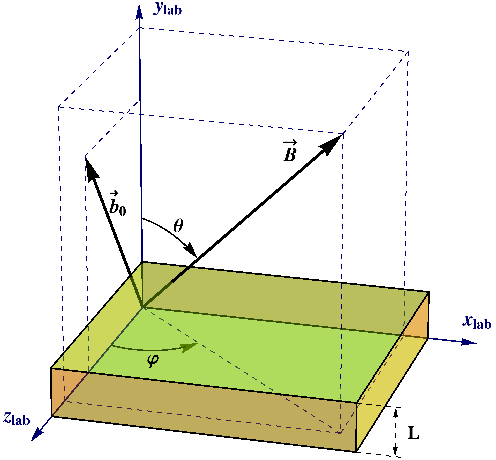

The Fermi arc states are localized on the surfaces of the semimetal and are characterized by wave vectors and . Since the velocities of these modes are parallel to the axis, only the component of the quasiclassical equation of motion in the magnetic field is nontrivial; i.e.,
| (739) | |||||
| (740) |
Therefore, the corresponding quasiparticles slide along the bottom (top) Fermi arc from the right-handed (left-handed) node at () to the left-handed (right-handed) node at (), where is the component of the chiral shift parallel to the surface of the semimetal. The surface parts of the quasiparticle orbits are connected with each other via the gapless bulk modes of fixed chirality. The corresponding closed orbits are schematically shown in Fig. 47, where we use a mixed coordinate–wave vector representation combining the out-of-plane axis with the in-plane and axes.
The semiclassical quantization condition for the closed orbits involving the Fermi arc modes reads [612]
| (741) |
where is an integer and is an unknown phase shift that can be determined only via the rigorous quantum analysis. The total time includes the time of quasiparticle propagation through the bulk , where the presence of is related to the fact that the movement through the bulk occurs only along the magnetic field, and the time it takes for the surface Fermi arcs to evolve from one chirality node to the other. The latter can be estimated from Eqs. (739) and (740), i.e., , where is the arc length in the reciprocal space. The latter is determined by the component of the (full) chiral shift parallel to the surface of the semimetal [612, 613]. Therefore, Eq. (741) implies that
| (742) |
If the Fermi energy is fixed and the magnetic field is varied, the density of states, associated with the corresponding close quasiclassical orbits, will be oscillating. The peaks of such oscillations occur when the Fermi energy crosses the energy levels in Eq. (742). Taking into account that , we derive the following discrete values of the magnetic field that correspond to the maxima of the density of state oscillations:
| (743) |
By noting that the expression on the right-hand side should remain positive definite, we conclude that the smallest possible value of is given by , where denotes the integer part. This corresponds to the saturation value of the magnetic field , above which no more oscillations will be observed.
In order to quantify the effects of interaction in the Weyl semimetal in a magnetic field, we will study how the density of states, involving the Fermi arc modes, oscillates as a function of the inverse magnetic field. In general, as the above analysis shows, the period of oscillations is given by
| (744) |
The interaction effects on the chiral shift were analyzed in Section 6.1.3 and can be summarized as follows. The full chiral shift takes the following form: , where is the chiral shift in absence of the magnetic field, is the magnitude of the correction to the chiral shift, and is the unit vector pointing in the direction of the field. Therefore, in the laboratory frame of reference, in which the component of the bare chiral shift vanishes, , the explicit expressions for the components of the full chiral shift in a Weyl semimetal in a magnetic field read
| (745) | |||||
| (746) | |||||
| (747) |
Since the length of the Fermi arcs is determined by the component of the chiral shift parallel to the surface, we include the effects of interaction in Eq. (744) by replacing the bare arc length with its interaction modified expression; i.e., . Then, by making use of Eqs. (745) and (747), we obtain our final result for the period of oscillations in the interacting case with an arbitrary oriented magnetic field
| (748) |
Since the Fermi arc length depends on the magnetic field, strictly speaking, the period will be drifting with the varying magnetic field. The numerical results for the period as a function of angle () are shown in the left (right) panels of Fig. 48 for several fixed values of angle (). [Note that we display only the results for because .] The thick (thin) lines represent the results with (without) taking interaction into account. To obtain these results we fixed the model parameters as follows: , , , , . In order to extract the qualitative effects in the cleanest form, let use a moderately strong coupling, . While such a set of model parameters is representative, it does not correspond to any specific material.


As seen from the numerical results in Fig. 48, the most important qualitative effect is the dependence of the oscillation period, which appears only in the case with interaction. The emergence of such a dependence is easy to understand from the physics viewpoint. Indeed, in the noninteracting theory, the chiral shift, as well as the length of the Fermi arcs associated with it, are independent of the magnetic field. The situation drastically changes in the interacting theory when a correction to the chiral shift parallel to is generated. As follows from Eq. (748), such a correction introduces a nontrivial dependence of the Fermi arc length on as soon as the component of the magnetic field parallel to the surface is nonzero (i.e., ). At , the period of quantum oscillations does not depend on because in this case the magnetic field is perpendicular to the surface of a semimetal and, therefore, . Also, as one can see on the left panel of Fig. 48 and in Eq. (748), the period of quantum oscillations vanishes at . In this case the component of the magnetic field perpendicular to the surface is absent and, therefore, the quasiclassical motion along the Fermi arcs is forbidden. The maximum value of the peak of the period of the oscillations as a function of takes place at
| (749) |
Measuring this angle in experiment would make it possible to determine the value of the ratio and, thus, quantify the interaction effects in Weyl semimetals. However, a complete fit of the angular dependence in Eq. (748) to the period obtained in experiment will allow us to extract not only , but also the value of if the chemical potential and the Fermi velocity are known.
7 Relativistic field theories in a magnetic background as noncommutative field theories
In this section, we will consider relativistic field theories in a magnetic background and their connection with the dynamics in noncommutative field theories (NCFT). (For reviews on NCFT, see Refs. [614, 615].) Our discussion is based on Refs. [616, 617].
Besides being interesting in themselves, noncommutative theories mimic certain dynamics in quantum mechanical models [618, 619], nonrelativistic field systems [620, 621], nonrelativistic magnetohydrodynamical field theory [622], and string theories [623, 624]. In particular, NCFT are intimately related to the dynamics in quantum mechanical and nonrelativistic field systems in a strong magnetic field [618, 619, 620, 621, 622] and, in the case of open strings attached to -branes, to the dynamics in string theories in magnetic backgrounds [624, 625].
In this section, we show that there is a deep connection between the dynamics in relativistic field theories in a strong magnetic field and that in NCFT. Our main conclusion is that although field theories in the regime with the lowest Landau level (LLL) dominance indeed determine a class of NCFT, these NCFT are different from the conventional ones. In particular, the UV/IR mixing, taking place in the conventional NCFT [626], is absent in this case. The reason of that is an inner structure (i.e., dynamical form-factors) of neutral composites in these theories.
In order to be concrete, two different types of the models (theories) are considered. In Section 7.1, the Nambu-Jona-Lasinio type models in a magnetic field are discussed, and in Section 7.2, the relativistic gauge field theories, QED and QCD, are considered. In Section 7.3, we summarize the main results and further elaborate on the connection between field theories in a magnetic field and NCFT. In Appendix F, some useful formulas and relations are derived.
7.1 The NJL model in a magnetic field as a NCFT
In this section, we will consider the -dimensional Nambu-Jona-Lasinio (NJL) models in a strong magnetic field for arbitrary spatial dimension . In the regime with the LLL dominance, we derive the effective action of the corresponding NCFT in the models with a large number of fermion colors and analyze their dynamics. It will be shown that these NCFT are consistent and quite sophisticated. An especially interesting case is that for a magnetic field configuration with the maximal number of independent nonzero tensor components [627, 74]. It will be shown that these NCFT are finite for even and their dynamics are quasi--dimensional for odd [for even , the NCFT describe a confinement dynamics of charged particles].
As will be shown, it is the LLL dominance that provides the exponentially damping (form-)factors which are responsible for finiteness of these NCFT for even and their quasi--dimensionality for odd . Thus, besides being low-energy theories of the NJL models in a strong magnetic field, the NCFT based on the LLL dynamics are self-contained and self-consistent.
Our approach uses two different sets of composite fields for the description of the dynamics. The first set uses the conventional composite fields and . In this case, besides the usual Moyal factor [614, 615], additional exponentially damping factors occur in the interaction vertices of the fields and . These factors reflect an inner structure of composites and play an important role in providing consistency of these NCFT. In particular, because of them, the UV/IR mixing is absent in these theories. In the second approach, one considers other, “smeared" fields and , connected with and through a nonlocal transformation. Then, while the additional factors are removed in the vertices of the smeared fields, they appear in their propagators, again resulting in the UV/IR mixing removal. By using the Weyl symbols [614, 615] of the smeared fields, we derive the effective action for the composites in the noncommutative coordinate space.
this section is organized as follows. In Section 7.1.1, in order to understand the nature of the modified NCFT in a clear and simple way, we discuss the quantum mechanical model in a magnetic field introduced in Ref. [619]. We show that besides the solution of Ref. [619], which mimics a conventional NCFT, there is another solution, with an interaction vertex containing exponentially damping factors. The existence of these two solutions reflects the possibility of two different treatments of the case with the particle mass in this model. In Section 7.1.2, the effective action of the NCFT connected with the -dimensional NJL model in a strong magnetic field is derived. In Section 7.1.3, the dynamics of this model is discussed. In Section 7.1.4, we generalize the analysis to a general case of dimensions with .
7.1.1 Nonrelativistic model
In order to understand better the nature of the modified NCFT, in this section we analyze a simple quantum mechanical two-dimensional system: a pair of unit charges of opposite sign (i.e., a dipole) in a constant magnetic field and with a harmonic potential interaction between them. This model was considered in Ref. [619]. It was argued there that for a strong magnetic field this simple system reproduces the dynamics of open strings attached to D-branes in antisymmetric tensor backgrounds.
We will show that important features of the modified NCFT occur already in this simple quantum mechanical model. Its Lagrangian reads
| (750) |
It is convenient to use the center of mass and relative coordinates, and , respectively. In these coordinates, Lagrangian (750) takes the form
| (751) |
The LLL dominance occurs when either or . Taking , the authors of [619] drop the kinetic terms in Lagrangian (751) that results in a theory of the Chern–Simons type with only first order time derivatives. Then, they introduce an additional potential describing an interaction of the first charge with an “impurity" centered at the origin and show that the matrix element of between dipole states contains the usual Moyal phase that is a signature of NCFT.
Notice that this result is obtained when the limit is taken directly in the Lagrangian. Let us now show that when one first solves this problem for a nonzero and then takes the limit in the solution, additional exponential factors occur in the matrix element of .
The Hamiltonian in model (750) is given by
| (752) |
where and are operators of the center of mass and relative momenta. Since the Hamiltonian is independent of the center of mass coordinates, the wave function can be represented in the form . Then, for we get the equation
| (753) |
Changing the variables to
| (754) | |||||
| (755) |
we arrive at the following equation:
| (756) |
Clearly, the first term here is the kinetic energy of the center of mass. Note that as , it coincides with the eigenvalue of the Hamiltonian in Ref. [619] obtained from Lagrangian (750) with . All other terms that are present in Hamiltonian (756) [and reflecting the inner structure of composite states] are absent in the Hamiltonian of Ref. [619]. In that case, the only information about the inner structure of composites that is retained is given by the relations
| (757) |
which express the relative coordinates in terms of the center of mass momentum.
Equation (756) describes a harmonic oscillator, and it can be solved exactly. Its spectrum contains an infinite number of composites (neutral bound states) with the energy eigenvalues
| (758) |
where , and and are nonnegative integers. Note that in the limit the Lagrangian (750) reduces to the Lagrangian of two noninteracting charged particles in a constant magnetic field (the Landau problem) and Eq. (758) correctly reproduces the Landau spectrum.
Thus, the model (750) describes an infinite number of neutral composites. The vector is their center of mass momentum and the last term in (758) reflects their nontrivial inner structure. Now, in the limit , only the LLL states with survive (all higher excitations decouple). The normalized LLL wave function with the center of mass momentum is given by
| (759) |
The Gaussian exponential factors here reflect the inner structures of the composites. It is important that in the limit , this wave function does not coincide with the wave function of Ref. [619] corresponding to the model with the Lagrangian (750) at : there are no Gaussian exponential factors in that case. In other words, while in the model, there are quantum fluctuations described by the Gaussian exponents, these fluctuations are completely suppressed in the model with .
Thus, we conclude that the quantum dynamics in the limit in the massive model does not coincide with that in the massless one. Recall that the same situation takes place in non-Abelian gauge theories: the limit in a massive non-Abelian model does not yield the dynamics of the massless one [628, 629, 630]. The origin of this phenomenon is the same in both cases. Because of constraints in the massless models, the number of physical degrees of freedom there is less than the number of degrees of freedom in the massive ones. In the present quantum mechanical model, these constraints are described by equation (757).
Of course, there is nothing wrong with the model (750) at . It is mathematically consistent. However, its dynamics is very different from that of a physical dipole in a strong magnetic field [by a physical dipole, we understand a dipole composed of two massive charged particle, including the case of an infinitesimally small mass ]. We also would like to point out that the present treatment of the dynamics in a strong magnetic field is equivalent to the formalism of the projection onto the LLL developed in Refs. [631, 632, 633].
If following Ref. [619] we introduce an additional potential describing an interaction of the first charge with an impurity, the matrix element will describe the scattering of composites on the impurity in the Born approximation. In order to evaluate , it is convenient to introduce the Fourier transform
| (760) |
so that
| (761) |
By making use of the completeness of eigenstates, i.e., , as well as Eq. (759), one can easily calculate the matrix element . In the limit , it is
| (762) |
with the cross product . One can see that, in addition to the standard Moyal factor , this vertex contains also the exponentially damping term . As is easy to check, this term originates from the Gaussian factors in the wave function (759). It would be absent if we, as in Ref. [619], used the Lagrangian with in Eq. (750).
The general character of this phenomenon suggests that additional exponential terms in interaction vertices should also occur in field theories in a strong magnetic field. This expectation will be confirmed in the next subsection, where it will be also shown that these theories determine a class of modified NCFT.
7.1.2 The effective action
In this section, we will consider the dynamics in the -dimensional NJL model in a strong magnetic field. Our aim is to show that this dynamics determines a consistent NCFT. As it will be shown in Section 7.1.4, a similar situation takes place in an arbitrary dimension with the space dimension .
Let us consider the same NJL model with the chiral symmetry as in Section 2.6. The Lagrangian density reads
| (763) |
cf. Eq. (120). Once again, we assume that the fermion fields carry an additional “color" index . The covariant derivative is , where the external vector potential describes a constant magnetic field pointing in the direction. We will use interchangeably the Landau gauge (3) and the symmetric gauge (157).
We will consider the dynamics of neutral bound states (“dipoles") in this model in the limit of large . In this limit, as we saw in Section 2.6, the model becomes essentially soluble, and its nonperturbative ground state is determined by the magnetic catalysis phenomenon.
At large , the relevant neutral degrees of freedom are connected with the composite fields and . The formal definition of the effective action for these fields was given in Eqs. (122) and (123) in Section 2.6. There we also derived an explicit form of the effective potential and the gap equation, see Eqs. (124) and (125), respectively. The latter, in particular, determines the dynamical mass of fermions, , which is nonzero for any positive .
Let us recall that the dynamics is dominated by the LLL in the weak coupling regime, with the dimensionless coupling constant . The expression for the fermion mass is given by Eq. (130), or equivalently
| (764) |
where is an ultraviolet cutoff connected with longitudinal momenta . We assume that . As will become clear below, there are no divergences connected with transverse momenta in the regime with the LLL dominance, and therefore the “longitudinal" cutoff removes all divergences in this model. Notice that Eq. (764) implies the following hierarchy of scales: . It will be shown in Section 7.1.3 that a meaningful continuum limit , with and a finite , exists in this model.
It is straightforward to calculate the interaction vertices for the quantum and fields that follow from the effective action, defined by Eqs. (122) and (123). For example, the 3-point vertex is given by
| (765) |
The fermion propagator is given as a product of the Schwinger phase factor, , and a translationally invariant part , see Eq. (923) in Appendix A.1. In the LLL approximation, the Fourier transform of the latter reads
| (766) |
[for convenience, the Kronecker -symbol with color indices is omitted in the propagator].
The explicit form of the Schwinger phase is given by
| (767) |
in the symmetric gauge (157), and by
| (768) |
in the Landau gauge (3). The Schwinger phase factor breaks the translation invariance even in the case of a constant magnetic field, although in this case there is a group of magnetic translations whose generators, unlike usual momenta, do not commute (for a more detailed discussion, see Section 2.8). One can easily check that the total phase along the closed fermion loop in (765) is independent of a gauge, i.e., the corresponding result is gauge invariant.
We will show that, in the regime with the LLL dominance, the effective action for the and fields, Eqs. (122) and (123), leads to a NCFT with noncommutative space transverse coordinates :
| (769) |
It is the Schwinger phase that is responsible for this noncommutativity. Indeed, the commutator is of course antisymmetric, and the only place where an antisymmetric tensor occurs in 3-point vertex (765) is the Schwinger phase (as will be shown below, a similar situation takes place also for higher vertices).
We begin our analysis with the observation that the LLL fermion propagator in coordinate space factorizes into two parts, the part depending on the transverse coordinates and that depending on the longitudinal coordinates :
| (770) |
Indeed, taking into account expressions (766) and (767), we get in the symmetric gauge:
| (771) |
and
| (772) |
[henceforth, for concreteness, we will use the symmetric gauge]. The longitudinal part is nothing else but a fermion propagator in 1+1 dimensions. In particular, the matrix is the projector on the fermion (antifermion) states with the spin polarized along (opposite to) the magnetic field, and therefore it projects on two states of the four ones, as should be in 1+1 dimensions. As to the operator , it is easy to check that it satisfies the relation
| (773) |
and therefore is a projection operator. Since is a LLL propagator, it is clear that is a projection operator on the LLL states.
The factorization of the LLL propagator leads to a simple structure of interaction vertices for and fields. For example, as it is clear from expression (765) for the 3-point vertex, a substitution of the Fourier transforms for the fields makes the integration over the longitudinal and transverse coordinates completely independent. And since is a -dimensional propagator, the integration over coordinates yields a fermion loop in the -dimensional Minkowski space. It is obvious that the same is true also for higher order interaction vertices arising from action (122). Therefore, the dependence of interaction vertices on longitudinal momenta is standard and, for clarity of the presentation, we will first consider the case with all external longitudinal momenta entering the fermion loop to be zero. This of course corresponds to the choice of and fields independent of longitudinal coordinates . The general case, with the fields depending on both transverse and longitudinal coordinates, will be considered in the end of this section.
Now, substituting the Fourier transforms of the fields and into Eq. (765) and using Eqs. (770), (771), and (772), we find the following expression for the 3-point interaction vertex in the momentum space:
| (774) | |||||
where , (here, for convenience, we omitted the subscript for the transverse coordinates). Notice that because of the exponentially damping factors, there are no ultraviolet divergences in this expression.
According to [614, 615], an -point vertex in a noncommutative theory in momentum space has the following structure:
| (775) |
where here denotes a generic field and the exponent is the Moyal exponent factor. Comparing expressions (774) and (775), we see that apart from the factor , the vertex coincides with the standard 3-point interaction vertex in a noncommutative theory with the commutator .
In order to take properly into account this additional factor in the vertex, it will be convenient to introduce new, “smeared” fields:
| (776) | |||||
| (777) |
where is the transverse Laplacian. Then, in terms of these fields, the vertex can be rewritten in the standard form with the Moyal exponent factor:
| (778) |
One can similarly analyze the 4-point interaction vertex . We get
| (779) |
The occurrence of the smeared fields in the vertices reflects an inner structure (dynamical form-factors) of and composites on the lowest Landau level, which is similar to that of a dipole in the quantum mechanical problem considered in Section 7.1.1.
As is well known, the cross product in the momentum space corresponds to a star product in the coordinate space [614, 615]:
| (780) |
where here represents the smeared fields and . By using the star product, one can rewrite the vertices and in the following simple form in the coordinate space:
| (781) | |||||
| (782) |
As to expressing the vertices in NCFT in the space with noncommutative coordinates , one should use the Weyl symbol of a field there [614, 615]:
| (783) | |||||
| (784) |
The most important property of the Weyl symbol is that the product of the Weyl symbols of two functions is equal to the Weyl symbol of their star product:
| (785) |
In our case, the Weyl symbol represents and . Note that the relation between the Weyl symbols of smeared and non-smeared fields is
| (786) |
where the operator in the noncommutative space acts as
| (787) |
[the latter relation follows from the definition of the derivative in NCFT, [614, 615] ].
In terms of , the 3- and 4-point vertices take the following form in NCFT:
| (788) | |||||
| (789) |
where the operation is defined as in Refs. [614, 615]. As is shown in Appendix F.1, all interaction vertices () arising from action (122) have a similar structure.
There exists another, more convenient for practical calculations, representation of interaction vertices in which the vertices are expressed through the initial, non-smeared, fields and . The point is that, due to the presence of the -function , the exponent factors in an -point vertex can be rewritten as , where is a new cross product. It is defined as
| (790) |
with the matrix being
| (791) |
We will call an (magnetic)-cross product. Notice that like the matrix , defining the cross product, the new matrix , defining the -cross product, is anti-hermitian. [Note that in the mathematical literature, the -cross product is called the Voros product [634, 635].]
By using the -cross product, we get the following simple structure for an -point vertex in the momentum space:
| (792) |
[compare with expression (775)]. Here the field represents initial fields and .
In the coordinate space, the -cross product becomes an -star product:
| (793) |
[compare with equation (780)]. By using the -star product, one can express -point vertices through the initial and fields in the coordinate space. For example, the vertices and become:
| (794) | |||||
| (795) |
In fact, by using the -star product, the whole effective action (122) can be written in a compact and explicit form for the case of fields independent of longitudinal coordinates . First, note that for constant fields, the -star product in vertices (795) is reduced to the usual product and the vertices come from the effective potential in that case. Then, this implies that, up to the measure , the whole effective action for fields depending on transverse coordinates coincides with the effective potential in which the usual product is replaced by the -star product in the part coming from the term in (122). As to the last term there, it should stay as it is. This is because unlike the star product, the -star product and the usual one lead to different quadratic terms in the action. Now, by using expression for the fermion propagator, we easily find the effective potential:
| (796) |
[Note that this agrees with the effective potential in Eq. (124) in the limit of weak coupling when .] Then, the effective action reads:
| (797) |
This expression is very convenient for calculating the -point vertices [636]. In Appendix F.2, it is shown that the -star product also naturally appears in the formalism of the projected density operators developed in Ref. [636] for the description of the quantum Hall effect.
While the -star product is useful for practical calculations, its connection with the multiplication operation in a noncommutative coordinate space is not direct. This is in contrast with the star product for which relation (785) takes place. Therefore, it will be useful to rewrite action (797) through the star product. It can be done by using the smeared fields and . The result is
| (798) |
where we used the fact that the star product and the usual one lead to the same quadratic terms in the action. Notice that the fields and are connected with the smeared fields through the nonlocal relation (777). This relation implies that exponentially damping form-factors are built in the propagators of the smeared fields. As a result, their propagators decrease rapidly, as , with . As will be shown in the next subsection, this property is in particular responsible for removing the UV/IR mixing in the model.
By using relation (785), it is straightforward to rewrite the action in the NCFT through Weyl symbols:
| (799) |
The Weyl symbols and are connected with the Weyl symbols and through relation (786).
Let us now generalize expressions (797), (798), and (799) to the case when fields and depend on both transverse and longitudinal coordinates. First, as it follows from the expansion of the -term in action (122) in a series in and , the general -point vertex is given by
| (800) | |||||
[notice that here the longitudinal part of the fermion propagator does not contain color indices]. As was shown above and in Appendix F.1, the transverse part of vertex (800) can be expressed through the -star product. Therefore, the -point vertex is
| (801) | |||||
This relation implies that the full effective action can be written through the -star product as:
| (802) |
where the projector is
| (803) |
(compare with action (797)). Here the trace , related to the longitudinal subspace, is taken in the functional sense.
As to the form of the effective action written through the star product and its form in the noncommutative coordinate space, they are:
| (804) |
and
| (805) |
This concludes the derivation of the action of the noncommutative field theory corresponding to the NJL model in a strong magnetic field. In the next subsection, we will consider the dynamics in this model in more detail.
7.1.3 The low-energy dynamics
In the regime with the LLL dominance, the dynamics of neutral composites is described by quite sophisticated NCFT (805). In this section, we will show that in this model (i) there exists a well defined commutative limit when ; (ii) the universality class of the low-energy dynamics, with , is intimately connected with the dynamics in the -dimensional Gross-Neveu (GN) model [223]; and (iii) there is no UV/IR mixing.
The key point in the derivation of action (805) was the fact that the LLL fermion propagator factorizes into two parts [see Eq. (770)] and that its transverse part is a projection operator on the LLL states. It is quite remarkable that it exactly coincides with the projection operator on the LLL states in nonrelativistic dynamics introduced for the description of the quantum Hall effect in Refs. [631, 637]. This feature is, of course, intimately connected with the fact that the wave functions of the LLL states are independent of the fermion mass [see Eq. (759) for ]. Therefore, the transverse dynamics in this problem is universal and peculiarities of the relativistic dynamics reflect themselves only in the -dimensional longitudinal space.
In order to study the low-energy dynamics with , it will be instructive to consider, as in Ref. [83], the following continuum limit: , with and being fixed. Let us consider -point vertex (800) in this limit. Since the projection operator is
| (806) |
(see Eq. (771)), the point with coordinates , , is both a saddle and stationary point in the multiple integral (800) in the limit . Therefore, in order to get the leading term of the asymptotic expansion of that integral, one can put in the arguments of all the fields there. Then, by using relation (773) and the equality , we easily integrate over transverse coordinates in (800) and obtain the following asymptotic expression:
| (807) | |||||
This equation implies that as , the leading asymptotic term in the action is
| (808) |
This action corresponds to a commutative field theory, as should be in the limit [indeed, the commutator goes to zero as ]. Also, since there is no hopping term for the transverse coordinates in this action, they just play the role of a label of the fields.
Let us now compare this action with the action of the -dimensional GN model [223]:
| (809) |
where is a dimensionless coupling constant. One can see that, up to the factor , these two actions coincide if the constant in (808) is identified with . In particular, with this identification, expression (764) for the dynamical mass coincides with the expression for in the GN model, . Also, using Eq. (764), one can express the coupling constant in the effective potential (796) through the dynamical mass and cutoff . Then, up to terms, we get the expression independent of the cutoff:
| (810) |
This renormalized form of the potential coincides with the GN potential.
As to the factor , its meaning is very simple. Since density of the LLL states is equal to , this factor yields the number of the Landau states on the transverse plane. In other words, as , the model is reduced to a continuum set of independent -dimensional GN models, labeled by the coordinates in the plane perpendicular to the magnetic field. The conjecture about such a structure of the NJL model in the limit was made in Ref. [83] and was based on a study of the effective potential and the kinetic (two derivative) term in the model. The present approach allows us to derive the whole action and thus to prove the conjecture.
The existence of the physically meaningful limit is quite noticeable. It confirms that the model with the LLL dominance is self-consistent. In order to understand its dynamics better, it is instructive to look at the dispersion relations for and excitations with momenta (see Section 2.6):
| (811) | |||||
| (812) |
We find from these relations that the transverse velocity of both and goes rapidly [as )] to zero as . In other words, there is no hopping between different transverse points in this limit. For a strong but finite magnetic field, the transverse velocity is, although nonzero, very small. In this case, the and composites have a cigar-like shape: while their transverse size is of the order of the magnetic length , the longitudinal size is of order , and .
The important point is that besides being a low-energy theory of the initial NJL model in a magnetic field, this truncated [based on the LLL dynamics] model is self-contained. In particular, in this model one can consider arbitrary large values for transverse momenta , although in this case its dynamics is very different from that of the initial NJL model. In fact, by using the expression for the pion propagator (818) written below, it is not difficult to check that for the dispersion relation for excitations takes the following form:
| (813) |
In this regime, the transverse velocity is extremely small, , and a excitation is a loose bound state moving along the direction. Its mass is close to the threshold.
Thus, we conclude that the NJL model in a strong magnetic field yields an example of a consistent NCFT with quite nontrivial dynamics. The point that exponentially damping factors occur either in vertices (for the fields and ) or in propagators (for the smeared fields) plays a crucial role in its consistency. Let us now show that these factors are in particular responsible for removing a UV/IR mixing, the phenomenon that plagues conventional nonsupersymmetric NCFT [626].
The simplest example of the UV/IR mixing is given by a one-loop contribution in a propagator in the noncommutative model with the action
| (814) |
There are planar and nonplanar one-loop contributions in the propagator of in this model [626]:
| (815) |
The nonplanar contribution is specific for a noncommutative theory and is responsible for the UV/IR mixing. Indeed, the nonplanar contribution is equal to
| (816) |
where
| (817) |
with being cutoff. It is clear that if the external momentum , the nonplanar contribution (816) diverges quadratically. On the other hand, for a nonzero , it is finite due to the Moyal phase factor in the second term in expression (815) (which oscillates rapidly at large ). Thus, although the Moyal factor regularizes the UV divergence, it leads to an IR divergence of the integral, i.e., to the UV/IR mixing.
Let us now show how the exponentially damping factors in vertices (for the fields and ) or in propagators (for the smeared fields and ) remove the UV/IR mixing. We will first consider the description using the fields and . As an example, we will consider the one-loop correction in the propagator generated by the four-point interaction vertex . First, from action (122), we get this propagator in tree approximation. In Euclidean space it is
| (818) |
Then, by using this and Eq. (801) for the vertex , we find the following one-loop nonplanar contribution to the propagator:
| (819) |
where
Here the integral over transverse momenta is
| (820) |
It is clear that due to the presence of the factor and because is finite as , this integral is convergent for all values of , including , and therefore there is no UV/IR mixing in this case. On the other hand, if the factor were absent in integrand (820), we would get the integral
| (821) |
which diverges quadratically at , i.e., the UV/IR mixing would occur.
Let us now turn to the description using the smeared fields. The relation (777) between the fields and implies that their propagators are related as
| (822) |
Since is an entire function, the absence of the UV/IR mixing in the propagator implies that there is no UV/IR mixing also in the propagator . This conclusion can be checked directly, by adapting the calculations of the one-loop correction in the propagator to the propagator. In this case, it is the form-factor , built in the propagator , that is responsible for the absence of the UV/IR mixing.
This concludes the analysis in dimensions. In the next subsection, we will generalize this analysis to arbitrary dimensions with .
7.1.4 Beyond 3+1 dimensions
In this section, we will generalize our analysis to arbitrary dimensions with . We begin by considering the NJL model in a magnetic field in dimensions, choosing its Lagrangian density similar to that in 3 + 1 dimensions:
| (823) |
Here a reducible four-dimensional representation of the Dirac matrices is used (for details, see Section 2). In a weak coupling regime, the dynamical mass in this model is (see Section 2.4.1)
| (824) |
The LLL propagator is obtained from the -dimensional propagator by just omitting the and variables there:
| (825) |
where, instead (772), the expression for is:
| (826) |
The analysis now proceeds as in the dimensional case. The present model corresponds to a noncommutative field theory describing neutral composites and . Its action written through the star product is
| (827) |
where and are smeared fields (compare with Eq. (804)). The action can be also written directly in the noncommutative coordinate space:
| (828) |
(compare with Eq. (805)).
In the previous Sections, it was shown that in the regime with the LLL dominance, the divergences in (3 + 1)-dimensional model are generated only by the -dimensional longitudinal dynamics. For the (2 + 1)-dimensional model in this regime, a stronger statement takes place: the model is finite. It can be shown by repeating the analysis used in 3 + 1 dimensions. In particular, in the continuum limit , the effective potential in this model is finite without any renormalizations:
| (829) |
Using Eq. (824), one can express the coupling constant in the potential through and . Then, the potential takes an especially simple form:
| (830) |
For momenta , the dispersion relation for excitations is (see Section 2.4.2):
| (831) |
Therefore, as in dimensions, the velocity is strongly suppressed: in the present case it is of order . As to the excitation, its "mass", defined as the energy at zero momentum, is very large: (see Section 2.4.2). Therefore, the -mode decouples from the dynamics with .
As in the case of dimensions, this truncated [based on the LLL dynamics] model is self-contained and one can consider arbitrary large values for momenta there. It is easy to check that for the dispersion relation for excitations takes the form
| (832) |
In this regime, the velocity becomes extremely small, , and a excitation is a loosely bound state. Its mass is close to the threshold.
As was shown in Section 7.1.3, in the limit the -dimensional model is reduced to a continuum set of independent (1+1)–dimensional Gross–Neveu models labeled by the coordinates in the plane perpendicular to the magnetic field. Similarly to that, in the case of 2 + 1 dimensions, in the limit the model is reduced to a set of (0+1)- dimensional (i.e., quantum mechanical) models labeled by two spatial coordinates.
A new feature of the -dimensional model is a confinement dynamics for charged particles: they do not propagate in a magnetic background. On the other hand, since neutral composites are free to propagate in a magnetic field, one can define asymptotic states and -matrix for them. The -matrix should be unitary in the subspace of neutral composites.
Let us now consider the case of higher dimensions with . First of all, recall that for an even , by using spatial rotations, the noncommutativity tensor in a noncommutative theory with can be reduced to the following canonical skew-diagonal form with skew-eigenvalues [614, 615]:
| (833) |
If is odd, then the number of canonical skew-eigenvalues of is equal to , where is the integer part of , and the canonical form of is similar to (833) except that there are additional one zero column and one zero row.
On the other hand, a constant magnetic field in dimensions is also characterized by independent parameters, and the strength tensor can be also reduced to the canonical skew-diagonal form [627, 74]:
| (834) |
The corresponding nonzero components of the vector potential are equal to
| (835) |
Thus, we see that there is one-to-one mapping between the skew-eigenvalues of the noncommutativity tensor and the independent parameters of the spatial part of the electromagnetic strength tensor in a space of any dimension .
Chiral symmetry breaking in the NJL model in a strong magnetic field in dimensions with was studied in Ref. [74]. By using results of that paper, it is not difficult to extend our analysis in and dimensions to the case of . The crucial point in the analysis is the structure of the Fourier transform of the translationally invariant part of the LLL propagator. If all are nonzero, one can show that it is
| (836) |
where if is even and if is odd. If some , then, for each , the longitudinal part gets two additional components, and , and the corresponding terms are absent in the transverse part of expression (836). Thus, like in and dimensions, the LLL propagator factorizes into the transverse and longitudinal parts. The projection operator on the LLL is now equal to the direct product of the projection operators (771) in the -planes with nonzero [here the subscript is the number of nonzero independent components of ].
Because of that, it is clear that the NJL model in a strong magnetic field in a space of arbitrary dimensions corresponds to a noncommutative field theory with parameters expressed through the magnetic part of the strength tensor . Its action is [compare with expressions (805) and (828)]:
| (837) |
where is the number of nonzero independent components of and the projector equals the direct product of projectors (803) in the -planes with nonzero . In particular, for a magnetic field configuration with the maximal number of independent nonzero tensor components, the dynamics is quasi--dimensional for odd and finite for even . In the latter case the model describes a confinement dynamics of charged particles. Also, as all , the model is reduced either to a continuum set of -dimensional GN models labeled by spatial coordinates (odd ) or to a set of quantum mechanical models labeled by spatial coordinates (even ).
In the next section, we will describe the connection between gauge theories in a magnetic field and NCFT. It will be shown that in that case this connection is more sophisticated and interesting than that for the NJL model.
7.2 Gauge theories in a magnetic field as NCFT
In the previous section, the connection between the dynamics in the NJL model in a strong homogeneous magnetic field and that in NCFT has been studied. The main conclusion was that although relativistic field theories in the regime with the lowest Landau level (LLL) dominance indeed determine a class of NCFT, these NCFT are different from the conventional ones considered in the literature. In particular, the UV/IR mixing, taking place in the conventional NCFT [626], is absent in these theories. The reason of that is an inner structure (i.e., dynamical form factors) of electrically neutral composites in these theories. We emphasize that in order to establish the connection between dynamics in a homogeneous magnetic field and dynamics in NCFT, it is necessary to consider neutral fields. The point is that in homogeneous magnetic backgrounds, momentum is a good quantum number only for neutral states and therefore one can introduce asymptotic states and S-matrix only for them.
While studies of the origins of the noncommutativity in relativistic quantum field theories in a magnetic field are interesting in themselves, it is even more important that they lead to new physical results. In particular, as was shown in Section 7.1.2, the NCFT approach allows one to derive interaction vertices for neutral composites. These vertices automatically include [in the form of the cross (Moyal) product, see Section 7.1.2] all powers of transverse derivatives [i.e., the derivatives with respect to coordinates orthogonal to a magnetic field]. This result is quite noticeable because the dimension of the transverse subspace is two and it is very seldom that one can with a good accuracy calculate vertices for composites in quantum field models with spatial dimensions higher than one.
In the analysis in Section 7.1, it was shown that there exist two equivalent descriptions of the dynamics of the NJL model in a magnetic field as NCFT. In the first description, one uses the conventional composite operators and . In this case, besides the usual Moyal factor, the additional Gaussian-like (form-)factor occurs in -point interaction vertices of the fields and . Here is a momentum of the -th composite in a plane orthogonal to the magnetic field. This form factor reflects an inner structure of composites and play an important role in providing consistency of the NCFT. In particular, because of them, the UV/IR mixing is absent in these theories.
In the second description, one considers other, “smeared" fields and , connected with and through a nonlocal transformation. Then, while the additional factors are removed in the vertices for the smeared fields, they appear in their propagators, again resulting in the UV/IR mixing removal.
The Gaussian form of the exponentially damping form factors reflects the Landau wave functions of fermions on the LLL. The form factors are intimately connected with the holomorphic representation in the problem of quantum oscillator (for a review of the holomorphic representation, see Ref. [638]). Indeed, in the problem of a free fermion in a magnetic field, the dynamics in a plane orthogonal to the magnetic field is an oscillator-like one.33 3 In particular, the holomorphic representation is widely used for the description of the quantum Hall effect [631, 632]. And because weak short-range interactions between fermions in the NJL model in a magnetic field do not change this feature of the dynamics, the form factors in that model have the Gaussian form.
But what happens in the case of more sophisticated dynamics, such as those with long-range interactions in gauge models? To find the answer to this question is the primary goal of this section.
To answer this question, we will extend the analysis of Section 7.1 to the more complicated cases of QED and QCD in a strong magnetic field. It will be shown that in these gauge models, the connection of the dynamics with NCFT is much more sophisticated than that in the NLJ model. It is not just that the damping form-factors are not Gaussian in these models but there does not exist an analogue of the smeared fields at all. As a result, their interaction vertices cannot be transformed into the form of vertices in conventional NCFT. On the other hand, it is quite remarkable that, by using the Weyl symbols of the fields (see Section 7.1), their vertices can nevertheless be represented in the space with noncommutative spatial coordinates. The dynamics they describe correspond to complicated nonlocal NCFT. We will call these theories type II nonlocal NCFT. The name type I nonlocal NCFT will be reserved for models similar to the NJL model in a magnetic field, for which smeared fields exist. In both these cases, the term “nonlocal" reflects the point that, besides the Moyal factor, additional form factors are present in the theories.
The crucial distinction between these two types of models is in the characters of their interactions. While the interaction in the NJL-like models is local (short-range), it is long-range in gauge theories. This point is reflected in a much richer structure of neutral composites in the latter. We believe that both these types of nonlocal NCFT can be relevant not only for relativistic field theories but also for nonrelativistic systems in a magnetic field. In particular, while type I NCFT can be relevant for the description of the quantum Hall effect in condensed matter systems with short-range interactions, type II NCFT can be relevant in studies of this effect in condensed matter systems with long-range interactions (such as carbon materials).
7.2.1 Chiral symmetry breaking in QED in a magnetic field
The central dynamical phenomenon in relativistic field theories in a magnetic field is the phenomenon of the magnetic catalysis. For QED, it was discussed in detail in Section 3.1. In this section, we will briefly describe those features of this phenomenon in QED, which are relevant for the present purposes.
The crucial point of the analysis in Section 3.1 was to recognize that there exists a special nonlocal (and non-covariant) gauge in which the improved rainbow (ladder) approximation is reliable in this problem, i.e., there is a consistent truncation of the system of the Schwinger–Dyson equations. We recall that in the improved rainbow (ladder) approximation the vertex is taken to be bare and the photon propagator is taken in the one-loop approximation. The full photon propagator in this gauge has the form [compare with (228)]
| (838) |
where is the polarization operator and the symbols and in and are related to the transverse and longitudinal space-time components, respectively (we consider a constant magnetic field directed in the direction). Because of the spin polarization for the positively (negatively) charged LLL fermion states along (opposite) to the magnetic field, the transverse degrees of freedom decouple from the LLL dynamics, and only the first term in photon propagator (838), proportional to , is relevant. Therefore, as the full photon propagator in this special gauge, one can take the Feynman-like noncovariant propagator
| (839) |
It is important that this propagator does not lead to infrared mass singularities in loop corrections in a vertex (see Section 3.1) that makes the improved rainbow approximation to be reliable in this gauge (because of mass singularities in covariant gauges, the loop corrections in the vertex are large there.).
As was pointed in Section 3.1, because the kinematic region is mostly responsible for generating the fermion mass, the polarization operator can be calculated in one-loop approximation. It is
| (840) |
where . Here is the number of fermion flavors and is the QED running coupling related to the magnetic scale .
In this approximation, photon propagator (839) becomes a propagator of a free massive boson with :
| (841) |
The corresponding approximation is reliable when the parameter is small, i.e., . The dynamically generated mass of fermions is
| (842) |
where , and is a numerical constant of order one. [This is the same as the expression in Eq. (241), but with the replacement .]
7.2.2 The effective action of QED in a magnetic field
In this section, we analyze the dynamics in the chiral symmetric QED in a strong magnetic field. We will consider both the weakly coupling regime, with , and (for large ) the strongly coupling regime with . In both these cases, one can use the results of the analysis in Section 3.1.
The chiral symmetry in this model is . The generation of a fermion mass breaks this symmetry down to and, as a result, neutral Nambu-Goldstone (NG) composites , , occur (we do not consider here the anomalous ). Our aim in this section is to derive the interaction vertices for in the regime with the LLL dominance and clarify whether their structure corresponds to a NCFT.
Integrating out the photon field , we obtain the following nonlocal effective action for fermions in QED in a magnetic field:
| (844) |
where, in the lowest order, the bare propagator corresponding to propagator (839) is
| (845) |
and the vector potential in the covariant derivative in (844) describes a constant magnetic field directed in the direction. The vector potential here is assumed to be in the symmetric gauge (157). Following the auxiliary field method developed for theories with nonlocal interaction in Refs. [639, 640], we add the term
| (846) |
in the action. Here is a bilocal auxiliary field with the indices and from the fundamental representation of . Then, we obtain the action
| (847) | |||||
[here, for clarity of the presentation, we omitted the indices]. Integrating over fermions, we find
| (848) | |||||
where and Ln are taken in the functional sense.
Following Ref. [640], we can expand as
| (849) | |||||
| (850) |
Here satisfies the equation
| (851) |
which is equivalent to the Schwinger–Dyson equation
| (852) |
where is the bare fermion propagator and is the full fermion propagator in the rainbow (ladder) approximation. As to Eq. (850), is a field operator describing a neutral composite and are solutions of the off-mass-shell Bethe–Salpeter equation in the ladder approximation,
| (853) |
The insertion of factor in this equation allows us to consider off-mass-shell states with an arbitrary mass . The on-mass-shell states correspond to .
Using Eqs. (849) and (852), the action (848) can be rewritten as
| (854) | |||||
Expanding now the action in powers of and ignoring its part that does not depend on , we obtain
| (855) | |||||
where
| (856) |
Because satisfies the Schwinger–Dyson equation (851), the term linear in is absent in (855).
As is clear from the discussion in Section 7.2.1, one should use the improved rainbow (ladder) approximation in the present problem. The Schwinger–Dyson equation for the fermion propagator in this approximation takes the form
| (857) |
where the photon propagator is given in Eq. (841). The off-mass-shell Bethe-Salpeter equation in the improved ladder approximation is given by
| (858) |
The comparison of Eqs. (857), (858) with Eqs. (852), (853) suggests that in the improved rainbow (ladder) approximation the effective action (855) should be replaced by the following one:
| (859) | |||||
where
| (860) |
and
| (861) |
(compare with Eq. (850)). Here are solutions of the off-mass-shell Bethe-Salpeter equation (858).
As in the case of the NJL model (see Section 7.1), the LLL fermion propagator in the improved rainbow approximation in QED factorizes into two parts: the part depending on the transverse coordinates and that depending on the longitudinal coordinates ,
| (862) |
Here the projection operator on the LLL states 7.1, which in the symmetric gauge is
| (863) |
The first exponential factor in is the Schwinger phase [42]. Its presence is dictated by the group of magnetic translations in this problem (for more details, see Section 7.3). As was shown in Section 7.1, it is the Schwinger phase that is responsible for producing the Moyal factor (a signature of NCFT) in interaction vertices.
As to the longitudinal part, in the improved rainbow approximation it has the form [119, 121, 128]
| (864) |
i.e., it has the form of a fermion propagator in 1+1 dimensions. The dynamical mass function is essentially constant for and rapidly decreases for [119, 121, 128]. Therefore, a simple and reliable approximation for is
| (865) |
where is the step function and is the fermion pole mass (842) or (843). [This conclusion was later confirmed in Refs. [125, 101].]
The operators in equation (861) describe all possible neutral fermion-antifermion composites. The description of their interaction vertices in QED in a magnetic field is quite a formidable problem. Henceforth, we limit ourselves to considering only the interaction vertices for the NG boson states and their operators . For a brief discussion concerning other states, see Section 7.3.44 4 As is well known, in some approximations, the Bethe-Salpeter equation is plagued by the appearance of spurious solutions. Because we restrict ourselves to calculating the vertices for the NG bosons, which are manifestly physical, no such problem occurs in this study.
In a magnetic field, the wave function of the states satisfying Bethe-Salpeter equation (858) has the following form [113]:
| (866) |
where , and, that is very important, the function is independent of the center of mass coordinate . This fact reflects the existence of the group of magnetic translations in the present problem. As in the case of the fermion propagator, the presence of the Schwinger factor in expression (866) is dictated by this symmetry (see Section 7.3). As to the structure of , it is
| (867) |
where are matrices in the fundamental representation of .
Now, transforming Bethe-Salpeter equation (858) into momentum space, we get
| (868) | |||||
where is the Moyal cross product. Then, introducing the variable and representing the wave function as
| (869) |
we integrate over in (868) and find the following equation for the function :
| (870) | |||||
Because the right hand side of equation (870) does not contain , we conclude that does not depend on , i.e., it is a function of and only. [It is not difficult to convince yourself that this fact is a direct consequence of the factorization of the LLL propagator.] Therefore, we can explicitly integrate over and get
| (871) |
Henceforth, we will consider the dynamics for the case of zero longitudinal momenta, , i.e., for , when the function in Eq. (861) is
| (872) |
with the Bethe-Salpeter wave function depending only on . For , the Fourier transform of the fields in coordinate space depends only on the coordinates . Because in this problem the noncommutative geometry is connected only with the transverse coordinates, this dependence is the most relevant for our purposes. The case with nonzero longitudinal momenta is quite cumbersome and is considered in the Appendix F.3.
We would like to emphasize that in the case of nonlocal interactions, such as those in QED, the bound state problem with nonzero is quite formidable. In fact, as will become clear below (see also Appendix F.3), it is the very special property of the factorization of the longitudinal and transverse dynamics in the LLL approximation that will allow us to succeed in the derivation of explicit expressions for interaction vertices for NG fields for nonzero .
When , one can check that, up to the factors and , the structure of equation (871) is similar to the Bethe-Salpeter equation for NG bosons with considered in Ref. [113]. By using the analysis performed in that work, we immediately find that
| (873) |
where is a scalar function. It satisfies the following equation in Euclidean space:
| (874) |
In the derivation of this equation, Eq. (841) was used.
Now, taking into account Eqs. (866), (869), and (873), and integrating explicitly over , we find that the Bethe-Salpeter wave function in coordinate space is
| (875) |
Then, inserting the bilocal field from Eq. (872) into action (859) and using the Bethe-Salpeter equation (858), we obtain the following explicit form for the effective action:
| (876) | |||||
From the effective action (876), one can obtain the -point vertices of NG bosons. In fact, using Eq. (875), the factorized form of the fermion propagator (862), and the fact that is a projection operator, we can integrate over all coordinates in the effective action (876), similarly as it was done in the case of the NJL model in Section 7.1.2. Then, we get the following expression for the effective action:
| (877) |
where the interaction vertices , , are
| (878) | |||||
and the quadratic part of the action is
| (879) | |||||
For the expressions of the vertices in the case of nonzero longitudinal momenta, see Appendix F.3.
In the next subsection, we will discuss the connection of the structure of vertices (878) with vertices in NCFT.
7.2.3 Type I and Type II Nonlocal NCFT
The derivation of the expressions for vertices (878) and quadratic part of the action (879) is one of the main results of this section (the generalization of these expressions for the case of nonzero longitudinal momenta are given in Eqs. (1122) and (1123) in Appendix F.3). Let us discuss the connection of the structure of these vertices with vertices in NCFT. According to [614, 615], an -point vertex in a noncommutative theory in momentum space has the following canonical form:
| (880) |
where here denotes a generic field and the exponent is the Moyal exponent factor. Here the antisymmetric matrix determines the commutator of spatial coordinates:
| (881) |
When can the vertex (878) be transformed into the conventional form (880)? In order to answer this question, it will be convenient to ignore for a moment the fact that in (878) is a solution of equation (874) and consider it as an arbitrary function of the momenta and . Then, comparing expressions (878) and (880), it is not difficult to figure out that if the function , defined as
| (882) |
has the factorized form
| (883) |
then there exists a map of the fields into new fields in terms of which vertices (878) take the conventional form (880). Indeed, let us introduce new fields
| (884) |
Then, after integrating over and taking trace over Dirac matrices, we get the conventional form for :
| (885) |
where and is some constant. The propagator of these fields is determined from the quadratic part (879) of the action:
| (886) |
Thus, in terms of the new fields , vertices (878) can be transformed into the canonical form. As will be shown in the next subsection, there exists a special dynamical regime in QED with a large number of fermion flavors and in which the constraint (883) can be fulfilled. In fact, this dynamical regime is essentially the same as that in the NJL model in a strong magnetic field (see Section 7.1). In this case, the function (882) is independent. Following Ref. [616], the fields with a built-in form factor will be called smeared fields.
In coordinate space, the interaction vertices (885) of the smeared fields take the form:
| (887) |
where the symbol is the conventional star product [614, 615] relating to the transverse coordinates. In the space with noncommutative transverse coordinates , , these vertices can be represented as
| (888) |
where is the Weyl symbol of the field , the operation is defined as in Refs. [614, 615], and
| (889) |
We will refer to theories with a factorized function as type I nonlocal NCFT.
In the case when the function in Eq. (882) is not factorized, one cannot represent interaction vertices (878) in the form of vertices of a conventional NCFT. This is the case for in the integral equation (874) with (see Section 7.2.5). However, even in this case, we still can represent vertex (878) as a nonlocal vertex in the noncommutative space. Indeed, we can rewrite (878) as
| (890) |
where the coincidence limit is taken after the action of a nonlocal operator on the fields . In momentum space, the operator is
| (891) |
By using the fact that the Weyl symbol of the derivative in noncommutative space is given by the operator acting as [614, 615]
| (892) |
we obtain the following form for the interaction vertices in the noncommutative space:
| (893) |
It is clear that NCFT with such vertices are much more complicated than type I nonlocal NCFT discussed above. We will call them type II nonlocal NCFT. As will be shown in Sections 7.2.5 and 7.2.6, QED and QCD in a strong magnetic field yield examples of such theories. For the case of nonzero longitudinal momentum , the counterparts of expressions (890) and (893) are derived in the Appendix F.3 (see Eqs. (1124) and (1126) there).
7.2.4 QED with large in a strong magnetic field and NCFT: dynamical regime with local interactions
Let us now consider the dynamical regime with such large that the expansion is reliable, and the coupling is so strong that in (841) is of order or larger. In this case, we have a NJL model with the current-current local interaction, in which the coupling constant and the ultraviolet cutoff connected with longitudinal momenta is (see Ref. [128]). The dynamical fermion mass is now given by expression (843) and the mass function is a constant, . In this regime, Eq. (874) takes the form
| (894) |
where the function is defined in Eq. (882). The subscript in reflects the consideration of the limit with local interactions here. Since the right-hand side of equation (894) does not depend on , the function is -independent, , i.e., this dynamics relates to the type I nonlocal NCFT considered in the previous section. Then, we immediately find from (894) that
| (895) |
where we used . Using now the on-mass-shell condition , for the NG bosons in equation (895), we arrive at the following gap equation for :
| (896) |
This gap equation yields expression (843) for the mass. It also implies that (895) can be rewritten in a very simple form:
| (897) |
The choice of the off-mass-shell operators in expansion (872) is not unique. They are determined by the choice of their propagator. If one chooses the conventional composite NG fields as , their propagator is
| (898) |
Up to a factor of , this propagator coincides with that in the NJL model in a magnetic field, see Section 7.1 and Ref. [616].55 5 In Ref. [616], the NJL model with fermion colors and the chiral group was considered. Therefore, when comparing with the results of Ref. [616], here one should take and replace the flavor matrices by . Since , there is an additional factor in the propagator of in the present model.
Interaction vertices (878) are nonzero only for even and they take now the form
| (900) |
where . These expressions for the vertices agree with those found in Section 7.1 (see footnote 5).
Apart from the exponentially damping factor , the form of these vertices coincide with that in NCFT with noncommutative space transverse coordinates satisfying commutation relation (889). The appearance of the additional Gaussian (form-) factors in vertices reflects an inner structure of composites in the LLL dynamics. These form factors, reflecting the Landau wave functions on the LLL, are intimately connected with the holomorphic representation in the problem of a free fermion in a strong magnetic field [631, 632]. The short-range interactions between fermions in this dynamical regime do not change their Gaussian form. As was shown in Section 7.1, because of these form factors, the UV/IR mixing is absent in the model.
As we discussed in the previous section, in order to take properly into account these form factors, it is convenient to introduce new, smeared, fields:
| (901) |
where is the transverse Laplacian. Then, in terms of the smeared fields, the vertices can be rewritten in the standard form with the Moyal exponent factor only:
| (902) |
But now the form factor occurs in the propagator of the smeared fields:
| (903) |
In this case, it is again the form factor , now built in the propagator , that is responsible for the absence of the UV/IR mixing.
The extension of the present analysis to the case with nonzero longitudinal momenta is straightforward for this NJL-like dynamical regime (see the Appendix F.3). The results coincide with those obtained in Section 7.1.
Therefore, the dynamics in this regime relates to type I nonlocal NCFT. As was discussed in Section 7.2.3 (see also Section 7.1), the -point vertex (902) can be rewritten in the coordinate space in the standard NCFT form with the star product. Moreover, as was shown in Section 7.1, in the space with noncommutative transverse coordinates, one can derive the effective action for the composite fields in this model. Thus, here we reproduced the results of Section 7.1 by using the method of bilocal auxiliary fields.
7.2.5 QED with weak coupling in a strong magnetic field and type II nonlocal NCFT
In this section, we will consider the dynamics of QED in a magnetic field in a weak coupling regime, when the coupling is small (the number of flavors can now be arbitrary). As will become clear in a moment, this dynamics yields an example of a type II nonlocal NCFT.
According to the analysis in Section 7.2.1, the integral equation for in this regime is
| (904) |
where is given in Eq. (842) and the subscript in reflects the consideration of the weak coupling regime. Unlike the integral equation (894), the kernel of this equation does not have a separable form. Therefore, the function is not factorized in this case and the present dynamics relates to type II nonlocal NCFT. According to the analysis in Section 7.2.3, its -point vertices can be written either through the star product in the form (890) in coordinate space or in the form (893) in the noncommutative space.
In order to illustrate the difference of this dynamics from that considered in the previous section, it will be instructive to analyze it in a special limit with .66 6 While in the dynamical regime with the LLL dominance longitudinal momenta should satisfy the inequality , transverse momenta can be large. We will show that in this limit the approximation with being independent of is quite good and, therefore, the dynamics in this limit can be considered as approximately relating to type I nonlocal NCFT. However, as will be shown below, the form factor in this dynamics is very different from the Gaussian form factor that occurs in the NJL-like dynamics. This point reflects a long-range character of the QED interactions.
We start the analysis of integral equation (904) for by considering the integral
| (905) |
where , and, for convenience, we made the change of variable , in the last equality. By representing and through their Fourier transforms, we obtain
| (906) |
where is the Bessel function of imaginary argument [206]. For , when , one can neglect the dependence of on . Then, using the asymptotics of at , we find that
| (907) |
where . Since this as a function of exponentially decreases starting from , it is sufficient to take into account only the region with and approximate there by
| (908) |
Thus, we conclude that for , a good approximation for equation (904) is to integrate over up to and to use expression (908) for . This implies that for large the function can be taken independent of . Then, we find from Eq. (904) that
| (909) |
By choosing , we obtain the following pion propagator from Eq. (879) (compare with Eq. (898)):
| (910) |
And, using Eq. (878), we find the corresponding vertices:
| (911) | |||||
Now, let us compare expressions (910) and (911) with their counterparts (898) and (900) in the case of local interactions. While the behaviors of propagators (898) and (910) are similar for large (they both approach a constant as ), the behaviors of vertices (900) and (911) are quite different. While the form factor in vertices (900) has the Gaussian form , the form factor in vertices (911) is proportional to and, therefore, decreases much slower for large . The reason of that is a nonlocal character of the interactions in QED in a weak coupling limit. To see this more clearly, let us compare integral equations (894) and (904). The transition to the local interactions corresponds to the replacement of the propagator in Eq. (904) by . This in turn leads to the replacement of the Bessel function in Eq. (906) by the delta function . The substitution of the delta function in (906) leads to the Gaussian form factor, which, therefore, is a signature of short-range interactions.
7.2.6 Chiral dynamics in QCD in a magnetic field and type II nonlocal NCFT
In this section, we will show that the chiral dynamics in QCD in a strong magnetic field relates to type II nonlocal NCFT. Here under strong magnetic fields, we understand the fields satisfying , where is the QCD confinement scale.
A crucial difference between the dynamics in QED and QCD in strong magnetic backgrounds is of course the property of asymptotic freedom and confinement in QCD. The infrared dynamics in quantum chromodynamics is much richer and more sophisticated. As was shown in Ref. [127] and Section 3.3.3, the confinement scale in QCD in a strong magnetic field can be much less than the confinement scale in the vacuum. As a result, an anisotropic dynamics of confinement is realized with a rich and unusual spectrum of very light glueballs.
On the other hand, the chiral dynamics in QED and QCD in strong magnetic backgrounds have a lot in common. The point is that the region of momenta relevant for the chiral symmetry breaking dynamics is (see Section 3.3.1). If the magnetic field is so strong that the dynamical fermion mass is much larger than the confinement scale , the running coupling is small for such momenta. As a result, the dynamics in that region is essentially Abelian. Indeed, while the contribution of (electrically neutral) gluons and ghosts in the polarization operator is proportional to , the fermion contribution is proportional to , similarly to the case of QED in a magnetic field [see Eq. (840) and Eq. (915)]. As a result, the fermion contribution dominates in the relevant region with .
Because of the Abelian like structure of the dynamics in this problem, one can use the results of the analysis in QED in a magnetic field, by introducing appropriate modifications (see Section 3.3.1). One of the modifications is that the chiral symmetry in QCD in a magnetic field is different from that in QED. Indeed, since the background magnetic field breaks explicitly the global chiral symmetry that interchanges the up and down quark flavors (having different electric charges), the chiral symmetry in this problem is , where and are the numbers of up and down quarks, respectively (the total number of quark flavors is ). The is connected with the current which is an anomaly free linear combination of the and currents. [The symmetry is of course absent if either or is equal to zero]. The generation of quark masses breaks this symmetry spontaneously down to and, as a result, neutral NG bosons occur.
Another modification is connected with the presence of a new quantum number, the color. As was shown in Ref. [127] and Section 3.3.4, there exists a threshold value of the number of colors dividing the theories with essentially different dynamics. For the number of colors , an anisotropic dynamics of confinement with the confinement scale much less than and a rich spectrum of light glueballs is realized. For of order or larger, a conventional confinement dynamics with takes place. The threshold value grows rapidly with the magnetic field. For example, for and , , the threshold value is for . We will consider both the case with and that with .
For , the dynamical mass of a -th quark is (see Section 3.3.4):
| (912) |
(compare with expression (842) for the dynamical mass in QED). Here is the electric charge of the -th quark, the numerical factors and are of order one and the constant is defined as
| (913) |
The strong coupling in Eq. (912) is related to the scale , i.e.,
| (914) |
In QCD, there are two sets of NG bosons related to the and symmetries. Their Bethe-Salpeter wave functions are defined as in Eq. (866) with the superscript replaced by () for the set connected with the (). The corresponding Bethe-Salpeter equations have the form of equation (870) with the coupling replaced by the strong coupling , where is the quadratic Casimir invariant in the fundamental representation of .
Besides these NG bosons, there is one NG boson connected with the anomaly free discussed above. Its Bethe-Salpeter wave function is defined as in Eqs. (866) and (867) but with the matrix replaced by the traceless matrix [127]. Here and are proportional to the unit matrices in the up and down flavor sectors, respectively. They are normalized as the matrices: .
The polarization operator in the propagator of gluons has the form similar to that for photons (see Section 3.3.1):
| (915) |
[compare with Eq. (840)]. This expression implies that the gluon mass is
| (916) |
It is clear that the chiral dynamics in this case is similar to that in QED in a weak coupling regime considered in Section 7.2.5 and it relates to the type II nonlocal NCFT. In the noncommutative space, the expressions for the vertices of each of the two sets of NG bosons have the form in Eq. (893) (Eq. (1126) in Appendix F.3) for the case when their fields are independent of (depend on) longitudinal coordinates, respectively. Notice that in the leading approximation, the vertices do not mix NG fields from the different and sets: the mixing is suppressed by powers of the small coupling (an analogue of the Zweig-Okubo rule). On the other hand, the NG boson related to the interacts with NG bosons from both these sets without any suppression.
Let us now turn to the case with large , in particular, to the ’t Hooft limit . Just a look at expression (916) for the gluon mass is enough to recognize that the dynamics in this limit is very different from that considered above. Indeed, as is well known, the strong coupling constant is proportional to in this limit. More precisely, it rescales as [compare with Eq. (288)]
| (917) |
where the new coupling constant remains finite as . Then, expression (916) implies that the gluon mass goes to zero in this limit. This in turn implies that the appropriate approximation is now not the improved rainbow (ladder) approximation but the rainbow (ladder) approximation itself, when the gluon propagator in the gap (Schwinger-Dyson) equation and in the Bethe-Salpeter equation is taken to be bare with [127]. In other words, gluons are massless and genuine long range interaction take place in this regime. The dynamical mass of quarks now is
| (918) |
where the constant is of order one. As was shown in Ref. [127] and Section 3.3.4, this expression is a good approximation for the quark mass when is of order or larger. As to the Bethe-Salpeter equation, repeating the analysis of Section 7.2.5, it is easy to show that, unlike the QED case, the amplitude , defined in Section 7.2.3, is not factorized in this dynamical regime even for large transverse momenta . Therefore, the dynamics with large yields even a more striking example of the type II nonlocal NCFT than the previous dynamical regime with .
7.3 Concluding remarks on field theories in a magnetic field as NCFT
In Sections 7.1 and 7.2, we established the connection between field theories in a magnetic field and NCFT. The main result of Section 7.1 is that in any dimension with , the NJL model in a strong magnetic field determines a consistent NCFT. These NCFT are quite sophisticated that is reflected in their action (837) expressed through the smeared fields and with built-in exponentially damping form-factors. These form-factors occur in the propagators of the smeared fields and are responsible for removing the UV/IR mixing that plagues conventional nonsupersymmetric NCFT [626]. As an alternative, one can also use the composites fields and . In this case, the form-factors occur in their interaction vertices and this again leads to the removal of the UV/IR mixing.
An especially interesting case is that for a magnetic field configuration with the maximal number of independent nonzero tensor components. In that case, the dynamics is quasi--dimensional for odd and finite for even . How can it be, despite the fact that the initial NJL model is nonrenormalizable for ? And, moreover, how can it happen in theories in which neutral composites propagate in a bulk of a space of arbitrary high dimensions? The answer to these questions is straightforward. The initial NJL model in a strong magnetic field and the truncated model based on the LLL dynamics are essentially identical only in infrared, with momenta . At large momenta, , these two models are very different. It is the LLL dominance that provides the exponentially damping (form-)factors which are responsible for finiteness of the present model for even and its quasi--dimensional character for odd . Thus, besides being a low-energy theory of the NJL model in a strong magnetic field, the NCFT based on the LLL dynamics is self-contained and self-consistent.
As was discussed in Section 7.1.1, the exponentially damping factors occur also in nonrelativistic quantum mechanical models. In particular, they are an important ingredient of the formalism of the projection onto the LLL developed for studies of condensed matter systems in Refs. [631, 632, 633]. Note that such factors occur also in a NCFT corresponding to the relativistic scalar model in a magnetic field [641].77 7 It is important, however, that there is an essential difference between the dynamics of the spin fermions and spinless scalars in a magnetic field. Because of the dispersion relations in Eqs. (7), (8) ( dimensions) and in Eq. (110) ( dimensions), the LLL states of the fermions are gapless for a zero mass, which implies that the LLL contribution dominates in law energy dynamics. On the other hand, because dispersion relations for scalars can be obtained from those of the fermions with the substitution , the LLL states for them are gapped even for a zero mass, and therefore the LLL contribution is of the same order as that of the higher Landau levels with .
It is then natural to ask why do such factors not appear also in string theories in a magnetic field? The answer to this question is connected with a completely different way that open strings respond to a strong field. It can be seen already on the classical level. Indeed, due to the boundary conditions at the ends of open strings, their length grows with until the string tension compensates the Lorentz forces exerted at the ends of strings [625]. In contrast to that, in quantum field and condensed matter systems, charged particles, which form neutral composites, move along circular orbits in a magnetic field, and their radius shrinks with increasing . This leads to the Landau type wave functions of composites and, therefore, to the exponentially damping (form-)factors either in vertices (for and fields) or in propagators (for smeared fields).
Therefore, unlike the dynamics of neutral composites in condensed matter and quantum field systems, open strings in a magnetic background do lead to the conventional NCFT. Since these theories are supersymmetric, the UV/IR mixing affects only the constants of renormalizations and does not destroy their consistency [642]. Thus, different physical systems in a magnetic fields lead to different classes of consistent NCFT. In fact, in this regard, quantum mechanical systems in a strong magnetic field are special. As was shown in Section 7.1.1, depending on two different treatments of the case with the mass , they determine either conventional NCFT, as it is done in Ref. [619], or NCFT with exponentially damping form-factors.
The NJL models in a magnetic field lead to type I nonlocal NCFT. The main result of Section 7.2 is that the chiral dynamics in QED and QCD in a strong magnetic field determine more complicated nonlocal NCFT (type II nonlocal NCFT). These NCFT are quite different from both the NCFT considered in the literature and the NCFT corresponding to the NJL model in a magnetic field. While in type I NCFT there exists a field transformation that puts interaction vertices in the conventional form (with a cost of introducing an exponentially damping form factor in field propagators), no such a transformation exists for type II nonlocal NCFT.
The reason of this distinction between the two types of models is in the characters of their interactions, being short-range in the NJL-like models and long-range in gauge theories. While the influence of the short-range interactions on the LLL dynamics is quite minor, the long-range interactions change essentially that dynamics. As a result, the structure of neutral composites and manifestations of nonlocality in gauge theories in strong magnetic backgrounds are much richer.
What is the origin of the connection between field theories in a magnetic field and NCFT? As was emphasized in Ref. [616] and in Section 7.2.1, it is the Schwinger phase in the LLL fermion propagator and Bethe-Salpeter wave functions of neutral composites that leads to the Moyal factor (a signature of NCFT) in interaction vertices of neutral composites. But what is the origin of the Schwinger phase itself? One can argue that it reflects the existence of the group of magnetic translations in an external magnetic field [227] (for a brief discussion of the corresponding group, see Section 2.8). The group generators and their commutators in the symmetric gauge Eq. (157) were given in Eqs. (181) and (182), respectively. As one can see, all commutators equal zero for neutral states, implying that the momentum of their center of mass is a good quantum number.
It is easy to check that the structure of the generators (181) implies the presence of the Schwinger phase in the matrix elements of the time ordered bilocal operator taken between two arbitrary neutral states, and . More precisely,
| (919) |
where , (compare with Eq. (866)). The second exponent factor on the right hand side of this equation is the Schwinger phase. Taking and to be the vacuum state , we get the fermion propagator. And taking and to be a state of some neutral composite, we get the Bethe-Salpeter wave function of this composite. Thus, the group of magnetic translations is in the heart of the connection between the field dynamics in a magnetic field and NCFT. In particular, one of the consequences of this consideration is that although the treatment of neutral composites other than NG bosons is much more involved, one can be sure that, in a strong magnetic field, the noncommutative structure of interaction vertices of those neutral composites is similar to that of the vertices for NG bosons that was derived in Sections 7.2.2 and 7.2.3, and in Appendix F.3.
Now, what is the form of interaction vertices which include such elementary electrically neutral fields as photon and gluon fields in QED and QCD, respectively. This problem in QED was considered in Ref. [643]. As was shown there, in the LLL approximation, fermion loops infect a noncommutative structure for -point photon vertices and, as a result, the Moyal factor occurs there. The situation in QCD is more subtle. In that case, besides induced gluon vertices generated by quark loops, there are also triple and quartic gluon vertices in the initial QCD action. There is of course no Moyal factor in the latter. Still, since the Abelian approximation is reliable in the description of the chiral dynamics in a strong magnetic field in QCD (see the discussion in Sections 3.3 and 7.2.6), the situation for this dynamics in QCD is similar to that in QED. However, the description of the anisotropic confinement dynamics in QCD, relating to the deep infrared region, is much more involved, see Ref. [127] and Section 3.3.
Another point we want to address here is the reliability of the LLL approximation in a strong magnetic field. As to the chiral dynamics, there are solid arguments that it is a reliable approximation for it (see the discussion in Section 2). In particular, its reliability was shown explicitly in the NJL model in a magnetic field in the leading order in expansion. On the other hand, as was shown in Ref. [643], the cumulative effect of higher Landau levels can be important for -point photon vertices, at least in some kinematic regions (a nondecoupling phenomenon). It is however noticeable that in the kinematic region with momenta , which provides the dominant contribution in the chiral dynamics (see Section 2), the LLL contribution is dominant [643]. Thus, although this question deserves further study, the assumption about the LLL dominance in the chiral dynamics in relativistic field theories seems to be well justified.
We believe that both these types of nonlocal NCFT can be relevant not only for relativistic field theories but also for nonrelativistic systems in a magnetic field. In particular, while type I NCFT can be relevant for the description of the quantum Hall effect in condensed matter systems with short-range interactions [620, 644, 645], type II NCFT can be relevant in studies of this effect in condensed matter systems with long-range interactions. Concrete examples of such systems are provided by carbon materials, in particular, graphene, where Coulomb-like interactions take place, see Section 4.
8 Topics not covered in this review
As the sizable volume of the present report demonstrates, there is a large number of interesting applications of relativistic and quasirelativistic quantum field theories, in which external magnetic fields play an essential role in underlying physics. It should be emphasized, however, that despite our intention to include as many topics as possible, we could not really cover everything. The actual range of ideas and applications is much wider and is constantly growing. In order to ensure an adequate rigor of presentation and provide a sufficient amount of details, required for deep understanding of physics phenomena, here we concentrated primarily on the topics that we had a personal research experience with.
In order to do a partial justice to the topics not covered in this report, here we offer a brief guide to some of them. We recognize that even this extended list of physics phenomena is unavoidably going to be incomplete. Therefore, we apologize in advance to the authors whose ideas happened to be omitted. This is probably the result of our unintentional bias or lack of knowledge.
8.1 Color superconductivity in a magnetic field
The theory of strong interactions predicts that quark matter at sufficiently high densities and sufficiently low temperatures is a color superconductor [646, 647, 648, 649, 650, 651, 313, 317, 314, 315, 316]. (For reviews, see Refs. [311, 312].) A rigorous treatment of underlying nonperturbative dynamics of Cooper pairing is possible because of asymptotic freedom in QCD. Indeed, this property ensures that dense quark matter is weakly interacting at sufficiently high densities. As usual, the dominant Cooper pairing occurs in a spin-zero channel. (Note, however, that spin-zero Cooper pairing may not be possible in some cases because it could come in conflict with -equilibrium and charge neutrality in bulk quark matter [652, 653].)
The simplest superconducting states with spin-zero Cooper pairing are the two-flavor color superconducting (2SC) phase [650, 651] and color-flavor-locked (CFL) phase [319, 318]. In both cases, the Cooper pairs are made of quarks of different flavors. This is a simple consequence of the Pauli principle and the specifics of the attractive channel between colored quarks. Even though all Cooper pairs are electrically charged, it appears that both types of spin-zero color superconductors are characterized by an unbroken gauge symmetry in the ground state [311, 312]. The corresponding new photon field and the new electric charges of quarks are not the same as in vacuum, but this is of little importance. The key property of such superconductors is that they are not electromagnetic superconductors. This, in turn, implies that there is no electromagnetic Meissner effect and a constant magnetic field is not expelled from the interior of color superconductors [654, 655, 656]. For the discussion of the electromagnetic Meissner effect in several proposed spin-one color superconducting phases, see Ref. [657, 658, 659, 660]. (As for the physics properties of spin-one color superconductors in a magnetic field, some of them are discussed in Refs. [661, 662].)
The fact that the magnetic field can penetrate spin-zero color superconductors can have interesting implications. In particular, it can modify the strength of pairing in different channels and, thus, affect the underlying structure and the physical properties of color superconductors. Over the years, this topic attracted a lot of attention because it may have interesting applications in compact stars. Many studies are devoted to the magnetic CFL phase [663, 664, 665, 666, 667, 668, 669, 670, 671, 672, 673, 674]. Even in the absence of the magnetic field, the CFL phase has truly amazing properties. This type of quark matter is electrically neutral on its own and, thus, does not need any additional electrons [675]. Just like the physical vacuum, it has a broken chiral symmetry and happens to be an electric insulator. At the same time, unlike the vacuum, it is superfluid and a very efficient heat conductor. The properties are further enriched by the presence of the magnetic field. For a short review, see Ref. [676].
There is also a large amount of studies of magnetic 2SC phase [677, 67, 678, 679]. Unlike the CFL phase, the 2SC phase has a nonzero density of unpaired quarks that are charged with respect to the low-energy electromagnetism. It also has a nonzero density of electrons that are required by -equilibrium and charge neutrality. Because of this, the 2SC phase has metallic properties. Still, many effects of a constant magnetic field on the 2SC pairing are similar to those in the CFL phase.
Among the related ideas regarding the magnetic fields and dense quark matter, we should also mention the proposal that superstrong magnetic fields could be generated as a result of an enhancement from gluon vortices in color superconductors [680, 681], as well as the suggestion that dense quark matter should be in a ferromagnetic state that either coexists with color superconductivity [682, 683] or replaces it [684]. If correct, the beauty of such arguments is that the characteristic magnetic fields produced by these mechanisms are determined by the QCD scale, i.e., . Such strong fields in the stellar cores could provide a simple explanation for the magnetars with the surface magnetic fields of the order of [26, 27, 28].
8.2 Superconductivity of vacuum in a magnetic field
Another interesting idea is the possibility of turning the QCD vacuum into a superconductor by a sufficiently strong magnetic field [685, 686]. The strength of the magnetic field needed for such a transition is estimated to be of the order of . The resulting ground state is expected to be an anisotropic inhomogeneous superconductor that allows nondissipative currents along the direction of the magnetic field. This intriguing type of superconductivity is suggested to be driven by the interaction of the magnetic moments of charged vector mesons with the external magnetic field.
Conceptually, this idea is similar to a condensation of the -bosons in the standard model of electroweak interactions in a superstrong magnetic field proposed long time ago in Refs. [687, 688, 689]. After taking into account the potential energy of the magnetic moment, one finds that the effective mass squared of the corresponding mesonic vector states is given by , where is the square of the actual mass of the charged -mesons [685, 686]. Of course, the latter may also be affected by the presence of the field via the field-modified masses of constituent quarks and the change of the binding energy inside the composite -meson state.
By using simple model calculations [685, 686] and some indications from lattice simulations [690, 691, 692], it was argued that the -meson condensation is indeed possible in sufficiently strong magnetic fields. This implies that, even if the -meson mass increases with the magnetic field (e.g., because of the increase of the constituent quark masses due to magnetic catalysis), there should still exist a sufficiently large value of the magnetic field, at which vanishes and a transition to a superconducting state occurs. The corresponding new state has an elaborate vertex lattice structure [693, 694] that is built out of charged as well as neutral -meson condensates. For a recent review of the corresponding ideas, we refer the reader to Ref. [695].
Despite the apparent plausibility of the scenario presented above, the authors Ref. [696] argued that the magnetic field driven superconductivity of the QCD vacuum cannot happen. By making use of rather general arguments, relying on the Vafa-Witten theorem, the authors of Ref. [696] claimed that the key ingredient of the proposed scenario, i.e., a charged vector meson condensation, is forbidden in the vectorlike gauge theories such as QCD. On the other hand, the author of the original proposal disagrees with such a conclusion [697] by arguing that there is no direct disagreement with the Vafa-Witten theorem because the charged vector meson condensates lock relevant internal global symmetries of QCD with the electromagnetic gauge group. Later, a different group of authors [698] also suggested that the strong version of the Vafa-Witten theorem may be inapplicable to the case of the charged -meson condensation.
Among the recent model studies, there are those that favor the -meson condensation [699, 700], while there are others that do not [701]. The analogs of inhomogeneous states with a -meson condensation were also found in holographic models [702, 703, 704, 705, 706, 707]. It is not clear, however, if the approximations used in such models could even in principle reproduce the limitations of the Vafa-Witten theorem. Therefore, we think that the debate about the superconductivity of the QCD vacuum in a magnetic field is not over yet.
9 Summary
The main theme of this report can be stated as follows: there exist a number of interesting properties of relativistic field theories that are driven or strongly influenced by the presence of an external magnetic field. In most cases, the essence of underlying physics has roots in the characteristic Landau level spectrum of relativistic fermions in a magnetic field. Not only Landau levels are highly degenerate, but also the low-energy dynamics is often dominated by the spin-polarized lowest Landau level.
We started the report with the detailed exposition of the mechanism of magnetic catalysis of dynamical symmetry breaking within the framework of the NJL models in and dimensions. The short-range interaction in such models provides an instructive presentation of the core ideas in their simplest form. As explained, the physics of magnetic catalysis is connected with the following key properties of charged massless fermions in a constant magnetic field: (i) a finite density of states at zero energy (i.e, the energy separating particle and antiparticle states) and (ii) the effective dimensional reduction of the fermion dynamics at low energies.
The combined effect of the finite density of states and the dimensional reduction is a strong enhancement of the fermion-antifermion pairing dynamics that triggers a chiral (flavor) symmetry breaking instability. In many ways, the mechanism is reminiscent of the famous Cooper instability in low-temperature superconductivity. The resulting ground state is characterized by a nonvanishing chiral (flavor) condensate and a dynamically generated mass of fermion excitations (i.e., an energy gap in the spectrum).
Having established a clear understanding of the underlying physics, we argue that the magnetic catalysis is a model-independent phenomenon that should be expected in a wide range of field-theoretical models. As a large number of studies using various models and methods confirm, this is indeed the case. To illustrate this in the context of renormalized field theories, in this report we presented detailed studies of several types of the gauge theories in a magnetic field. While the long-range interaction makes the analysis much more sophisticated, the underlying physics remains the same as in the models with short-range interactions. When addressing the implications of the magnetic catalysis in QCD, we also encountered interesting properties of induced anisotropic gluodynamics as a byproduct.
Historically, the discovery of graphene and subsequent studies of the unusual realization of the quantum Hall effect came after the physics of magnetic catalysis was clearly understood. We followed this historical order and discussed the corresponding ideas in the context of graphene in detail. It should be noted that this was one of the first few serious attempts to apply the ideas of magnetic catalysis to condensed matter systems [190, 191, 189]. (A few studies that mention other possible condensed matter applications appeared in Refs. [186, 183].) It is natural, therefore, that we dedicated a section of this report to the discussion of quantum Hall effect in graphene.
The profound role of the magnetic probes in graphene started from the unambiguous experimental confirmation that its quasiparticles are indeed described by Dirac fermions. This followed from the abnormal features of the observed quantum Hall effect in weak magnetic fields that matched the theoretical predictions of relativistic Dirac theory. The subsequent studies of graphene revealed that new quantum Hall states can form in sufficiently strong magnetic fields. As we argue in this report, some of them could be explained in principle by the same physics as the magnetic catalysis. Others require generalizations that also capture the physics of quantum ferromagnetism. Of course, the low-energy physics of graphene is much more complicated than the simplest relativistic models. A large number of explicit symmetry breaking terms and various intrinsic solid state effects make the theory of quantum Hall physics much more intricate. The ultimate judgment of the validity of theoretical predictions comes from experiment.
We also discussed the physics of chiral asymmetry in magnetized relativistic matter. In a way, this is a natural extension of the physics of relativistic vacuum in a magnetic field to the case of nonzero density of matter. The possibility that some physics properties of such matter in a semiclassical regime are related to the chiral anomaly in quantum field theory is rather unusual and intriguing. However, this is indeed the case in the chiral separation and chiral magnetic effects, observed even in a free theory. In essence, both effects are based on the unique spin-polarization nature of the lowest Landau level. It is suggested that these effects may have observational consequences in condensed matter physics, heavy-ion collisions, the early Universe, and cosmology.
We show that the chiral separation effect has further implications in an interacting theory. It induces a chiral asymmetry in all Landau levels and affects the low-energy physics dominated by the states in the vicinity of the Fermi surface. The resulting chirally asymmetric Fermi surface appears to be a superposition of the Fermi surfaces of (mostly) left-handed and (mostly) right-handed fermions. The two Fermi surfaces are shifted with respect to each other along the direction of the magnetic field. The underlying physics of this phenomenon is connected to the fact that the chiral asymmetry of the lowest Landau level is promoted to all Landau levels by interaction effects. As argued, the resulting chiral asymmetry could have interesting implications for the physics of compact stars.
The popularity of graphene and other exotic materials in condensed matter physics naturally evolved to the point of accepting that 3D analogs of graphene may also exist. Several new classes of 3D quasirelativistic materials, the so-called Dirac and Weyl (semi-)metals, were proposed. The existence of Dirac (semi-)metals were experimentally confirmed. While the Weyl (semi-)metals have not been discovered yet, the common belief is that it is just a matter of time before they are also confirmed by experiment. In this report, we discussed a few effects associated with a constant magnetic field in Dirac (semi-)metals. As we pointed out, one of the consequences of applying the magnetic field is a spontaneous transformation of Dirac into Weyl metals. The underlying mechanism is the same as in dense relativistic matter in compact stars.
In the last section of the report, we emphasized that field theories in a magnetic field determine a new class of noncommutative field theories. In particular, the UV/IR mixing, usually taking place in the conventional noncommutative field theories, is absent in this case. The reason for this is the exponentially damping (form-)factors both in vertices and in the propagators of fields. Such field theories can be relevant not only for relativistic systems but also for nonrelativistic systems in a magnetic field. The concrete examples of such systems are provided by graphene and Dirac semimetals.
Acknowledgments
The authors are grateful to E. V. Gorbar, V. P. Gusynin, D.-K. Hong, Junji Jia, L. Xia, P. K. Pyatkovskiy, G. W. Semenoff, S. G. Sharapov, P. Sukhachov, X. Wang, and L. C. R. Wijewardhana for fruitful collaboration and numerous discussions over the years. At various times, the authors also benefited from discussions with many other researchers. While it may be impossible to mention everybody, they would like to acknowledge useful discussions with Jens Andersen, Gokce Basar, Maxim Chernodub, Tom Cohen, Gerald Dunne, Gergo Endrodi, Efrain Ferrer, Bo Feng, Eduardo Fraga, Kenji Fukushima, Elena Gubankova, Simon Hands, Tetsuo Hatsuda, Igor Herbut, Yoshimasa Hidaka, Defu Hou, Mei Huang, Vivian Incera, Karl Landsteiner, Dmitri Kharzeev, Jinfeng Liao, Vadim Loktev, Berndt Müller, Y. Jack Ng, Jorge Noronha, Tony Rebhan, Hai-Cang Ren, Dirk Rischke, Bittan Roy, Andreas Schaefer, Andreas Schmitt, Dam Son, Motoi Tachibana, Tanmay Vachaspati, Qun Wang, Lang Yu, Eric Zhitnitsky, and Pengfei Zhuang.
A part of this review was written when V.A.M. visited the Kobayashi-Maskawa Institute at Nagoya University and the Institute for Theoretical Physics at J.W. Goethe University. He expresses his gratitude to the Kobayashi-Maskawa Institute and the Helmholtz International Center “HIC for FAIR" at Goethe University for financial support, as well as his appreciation to Prof. Koichi Yamawaki and Prof. Dirk Rischke for their warm hospitality. Also, when working on this review, I.A.S. visited the Institute of High Energy Physics at the Chinese Academy of Sciences. He would like to thank Prof. Mei Huang, Dr. Jingyi Chao, Dr. Lang Yu, and other members of the Institute for their kind hospitality and for creating a stimulating working atmosphere.
The work of V.A.M. was supported by the Natural Sciences and Engineering Research Council of Canada. The work of I.A.S. was supported in part by the Chinese Academy of Sciences Visiting Professorship for Senior International Scientists and by U.S. National Science Foundation under Grant No. PHY-1404232.
Appendix A Fermion propagator in a magnetic field
In this Appendix, we present several different forms of the fermion propagator in an external magnetic field. To start with, we will quote the Schwinger result. Its derivation [42] is based on the proper-time method and allows one to reduce the derivation of the propagator to the calculation of a path integral for a simple quantum mechanical evolution operator. This method is well known and will be omitted here. The Schwinger representation has a compact form in coordinate space and is very convenient in many applications. On the other hand, the Landau level structure of the energy spectrum is hidden and far from being obvious in the Schwinger propagator. Of course, it can be made explicit after some transformations. Instead of following this approach, we will use another method for deriving the fermion propagator in a magnetic field. By construction, the new method has the Landau level representation built in. As an added benefit, it also allows an easy generalization to the case of nonzero chemical potential, chiral shift, chiral chemical potential, and other parameters that can be generated dynamically.
A.1 Schwinger propagator
In the coordinate space, the fermion propagator is
| (920) |
where and is the covariant derivative in Eq. (2).
The matrix element can be calculated by using the Schwinger (proper-time) approach [42]. The result reads
| (921) |
where
| (922) |
In the last expression, is the Schwinger phase, in which the integral is calculated along the straight line. We also introduced the shorthand notation . From Eqs. (920) and (921), we finally obtain the following explicit expression for the fermion propagator:
| (923) |
where the translational part of the propagator reads
| (924) |
The Fourier transform of this propagator is given by
| (925) |
A.2 Fermion propagator in the Landau-level representation
Here we present an alternative method of derivation of the fermion propagator in an external magnetic field. This method sufficiently general to allow the inclusion of nonzero chemical potential , chiral shift and several other types of parameters that can be generated dynamically. Also, in this method, a simple procedure can be used to include the dependence of all the parameters on the Landau level index .
By definition, the fermion propagator is given by the following matrix element:
| (926) |
where and , and the generalized self-energy function has the following form:
| (927) |
By assumption, the direction of the magnetic field coincides with the -direction and the corresponding vector potential is taken in the Landau gauge . The canonical momenta are defined as where .
Let us introduce the modified self-energy
| (928) |
which differs from only by the signs of the last two terms, and rewrite the matrix element in Eq. (926) as follows:
| (929) | |||||
Because of the preserved translational invariance in the - and -directions, it is convenient to perform the Fourier transforms in the corresponding coordinates,
| (930) |
The corresponding result reads
| (931) |
where is the differential operator of the canonical momentum in the coordinate space spanned by vector . The matrix function is given by
| (932) | |||||
By noting that all three operators (i.e., , , and ) inside the matrix element on the right hand side of Eq. (931) commute, we will utilize their common basis of eigenfunctions.
Let us start by presenting the eigenfunctions of the differential operator . As is well known, it has the eigenvalues with [3]. As is easy to check, in the Landau gauge used, the corresponding normalized wave functions read
| (933) |
where is the magnetic length, , and are the Hermite polynomials [206]. These wave functions satisfy the following normalization and completeness conditions:
| (934) | |||||
| (935) |
respectively. Then, by making use of the spectral expansion of the unit operator (935), we can rewrite the matrix element on the right hand side of Eq. (931) as follows:
| (936) | |||||
where are Laguerre polynomials [206],
| (937) |
is the Schwinger phase, and
| (938) |
In order to calculate the integral over the quantum number in Eq. (936), we made use of formula from Ref. [206],
| (939) |
which assumes . By definition, are the generalized Laguerre polynomials, and [206].
The matrix operator has eigenvalues in the eigenstates with fixed values of the spin projection on the direction of the magnetic field. Instead of introducing the spinor eigenstates explicitly, it is more convenient to make use of the projection operators on the corresponding subspaces,
| (940) |
By inserting the unit matrix in the expression for the sum over in Eq. (936), we can rewrite it in a more convenient form,
| (941) |
where we shifted the summation index by in the second sum and assumed that . Since the projectors commute with the matrix , it is irrelevant whether they are multiplied on the left or on the right. However, in the derivation below, it will be more convenient to keep the matrix factor on the far right.
By substituting the last expression into Eq. (936), the matrix element takes the following form:
| (942) |
When substituting this matrix element into the expression for the fermion propagator in Eq. (931), it will be desirable to write the final expression in a form with the Schwinger phase as an overall factor on the left. In order to arrive at such a result, one should take into account, however, that the phase does not commute with the (differential) momentum operator . Indeed,
| (943) | |||||
| (944) |
By making use of these relations, we finally derive the expression for the full propagator (931) in the following form:
| (945) |
where the translation invariant part of the propagator is
| (946) |
Note that the ordering of the matrix factors in this expression is very important because matrix does not commute with the expression in the curly brackets.
Let us also calculate the Fourier transform of the propagator (946) with respect to the perpendicular spatial coordinates,
| (947) |
where, by definition, and . When cylindrical coordinates and are used, the angular integration is reduced to the following two table integrals:
| (948) |
where is the Bessel function, and the remaining integral over the radial coordinate can be performed by using formula from Ref. [206],
| (949) |
In the end, the result for the Fourier transform reads
| (950) |
where the numerator of the th Landau level contribution is determined by
| (951) |
By making use of the explicit form of in Eq. (932), the last matrix factor in Eq. (950) can be also inverted explicitly,
| (952) | |||||
where the common denominator is given by
| (953) | |||||
In this general case, the Landau level energies are determined by the location of the poles of the propagator, i.e., . Two special cases of this propagator for and were previously presented in Refs. [445] and [519], respectively.
As is easy to check, in the simplest case when the Dirac mass is the only nonvanishing parameter in the self-energy (927), the matrix in Eq. (952) is proportional to the unit matrix, i.e.,
| (954) |
and the propagator in Eq. (950) coincides with the well known result in Ref. [215]. Strictly speaking, we should also specify the prescription for handling the poles of the propagator. This is achieved by the replacement in the denominator of the propagator, which insures that the all states with energies less then the chemical potential are occupied. It can be also shown that it is equivalent to the Schwinger one.
A.3 Schwinger parametrization for the fermion propagator at and
The proper-time representation for the fermion propagator in a constant external magnetic field was obtained long time ago by Schwinger [42]. A naive generalization of the corresponding representation to the case of a nonzero chemical potential (or density) does not work however. This is due to the complications in the definition of the causal Feynman propagator in the complex energy plane when . The correct analytical properties of such a propagator describing particles above Fermi surface propagating forward in time and holes below Fermi surface propagating backward in time are implemented by introducing an appropriate prescription. In particular, one replaces with , where is a vanishingly small positive parameter. For example, in the Landau level representation, the Fourier transform of the translation invariant part of the fermion propagator is defined as follows:
| (955) |
where the residue at each individual Landau level is determined by
| (956) |
where are associated Laguerre polynomials.
Let us start by reminding the usual Schwinger’s proper-time representation at zero fermion density, i.e.,
| (957) |
where . It is important to emphasize that the convergence of the integral and, thus, the validity of the representation are ensured by having the positive parameter in the exponent. Unfortunately, such a representation fails at finite fermion density. Indeed, by taking into account that
| (958) |
we see that the sign of the term in the denominator is not fixed any more. The corresponding sign is determined by the product of and and can change, depending on the values of and . For example, while it is positive for , it turns negative when and . This seemingly innocuous property causes a serious problem for the integral representation utilized in Eq. (957). The sign changing term in the exponent invalidates the representation at least for a range of quasiparticle energies.
In order to derive a modified proper-time representation for the fermion propagator, we will make use of the following identity:
| (959) |
The first term on the right-hand side of Eq. (959) has a vacuumlike prescription and, thus, allows a usual proper-time representation. The second term is singular and represents the additional “matter" piece, which would be lost in the naive proper-time representation. After making use of this identity, we derive the following modified proper-time representation for the propagator:
In order to perform the sum over the Landau levels, we use the following result for the infinite sum of the Laguerre polynomials:
| (961) |
Then, we obtain
This is a very convenient alternative representation for the fermion propagator in a constant external magnetic when . It allows, in particular, a straightforward derivation of the expansion in powers of the magnetic field. To zeroth order in magnetic field, we obtain
| (963) |
where
| (964) |
and
| (965) |
are the vacuum and matter parts, respectively. After integration of the proper time and making use of the identity in Eq. (959), we find that this is identical to the usual free fermion propagator (594) in the absence of the field.
Expanding the expression in Eq. () to linear order in magnetic field, we also easily obtain the following linear in correction to the fermion propagator:
| (966) | |||||
After integration over the proper time and making use of an identity obtained from Eq. (959) by differentiating with respect to , we obtain Eq. (595).
Appendix B Propagator of composite fields
B.1 Kinetic term of the low-energy effective action
Let us now consider the derivation of the kinetic term (85) in the low-energy effective action:
| (967) |
where and , depend on the -invariant . The definition and Eq. (967) imply that the form of the functions and is determined from the equations:
| (968) | |||||
| (969) |
Here is the part of the effective action (61) containing terms with two derivatives. Eq. (61) implies that . Therefore, we find from Eq. (969) that
| (970) |
(Henceforth, we will not write explicitly the condition , ). Taking into account the definition of the fermion propagator,
| (971) |
we find from Eq. (63) that
| (972) |
[the functions and are given in Eqs. (923) – (925)]. Therefore,
| (973) |
In the same way, we find that
| (974) | |||||
Taking into account the expression for in Eq. (925) (with ), we get
| (975) | |||||
| (976) | |||||
(; there is no summation over ), where , , and
| (977) |
Eqs. (925), (973), and (974) imply that the off-diagonal terms of and are equal to zero. The diagonal terms are determined from Eqs. (925), (973) – (976). After tedious, but straightforward derivation, we obtain
| (978) | |||||
| (979) | |||||
| (980) | |||||
| (981) | |||||
Here we used the table integral in Eq. (73), as well as the following integrals [206]:
| (982) | |||||
| (983) | |||||
| (984) |
B.2 General form of the propagator for composite fields
In this Appendix we analyze the next-to-leading order in expansion in the -dimensional NJL model at zero temperature. Our main goal is to show that the propagator of the neutral NG bosons and have a -dimensional structure in this approximation and that (unlike the -dimensional Gross-Neveu model [223, 224]) the expansion is reliable in this model.
A review of the expansion in -dimensional four-fermion interaction models can be found in Ref. [229]. For our purposes, it is sufficient to know that this perturbative expansion is given by Feynman diagrams with the vertices and the propagators of fermions and composite particles , and calculated in leading order in . In leading order, the fermion propagator is given in Eqs. (923) – (925). As follows from Eq. (59), the Yukawa coupling of fermions with , and is in this approximation. The inverse propagators of , and are [229, 234, 235]:
| (985) |
where and , , . Here is the fermion propagator (923) with the mass defined from the gap equation (77). For completeness, we write down the explicit expression for the Fourier transform of the propagators of the NG bosons:
where
| (987) |
Actually, for our purposes, we need to know the form of these propagators at small momenta only. We find from Eqs. (85), (88):
| (988) |
where
| (989) |
[compare with Eq. (93)]. We note that the corrected expression for the propagator of composite fields in Eq. () differs from that in Ref. [35].
The crucial point for us is that, because of the dynamical mass , the fermion propagator is soft in the infrared region (see Eq. (40)) and that the propagators of the and (988) have a -dimensional form in the infrared region (as follows from Eqs. (85), (88) the propagator of has of course also a -dimensional form).

Let us begin by considering the next-to-leading corrections in the effective potential. The diagram which contributes to the effective potential in this order is shown in Fig. 49a. Because of the structure of the propagators pointed out above, there are no infrared divergences in this contribution to the potential. (Note that this is in contrast to the Gross-Neveu model: because of a -dimensional form of the propagators of the NG bosons, this contribution is logarithmically divergent in the infrared region in that model, i.e. the expansion is unreliable in that case). Therefore, the diagram in Fig. 49a leads to a finite, , correction to the potential (we recall that the leading contribution in is of order N). As a result, at sufficiently large values of N, the gap equation in next-to-leading order in in this model admits a nontrivial solution . Since the potential depends only on the radial variable , the angular variables and (), connected with the and , appear in the effective lagrangian only through their derivatives. This in turn implies that the and retain to be gapless NG modes in the next-to-leading order in .
Let us now consider the next-to-leading corrections to the propagators of these NG modes. First of all, note that in a constant magnetic field, the propagator of a neutral local field , , is translation invariant, i.e., it depends on . This immediately follows from the fact that the operators of space translations (182) take the canonical form for neutral fields (the operator of time translations is for both neutral and charged fields in a constant magnetic field). The diagrams contributing to the propagators of the NG modes in this order are shown in Fig. 49b. Because of the dynamical mass in the fermion propagator, this contribution is analytic at . Since at large the gap equation has a nontrivial solution in this approximation, there is no contribution of in the inverse propagators of and . Therefore, the first term in the momentum expansion of this contribution has the form , where and are functions of , i.e. the propagators take the following form in this approximation:
| (990) |
[compare with Eq. (988)].
Because of the same reasons, there are also no infrared divergences either in the fermion propagator (see Fig. 49c) or in the Yukawa vertices (see Fig. 49d) in this order. Therefore, at sufficiently large values of , the results retain essentially the same as in leading order in .
We believe that there should not be principal obstacles to extend this analysis for all orders in .
Appendix C Thermodynamic potential in NJL model
In this Appendix we will derive the thermodynamic potential in the - and -dimensional and NJL models, defined by Eqs. (58) (120), respectively. We will use the notation is the chemical potential, for the temperature, and for the inverse temperature.
C.1 Thermodynamic potential in -dimensional NJL model
As is well known [244], the partition function
| (991) |
is expressed through a path integral over fields of a system. Here and is the Hamiltonian of the model. In the NJL model (58), the path integral is
| (992) |
where , is the fermion propagator (923) with replaced by , and while the fermion fields satisfy the antiperiodic boundary conditions,
| (993) |
the boson fields satisfy the periodic boundary conditions.
In order to calculate the thermodynamic potential , it is sufficient to consider configurations with and . Then, the potential is defined as:
| (994) |
At the leading order in , this potential defines the thermodynamic properties of the system.
As is known [244], in the formalism of the imaginary time, the thermodynamic potential can be obtained from the representation for the effective potential , at and , by replacing
| (995) | |||||
| (996) |
where are the fermionic Matsubara frequencies, required by the antiperiodic boundary conditions in the imaginary time (993). Then, using the representation for the effective potential in Section 2.4.1 and the expression for the fermion propagator in Eq. (925), we get
| (997) |
where
| (998) |
is the second Jacobian theta function [206].
By using the identity [206]
| (999) |
where
| (1000) |
is the fourth Jacobian theta function, one can rewrite the relation (997) as
| (1001) | |||||
| (1002) |
where is the effective potential (72). Let us show that this representation is formally equivalent to that in Eq. (105).
C.2 Thermodynamic potential in -dimensional NJL model
The derivation is very similar to the -dimensional case. The result reads
| (1008) | |||||
where is the effective potential in Eq. (124). The above expression appears to be divergent and, thus, it is not very useful for practical calculations. A better representation of the thermodynamic potential is given by [240, 241, 242]
| (1009) |
In the special case of zero temperature, the potential takes a simpler form:
Note that the above contribution due to a nonzero chemical potential coincides with the result obtained in Refs. [243].
Appendix D The analysis of Bethe-Salpeter equation in QED
In this Appendix, we present the technical details for solving the Bethe-Salpeter equation in QED in the ladder and improved latter approximations.
D.1 Solution of the Bethe-Salpeter equation in QED in the ladder approximation
Let us start from solving the Bethe-Salpeter equation in QED in the ladder approximation. The corresponding problem in the Feynman gauge was reduced to integral equation (199). Here we present an approximate analytical solution to that equation.
It is convenient to break the momentum integration in Eq. (199) into two regions and expand the kernel appropriately for each region:
| (1011) |
By introducing dimensionless variables , , and , we rewrite Eq. (1011) in the form
| (1012) |
where
| (1013) |
The solutions of integral equation (1012) satisfy the second order differential equation
| (1014) |
where the prime denotes the derivative with respect to . The boundary conditions to this equation follow from the integral equation (1012):
| (1015) | |||||
| (1016) |
Note that function , which is defined by Eq. (1013), satisfies the following relations:
| (1017) |
and has the following asymptotic behavior:
| (1018) |
By making use of Eqs. (1017) and (1018), we find that the differential equation (1014) has two independent solutions that behave as and near , and as and near , respectively. The infrared boundary condition (1015) leaves only the solution with regular behavior, , while the ultraviolet boundary condition gives an equation to determine . To find analytically we will solve the approximate equations in regions and and then match the solutions at the point . This will provide an insight into the critical behavior of the solution at . A numerical study of the full Eq. (199) reveals the same approach to criticality.
In the region , Eq. (1014) is reduced to a hypergeometric type equation:
| (1019) |
The regular solution at has the form
| (1020) |
and is the hypergeometric function [206]. In the region Eq. (1014) takes the form
| (1021) |
The solution satisfying ultraviolet boundary condition (1016) is
| (1022) |
Equating now logarithmic derivatives of and at we arrive at the equation determining the quantity :
| (1023) |
Note that up to now we have not made any assumptions on the value of the parameter . Let us seek now for solutions of Eq. (1023) with (which corresponds to the assumption of the LLL dominance). Then, the hypergeometric function in denominator of Eq. (1023) can be replaced by 1 and we are left with equation
| (1024) |
where we used the formula for differentiating the hypergeometric function [206]
| (1025) |
Now, because of , we can use the formula of asymptotic behavior of hypergeometric function at large values of its argument [206]:
| (1026) |
Then, Eq. (1024) is reduced to the following one:
| (1027) |
where
| (1028) |
Therefore, by solving for we derive
| (1029) |
where is a nonnegative integer. The can be rewritten as
| (1030) |
and in the limit Eq. (1023) takes the form
| (1031) |
(the second factor e here is and not the electric charge!). The stable vacuum corresponds to the largest value of with , i.e.,
| (1032) |
where the constant .
Let us now turn to considering the general covariant gauge (187). As is known, the ladder approximation is not gauge invariant. However, let us show that because the present effect is due to the infrared dynamics in QED, where the coupling constant is small, the leading term in , , is the same in all covariant gauges.
Acting in the same way as before, we find that the wave function now takes the form
| (1033) |
where the functions and satisfy the equations:
| (1034) | |||||
| (1035) |
One can see that the dominant contribution on the right-hand side of Eq. (1034) (proportional to and formed at small ) is independent of the gauge parameter . Thus, the leading contribution in , , is expected to be gauge-invariant. This is also supported by a more careful analysis.
In an arbitrary covariant gauge, the function is replaced by
| (1036) |
As it is easy to verify, this does not change equation (1019) in the region . At we have
| (1037) |
Therefore, in any gauge, except , the differential equation at takes the form
| (1038) |
with asymptotic solution . In the gauge , instead of Eq. (1038), we have
| (1039) |
which gives more rapidly decreasing behavior when . Repeating the previous analysis, we are led to expression (202) for .
D.2 Solution of the Bethe-Salpeter equation in QED beyond ladder approximation
Here we give the technical details for solving the Bethe-Salpeter equation beyond ladder approximation. The corresponding problem was reduced to an integral equation (242). By starting from that equation and integrating over the angular coordinate, we arrive at
| (1040) |
with the kernel
| (1041) |
To study Eq. (1040) analytically, we break up the momentum integration into two regions and expand the kernel appropriately for each region
| (1042) |
Introducing dimensionless variables and also the dimensionless mass function , we rewrite the last equation in the form
| (1043) |
where
| (1044) |
The solutions of the integral equation (1043) satisfy the second-order differential equation
| (1045) |
where the prime denotes derivative with respect to . The boundary conditions are
| (1046) |
| (1047) |
The function has asymptotic behavior
| (1048) | |||||
| (1049) |
We consider now the linearized version of Eq. (1045) when the term in denominator is replaced by a constant []: the numerical analysis shows that it is an excellent approximation. The two independent solutions of that equation near the point behave as and , and the ultra-violet boundary condition (1047) selects the last one.
In the region , the equation takes the form
| (1050) |
Introducing the variable , Eq. (1050) can be rewritten in the form of an equation for the hypergeometric function,
| (1051) |
The general solution to Eq. (1051) has the form
| (1052) |
where
| (1053) |
| (1054) |
. From the infrared boundary condition (1046), one gets
| (1055) |
Equating now the logarithmic derivatives of solution (1052) (at ) and (at ) at the point , we arrive at the equation determining the quantity (i.e., the dynamical mass ):
| (1056) |
where
| (1057) |
Since the variable is
| (1058) |
(we suppose ), in what follows we need asymptotic behavior of at small and large negative values of its argument . Using corresponding formulas from [230], we find for small values of ()
| (1059) | |||||
| (1060) | |||||
| (1061) | |||||
| (1062) |
where
| (1063) |
At large we have
| (1064) | |||||
| (1065) | |||||
| (1066) | |||||
| (1067) |
where
| (1068) | |||||
| (1069) |
By making use of these asymptotes, we obtain the following expressions for and :
| (1070) | |||||
| (1071) | |||||
| (1072) | |||||
| (1073) |
And, finally, the solution to Eq. (1056) reads
| (1074) |
Appendix E Effective action for composite operators and free energy density
In this Appendix, we present a short discussion regarding the use of the effective action for composite operators [272]. We will use this method not only for deriving the gap equations, but also for calculating the free energy density valid at their solutions. Such a free energy density is needed in order to identify the energetically most favorable solution that determines the true ground state of the dynamical system. We will demonstrate the method by using the example of a -dimensional NJL model, see for example Eq. (481) in Section 5.2, but allow a rather general ansatz of the full propagator, given in Appendix A.2. The result for the free energy density will also generalized to -dimensional models useful in studies of graphene.
Let us note that, unlike the effective potential in the large approximation in Section 2.6.1 and its generalization for nonzero temperatures in Appendix C, the current approach is more suitable at weak coupling.
In the mean-field approximation, the corresponding two-loop effective action takes the following form:
| (1075) | |||||
The trace, the logarithm, and the product are taken in the functional sense. The gap equation is obtained by requiring that the full fermion propagator corresponds to the variational extremum of the effective action, , the explicit form of which reads
| (1076) |
The structure of this equation and its solutions are discussed in Section 5.2.
E.1 Free energy density in dimensions
Let us turn to the problem of the free energy density . It can be obtained from the effective action by evaluating the result at a solution to the gap equation, , where is a space-time volume. By taking into account the general form of the gap equation (1076), we can rewrite the two-loop part in Eq. (1075) in the same form of the one-loop expression. Then, at a solution to the gap equation, the free energy density takes a much simpler form,
| (1077) |
It may be appropriate to mention that this is a rather general result that will hold true in essentially any model in the mean-field approximation. Of course, the final results for the free energy will not be the same in all models because the full propagators will satisfy different gap equations and, thus, differ in details.
By making use of the following Fourier transform of the Green’s function :
| (1078) |
[compare with Eq. (930)] we rewrite the free energy density as
| (1079) |
the functional operation includes now only the integration over the spatial coordinates and the trace over matrix indices.
Integrating by parts the logarithm term in Eq. (1079) and omitting the irrelevant surface term (independent of the physical parameters), we arrive at the expression
| (1080) |
When the wave function renormalization effects are negligible in the full propagator, as is the case for example in Eq. (926), we can use the following result:
| (1081) |
and finally obtain
| (1082) |
In the most general case, the propagator is given in Eq. (946) in Appendix A.2. This result for the free energy can be also generalized to a nonzero temperature by replacing the energy integration with a Matsubara sum as in Eq. (995) and substituting .
In the special case when , and are the only nonvanishing dynamical parameters in the full propagator, the integration over the two perpendicular components of the momenta can be easily performed and the results is given by [445]
| (1083) | |||||
In the special case when and (which correspond to the solution of type I in Section 5.2.2), the final part of the free energy becomes [445]
Note that, in the calculation, we subtracted an infinite constant term:
| (1085) |
The sum over the Landau levels in the first line of Eq. () still contains a logarithmic divergence, i.e.,
| (1086) |
In numerical calculations, we use of the smooth cutoff (338) to regularize this expression.
E.2 Free energy density in dimensions
For model studies of graphene in Section 4, we need to have a generalization of the free energy density valid in dimensions. The corresponding derivation in models with short-range interactions follows exactly the same steps as in the -dimensional case above, and the general form of the result for will be look the same as in Eq. (1082), but without the integration over the longitudinal momentum, . Note also that, in the case of graphene the trace over the matrix indices in Eq. (1082) includes an additional sum over two spin states and the speed of light () in the kinetic term is replaced by the Fermi velocity .
In models with long-range (e.g., Coulomb type) interaction, the result for the free energy density should also contain the one-loop photon contribution. To leading order, however, the latter can be neglected because the photon propagator is independent of the dynamical order parameters, responsible for the quantum Hall effect. Then, the expression for the free energy density will be again the same as in models with short-range interaction. (The corresponding formal definition of the leading order approximation may be unreliable because the photon screening effects can be large and their dependence on the order parameters may be important too.)
After integrating over the spatial momenta in the corresponding free energy expression analogous to Eq. (1082), we will obtain
| (1088) |
where we introduced the shorthand notation and dropped an infinite divergent term independent of the physical parameters. The trace in this expression is taken over the Dirac indices only. Normalizing by subtracting its value at , we obtain
| (1089) | |||||
In the case of zero temperature, integrating over and taking the trace, we find the following expression for the free energy density:
| (1090) |
where we used the shorthand notation and .
Appendix F Additional technical details about noncommutative field theories
F.1 Generic form of vertices in NCFT corresponding to NJL model in a magnetic field
In this Appendix, we will show that in the case of fields independent of the longitudinal coordinates , all their interaction vertices () can be rewritten through the star product.
The relevant part of the -point vertex is the part which includes the integration over transverse coordinates. It has the form:
| (1091) |
where is the transverse part of the fermion propagator written in Eq. (863) [here, for convenience, we omitted the subscript in transverse coordinates].
Expressing the fields through their Fourier transforms, one can explicitly integrate over coordinates in (1091) [the integrals are Gaussian]. It can be done step by step. First, we find
| (1092) |
The second step leads to an expression with a similar structure:
| (1093) | |||||
Proceeding in this way until the integration over , we encounter the integral
| (1094) |
It closes the fermion loop because the last argument in coincides with the first argument of . Because of that, the result of this integration is especially simple:
| (1095) |
where the equality was used. The last integration over yields
| (1096) |
Here the delta function ensures the conservation of the total transverse momentum.
Now, because of the identity
| (1097) |
and the conservation of the total momentum, we obtain the equalities
| (1098) |
and .
Using these equalities, we conclude that the exponential term in expression (1096) can be rewritten through the cross product as . Therefore, similarly to three and four point vertices (778) and (779), a generic -point interaction vertex () has the following structure:
| (1099) |
where here represents the smeared fields and and is a numerical constant which can be easily found by expanding the effective potential in the Taylor series in constant fields and . Equation (1099) in turn implies that the vertex can be rewritten through the star product in the coordinate space as
| (1100) |
(compare with expressions in Eq. (782)). In the noncommutative coordinate space, the vertex is
| (1101) |
(compare with Eq. (789)).
F.2 Formalism of projected density operators on LLL
In this Appendix, it will be shown that the exponentially damping factors and the -star product naturally appear in the formalism of the projected density operators on the LLL states developed in studies of the quantum Hall effect in Ref. [636]. To be concrete, we will consider the vertex in this formalism.
As follows from the effective action in Eq. (122), the vertex is given by
| (1102) |
According to Eq. (770), the dependence on the transverse and longitudinal coordinates factorizes in the LLL propagator . If fields in (1102) do not depend on , then it is straightforward to integrate over the longitudinal coordinates in this expression that yields the factor
| (1103) |
To get the vertex, we now need to calculate the transverse part
| (1104) |
We will use the formalism of projected density operators [636] to calculate it. The crucial point is the fact that the transverse part of the LLL fermion propagator is the projection operator on the LLL states (henceforth we will omit the subscript for the transverse coordinates). Namely,
| (1105) |
where the sum is taken over all LLL states, which in the symmetric gauge are
| (1106) |
with . Now, by using completeness relations like
| (1107) |
we obtain expression (1104) in the form
| (1108) |
To get the interaction vertex in the momentum space, we will use the Fourier transforms of fields . Then, we encounter factors of the form:
| (1109) |
where , with , is called the density operator.
In what follows, we will use the methods developed in Refs. [631, 632, 633] and, in fact, follow very closely to Ref. [708].
First of all, since the prefactor in expression (1106) is analytic in , the factor in acts entirely within the LLL. On the other hand, another factor in contains and therefore does not act within the LLL. Actually, the following relation takes place:
| (1110) |
which expresses the matrix elements of between the LLL states in terms of the operator that acts within the LLL. Therefore, on the LLL states, we can replace the density operator by the projected density operator .
Now, using the projected density operators for the vertex, we get
| (1111) |
Since the LLL states form a complete basis for the operators , we have
| (1112) |
The product of two projected density operators is given by [708]
| (1113) |
Notice that the exponent in this equation can be rewritten through the -cross product (790) as .
Therefore, we find the following expression for :
| (1114) |
Using further the relation (see Ref. [636])
| (1115) |
where is the number of states on the LLL and is the area of the transverse plane, and the identity
| (1116) |
we finally get the expression for the vertex that coincides with expression (795).
Thus, we see that the mathematical reason for the appearance of exponentially damping factors and the -star product is related to the algebra of the projected density operators (1113). Obviously, the generalization of the above calculations to an arbitrary interaction vertex for the and fields is straightforward.
F.3 General structure of Vertices in Type I and Type II NCFTs
In Section 7.2.2, we restricted our analysis to the case when fields depend only on the transverse coordinates . In this Appendix, we consider the general case of fields depending on both transverse and longitudinal coordinates.
Instead of expression (872), now we have the following representation for the bilocal field :
| (1117) |
where the structure of the Bethe-Salpeter wave function is described in Eqs. (866), (869) and (871). While for the case the effective action was given in expression (876), it now takes the form
| (1118) | |||||
It is convenient to represent , defined in Eq. (871), as
| (1119) |
[Note that a -matrix structure of is determined from the corresponding Bethe-Salpeter equation and it can be different from that in Eq. (873).] Then, by using (866) and (869) and integrating over , we get
| (1120) |
(compare with Eq. (875)). Substituting in Eq. (1118), we obtain the effective action in momentum space:
| (1121) |
where the interaction vertices , , are
| (1122) | |||||
(compare with expression (878)), and the quadratic part of the action is
| (1123) | |||||
(compare with expression (879)).
Further, in coordinate space, the interaction vertices take the form similar to that in Eq. (890):
| (1124) |
where the nonlocal operator now depends both on transverse and longitudinal . In momentum space, this operator is
| (1125) | |||||
(compare with Eq. (891)). Finally, the interaction vertices are given by the following expression in noncommutative space:
| (1126) |
where here the subscript runs from 1 to (compare with expression (893)).
What is the connection between the forms of the function in the cases with zero and nonzero longitudinal momentum ? In regard to this question, it is appropriate to recall the Pagels-Stokar (PS) approximation [302] for a Bethe-Salpeter wave function , which is often used in Lorentz invariant field theories. It is assumed in this approximation that the amputated Bethe-Salpeter wave function, defined as
| (1127) |
is approximately the same for the cases with zero and nonzero , i.e., where . Then, in this approximation, the Bethe-Salpeter wave function is
| (1128) |
i.e., the whole dependence of the Bethe-Salpeter wave function on the momentum comes from the fermion propagator. It is known (for a review, see Ref. [201]) that the PS approximation can be justified both for weak coupling dynamics and, in the case of the NJL model, in the regime with large .
Here we would like to suggest an anisotropic version of the PS approximation for dynamics in a magnetic field. The main assumption we make is that the function , defined in Eq. (1119), is approximately independent, i.e.,
| (1129) |
where the function is defined in Eq. (873). Then, the whole dependence of the function (1119) on the longitudinal momentum comes from the fermion propagator:
| (1130) |
(compare with Eq. (873)).
We utilized expression (1129) in QED in a magnetic field in the dynamical regime with the local interaction considered in Section 7.2.4. In that case, the function is a constant. Then, using expression (1122) for with in Eq. (1129), it is not difficult to derive the -point vertices for fields for a general momentum . The result coincides with that obtained in Ref. [616] (see also Section 7.1 ) in the NJL model.
Expressions (1129) and (1130) can also be useful for the analysis of the dynamics in QED and QCD in a magnetic field in the weak coupling regime. As was shown in Sections 7.2.5 and 7.2.6, in those cases the function depends on both momenta and (the dynamics in this regime relate to type II NCFT). The determination of this dependence is a nontrivial problem.
References
References
- [1] W. Pauli, Über Gasentartung und Paramagnetismus, Zeitschrift für Physik 41 (1927) 81–102. doi:10.1007/BF01391920.
- [2] W. Pauli, Zur Quantenmechanik des magnetischen Elektrons, Zeitschrift für Physik 43 (1927) 601–623. doi:10.1007/BF01397326.
- [3] L. Landau, Diamagnetismus der Metalle, Zeitschrift für Physik 64 (1930) 629–637. doi:10.1007/BF01397213.
- [4] W. Heisenberg, Zur Theorie des Ferromagnetismus, Zeitschrift für Physik 49 (1928) 619–636. doi:10.1007/BF01328601.
- [5] W. Meissner, R. Ochsenfeld, Ein neuer Effekt bei Eintritt der Supraleitfähigkeit, Naturwissenschaften 21 (1933) 787–788. doi:10.1007/BF01504252.
- [6] L. Schubnikow, W. J. de Haas, Magnetische Widerstandsvergrösserung in Einkristallen von Wismut bei tiefen Temperaturen, Proc. Royal Netherlands Acad. Arts and Science 33 (1930) 130–133.
- [7] L. Schubnikow, W. J. de Haas, Neue Erscheinungen bei der Widerstandsänderung von Wismuthkristallen im Magnetfeld bei der Temperatur von flussigem Wasserstoff, Proc. Royal Netherlands Acad. Arts and Science 33 (1930) 363–378.
- [8] L. Schubnikow, W. J. de Haas, Neue Erscheinungen bei der Widerstandsänderung von Wismuthkristallen im Magnetfeld bei der Temperatur von flüssigem Wasserstoff, Proc. Royal Netherlands Acad. Arts and Science 33 (1930) 418–432.
- [9] T. Ando, Y. Matsumoto, Y. Uemura, Theory of Hall effect in a two-dimensional electron system, J. Phys. Soc. Japan 39 (1975) 279. doi:10.1143/JPSJ.39.279.
- [10] K. V. Klitzing, G. Dorda, M. Pepper, New method for high-accuracy determination of the fine-structure constant based on quantized hall resistance, Phys. Rev. Lett. 45 (1980) 494–497. doi:10.1103/PhysRevLett.45.494.
- [11] R. B. Laughlin, Quantized hall conductivity in two dimensions, Phys. Rev. B23 (1981) 5632–5633. doi:10.1103/PhysRevB.23.5632.
- [12] J. Bardeen, L. N. Cooper, J. R. Schrieffer, Theory of superconductivity, Phys. Rev. 108 (1957) 1175–1204. doi:10.1103/PhysRev.108.1175.
- [13] J. Bardeen, L. N. Cooper, J. R. Schrieffer, Microscopic theory of superconductivity, Phys. Rev. 106 (1957) 162. doi:10.1103/PhysRev.106.162.
- [14] A. Vilenkin, Equilibrium parity violating current in a magnetic field, Phys. Rev. D22 (1980) 3080–3084. doi:10.1103/PhysRevD.22.3080.
- [15] T. Vachaspati, Magnetic fields from cosmological phase transitions, Phys. Lett. B265 (1991) 258–261. doi:10.1016/0370-2693(91)90051-Q.
- [16] K. Enqvist, P. Olesen, On primordial magnetic fields of electroweak origin, Phys. Lett. B319 (1993) 178–185. arXiv:hep-ph/9308270, doi:10.1016/0370-2693(93)90799-N.
- [17] B.-L. Cheng, A. V. Olinto, Primordial magnetic fields generated in the quark-hadron transition, Phys. Rev. D50 (1994) 2421–2424. doi:10.1103/PhysRevD.50.2421.
- [18] G. Baym, D. Bodeker, L. D. McLerran, Magnetic fields produced by phase transition bubbles in the electroweak phase transition, Phys. Rev. D53 (1996) 662–667. arXiv:hep-ph/9507429, doi:10.1103/PhysRevD.53.662.
- [19] D. Grasso, H. R. Rubinstein, Magnetic fields in the early universe, Phys. Rept. 348 (2001) 163–266. arXiv:astro-ph/0009061, doi:10.1016/S0370-1573(00)00110-1.
- [20] J. Rafelski, B. Müller, Magnetic splitting of quasimolecular electronic states in strong fields, Phys. Rev. Lett. 36 (1976) 517–520. doi:10.1103/PhysRevLett.36.517.
- [21] D. E. Kharzeev, L. D. McLerran, H. J. Warringa, The Effects of topological charge change in heavy ion collisions: “Event by event P and CP violation", Nucl. Phys. A803 (2008) 227–253. arXiv:0711.0950, doi:10.1016/j.nuclphysa.2008.02.298.
- [22] V. Skokov, A. Y. Illarionov, V. Toneev, Estimate of the magnetic field strength in heavy-ion collisions, Int. J. Mod. Phys. A24 (2009) 5925–5932. arXiv:0907.1396, doi:10.1142/S0217751X09047570.
- [23] A. Bzdak, V. Skokov, Event-by-event fluctuations of magnetic and electric fields in heavy ion collisions, Phys. Lett. B710 (2012) 171–174. arXiv:1111.1949, doi:10.1016/j.physletb.2012.02.065.
- [24] V. Voronyuk, V. Toneev, W. Cassing, E. Bratkovskaya, V. Konchakovski, et al., (Electro-)magnetic field evolution in relativistic heavy-ion collisions, Phys. Rev. C83 (2011) 054911. arXiv:1103.4239, doi:10.1103/PhysRevC.83.054911.
- [25] W.-T. Deng, X.-G. Huang, Event-by-event generation of electromagnetic fields in heavy-ion collisions, Phys. Rev. C85 (2012) 044907. arXiv:1201.5108, doi:10.1103/PhysRevC.85.044907.
- [26] C. Kouveliotou, S. Dieters, T. Strohmayer, J. van Paradijs, G. J. Fishman, et al., An X-ray pulsar with a superstrong magnetic field in the soft gamma-ray repeater SGR 1806-20., Nature 393 (1998) 235–237. doi:10.1038/30410.
- [27] N. Rea, P. Esposito, Magnetar outbursts: an observational review, arXiv:1101.4472.
- [28] S. Olausen, V. Kaspi, The McGill magnetar catalog, Astrophys. J. Suppl. 212 (2014) 6. arXiv:1309.4167, doi:10.1088/0067-0049/212/1/6.
- [29] C. Thompson, R. C. Duncan, Neutron star dynamos and the origins of pulsar magnetism, Astrophys. J. 408 (1993) 194. doi:10.1086/172580.
- [30] R. C. Duncan, C. Thompson, Formation of very strongly magnetized neutron stars – implications for gamma-ray bursts, Astrophys. J. 392 (1992) L9. doi:10.1086/186413.
- [31] K. S. Novoselov, A. K. Geim, S. V. Morozov, D. Jiang, Y. Zhang, et al., Electric field effect in atomically thin carbon films, Science 306 (2004) 666–669. arXiv:cond-mat/0410550, doi:10.1126/science.1102896.
- [32] K. S. Novoselov, A. K. Geim, S. V. Morozov, D. Jiang, M. I. Katsnelson, I. V. Grigorieva, S. V. Dubonos, A. A. Firsov, Two-dimensional gas of massless Dirac fermions in graphene, Nature 438 (2005) 197–200. arXiv:cond-mat/0509330, doi:10.1038/nature04233.
- [33] Y. Zhang, Y.-W. Tan, H. L. Stormer, P. Kim, Experimental observation of the quantum Hall effect and Berry’s phase in graphene, Nature 438 (2005) 201–204. arXiv:cond-mat/0509355, doi:10.1038/nature04235.
- [34] V. P. Gusynin, V. A. Miransky, I. A. Shovkovy, Catalysis of dynamical flavor symmetry breaking by a magnetic field in (2+1)-dimensions, Phys. Rev. Lett. 73 (1994) 3499–3502. arXiv:hep-ph/9405262, doi:10.1103/PhysRevLett.73.3499.
- [35] V. P. Gusynin, V. A. Miransky, I. A. Shovkovy, Dynamical flavor symmetry breaking by a magnetic field in (2+1)-dimensions, Phys. Rev. D52 (1995) 4718–4735. arXiv:hep-th/9407168, doi:10.1103/PhysRevD.52.4718.
- [36] V. P. Gusynin, V. A. Miransky, I. A. Shovkovy, Dimensional reduction and dynamical chiral symmetry breaking by a magnetic field in (3+1)-dimensions, Phys. Lett. B349 (1995) 477–483. arXiv:hep-ph/9412257, doi:10.1016/0370-2693(95)00232-A.
- [37] D. Kharzeev, A. Zhitnitsky, Charge separation induced by P-odd bubbles in QCD matter, Nucl. Phys. A797 (2007) 67–79. arXiv:0706.1026, doi:10.1016/j.nuclphysa.2007.10.001.
- [38] K. Fukushima, D. E. Kharzeev, H. J. Warringa, The chiral magnetic effect, Phys. Rev. D78 (2008) 074033. arXiv:0808.3382, doi:10.1103/PhysRevD.78.074033.
- [39] M. A. Metlitski, A. R. Zhitnitsky, Anomalous axion interactions and topological currents in dense matter, Phys. Rev. D72 (2005) 045011. arXiv:hep-ph/0505072, doi:10.1103/PhysRevD.72.045011.
- [40] G. M. Newman, D. T. Son, Response of strongly-interacting matter to magnetic field: Some exact results, Phys. Rev. D73 (2006) 045006. arXiv:hep-ph/0510049, doi:10.1103/PhysRevD.73.045006.
- [41] W. Heisenberg, H. Euler, Consequences of Dirac’s theory of positrons, Z. Phys. 98 (1936) 714–732. arXiv:physics/0605038.
- [42] J. S. Schwinger, On gauge invariance and vacuum polarization, Phys. Rev. 82 (1951) 664–679. doi:10.1103/PhysRev.82.664.
- [43] G. V. Dunne, The Heisenberg-Euler effective action: 75 years on, Int. J. Mod. Phys. A27 (2012) 1260004. arXiv:1202.1557, doi:10.1142/S2010194512007222,10.1142/S0217751X12600044.
- [44] S. P. Klevansky, R. H. Lemmer, Chiral symmetry restoration in the Nambu-Jona-Lasinio model with a constant electromagnetic field, Phys. Rev. D39 (1989) 3478–3489. doi:10.1103/PhysRevD.39.3478.
- [45] H. Suganuma, T. Tatsumi, On the behavior of symmetry and phase transitions in a strong electromagnetic field, Annals Phys. 208 (1991) 470–508. doi:10.1016/0003-4916(91)90304-Q.
- [46] K. G. Klimenko, Three-dimensional Gross-Neveu model at nonzero temperature and in an external magnetic field, Z. Phys. C54 (1992) 323–330. doi:10.1007/BF01566663.
- [47] K. G. Klimenko, Three-dimensional Gross-Neveu model at nonzero temperature and in an external magnetic field, Theor. Math. Phys. 90 (1992) 1–6. doi:10.1007/BF01018812.
- [48] I. V. Krive, S. A. Naftulin, Dynamical symmetry breaking and phase transitions in a three-dimensional Gross-Neveu model in a strong magnetic field, Phys. Rev. D46 (1992) 2737–2740. doi:10.1103/PhysRevD.46.2737.
- [49] I. V. Krive, S. A. Naftulin, Electrodynamics of systems with dynamical generation of mass in (2+1)-dimensional space-time, Sov. J. Nucl. Phys. 54 (1991) 897–902.
- [50] S. P. Klevansky, The nambu-jona-lasinio model of quantum chromodynamics, Rev. Mod. Phys. 64 (1992) 649–708. doi:10.1103/RevModPhys.64.649.
- [51] A. Y. Babansky, E. V. Gorbar, G. Shchepanyuk, Chiral symmetry breaking in the Nambu-Jona-Lasinio model in external constant electromagnetic field, Phys. Lett. B419 (1998) 272–278. arXiv:hep-th/9705218, doi:10.1016/S0370-2693(97)01445-7.
- [52] K. G. Klimenko, Magnetic catalysis and oscillating effects in Nambu-Jona-Lasinio model at nonzero chemical potential, , arXiv:hep-ph/9809218.
- [53] D. Ebert, K. G. Klimenko, M. A. Vdovichenko, A. S. Vshivtsev, Magnetic oscillations in dense cold quark matter with four fermion interactions, Phys. Rev. D61 (2000) 025005. arXiv:hep-ph/9905253, doi:10.1103/PhysRevD.61.025005.
- [54] M. A. Vdovichenko, A. S. Vshivtsev, K. G. Klimenko, Magnetic catalysis and magnetic oscillations in the Nambu-Jona-Lasinio model, Phys. Atom. Nucl. 63 (2000) 470–479. doi:10.1134/1.855661,10.1134/1.855661.
- [55] V. C. Zhukovsky, K. G. Klimenko, V. V. Khudyakov, Magnetic catalysis in a P-even, chiral invariant three-dimensional model with four-fermion interaction, Theor. Math. Phys. 124 (2000) 1132. arXiv:hep-ph/0010123, doi:10.1007/BF02551083.
- [56] M. Ishi-i, T. Kashiwa, N. Tanimura, Effect of dynamical SU(2) gluons to the gap equation of Nambu-Jona-Lasinio model in constant background magnetic field, Phys. Rev. D65 (2002) 065025. arXiv:hep-th/0108225, doi:10.1103/PhysRevD.65.065025.
- [57] T. Inagaki, D. Kimura, T. Murata, Four-fermion interaction model in a constant magnetic field at finite temperature and chemical potential, Prog. Theor. Phys. 111 (2004) 371–386. arXiv:hep-ph/0312005, doi:10.1143/PTP.111.371.
- [58] D. Ebert, K. Klimenko, Quark droplets stability induced by external magnetic field, Nucl. Phys. A728 (2003) 203–225. arXiv:hep-ph/0305149, doi:10.1016/j.nuclphysa.2003.08.021.
- [59] T. Inagaki, D. Kimura, T. Murata, NJL model at finite chemical potential in a constant magnetic field, Prog. Theor. Phys. Suppl. 153 (2004) 321–324. arXiv:hep-ph/0404219, doi:10.1143/PTPS.153.321.
- [60] S. Ghosh, S. Mandal, S. Chakrabarty, Chiral properties of QCD vacuum in magnetars: A Nambu-Jona-Lasinio model with semi-classical approximation, Phys. Rev. C75 (2007) 015805. arXiv:astro-ph/0507127, doi:10.1103/PhysRevC.75.015805.
- [61] A. A. Osipov, B. Hiller, A. H. Blin, J. da Providencia, Dynamical chiral symmetry breaking by a magnetic field and multi-quark interactions, Phys. Lett. B650 (2007) 262–267. arXiv:hep-ph/0701090, doi:10.1016/j.physletb.2007.05.033.
- [62] B. Hiller, A. A. Osipov, A. H. Blin, J. da Providencia, Effects of quark interactions on dynamical chiral symmetry breaking by a magnetic field, SIGMA 4 (2008) 024. arXiv:0802.3193, doi:10.3842/SIGMA.2008.024.
- [63] K. G. Klimenko, V. C. Zhukovsky, Does there arise a significant enhancement of the dynamical quark mass in a strong magnetic field?, Phys. Lett. B665 (2008) 352–355. arXiv:0803.2191, doi:10.1016/j.physletb.2008.06.033.
- [64] D. P. Menezes, M. Benghi Pinto, S. S. Avancini, A. Perez Martinez, C. Providencia, Quark matter under strong magnetic fields in the Nambu-Jona-Lasinio Model, Phys. Rev. C79 (2009) 035807. arXiv:0811.3361, doi:10.1103/PhysRevC.79.035807.
- [65] D. P. Menezes, M. Benghi Pinto, S. S. Avancini, C. Providencia, Quark matter under strong magnetic fields in the su(3) Nambu-Jona-Lasinio Model, Phys. Rev. C80 (2009) 065805. arXiv:0907.2607, doi:10.1103/PhysRevC.80.065805.
- [66] J. K. Boomsma, D. Boer, The Influence of strong magnetic fields and instantons on the phase structure of the two-flavor NJL model, Phys. Rev. D81 (2010) 074005. arXiv:0911.2164, doi:10.1103/PhysRevD.81.074005.
- [67] S. Fayazbakhsh, N. Sadooghi, Phase diagram of hot magnetized two-flavor color superconducting quark matter, Phys. Rev. D83 (2011) 025026. arXiv:1009.6125, doi:10.1103/PhysRevD.83.025026.
- [68] B. Chatterjee, H. Mishra, A. Mishra, Chiral symmety breaking in 3-flavor Nambu-Jona Lasinio model in magnetic background, Nucl. Phys. A862-863 (2011) 312–315. arXiv:1102.0875, doi:10.1016/j.nuclphysa.2011.06.011.
- [69] B. Chatterjee, H. Mishra, A. Mishra, Vacuum structure and chiral symmetry breaking in strong magnetic fields for hot and dense quark matter, Phys. Rev. D84 (2011) 014016. arXiv:1101.0498, doi:10.1103/PhysRevD.84.014016.
- [70] S. S. Avancini, D. P. Menezes, M. B. Pinto, C. Providencia, The QCD critical end point under strong magnetic fields, Phys. Rev. D85 (2012) 091901. arXiv:1202.5641, doi:10.1103/PhysRevD.85.091901.
- [71] G. N. Ferrari, A. F. Garcia, M. B. Pinto, Chiral transition within effective quark models under magnetic fields, Phys. Rev. D86 (2012) 096005. arXiv:1207.3714, doi:10.1103/PhysRevD.86.096005.
- [72] P. G. Allen, N. N. Scoccola, Quark matter under strong magnetic fields in SU(2) NJL-type models: parameter dependence of the cold dense matter phase diagram, Phys. Rev. D88 (2013) 094005. arXiv:1309.2258, doi:10.1103/PhysRevD.88.094005.
- [73] S. Fayazbakhsh, N. Sadooghi, Anomalous magnetic moment of hot quarks, inverse magnetic catalysis, and reentrance of the chiral symmetry broken phase, Phys. Rev. D90 (10) (2014) 105030. arXiv:1408.5457, doi:10.1103/PhysRevD.90.105030.
- [74] E. V. Gorbar, On chiral symmetry breaking in a constant magnetic field in higher dimension, Phys. Lett. B491 (2000) 305–310. arXiv:hep-th/0005285, doi:10.1016/S0370-2693(00)01065-0.
- [75] A. J. Mizher, M. N. Chernodub, E. S. Fraga, Phase diagram of hot QCD in an external magnetic field: possible splitting of deconfinement and chiral transitions, Phys. Rev. D82 (2010) 105016. arXiv:1004.2712, doi:10.1103/PhysRevD.82.105016.
- [76] R. Gatto, M. Ruggieri, Dressed Polyakov loop and phase diagram of hot quark matter under magnetic field, Phys. Rev. D82 (2010) 054027. arXiv:1007.0790, doi:10.1103/PhysRevD.82.054027.
- [77] R. Gatto, M. Ruggieri, Deconfinement and chiral symmetry restoration in a strong magnetic background, Phys. Rev. D83 (2011) 034016. arXiv:1012.1291, doi:10.1103/PhysRevD.83.034016.
- [78] R. Gatto, M. Ruggieri, Quark matter in a strong magnetic background, Lect. Notes Phys. 871 (2013) 87–119. arXiv:1207.3190, doi:10.1007/978-3-642-37305-3\_4.
- [79] M. Ferreira, P. Costa, D. P. Menezes, C. Providência, N. Scoccola, Deconfinement and chiral restoration within the SU(3) Polyakov–Nambu–Jona-Lasinio and entangled Polyakov–Nambu–Jona-Lasinio models in an external magnetic field, Phys. Rev. D89 (2014) 016002. arXiv:1305.4751, doi:10.1103/PhysRevD.89.016002.
- [80] M. Ferreira, P. Costa, O. Lourenço, T. Frederico, C. Providência, Inverse magnetic catalysis in the (2+1)-flavor Nambu–Jona-Lasinio and Polyakov–Nambu–Jona-Lasinio models, Phys. Rev. D89 (2014) 116011. arXiv:1404.5577, doi:10.1103/PhysRevD.89.116011.
- [81] J. O. Andersen, W. R. Naylor, A. Tranberg, Chiral and deconfinement transitions in a magnetic background using the functional renormalization group with the Polyakov loop, JHEP 1404 (2014) 187. arXiv:1311.2093, doi:10.1007/JHEP04(2014)187.
- [82] J. O. Andersen, W. R. Naylor, A. Tranberg, Inverse magnetic catalysis and regularization in the quark-meson model, JHEP 1502 (2015) 042. arXiv:1410.5247, doi:10.1007/JHEP02(2015)042.
- [83] V. Elias, D. McKeon, V. A. Miransky, I. A. Shovkovy, The Gross-Neveu model and the supersymmetric and nonsupersymmetric Nambu-Jona-Lasinio model in a magnetic field, Phys. Rev. D54 (1996) 7884–7893. arXiv:hep-th/9605027, doi:10.1103/PhysRevD.54.7884.
- [84] J. O. Andersen, R. Khan, Chiral transition in a magnetic field and at finite baryon density, Phys. Rev. D85 (2012) 065026. arXiv:1105.1290, doi:10.1103/PhysRevD.85.065026.
- [85] J. O. Andersen, A. Tranberg, The Chiral transition in a magnetic background: Finite density effects and the functional renormalization group, JHEP 1208 (2012) 002. arXiv:1204.3360, doi:10.1007/JHEP08(2012)002.
- [86] E. Fraga, B. Mintz, J. Schaffner-Bielich, A search for inverse magnetic catalysis in thermal quark-meson models, Phys. Lett. B731 (2014) 154–158. arXiv:1311.3964, doi:10.1016/j.physletb.2014.02.028.
- [87] M. Ruggieri, M. Tachibana, V. Greco, Renormalized vs. Nonrenormalized Chiral Transition in a Magnetic Background, JHEP 1307 (2013) 165. arXiv:1305.0137, doi:10.1007/JHEP07(2013)165.
- [88] M. Ruggieri, L. Oliva, P. Castorina, R. Gatto, V. Greco, Critical endpoint and inverse magnetic catalysis for finite temperature and density quark matter in a magnetic background, Phys. Lett. B734 (2014) 255. arXiv:1402.0737, doi:10.1016/j.physletb.2014.05.073.
- [89] E. S. Fraga, A. J. Mizher, Chiral transition in a strong magnetic background, Phys. Rev. D78 (2008) 025016. arXiv:0804.1452, doi:10.1103/PhysRevD.78.025016.
- [90] B. Geyer, L. N. Granda, S. D. Odintsov, Nambu-Jona-Lasinio model in curved space-time with magnetic field, Mod. Phys. Lett. A11 (1996) 2053–2064. arXiv:hep-th/9605195, doi:10.1142/S0217732396002046.
- [91] D. M. Gitman, S. D. Odintsov, Y. I. Shilnov, Chiral symmetry breaking in d = 3 NJL model in external gravitational and magnetic fields, Phys. Rev. D54 (1996) 2968–2970. arXiv:hep-th/9604163, doi:10.1103/PhysRevD.54.2968.
- [92] T. Inagaki, S. D. Odintsov, Y. I. Shil’nov, Dynamical symmetry breaking in the external gravitational and constant magnetic fields, Int. J. Mod. Phys. A14 (1999) 481–504. arXiv:hep-th/9709077, doi:10.1142/S0217751X99000245.
- [93] E. V. Gorbar, V. P. Gusynin, Gap generation for Dirac fermions on Lobachevsky plane in a magnetic field, Annals Phys. 323 (2008) 2132–2146. arXiv:0710.2292, doi:10.1016/j.aop.2007.11.005.
- [94] I. A. Shushpanov, A. V. Smilga, Quark condensate in a magnetic field, Phys. Lett. B402 (1997) 351–358. arXiv:hep-ph/9703201, doi:10.1016/S0370-2693(97)00441-3.
- [95] N. O. Agasian, I. Shushpanov, The Quark and gluon condensates and low-energy QCD theorems in a magnetic field, Phys. Lett. B472 (2000) 143–149. arXiv:hep-ph/9911254, doi:10.1016/S0370-2693(99)01414-8.
- [96] N. O. Agasian, Phase structure of the QCD vacuum in a magnetic field at low temperature, Phys. Lett. B488 (2000) 39–45. arXiv:hep-ph/0005300, doi:10.1016/S0370-2693(00)00849-2.
- [97] N. O. Agasian, I. Shushpanov, Gell-Mann-Oakes-Renner relation in a magnetic field at finite temperature, JHEP 0110 (2001) 006. arXiv:hep-ph/0107128, doi:10.1088/1126-6708/2001/10/006.
- [98] N. O. Agasian, Chiral thermodynamics in a magnetic field, Phys. Atom. Nucl. 64 (2001) 554–560. arXiv:hep-ph/0112341, doi:10.1134/1.1358481.
- [99] T. D. Cohen, D. A. McGady, E. S. Werbos, The Chiral condensate in a constant electromagnetic field, Phys. Rev. C76 (2007) 055201. arXiv:0706.3208, doi:10.1103/PhysRevC.76.055201.
- [100] T. D. Cohen, E. S. Werbos, Magnetization of the QCD vacuum at large fields, Phys. Rev. C80 (2009) 015203. arXiv:0810.5103, doi:10.1103/PhysRevC.80.015203.
- [101] E. Elizalde, E. J. Ferrer, V. de la Incera, Beyond constant mass approximation magnetic catalysis in the gauge Higgs-Yukawa model, Phys. Rev. D68 (2003) 096004. arXiv:hep-ph/0209324, doi:10.1103/PhysRevD.68.096004.
- [102] E. J. Ferrer, V. de la Incera, Yukawa interactions and dynamical generation of mass in an external magnetic field, AIP Conf. Proc. 444 (1998) 452–457. arXiv:hep-th/9805103, doi:10.1063/1.56623.
- [103] E. J. Ferrer, V. de la Incera, Yukawa coupling contribution to magnetic field induced dynamical mass, Int. J. Mod. Phys. 14 (1999) 3963. arXiv:hep-ph/9810473, doi:10.1142/S0217751X9900186X.
- [104] E. J. Ferrer, V. de la Incera, Magnetic catalysis in the presence of scalar fields, Phys. Lett. B481 (2000) 287–294. arXiv:hep-ph/0004113, doi:10.1016/S0370-2693(00)00482-2.
- [105] D. K. Hong, Y. Kim, S.-J. Sin, RG analysis of magnetic catalysis in dynamical symmetry breaking, Phys. Rev. D54 (1996) 7879–7883. arXiv:hep-th/9603157, doi:10.1103/PhysRevD.54.7879.
- [106] G. W. Semenoff, I. A. Shovkovy, L. C. R. Wijewardhana, Universality and the magnetic catalysis of chiral symmetry breaking, Phys. Rev. D60 (1999) 105024. arXiv:hep-th/9905116, doi:10.1103/PhysRevD.60.105024.
- [107] K. Fukushima, J. M. Pawlowski, Magnetic catalysis in hot and dense quark matter and quantum fluctuations, Phys. Rev. D86 (2012) 076013. arXiv:1203.4330, doi:10.1103/PhysRevD.86.076013.
- [108] D. D. Scherer, H. Gies, Renormalization Group Study of Magnetic Catalysis in the 3d Gross-Neveu Model, Phys. Rev. B85 (2012) 195417. arXiv:1201.3746, doi:10.1103/PhysRevB.85.195417.
- [109] K. Kamikado, T. Kanazawa, Chiral dynamics in a magnetic field from the functional renormalization group, JHEP 1403 (2014) 009. arXiv:1312.3124, doi:10.1007/JHEP03(2014)009.
- [110] T. Kojo, N. Su, A renormalization group approach for QCD in a strong magnetic field, Phys. Lett. B726 (2013) 839–845. arXiv:1305.4510, doi:10.1016/j.physletb.2013.09.023.
- [111] J. Braun, W. A. Mian, S. Rechenberger, Delayed magnetic catalysis, arXiv:1412.6025.
- [112] V. P. Gusynin, V. A. Miransky, I. A. Shovkovy, Dynamical chiral symmetry breaking by a magnetic field in QED, Phys. Rev. D52 (1995) 4747–4751. arXiv:hep-ph/9501304, doi:10.1103/PhysRevD.52.4747.
- [113] V. P. Gusynin, V. A. Miransky, I. A. Shovkovy, Dimensional reduction and catalysis of dynamical symmetry breaking by a magnetic field, Nucl. Phys. B462 (1996) 249–290. arXiv:hep-ph/9509320, doi:10.1016/0550-3213(96)00021-1.
- [114] R. R. Parwani, On chiral symmetry breaking by external magnetic fields in QED in three-dimensions, Phys. Lett. B358 (1995) 101–105. arXiv:hep-th/9504020, doi:10.1016/0370-2693(95)00964-M.
- [115] R. R. Parwani, Spin polarization by external magnetic fields, Aharonov-Bohm flux strings, and chiral symmetry breaking in QED in three-dimensions, Int. J. Mod. Phys. A11 (1996) 1715–1732. arXiv:hep-th/9506069, doi:10.1142/S0217751X96000912.
- [116] C. N. Leung, Y. J. Ng, A. W. Ackley, Chiral symmetry breaking by a magnetic field in weak coupling QED, arXiv:hep-th/9512114.
- [117] V. P. Gusynin, I. A. Shovkovy, Chiral symmetry breaking in QED in a magnetic field at finite temperature, Phys. Rev. D56 (1997) 5251–5253. arXiv:hep-ph/9704394, doi:10.1103/PhysRevD.56.5251.
- [118] V. P. Gusynin, A. V. Smilga, Electron selfenergy in strong magnetic field: Summation of double logarithmic terms, Phys. Lett. B450 (1999) 267–274. arXiv:hep-ph/9807486, doi:10.1016/S0370-2693(99)00145-8.
- [119] V. P. Gusynin, V. A. Miransky, I. A. Shovkovy, Dynamical chiral symmetry breaking in QED in a magnetic field: Toward exact results, Phys. Rev. Lett. 83 (1999) 1291–1294. arXiv:hep-th/9811079, doi:10.1103/PhysRevLett.83.1291.
- [120] D. S. Lee, P. N. McGraw, Y. J. Ng, I. A. Shovkovy, The effective potential of composite fields in weakly coupled QED in a uniform external magnetic field, Phys. Rev. D59 (1999) 085008. arXiv:hep-th/9810144, doi:10.1103/PhysRevD.59.085008.
- [121] V. P. Gusynin, V. A. Miransky, I. A. Shovkovy, Theory of the magnetic catalysis of chiral symmetry breaking in QED, Nucl. Phys. B563 (1999) 361–389. arXiv:hep-ph/9908320, doi:10.1016/S0550-3213(99)00573-8.
- [122] K. Farakos, G. Koutsoumbas, N. E. Mavromatos, A. Momen, On magnetic catalysis in even flavor QED(3), Phys. Rev. D61 (2000) 045005. arXiv:hep-ph/9905272, doi:10.1103/PhysRevD.61.045005.
- [123] V. P. Gusynin, V. A. Miransky, I. A. Shovkovy, Physical gauge in the problem of dynamical chiral symmetry breaking in QED in a magnetic field, Found. Phys. 30 (2000) 349–357. doi:10.1023/A:1003605404461.
- [124] J. Alexandre, K. Farakos, G. Koutsoumbas, Magnetic catalysis in QED(3) at finite temperature: Beyond the constant mass approximation, Phys. Rev. D63 (2001) 065015. arXiv:hep-th/0010211, doi:10.1103/PhysRevD.63.065015.
- [125] J. Alexandre, K. Farakos, G. Koutsoumbas, Remark on the momentum dependence of the magnetic catalysis in QED, Phys. Rev. D64 (2001) 067702. doi:10.1103/PhysRevD.64.067702.
- [126] D. N. Kabat, K.-M. Lee, E. J. Weinberg, QCD vacuum structure in strong magnetic fields, Phys. Rev. D66 (2002) 014004. arXiv:hep-ph/0204120, doi:10.1103/PhysRevD.66.014004.
- [127] V. A. Miransky, I. A. Shovkovy, Magnetic catalysis and anisotropic confinement in QCD, Phys. Rev. D66 (2002) 045006. arXiv:hep-ph/0205348, doi:10.1103/PhysRevD.66.045006.
- [128] V. P. Gusynin, V. A. Miransky, I. A. Shovkovy, Large dynamics in QED in a magnetic field, Phys. Rev. D67 (2003) 107703. arXiv:hep-ph/0304059, doi:10.1103/PhysRevD.67.107703.
- [129] C. N. Leung, S.-Y. Wang, Gauge independence and chiral symmetry breaking in a strong magnetic field, Annals Phys. 322 (2007) 701–708. arXiv:hep-ph/0503298, doi:10.1016/j.aop.2006.03.006.
- [130] C. N. Leung, S.-Y. Wang, Gauge independent approach to chiral symmetry breaking in a strong magnetic field, Nucl. Phys. B747 (2006) 266–293. arXiv:hep-ph/0510066, doi:10.1016/j.nuclphysb.2006.04.028.
- [131] N. Sadooghi, A. Sodeiri Jalili, New look at the modified Coulomb potential in a strong magnetic field, Phys. Rev. D76 (2007) 065013. arXiv:0705.4384, doi:10.1103/PhysRevD.76.065013.
- [132] N. Agasian, S. Fedorov, Quark-hadron phase transition in a magnetic field, Phys. Lett. B663 (2008) 445–449. arXiv:0803.3156, doi:10.1016/j.physletb.2008.04.050.
- [133] A. Ayala, A. Bashir, A. Raya, A. Sanchez, Impact of a uniform magnetic field and nonzero temperature on explicit chiral symmetry breaking in QED: Arbitrary hierarchy of energy scales, J. Phys. G37 (2010) 015001. arXiv:0910.1886, doi:10.1088/0954-3899/37/1/015001.
- [134] A. Ayala, A. Bashir, E. Gutierrez, A. Raya, A. Sanchez, Chiral and parity symmetry breaking for planar fermions: Effects of a heat bath and uniform external magnetic field, Phys. Rev. D82 (2010) 056011. arXiv:1007.4249, doi:10.1103/PhysRevD.82.056011.
- [135] N. Mueller, J. A. Bonnet, C. S. Fischer, Dynamical quark mass generation in a strong external magnetic field, Phys. Rev. D89 (2014) 094023. arXiv:1401.1647, doi:10.1103/PhysRevD.89.094023.
- [136] V. G. Filev, C. V. Johnson, R. Rashkov, K. Viswanathan, Flavoured large N gauge theory in an external magnetic field, JHEP 0710 (2007) 019. arXiv:hep-th/0701001, doi:10.1088/1126-6708/2007/10/019.
- [137] V. G. Filev, Criticality, scaling and chiral symmetry breaking in external magnetic field, JHEP 0804 (2008) 088. arXiv:0706.3811, doi:10.1088/1126-6708/2008/04/088.
- [138] J. Erdmenger, R. Meyer, J. P. Shock, AdS/CFT with flavour in electric and magnetic Kalb-Ramond fields, JHEP 0712 (2007) 091. arXiv:0709.1551, doi:10.1088/1126-6708/2007/12/091.
- [139] A. Zayakin, QCD vacuum properties in a magnetic field from AdS/CFT: Chiral condensate and goldstone mass, JHEP 0807 (2008) 116. arXiv:0807.2917, doi:10.1088/1126-6708/2008/07/116.
- [140] P. C. Argyres, M. Edalati, R. G. Leigh, J. F. Vazquez-Poritz, Open Wilson lines and chiral condensates in thermal holographic QCD, Phys. Rev. D79 (2009) 045022. arXiv:0811.4617, doi:10.1103/PhysRevD.79.045022.
- [141] V. G. Filev, C. V. Johnson, J. P. Shock, Universal holographic chiral dynamics in an external magnetic field, JHEP 0908 (2009) 013. arXiv:0903.5345, doi:10.1088/1126-6708/2009/08/013.
- [142] V. G. Filev, R. C. Raskov, Magnetic catalysis of chiral symmetry breaking. a holographic prospective, Adv. High Energy Phys. 2010 (2010) 473206. arXiv:1010.0444, doi:10.1155/2010/473206.
- [143] V. G. Filev, D. Zoakos, Towards unquenched holographic magnetic catalysis, JHEP 1108 (2011) 022. arXiv:1106.1330, doi:10.1007/JHEP08(2011)022.
- [144] N. Evans, A. Gebauer, K.-Y. Kim, M. Magou, Holographic description of the phase diagram of a chiral symmetry breaking gauge theory, JHEP 1003 (2010) 132. arXiv:1002.1885, doi:10.1007/JHEP03(2010)132.
- [145] N. Evans, A. Gebauer, K.-Y. Kim, M. Magou, Phase diagram of the D3/D5 system in a magnetic field and a BKT transition, Phys. Lett. B698 (2011) 91–95. arXiv:1003.2694, doi:10.1016/j.physletb.2011.03.004.
- [146] N. Evans, T. Kalaydzhyan, K.-Y. Kim, I. Kirsch, Non-equilibrium physics at a holographic chiral phase transition, JHEP 1101 (2011) 050. arXiv:1011.2519, doi:10.1007/JHEP01(2011)050.
- [147] N. Evans, A. Gebauer, K.-Y. Kim, , , , phase structure of the D3/D7 holographic dual, JHEP 1105 (2011) 067. arXiv:1103.5627, doi:10.1007/JHEP05(2011)067.
- [148] N. Evans, K.-Y. Kim, J. P. Shock, Chiral phase transitions and quantum critical points of the D3/D7(D5) system with mutually perpendicular E and B fields at finite temperature and density, JHEP 1109 (2011) 021. arXiv:1107.5053, doi:10.1007/JHEP09(2011)021.
- [149] F. Preis, A. Rebhan, A. Schmitt, Inverse magnetic catalysis in dense holographic matter, JHEP 1103 (2011) 033. arXiv:1012.4785, doi:10.1007/JHEP03(2011)033.
- [150] F. Preis, A. Rebhan, A. Schmitt, Holographic baryonic matter in a background magnetic field, J. Phys. G39 (2012) 054006. arXiv:1109.6904, doi:10.1088/0954-3899/39/5/054006.
- [151] J. Erdmenger, V. G. Filev, D. Zoakos, Magnetic catalysis with massive dynamical flavours, JHEP 1208 (2012) 004. arXiv:1112.4807, doi:10.1007/JHEP08(2012)004.
- [152] F. Preis, A. Rebhan, A. Schmitt, Inverse magnetic catalysis in field theory and gauge-gravity duality, Lect. Notes Phys. 871 (2013) 51–86. arXiv:1208.0536, doi:10.1007/978-3-642-37305-3\_3.
- [153] S. Bolognesi, D. Tong, Magnetic catalysis in AdS4, Class. Quant. Grav. 29 (2012) 194003. arXiv:1110.5902, doi:10.1088/0264-9381/29/19/194003.
- [154] S. Bolognesi, J. N. Laia, D. Tong, K. Wong, A gapless hard wall: Magnetic catalysis in bulk and boundary, JHEP 1207 (2012) 162. arXiv:1204.6029, doi:10.1007/JHEP07(2012)162.
- [155] M. S. Alam, V. S. Kaplunovsky, A. Kundu, Chiral Symmetry Breaking and External Fields in the Kuperstein-Sonnenschein Model, JHEP 1204 (2012) 111. arXiv:1202.3488, doi:10.1007/JHEP04(2012)111.
- [156] A. Rebhan, The Witten-Sakai-Sugimoto model: A brief review and some recent results, arXiv:1410.8858.
- [157] K. Farakos, G. Koutsoumbas, N. Mavromatos, A. Momen, Catalysis of chiral symmetry breaking by external magnetic fields in three-dimensional lattice QED, arXiv:hep-lat/9902017.
- [158] K. Farakos, G. Koutsoumbas, N. E. Mavromatos, Dynamical flavor symmetry breaking by a magnetic field in lattice QED in three-dimensions, Phys. Lett. B431 (1998) 147–160. arXiv:hep-lat/9802037, doi:10.1016/S0370-2693(98)00569-3.
- [159] J. Alexandre, K. Farakos, S. Hands, G. Koutsoumbas, S. Morrison, QED(3) with dynamical fermions in an external magnetic field, Phys. Rev. D64 (2001) 034502. arXiv:hep-lat/0101011, doi:10.1103/PhysRevD.64.034502.
- [160] P. Cea, L. Cosmai, P. Giudice, A. Papa, Lattice planar QED in external magnetic field, PoS LATTICE2011 (2011) 307. arXiv:1109.6549.
- [161] P. Cea, L. Cosmai, P. Giudice, A. Papa, Chiral symmetry breaking in planar QED in external magnetic fields, Phys. Rev. D85 (2012) 094505. arXiv:1204.6112, doi:10.1103/PhysRevD.85.094505.
- [162] P. Buividovich, M. N. Chernodub, E. V. Luschevskaya, M. I. Polikarpov, Numerical study of chiral symmetry breaking in non-Abelian gauge theory with background magnetic field, Phys. Lett. B682 (2010) 484–489. arXiv:0812.1740, doi:10.1016/j.physletb.2009.11.017.
- [163] P. Buividovich, M. Chernodub, E. Luschevskaya, M. Polikarpov, Lattice QCD in strong magnetic fields, eCONF C0906083 (2009) 25. arXiv:0909.1808.
- [164] V. V. Braguta, P. V. Buividovich, T. Kalaydzhyan, S. V. Kuznetsov, M. I. Polikarpov, The chiral magnetic effect and chiral symmetry breaking in SU(3) quenched lattice gauge theory, PoS LATTICE2010 (2010) 190. arXiv:1011.3795.
- [165] M. D’Elia, S. Mukherjee, F. Sanfilippo, QCD phase transition in a strong magnetic background, Phys. Rev. D82 (2010) 051501. arXiv:1005.5365, doi:10.1103/PhysRevD.82.051501.
- [166] M. D’Elia, F. Negro, Chiral properties of strong interactions in a magnetic background, Phys. Rev. D83 (2011) 114028. arXiv:1103.2080, doi:10.1103/PhysRevD.83.114028.
- [167] G. S. Bali, F. Bruckmann, G. Endrődi, Z. Fodor, S. D. Katz, et al., The QCD phase diagram for external magnetic fields, JHEP 1202 (2012) 044. arXiv:1111.4956, doi:10.1007/JHEP02(2012)044.
- [168] G. S. Bali, F. Bruckmann, G. Endrődi, Z. Fodor, S. D. Katz, et al., The finite temperature QCD transition in external magnetic fields, PoS LATTICE2011 (2011) 192. arXiv:1111.5155.
- [169] G. Bali, F. Bruckmann, G. Endrődi, Z. Fodor, S. Katz, et al., QCD quark condensate in external magnetic fields, Phys. Rev. D86 (2012) 071502. arXiv:1206.4205, doi:10.1103/PhysRevD.86.071502.
- [170] M. D’Elia, Lattice QCD Simulations in External Background Fields, Lect. Notes Phys. 871 (2013) 181. arXiv:1209.0374, doi:10.1007/978-3-642-37305-3\_7.
- [171] E.-M. Ilgenfritz, M. Kalinowski, M. Müller-Preussker, B. Petersson, A. Schreiber, Two-color QCD with staggered fermions at finite temperature under the influence of a magnetic field, Phys. Rev. D85 (2012) 114504. arXiv:1203.3360, doi:10.1103/PhysRevD.85.114504.
- [172] E. M. Ilgenfritz, M. Müller-Preussker, B. Petersson, A. Schreiber, Magnetic catalysis (and inverse catalysis) at finite temperature in two-color lattice QCD, Phys. Rev. D89 (2014) 054512. arXiv:1310.7876, doi:10.1103/PhysRevD.89.054512.
- [173] M. D’Elia, Lattice QCD in background fields, J. Phys. Conf. Ser. 432 (2013) 012004. doi:10.1088/1742-6596/432/1/012004.
- [174] F. Bruckmann, G. Endrődi, T. G. Kovacs, Inverse magnetic catalysis and the Polyakov loop, JHEP 1304 (2013) 112. arXiv:1303.3972, doi:10.1007/JHEP04(2013)112.
- [175] F. Bruckmann, G. Endrődi, T. G. Kovacs, Inverse magnetic catalysis in QCD, arXiv:1311.3178.
- [176] E. V. Gorbar, V. P. Gusynin, V. A. Miransky, Toward theory of quantum Hall effect in graphene, Low Temp. Phys. 34 (2008) 790. arXiv:0710.3527, doi:10.1063/1.2981388.
- [177] E. V. Gorbar, V. P. Gusynin, V. A. Miransky, I. A. Shovkovy, Dynamics in the quantum Hall effect and the phase diagram of graphene, Phys. Rev. B78 (2008) 085437. arXiv:0806.0846, doi:10.1103/PhysRevB.78.085437.
- [178] E. V. Gorbar, V. P. Gusynin, V. A. Miransky, I. A. Shovkovy, Coulomb interaction and magnetic catalysis in the quantum Hall effect in graphene, Phys. Scripta T146 (2012) 014018, proceedings of “Nobel Symposium 148: Graphene and Quantum Matter". arXiv:1105.1360, doi:10.1088/0031-8949/2012/T146/014018.
- [179] V. P. Gusynin, V. A. Miransky, S. G. Sharapov, I. A. Shovkovy, Excitonic gap, phase transition, and quantum Hall effect in graphene, Phys. Rev. B74 (2006) 195429. arXiv:cond-mat/0605348, doi:10.1103/PHYSREVB.74.195429.
- [180] I. F. Herbut, B. Roy, Quantum critical scaling in magnetic field near the Dirac point in graphene, Phys. Rev. B77 (2008) 245438. arXiv:0802.2546, doi:10.1103/PhysRevB.77.245438.
- [181] G. W. Semenoff, Electronic zero modes of vortices in Hall states of gapped graphene, Phys. Rev. B83 (2011) 115450. arXiv:1005.0572, doi:10.1103/PhysRevB.83.115450.
- [182] G. W. Semenoff, F. Zhou, Magnetic catalysis and quantum Hall ferromagnetism in weakly coupled graphene, JHEP 1107 (2011) 037. arXiv:1104.4714, doi:10.1007/JHEP07(2011)037.
- [183] E. J. Ferrer, V. P. Gusynin, V. de la Incera, Magnetic field induced gap and kink behavior of thermal conductivity in cuprates, Mod. Phys. Lett. B16 (2002) 107–116. arXiv:hep-ph/0101308, doi:10.1142/S0217984902003555.
- [184] E. J. Ferrer, V. P. Gusynin, V. de la Incera, Thermal conductivity in 3-D NJL model under external magnetic field, Eur. Phys. J. B33 (2003) 397. arXiv:cond-mat/0203217, doi:10.1140/epjb/e2003-00181-8.
- [185] W. V. Liu, Parity breaking and phase transition induced by a magnetic field in high superconductors, Nucl. Phys. B556 (1999) 563–572. arXiv:cond-mat/9808134, doi:10.1016/S0550-3213(99)00309-0.
- [186] G. W. Semenoff, I. A. Shovkovy, L. C. R. Wijewardhana, Phase transition induced by a magnetic field, Mod. Phys. Lett. A13 (1998) 1143–1154. arXiv:hep-ph/9803371, doi:10.1142/S0217732398001212.
- [187] V. C. Zhukovsky, K. G. Klimenko, Magnetic catalysis of the P-parity-breaking phase transition of the first order and high-temperature superconductivity, Theor. Math. Phys. 134 (2003) 254–270. doi:10.1023/A:1022284205855,10.1023/A:1022284205855.
- [188] V. C. Zhukovsky, K. G. Klimenko, V. V. Khudyakov, D. Ebert, Magnetic catalysis of parity breaking in a massive Gross-Neveu model and high temperature superconductivity, JETP Lett. 73 (2001) 121–125. arXiv:hep-th/0012256, doi:10.1134/1.1364538.
- [189] E. V. Gorbar, V. P. Gusynin, V. A. Miransky, I. A. Shovkovy, Magnetic field driven metal insulator phase transition in planar systems, Phys. Rev. B66 (2002) 045108. arXiv:cond-mat/0202422, doi:10.1103/PhysRevB.66.045108.
- [190] D. V. Khveshchenko, Ghost excitonic insulator transition in layered graphite, Phys. Rev. Lett. 87 (2001) 246802. doi:10.1103/PhysRevLett.87.246802.
- [191] D. V. Khveshchenko, Magnetic-field-induced insulating behavior in highly oriented pyrolitic graphite, Phys. Rev. Lett. 87 (2001) 206401. doi:10.1103/PhysRevLett.87.206401.
- [192] D. Ebert, K. G. Klimenko, H. Toki, V. C. Zhukovsky, Chromomagnetic catalysis of color superconductivity and dimensional reduction, Prog. Theor. Phys. 106 (2001) 835–849. arXiv:hep-th/0106049, doi:10.1143/PTP.106.835.
- [193] D. Ebert, V. C. Zhukovsky, Chiral phase transitions in strong chromomagnetic fields at finite temperature and dimensional reduction, Mod. Phys. Lett. A12 (1997) 2567–2576. arXiv:hep-ph/9701323, doi:10.1142/S0217732397002697.
- [194] V. P. Gusynin, D. Hong, I. A. Shovkovy, Chiral symmetry breaking by a non-Abelian external field in (2+1)-dimensions, Phys. Rev. D57 (1998) 5230–5235. arXiv:hep-th/9711016, doi:10.1103/PhysRevD.57.5230.
- [195] K. G. Klimenko, B. Magnitsky, A. S. Vshivtsev, Three-dimensional model with an external non-Abelian field, temperature and chemical potential, Nuovo Cim. A107 (1994) 439–452. doi:10.1007/BF02831447.
- [196] I. A. Shovkovy, V. M. Turkowski, Dimensional reduction in Nambu-Jona-Lasinio model in external chromomagnetic field, Phys. Lett. B367 (1996) 213–218. arXiv:hep-ph/9507314, doi:10.1016/0370-2693(95)01451-9.
- [197] A. S. Vshivtsev, K. G. Klimenko, B. Magnitsky, Three-dimensional Gross-Neveu model in the external chromomagnetic fields at finite temperature, Theor. Math. Phys. 101 (1994) 1436–1442. doi:10.1007/BF01035465.
- [198] V. C. Zhukovsky, V. V. Khudyakov, K. G. Klimenko, D. Ebert, Chromomagnetic catalysis of color superconductivity, JETP Lett. 74 (2001) 523–528. doi:10.1134/1.1450282,10.1134/1.1450282.
- [199] P. I. Fomin, V. P. Gusynin, V. A. Miransky, Y. A. Sitenko, Dynamical symmetry breaking and particle mass generation in gauge field theories, Riv. Nuovo Cim. 6N5 (1983) 1–90.
- [200] V. Miransky, P. Fomin, Dynamical Mechanism of symmetry breaking and particle mass generation in gauge field theories, Sov.J.Part.Nucl. 16 (1985) 203.
- [201] V. A. Miransky, Dynamical symmetry breaking in quantum field theories, World Scientific, Singapore, 1994.
- [202] E. Gorbar, V. Gusynin, V. Miransky, Dynamical chiral symmetry breaking on a brane in reduced QED, Phys. Rev. D64 (2001) 105028. arXiv:hep-ph/0105059, doi:10.1103/PhysRevD.64.105028.
- [203] J. Alexandre, K. Farakos, G. Koutsoumbas, N. E. Mavromatos, Spatially anisotropic four-dimensional gauge interactions, planar fermions and magnetic catalysis, Phys. Rev. D64 (2001) 125007. arXiv:hep-ph/0107223, doi:10.1103/PhysRevD.64.125007.
- [204] N. Bogolyubov, On the theory of superfluidity, J. Phys. (USSR) 11 (1947) 23–32.
- [205] A. I. Akhiezer, V. B. Berestetsky, Quantum Electrodynamics, Interscience, New York, 1965.
- [206] I. S. Gradshteyn, I. M. Ryzhik, Table of integrals, series and products, Academic Press, Orlando, 1980.
- [207] R. D. Pisarski, Chiral Symmetry Breaking in Three-Dimensional Electrodynamics, Phys. Rev. D29 (1984) 2423. doi:10.1103/PhysRevD.29.2423.
- [208] T. W. Appelquist, M. J. Bowick, D. Karabali, L. Wijewardhana, Spontaneous chiral symmetry breaking in three-dimensional QED, Phys. Rev. D33 (1986) 3704. doi:10.1103/PhysRevD.33.3704.
- [209] T. Appelquist, D. Nash, L. Wijewardhana, Critical behavior in (2+1)-dimensional QED, Phys. Rev. Lett. 60 (1988) 2575. doi:10.1103/PhysRevLett.60.2575.
- [210] E. Dagotto, J. B. Kogut, A. Kocic, A Computer Simulation of Chiral Symmetry Breaking in (2+1)-Dimensional QED with N Flavors, Phys. Rev. Lett. 62 (1989) 1083. doi:10.1103/PhysRevLett.62.1083.
- [211] S. Hands, J. B. Kogut, Finite size effects and chiral symmetry breaking in quenched three-dimensional QED, Nucl. Phys. B335 (1990) 455. doi:10.1016/0550-3213(90)90503-6.
- [212] R. D. Pisarski, Fermion mass in three-dimensions and the renormalization group, Phys. Rev. D44 (1991) 1866–1872. doi:10.1103/PhysRevD.44.1866.
- [213] M. Pennington, D. Walsh, Masses from nothing: A Nonperturbative study of QED in three-dimensions, Phys. Lett. B253 (1991) 246–251. doi:10.1016/0370-2693(91)91392-9.
- [214] V. Gusynin, V. Miransky, A. Shpagin, Effective action and conformal phase transition in QED(3), Phys. Rev. D58 (1998) 085023. arXiv:hep-th/9802136, doi:10.1103/PhysRevD.58.085023.
- [215] A. Chodos, K. Everding, D. A. Owen, QED with a chemical potential: 1. The case of a constant magnetic field, Phys. Rev. D42 (1990) 2881–2892. doi:10.1103/PhysRevD.42.2881.
- [216] M. Atiyah, I. Singer, The index of elliptic operators. 1, Annals Math. 87 (1968) 484–530. doi:10.2307/1970715.
- [217] R. Haag, The mathematical structure of the Bardeen-Cooper-Schrieffer model, Nuovo Cim. 25 (1962) 287–299.
- [218] A. J. Niemi, G. W. Semenoff, Axial anomaly induced fermion fractionization and effective gauge theory actions in odd dimensional space-times, Phys. Rev. Lett. 51 (1983) 2077. doi:10.1103/PhysRevLett.51.2077.
- [219] A. Kovner, B. Rosenstein, D. Eliezer, Photon as a Goldstone boson in (2+1)-dimensional Abelian gauge theories, Nucl. Phys. B350 (1991) 325–354. doi:10.1016/0550-3213(91)90263-W.
- [220] J. Goldstone, A. Salam, S. Weinberg, Broken symmetries, Phys. Rev. 127 (1962) 965–970. doi:10.1103/PhysRev.127.965.
- [221] R. L. Stratonovich, On a method of calculating quantum distribution functions, Soviet Phys. Doklady 2 (1957) 416.
- [222] J. Hubbard, Calculation of Partition Functions, Phys. Rev. Lett. 3 (1959) 77–78. doi:10.1103/PhysRevLett.3.77.
- [223] D. J. Gross, A. Neveu, Dynamical symmetry breaking in asymptotically free field theories, Phys. Rev. D10 (1974) 3235. doi:10.1103/PhysRevD.10.3235.
- [224] E. Witten, Chiral symmetry, the expansion, and the SU(N) Thirring model, Nucl. Phys. B145 (1978) 110. doi:10.1016/0550-3213(78)90416-9.
- [225] N. Mermin, H. Wagner, Absence of ferromagnetism or antiferromagnetism in one-dimensional or two-dimensional isotropic Heisenberg models, Phys. Rev. Lett. 17 (1966) 1133–1136. doi:10.1103/PhysRevLett.17.1133.
- [226] S. R. Coleman, There are no Goldstone bosons in two-dimensions, Commun. Math. Phys. 31 (1973) 259–264. doi:10.1007/BF01646487.
- [227] J. Zak, Magnetic translation group, Phys. Rev. 134 (1964) A1602–A1606. doi:10.1103/PhysRev.134.A1602.
- [228] J. E. Avron, I. W. Herbst, B. Simon, Separation of center of mass in homogeneous magnetic fields, Annals Phys. 114 (1978) 431–451. doi:10.1016/0003-4916(78)90276-2.
- [229] B. Rosenstein, B. Warr, S. Park, Dynamical symmetry breaking in four Fermi interaction models, Phys. Rept. 205 (1991) 59–108. doi:10.1016/0370-1573(91)90129-A.
- [230] H. Bateman, A. Erdelyi, Higher Transcendental Functions, Vol. 1, McGraw-Hill, New York, 1953.
- [231]
NIST Digital Library of Mathematical Functions,
http://dlmf.nist.gov/, Release 1.0.8 of 2014-04-25, online companion to
[232].
URL http://dlmf.nist.gov/ - [232] F. W. J. Olver, D. W. Lozier, R. F. Boisvert, C. W. Clark (Eds.), NIST handbook of mathematical functions, Cambridge University Press, New York, NY, 2010, print companion to [231].
- [233] V. Gusynin, V. Miransky, On the effective action in field theories with dynamical symmetry breaking, Mod. Phys. Lett. A6 (1991) 2443–2452. doi:10.1142/S0217732391002876.
- [234] V. Gusynin, V. Miransky, Effective action in the gauged Nambu-Jona-Lasinio model, Sov. Phys. JETP 74 (1992) 216–223.
- [235] V. Miransky, On the generating functional for proper vertices of local composite operators in theories with dynamical symmetry breaking, Int. J. Mod. Phys. A8 (1993) 135–151. doi:10.1142/S0217751X93000060.
- [236] K.-i. Kondo, M. Tanabashi, K. Yamawaki, Renormalization in the gauged Nambu-Jona-Lasinio model, Prog. Theor. Phys. 89 (1993) 1249–1302. arXiv:hep-ph/9212208, doi:10.1143/PTP.89.1249.
- [237] S. Hands, A. Kocic, J. B. Kogut, Four Fermi theories in fewer than four-dimensions, Annals Phys. 224 (1993) 29–89. arXiv:hep-lat/9208022, doi:10.1006/aphy.1993.1039.
- [238] J. Andersen, T. Haugset, Magnetization in (2+1)-dimensional QED at finite temperature and density, Phys. Rev. D51 (1995) 3073–3080. arXiv:cond-mat/9410084, doi:10.1103/PhysRevD.51.3073.
- [239] D. Cangemi, G. V. Dunne, Temperature expansions for magnetic systems, Annals Phys. 249 (1996) 582–602. arXiv:hep-th/9601048, doi:10.1006/aphy.1996.0083.
- [240] P. Elmfors, D. Persson, B.-S. Skagerstam, QED effective action at finite temperature and density, Phys. Rev. Lett. 71 (1993) 480–483. arXiv:hep-th/9305004, doi:10.1103/PhysRevLett.71.480.
- [241] P. Elmfors, D. Persson, B.-S. Skagerstam, Real time thermal propagators and the QED effective action for an external magnetic field, Astropart. Phys. 2 (1994) 299–326. arXiv:hep-ph/9312226, doi:10.1016/0927-6505(94)90008-6.
- [242] P. Elmfors, P. Liljenberg, D. Persson, B.-S. Skagerstam, Thermal versus vacuum magnetization in QED, Phys. Rev. D51 (1995) 5885–5888. arXiv:hep-ph/9407356, doi:10.1103/PhysRevD.51.5885.
- [243] D. Persson, V. Zeitlin, A Note on QED with magnetic field and chemical potential, Phys. Rev. D51 (1995) 2026–2029. arXiv:hep-ph/9404216, doi:10.1103/PhysRevD.51.2026.
- [244] L. Dolan, R. Jackiw, Symmetry behavior at finite temperature, Phys. Rev. D9 (1974) 3320–3341. doi:10.1103/PhysRevD.9.3320.
- [245] A. M. Polyakov, P. Wiegmann, Theory of nonabelian Goldstone bosons, Phys. Lett. B131 (1983) 121–126. doi:10.1016/0370-2693(83)91104-8.
- [246] G. Cao, L. He, P. Zhuang, Collective modes and Kosterlitz-Thouless transition in a magnetic field in the planar Nambu-Jona-Lasino model, Phys. Rev. D90 (2014) 056005. arXiv:1408.5364, doi:10.1103/PhysRevD.90.056005.
- [247] V. L. Berezinskii, Destruction of long-range order in one-dimensional and two-dimensional systems having a continuous symmetry group i. classical systems, Sov. Phys. JETP 32 (1971) 493, [Zh. Eksp. Teor. Fiz. 59, 907 (1970)].
- [248] J. M. Kosterlitz, D. J. Thouless, Ordering, metastability and phase transitions in two-dimensional systems, J. Phys. C 6 (1973) 1181–1203. doi:10.1088/0022-3719/6/7/010.
- [249] J. Goldstone, Field theories with superconductor solutions, Nuovo Cim. 19 (1961) 154–164. doi:10.1007/BF02812722.
- [250] Y. Nambu, Axial vector current conservation in weak interactions, Phys. Rev. Lett. 4 (1960) 380–382. doi:10.1103/PhysRevLett.4.380.
- [251] B. Simon, The bound state of weakly coupled schrodinger operators in one and two-dimensions, Annals Phys. 97 (1976) 279–288. doi:10.1016/0003-4916(76)90038-5.
- [252] B. Simon, On the number of bound states of two-body schrodinger operators-a review, Princeton University Press, Princeton, NJ, 1976.
- [253] T. Banks, A. Casher, Chiral symmetry breaking in confining theories, Nucl. Phys. B169 (1980) 103. doi:10.1016/0550-3213(80)90255-2.
- [254] A. V. Smilga, Aspects of chiral symmetry, arXiv:hep-ph/0010049.
- [255] C. N. Leung, Y. J. Ng, A. W. Ackley, Schwinger-Dyson equation approach to chiral symmetry breaking in an external magnetic field, Phys. Rev. D54 (1996) 4181–4184. doi:10.1103/PhysRevD.54.4181.
- [256] W. Dittrich, M. Reuter, Effective Lagrangians In Quantum Electrodynamics, Vol. 220 of Lecture Notes in Physics, Springer, Berlin, 1985.
- [257] M. Abramowitz, I. A. Stegun, Handbook of mathematical functions: with formulas, graphs, and mathematical tables, Dover, New York, 1972.
- [258] A. Perelomov, V. Popov, Collapse onto scattering centre in quantum mechanics, Teor. Mat. Fiz. 4 (1970) 48–65. doi:10.1007/BF01246666.
- [259] E. Fradkin, D. Gitman, S. Shvartsman, Quantum electrodynamics with unstable vacuum, Springer-Verlag, Berlin, 1991.
- [260] I. A. Batalin, A. E. Shabad, Photon green function in a stationary homogeneous field of the most general form, Zh. Eksp. Teor. Fiz. 60 (1971) 894–900, [Sov. Phys. JETP 33, 483-486 (1971)].
- [261] W.-Y. Tsai, Vacuum polarization in homogeneous magnetic fields, Phys. Rev. D 10 (8) (1974) 2699–2702. doi:10.1103/PhysRevD.10.2699.
- [262] A. E. Shabad, Photon dispersion in a strong magnetic field, Annals Phys. 90 (1975) 166–195. doi:10.1016/0003-4916(75)90144-X.
- [263] Y. M. Loskutov, V. V. Skobelev, Nonlinear electrodynamics in a superstrong magnetic field, Phys. Lett. A56 (1976) 151–152. doi:10.1016/0375-9601(76)90626-5.
- [264] G. Calucci, R. Ragazzon, Nonlogarithmic terms in the strong field dependence of the photon propagator, J. Phys. A27 (1994) 2161–2166.
- [265] K. Hattori, K. Itakura, Vacuum birefringence in strong magnetic fields: (I) Photon polarization tensor with all the Landau levels, Annals Phys. 330 (2013) 23–54. arXiv:1209.2663, doi:10.1016/j.aop.2012.11.010.
- [266] K. Hattori, K. Itakura, Vacuum birefringence in strong magnetic fields: (II) Complex refractive index from the lowest Landau level, Annals Phys. 334 (2013) 58–82. arXiv:1212.1897, doi:10.1016/j.aop.2013.03.016.
- [267] F. Karbstein, Photon polarization tensor in a homogeneous magnetic or electric field, Phys. Rev. D88 (8) (2013) 085033. arXiv:1308.6184, doi:10.1103/PhysRevD.88.085033.
- [268] J. Chao, L. Yu, M. Huang, Zeta Function Regularization of Photon Polarization Tensor for a Magnetized Vacuum, Phys. Rev. D90 (2014) 045033. arXiv:1403.0442, doi:10.1103/PhysRevD.90.045033.
- [269] J. S. Schwinger, Gauge invariance and mass, Phys. Rev. 125 (1962) 397–398. doi:10.1103/PhysRev.125.397.
- [270] S. R. Coleman, More about the massive Schwinger model, Annals Phys. 101 (1976) 239. doi:10.1016/0003-4916(76)90280-3.
- [271] Y. Frishman, Particles, quantum fields and statistical particles, quantum fields and statistical mechanics, Vol. 32 of Lecture Notes in Physics, Springer, Berlin, 1975.
- [272] J. M. Cornwall, R. Jackiw, E. Tomboulis, Effective action for composite operators, Phys. Rev. D10 (1974) 2428–2445. doi:10.1103/PhysRevD.10.2428.
- [273] E. H. Fradkin, Field theories of condensed matter systems, Addison-Wesley, Redwood City, CA, 1991.
- [274] G. W. Semenoff, Condensed matter simulation of a three-dimensional anomaly, Phys. Rev. Lett. 53 (1984) 2449. doi:10.1103/PhysRevLett.53.2449.
- [275] J. B. Marston, I. Affleck, Large- limit of the Hubbard-Heisenberg model, Phys. Rev. B39 (1989) 11538–11558. doi:10.1103/PhysRevB.39.11538.
- [276] J. Marston, Instantons and Massless Fermions in (2+1)-dimensional Lattice QED and Antiferromagnets, Phys. Rev. Lett. 64 (1990) 1166–1169. doi:10.1103/PhysRevLett.64.1166.
- [277] A. Kovner, B. Rosenstein, Kosterlitz-thouless mechanism of two-dimensional superconductivity, Phys. Rev. B42 (1990) 4748–4751. doi:10.1103/PhysRevB.42.4748.
- [278] N. Dorey, N. Mavromatos, QED in three-dimension and two-dimensional superconductivity without parity violation, Nucl. Phys. B386 (1992) 614–682. doi:10.1016/0550-3213(92)90632-L.
- [279] I. J. R. Aitchison, N. E. Mavromatos, Deviations from fermi-liquid behavior in (2+1)-dimensional quantum electrodynamics and the normal phase of high- superconductors, Phys. Rev. B53 (1996) 9321–9336. doi:10.1103/PhysRevB.53.9321.
- [280] J. González, F. Guinea, M. A. H. Vozmediano, Marginal-fermi-liquid behavior from two-dimensional coulomb interaction, Phys. Rev. B59 (1999) R2474–R2477. doi:10.1103/PhysRevB.59.R2474.
- [281] J. J. González, F. Guinea, M. A. H. Vozmediano, Electron-electron interactions in graphene sheets, Phys. Rev. B63 (2001) 134421. doi:10.1103/PhysRevB.63.134421.
- [282] L. Marinelli, B. I. Halperin, S. H. Simon, Quasiparticle spectrum of -wave superconductors in the mixed state, Phys. Rev. B62 (2000) 3488–3501. doi:10.1103/PhysRevB.62.3488.
- [283] M. Franz, Z. Tešanović, Quasiparticles in the vortex lattice of unconventional superconductors: Bloch waves or Landau levels?, Phys. Rev. Lett. 84 (2000) 554–557. doi:10.1103/PhysRevLett.84.554.
- [284] O. Vafek, A. Melikyan, M. Franz, Z. Tešanović, Quasiparticles and vortices in unconventional superconductors, Phys. Rev. B63 (2001) 134509. doi:10.1103/PhysRevB.63.134509.
- [285] J. Ye, Random magnetic field and quasiparticle transport in the mixed state of high- cuprates, Phys. Rev. Lett. 86 (2001) 316–319. doi:10.1103/PhysRevLett.86.316.
- [286] A. Vishwanath, Quantized thermal hall effect in the mixed state of -wave superconductors, Phys. Rev. Lett. 87 (2001) 217004. doi:10.1103/PhysRevLett.87.217004.
- [287] K. Farakos, G. Koutsoumbas, N. Mavromatos, Probing the gauge structure of high temperature superconductors, Int. J. Mod. Phys. B12 (1998) 2475–2494. arXiv:cond-mat/9805402, doi:10.1142/S0217979298001459.
- [288] S. Teber, Electromagnetic current correlations in reduced quantum electrodynamics, Phys. Rev. D86 (2012) 025005. arXiv:1204.5664, doi:10.1103/PhysRevD.86.025005.
- [289] A. Kotikov, S. Teber, Two-loop fermion self-energy in reduced quantum electrodynamics and application to the ultra-relativistic limit of graphene, Phys. Rev. D89 (2014) 065038. arXiv:1312.2430, doi:10.1103/PhysRevD.89.065038.
- [290] P. Wallace, The band theory of graphite, Phys. Rev. 71 (1947) 622–634. doi:10.1103/PhysRev.71.622.
- [291] J. McClure, Band structure of graphite and de Haas-van Alphen effect, Phys. Rev. 108 (1957) 612–618. doi:10.1103/PhysRev.108.612.
- [292] S. Deser, R. Jackiw, S. Templeton, Topologically massive gauge theories, Annals Phys. 140 (1982) 372–411. doi:10.1016/0003-4916(82)90164-6.
- [293] R. Jackiw, S. Templeton, How superrenormalizable interactions cure their infrared divergences, Phys. Rev. D23 (1981) 2291. doi:10.1103/PhysRevD.23.2291.
- [294] T. Appelquist, M. J. Bowick, D. Karabali, L. Wijewardhana, Spontaneous breaking of parity in (2+1)-dimensional QED, Phys. Rev. D33 (1986) 3774. doi:10.1103/PhysRevD.33.3774.
- [295] A. Shpagin, Dynamical mass generation in (2+1) dimensional electrodynamics in an external magnetic field, arXiv:hep-ph/9611412.
- [296] S. Schramm, B. Müller, A. J. Schramm, Quark–anti-quark condensates in strong magnetic fields, Mod. Phys. Lett. A7 (1992) 973–982. doi:10.1142/S0217732392000860.
- [297] D. J. Gross, R. D. Pisarski, L. G. Yaffe, QCD and instantons at finite temperature, Rev. Mod. Phys. 53 (1981) 43. doi:10.1103/RevModPhys.53.43.
- [298] J. C. Collins, M. Perry, Superdense matter: Neutrons or asymptotically free quarks?, Phys. Rev. Lett. 34 (1975) 1353. doi:10.1103/PhysRevLett.34.1353.
- [299] K. Rajagopal, F. Wilczek, The Condensed matter physics of QCD, published in At the frontier of particle physics. Vol. 3, edited by M. Shifman, World Scientific, Singapore, 2000. arXiv:hep-ph/0011333.
- [300] D. H. Rischke, The quark gluon plasma in equilibrium, Prog. Part. Nucl. Phys. 52 (2004) 197–296. arXiv:nucl-th/0305030, doi:10.1016/j.ppnp.2003.09.002.
- [301] J. S. Schwinger, Gauge invariance and mass. 2., Phys. Rev. 128 (1962) 2425–2429. doi:10.1103/PhysRev.128.2425.
- [302] H. Pagels, S. Stokar, The pion decay constant, electromagnetic form-factor and quark electromagnetic selfenergy in QCD, Phys. Rev. D20 (1979) 2947. doi:10.1103/PhysRevD.20.2947.
- [303] V. A. Miransky, I. A. Shovkovy, L. C. R. Wijewardhana, Diquarks in cold dense QCD with two flavors, Phys. Rev. D62 (2000) 085025. arXiv:hep-ph/0009129, doi:10.1103/PhysRevD.62.085025.
- [304] V. A. Miransky, I. A. Shovkovy, L. C. R. Wijewardhana, Bethe-Salpeter equation for diquarks in color flavor locked phase of cold dense QCD, Phys. Rev. D63 (2001) 056005. arXiv:hep-ph/0009173, doi:10.1103/PhysRevD.63.056005.
- [305] S. R. Beane, P. F. Bedaque, M. J. Savage, Meson masses in high density QCD, Phys. Lett. B483 (2000) 131–138. arXiv:hep-ph/0002209, doi:10.1016/S0370-2693(00)00606-7.
- [306] D. Son, M. A. Stephanov, Inverse meson mass ordering in color flavor locking phase of high density QCD, Phys. Rev. D61 (2000) 074012. arXiv:hep-ph/9910491, doi:10.1103/PhysRevD.61.074012.
- [307] D. Son, M. A. Stephanov, Inverse meson mass ordering in color flavor locking phase of high density QCD: Erratum, Phys. Rev. D62 (2000) 059902. arXiv:hep-ph/0004095, doi:10.1103/PhysRevD.62.059902.
- [308] K. Zarembo, Dispersion laws for Goldstone bosons in a color superconductor, Phys. Rev. D62 (2000) 054003. arXiv:hep-ph/0002123, doi:10.1103/PhysRevD.62.054003.
- [309] L. D. Landau, E. M. Lifshitz, L. P. Pitaevskii, Electrodynamics of continuous media, 2nd Edition, Pergamon Press, Oxford, 1984.
- [310] C. Bonati, M. D’Elia, M. Mariti, M. Mesiti, F. Negro, et al., Anisotropy of the quark-antiquark potential in a magnetic field, Phys. Rev. D89 (2014) 114502. arXiv:1403.6094, doi:10.1103/PhysRevD.89.114502.
- [311] I. A. Shovkovy, Two lectures on color superconductivity, Found. Phys. 35 (2005) 1309–1358. arXiv:nucl-th/0410091, doi:10.1007/s10701-005-6440-x.
- [312] M. G. Alford, A. Schmitt, K. Rajagopal, T. Schäfer, Color superconductivity in dense quark matter, Rev. Mod. Phys. 80 (2008) 1455–1515. arXiv:0709.4635, doi:10.1103/RevModPhys.80.1455.
- [313] D. Son, Superconductivity by long range color magnetic interaction in high density quark matter, Phys. Rev. D59 (1999) 094019. arXiv:hep-ph/9812287, doi:10.1103/PhysRevD.59.094019.
- [314] T. Schäfer, F. Wilczek, Superconductivity from perturbative one gluon exchange in high density quark matter, Phys. Rev. D60 (1999) 114033. arXiv:hep-ph/9906512, doi:10.1103/PhysRevD.60.114033.
- [315] D. K. Hong, V. A. Miransky, I. A. Shovkovy, L. C. R. Wijewardhana, Schwinger-Dyson approach to color superconductivity in dense QCD, Phys. Rev. D61 (2000) 056001. arXiv:hep-ph/9906478, doi:10.1103/PhysRevD.61.056001,10.1103/PhysRevD.62.059903.
- [316] S. D. Hsu, M. Schwetz, Magnetic interactions, the renormalization group and color superconductivity in high density QCD, Nucl. Phys. B572 (2000) 211–226. arXiv:hep-ph/9908310, doi:10.1016/S0550-3213(99)00655-0.
- [317] R. D. Pisarski, D. H. Rischke, Color superconductivity in weak coupling, Phys. Rev. D61 (2000) 074017. arXiv:nucl-th/9910056, doi:10.1103/PhysRevD.61.074017.
- [318] I. A. Shovkovy, L. C. R. Wijewardhana, On gap equations and color flavor locking in cold dense QCD with three massless flavors, Phys. Lett. B470 (1999) 189–199. arXiv:hep-ph/9910225, doi:10.1016/S0370-2693(99)01297-6.
- [319] M. G. Alford, K. Rajagopal, F. Wilczek, Color flavor locking and chiral symmetry breaking in high density QCD, Nucl. Phys. B537 (1999) 443–458. arXiv:hep-ph/9804403, doi:10.1016/S0550-3213(98)00668-3.
- [320] D. Rischke, D. Son, M. A. Stephanov, Asymptotic deconfinement in high density QCD, Phys. Rev. Lett. 87 (2001) 062001. arXiv:hep-ph/0011379, doi:10.1103/PhysRevLett.87.062001.
- [321] V. Bornyakov, P. Buividovich, N. Cundy, O. Kochetkov, A. Schäfer, Deconfinement transition in two-flavor lattice QCD with dynamical overlap fermions in an external magnetic field, Phys. Rev. D90 (2014) 034501. arXiv:1312.5628, doi:10.1103/PhysRevD.90.034501.
- [322] R. Farias, K. Gomes, G. Krein, M. Pinto, Importance of asymptotic freedom for the pseudocritical temperature in magnetized quark matter, Phys. Rev. C90. doi:10.1103/PhysRevC.90.025203.
- [323] A. Ayala, M. Loewe, A. J. Mizher, R. Zamora, Inverse magnetic catalysis for the chiral transition induced by thermo-magnetic effects on the coupling constant, Phys. Rev. D90 (2014) 036001. arXiv:1406.3885, doi:10.1103/PhysRevD.90.036001.
- [324] A. Ayala, M. Loewe, C. Villavicencio, R. Zamora, On the magnetic catalysis and inverse catalysis of phase transitions in the linear sigma model, arXiv:1409.1517.
- [325] E. Ferrer, V. de la Incera, X. Wen, Quark antiscreening at strong magnetic field and inverse magnetic catalysis, Phys. Rev. 91 (2015) 054006. arXiv:1407.3503, doi:10.1103/PhysRevD.91.054006.
- [326] E. S. Fraga, L. F. Palhares, Deconfinement in the presence of a strong magnetic background: an exercise within the MIT bag model, Phys. Rev. D86 (2012) 016008. arXiv:1201.5881, doi:10.1103/PhysRevD.86.016008.
- [327] J. Chao, P. Chu, M. Huang, Inverse magnetic catalysis induced by sphalerons, Phys. Rev. D88 (2013) 054009. arXiv:1305.1100, doi:10.1103/PhysRevD.88.054009.
- [328] L. Yu, H. Liu, M. Huang, Spontaneous generation of local CP violation and inverse magnetic catalysis, Phys. Rev. D90 (2014) 074009. arXiv:1404.6969, doi:10.1103/PhysRevD.90.074009.
- [329] J. O. Andersen, W. R. Naylor, A. Tranberg, Phase diagram of QCD in a magnetic field: A review, arXiv:1411.7176.
- [330] G. Bali, F. Bruckmann, G. Endrődi, F. Gruber, A. Schaefer, Magnetic field-induced gluonic (inverse) catalysis and pressure (an)isotropy in QCD, JHEP 1304 (2013) 130. arXiv:1303.1328, doi:10.1007/JHEP04(2013)130.
- [331] S. Ozaki, QCD effective potential with strong U(1)em magnetic fields, Phys. Rev. D89 (2014) 054022. arXiv:1311.3137, doi:10.1103/PhysRevD.89.054022.
- [332] K. Fukushima, Y. Hidaka, Magnetic catalysis vs magnetic inhibition, Phys. Rev. Lett. 110 (2013) 031601. arXiv:1209.1319, doi:10.1103/PhysRevLett.110.031601.
- [333] T. Kojo, N. Su, The quark mass gap in a magnetic field, Phys. Lett. B720 (2013) 192–197. arXiv:1211.7318, doi:10.1016/j.physletb.2013.02.024.
- [334] T. Kojo, N. Su, The quark mass gap in strong magnetic fields, Nucl. Phys. A931 (2014) 763–768. arXiv:1407.7925, doi:10.1016/j.nuclphysa.2014.08.004.
- [335] T. D. Cohen, N. Yamamoto, New critical point for QCD in a magnetic field, Phys. Rev. D89 (2014) 054029. arXiv:1310.2234, doi:10.1103/PhysRevD.89.054029.
- [336] L. Yaffe, B. Svetitsky, First Order Phase Transition in the SU(3) Gauge Theory at Finite Temperature, Phys. Rev. D26 (1982) 963. doi:10.1103/PhysRevD.26.963.
- [337] G. Bali, F. Bruckmann, G. Endrődi, A. Schäfer, Magnetization and pressures at nonzero magnetic fields in QCD, PoS LATTICE2013 (2014) 182. arXiv:1310.8145.
- [338] G. Bali, F. Bruckmann, G. Endrődi, S. Katz, A. Schäfer, The QCD equation of state in background magnetic fields, JHEP 1408 (2014) 177. arXiv:1406.0269, doi:10.1007/JHEP08(2014)177.
- [339] A. H. Castro Neto, F. Guinea, N. M. R. Peres, K. S. Novoselov, A. K. Geim, The electronic properties of graphene, Rev. Mod. Phys. 81 (2009) 109–162. doi:10.1103/RevModPhys.81.109.
- [340] Y. Zheng, T. Ando, Hall conductivity of a two-dimensional graphite system, Phys. Rev. B65 (2002) 245420. doi:10.1103/PhysRevB.65.245420.
- [341] V. P. Gusynin, S. G. Sharapov, Unconventional integer quantum Hall effect in graphene, Phys. Rev. Lett. 95 (2005) 146801. arXiv:cond-mat/0506575, doi:10.1103/PhysRevLett.95.146801.
- [342] V. P. Gusynin, S. G. Sharapov, Transport of Dirac quasiparticles in graphene: Hall and optical conductivities, Phys. Rev. B73 (2006) 245411. arXiv:cond-mat/0512157, doi:10.1103/PhysRevB.73.245411.
- [343] N. M. R. Peres, F. Guinea, A. H. Castro Neto, Electronic properties of disordered two-dimensional carbon, Phys. Rev. B73 (2006) 125411. doi:10.1103/PhysRevB.73.125411.
- [344] F. D. M. Haldane, Model for a quantum Hall effect without Landau levels: Condensed-matter realization of the ’Parity anomaly’, Phys. Rev. Lett. 61 (1988) 2015–2018. doi:10.1103/PhysRevLett.61.2015.
- [345] S. Sharapov, V. Gusynin, H. Beck, Magnetic oscillations in planar systems with the Dirac-like spectrum of quasiparticle excitations, Phys. Rev. B69 (2004) 075104. arXiv:cond-mat/0308216, doi:10.1103/PhysRevB.69.075104.
- [346] Y. Zhang, Z. Jiang, J. P. Small, M. S. Purewal, Y.-W. Tan, M. Fazlollahi, J. D. Chudow, J. A. Jaszczak, H. L. Stormer, P. Kim, Landau-level splitting in graphene in high magnetic fields, Phys. Rev. Lett. 96 (2006) 136806. arXiv:cond-mat/0602649, doi:10.1103/PhysRevLett.96.136806.
- [347] Z. Jiang, Y. Zhang, H. L. Stormer, P. Kim, Quantum Hall states near the charge-neutral Dirac point in graphene, Phys. Rev. Lett. 99 (2007) 106802. arXiv:0705.1102, doi:10.1103/PhysRevLett.99.106802.
- [348] X. Du, I. Skachko, F. Duerr, A. Luican, E. Y. Andrei, Fractional quantum Hall effect and insulating phase of Dirac electrons in graphene, Nature 462 (2009) 192–195. arXiv:0910.2532, doi:10.1038/nature08522.
- [349] K. I. Bolotin, F. Ghahari, M. D. Shulman, H. L. Stormer, P. Kim, Observation of the fractional quantum Hall effect in graphene, Nature 462 (2009) 196–199. arXiv:0910.2763, doi:10.1038/nature08582.
- [350] K. Nomura, A. H. MacDonald, Quantum Hall ferromagnetism in graphene, Phys. Rev. Lett. 96 (2006) 256602. arXiv:cond-mat/0604113, doi:10.1103/PhysRevLett.96.256602.
- [351] K. Yang, S. Das Sarma, A. H. MacDonald, Collective modes and skyrmion excitations in graphene SU(4) quantum Hall ferromagnets, Phys. Rev. B74 (2006) 075423. arXiv:cond-mat/0605666, doi:10.1103/PhysRevB.74.075423.
- [352] M. O. Goerbig, R. Moessner, B. Douçot, Electron interactions in graphene in a strong magnetic field, Phys. Rev. B74 (2006) 161407. arXiv:cond-mat/0604554, doi:10.1103/PhysRevB.74.161407.
- [353] J. Alicea, M. P. A. Fisher, Graphene integer quantum hall effect in the ferromagnetic and paramagnetic regimes, Phys. Rev. B74 (2006) 075422. doi:10.1103/PhysRevB.74.075422.
- [354] L. Sheng, D. N. Sheng, F. D. M. Haldane, L. Balents, Odd-integer quantum Hall effect in graphene: Interaction and disorder effects, Phys. Rev. Lett. 99 (2007) 196802. arXiv:0706.0371, doi:10.1103/PhysRevLett.99.196802.
- [355] D. A. Abanin, P. A. Lee, L. S. Levitov, Spin-filtered edge states and quantum Hall effect in graphene, Phys. Rev. Lett. 96 (2006) 176803. arXiv:cond-mat/0602645, doi:10.1103/PhysRevLett.96.176803.
- [356] D. A. Abanin, P. A. Lee, L. S. Levitov, Charge and spin transport at the quantum Hall edge of graphene, Solid State Commun. 143 (2007) 77–85. arXiv:0705.2882, doi:10.1016/j.ssc.2007.04.024.
- [357] M. M. Fogler, B. I. Shklovskii, Collapse of spin splitting in the quantum Hall effect, Phys. Rev. B52 (1995) 17366–17378. arXiv:cond-mat/9506084, doi:10.1103/PhysRevB.52.17366.
- [358] I. F. Herbut, Interactions and phase transitions on graphene’s honeycomb lattice, Phys. Rev. Lett. 97 (2006) 146401. arXiv:cond-mat/0606195, doi:10.1103/PhysRevLett.97.146401.
- [359] I. F. Herbut, Theory of integer quantum hall effect in graphene, Phys. Rev. B75 (2007) 165411. doi:10.1103/PhysRevB.75.165411.
- [360] I. F. Herbut, SO(3) symmetry between Néel and ferromagnetic order parameters for graphene in a magnetic field, Phys. Rev. B76 (2007) 085432. arXiv:0705.4039, doi:10.1103/PhysRevB.76.085432.
- [361] J.-N. Fuchs, P. Lederer, Spontaneous parity breaking of graphene in the quantum Hall regime, Phys. Rev. Lett. 98 (2007) 016803. arXiv:cond-mat/0607480, doi:10.1103/PhysRevLett.98.016803.
- [362] M. Ezawa, Intrinsic Zeeman effect in graphene, J. Phys. Soc. Japan 76 (2007) 094701. arXiv:0707.0353, doi:10.1143/JPSJ.76.094701.
- [363] M. Ezawa, Supersymmetry and unconventional quantum Hall effect in monolayer, bilayer and trilayer graphene, Physica E 40 (2007) 269–272. arXiv:cond-mat/0609612, doi:10.1016/j.physe.2007.06.038.
- [364] M. Koshino, T. Ando, Splitting of the quantum Hall transition in disordered graphenes, Phys. Rev. B75 (2007) 033412. doi:10.1103/PhysRevB.75.033412.
- [365] A. J. M. Giesbers, U. Zeitler, M. I. Katsnelson, L. A. Ponomarenko, T. M. Mohiuddin, J. C. Maan, Quantum-Hall Activation Gaps in Graphene, Phys. Rev. Lett. 99 (2007) 206803. arXiv:0706.2822, doi:10.1103/PhysRevLett.99.206803.
- [366] P. Goswami, X. Jia, S. Chakravarty, Quantum Hall plateau transition in the lowest Landau level of disordered graphene, Phys. Rev. B76 (2007) 205408. arXiv:0706.3737, doi:10.1103/PhysRevB.76.205408.
- [367] K. Nomura, S. Ryu, M. Koshino, C. Mudry, A. Furusaki, Quantum Hall Effect of Massless Dirac Fermions in a Vanishing Magnetic Field, Phys. Rev. Lett. 100 (2008) 246806. arXiv:0801.3121, doi:10.1103/PhysRevLett.100.246806.
- [368] X. Jia, P. Goswami, S. Chakravarty, Dissipation and Criticality in the Lowest Landau Level of Graphene, Phys. Rev. Lett. 101 (2008) 036805. arXiv:0804.1975, doi:10.1103/PhysRevLett.101.036805.
- [369] K. I. Bolotin, K. J. Sikes, Z. Jiang, M. Klima, G. Fudenberg, J. Hone, P. Kim, H. L. Stormer, Ultrahigh electron mobility in suspended graphene, Solid State Communications 146 (2008) 351–355. arXiv:0802.2389, doi:10.1016/j.ssc.2008.02.024.
- [370] G. Li, A. Luican, E. Y. Andrei, Scanning Tunneling Spectroscopy of Graphene on Graphite, Phys. Rev. Lett. 102 (2009) 176804. arXiv:0803.4016, doi:10.1103/PhysRevLett.102.176804.
- [371] I. L. Aleiner, D. E. Kharzeev, A. M. Tsvelik, Spontaneous symmetry breaking in graphene subjected to an in-plane magnetic field, Phys. Rev. B76 (2007) 195415. doi:10.1103/PhysRevB.76.195415.
- [372] M. Kharitonov, Phase diagram for the quantum Hall state in monolayer graphene, Phys. Rev. B85 (2012) 155439.
- [373] V. P. Gusynin, S. G. Sharapov, J. P. Carbotte, AC conductivity of graphene: from tight-binding model to 2+1-dimensional quantum electrodynamics, Int. J. Mod. Phys. B21 (2007) 4611–4658. arXiv:0706.3016, doi:10.1142/S0217979207038022.
- [374] V. Lukose, R. Shankar, Symmetry breaking by the sea of Dirac-Landau levels in graphene, arXiv:0706.4280.
- [375] A. Sinner, K. Ziegler, Effect of the Coulomb interaction on the gap in monolayer and bilayer graphene, Phys. Rev. B82 (2010) 165453. doi:10.1103/PhysRevB.82.165453.
- [376] P. Pyatkovskiy, V. P. Gusynin, Dynamical polarization of monolayer graphene in a magnetic field, Phys. Rev. B83 (2011) 075422. arXiv:1009.5980, doi:10.1103/PhysRevB.83.075422.
- [377] O. Gamayun, E. V. Gorbar, V. P. Gusynin, Gap generation and semimetal-insulator phase transition in graphene, Phys. Rev. B81 (2010) 075429. arXiv:0911.4878, doi:10.1103/PhysRevB.81.075429.
- [378] J. Gonzalez, Screening effects on the excitonic instability in graphene, Phys. Rev. B85 (2012) 085420. arXiv:1103.3650, doi:10.1103/PhysRevB.85.085420.
- [379] M. L. Sadowski, G. Martinez, M. Potemski, C. Berger, W. A. de Heer, Landau Level Spectroscopy of Ultrathin Graphite Layers, Phys. Rev. Lett. 97 (2006) 266405.
- [380] Z. Jiang, E. A. Henriksen, L. C. Tung, Y.-J. Wang, M. E. Schwartz, M. Y. Han, P. Kim, H. L. Stormer, Infrared spectroscopy of Landau levels of graphene, Phys. Rev. Lett. 98 (2007) 197403.
- [381] M. Orlita, M. Potemski, Dirac electronic states in graphene systems: optical spectroscopy studies, Semicond. Sci. Technol. 25 (2010) 063001.
- [382] R. Roldan, J.-N. Fuchs, M. O. Goerbig, Collective modes of doped graphene and a standard two-dimensional electron gas in a strong magnetic field: Linear magnetoplasmons versus magnetoexcitons, Phys. Rev. B80 (2009) 085408.
- [383] A. Iyengar, J. Wang, H. A. Fertig, L. Brey, Excitations from filled Landau levels in graphene, Phys. Rev. B75 (2007) 125430.
- [384] J. Jung, A. H. MacDonald, Theory of the magnetic-field-induced insulator in neutral graphene sheets, Phys. Rev. B80 (2009) 235417. arXiv:0909.1362, doi:10.1103/PhysRevB.80.235417.
- [385] M. Kharitonov, Edge excitations of the canted antiferromagnetic phase of the =0 quantum Hall state in graphene: A simplified analysis, Phys. Rev. B86 (2012) 075450. arXiv:1206.0724, doi:10.1103/PhysRevB.86.075450.
- [386] B. Roy, M. P. Kennett, S. Das Sarma, Chiral symmetry breaking and the quantum Hall effect in monolayer graphene, Phys. Rev. B90 (2014) 201409(R). arXiv:1406.5184.
- [387] K. Nomura, S. Ryu, D.-H. Lee, Field-induced Kosterlitz-Thouless transition in the N=0 Landau level of graphene, Phys. Rev. Lett. 103 (2009) 216801. arXiv:0906.0159, doi:10.1103/PhysRevLett.103.216801.
- [388] C.-Y. Hou, C. Chamon, C. Mudry, Deconfined fractional electric charges in graphene at high magnetic fields, Phys. Rev. B81 (2010) 075427. arXiv:0909.2984, doi:10.1103/PhysRevB.81.075427.
- [389] D. A. Abanin, K. S. Novoselov, U. Zeitler, P. A. Lee, A. K. Geim, L. S. Levitov, Dissipative quantum Hall effect in graphene near the Dirac point, Phys. Rev. Lett. 98 (2007) 196806. arXiv:cond-mat/0702125, doi:10.1103/PhysRevLett.98.196806.
- [390] J. G. Checkelsky, L. Li, N. P. Ong, Zero-Energy State in Graphene in a High Magnetic Field, Phys. Rev. Lett. 100 (2008) 206801. arXiv:0708.1959, doi:10.1103/PhysRevLett.100.206801.
- [391] J. G. Checkelsky, L. Li, N. P. Ong, Divergent resistance at the Dirac point in graphene: Evidence for a transition in a high magnetic field, Phys. Rev. B79 (2009) 115434. doi:10.1103/PhysRevB.79.115434.
- [392] Y. Zhao, P. Cadden-Zimansky, F. Ghahari, P. Kim, Magnetoresistance measurements of graphene at the charge neutrality point, Phys. Rev. Lett. 108 (2012) 106804. arXiv:1201.4434, doi:10.1103/PhysRevLett.108.106804.
- [393]
A. F. Young, C. R. Dean, L. Wang, H. Ren, P. Cadden-Zimansky, K. Watanabe,
T. Taniguchi, J. Hone, K. L. Shepard, P. Kim,
Spin and valley quantum Hall
ferromagnetism in graphene, Nat. Phys. 8 (2012) 550–556.
URL http://dx.doi.org/10.1038/nphys2307 - [394] D. A. Abanin, B. E. Feldman, A. Yacoby, B. I. Halperin, Fractional and integer quantum Hall effects in the zeroth Landau level in graphene, Phys. Rev. B88 (2013) 115407. arXiv:1303.5372, doi:10.1103/PhysRevB.88.115407.
- [395]
A. F. Young, J. D. Sanchez-Yamagishi, B. Hunt, S. H. Choi, K. Watanabe,
T. Taniguchi, R. C. Ashoori, P. Jarillo-Herrero,
Tunable symmetry breaking and
helical edge transport in a graphene quantum spin Hall state, Nature
505 (7484) (2014) 528–532.
URL http://dx.doi.org/10.1038/nature12800 - [396] E. McCann, V. I. Fal’ko, Landau-level degeneracy and quantum Hall effect in a graphite bilayer, Phys. Rev. Lett. 96 (2006) 086805. doi:10.1103/PhysRevLett.96.086805.
- [397]
K. S. Novoselov, E. McCann, S. V. Morozov, V. I. Fal/’ko, M. I. Katsnelson,
U. Zeitler, D. Jiang, F. Schedin, A. K. Geim,
Unconventional quantum Hall effect
and Berry/’s phase of 2 in bilayer graphene, Nat. Phys. 2 (2006)
177–180.
URL http://dx.doi.org/10.1038/nphys245 - [398] E. A. Henriksen, Z. Jiang, L.-C. Tung, M. E. Schwartz, M. Takita, Y.-J. Wang, P. Kim, H. L. Stormer, Cyclotron resonance in bilayer graphene, Phys. Rev. Lett. 100 (2008) 087403. doi:10.1103/PhysRevLett.100.087403.
- [399]
E. McCann, M. Koshino, The electronic
properties of bilayer graphene, Rep. Prog. Phys. 76 (2013) 056503.
arXiv:1205.6953.
URL http://arxiv.org/abs/1205.6953 - [400]
M. Killi, S. Wu, A. Paramekanti,
Graphene: kinks, superlattices, Landau
levels, and magnetotransport, Int. J. Mod. Phys. B26 (2012) 1242007.
arXiv:1205.6813.
URL http://arxiv.org/abs/1205.6813 - [401] B. E. Feldman, J. Martin, A. Yacoby, Broken-symmetry states and divergent resistance in suspended bilayer graphene, Nature Phys. 5 (2009) 889–893. arXiv:0909.2883, doi:10.1038/nphys1406.
- [402] Y. Zhao, P. Cadden-Zimansky, Z. Jiang, P. Kim, Symmetry breaking in the zero-energy Landau level in bilayer graphene, Phys. Rev. Lett. 104 (2010) 066801. arXiv:0910.0217, doi:10.1103/PhysRevLett.104.066801.
- [403]
Y. Barlas, R. Cote, K. Nomura, A. H. MacDonald,
Intra-Landau level cyclotron resonance
in bilayer graphene, Phys. Rev. Lett. 101 (2008) 097601.
arXiv:0803.0044.
URL http://arxiv.org/abs/0803.0044 - [404]
K. Shizuya, Pseudo-zero-mode Landau
levels and collective excitations in bilayer graphene, Phys. Rev. B79
(2009) 165402.
arXiv:0901.2803.
URL http://arxiv.org/abs/0901.2803 - [405]
M. Nakamura, E. V. Castro, B. Dora,
Valley symmetry breaking in bilayer
graphene: a test to the minimal model, Phys. Rev. Lett. 103 (2009) 266804.
arXiv:0910.3469.
URL http://arxiv.org/abs/0910.3469 - [406]
R. Nandkishore, L. Levitov, Dynamical
screening and ferroelectric-type excitonic instability in bilayer graphene,
Phys. Rev. Lett. 104 (2010) 156803.
arXiv:0907.5395.
URL http://arxiv.org/abs/0907.5395 - [407] E. V. Gorbar, V. P. Gusynin, V. A. Miransky, Energy gaps at neutrality point in bilayer graphene in a magnetic field, JETP Lett. 91 (2010) 314–318. arXiv:0910.5459, doi:10.1134/S0021364010060111.
- [408] E. V. Gorbar, V. P. Gusynin, V. A. Miransky, Dynamics and phase diagram of the =0 quantum Hall state in bilayer graphene, Phys. Rev. B81 (2010) 155451. arXiv:1004.2068, doi:10.1103/PhysRevB.81.155451.
- [409] G. Baym, L. P. Kadanoff, Conservation laws and correlation functions, Phys. Rev. 124 (1961) 287–299. doi:10.1103/PhysRev.124.287.
- [410] E. V. Gorbar, V. P. Gusynin, V. A. Miransky, I. A. Shovkovy, Broken-symmetry quantum Hall states in bilayer graphene: Landau level mixing and dynamical screening, Phys. Rev. B85 (2012) 235460. arXiv:1201.4872, doi:10.1103/PhysRevB.85.235460.
- [411] E. V. Gorbar, V. P. Gusynin, J. Jia, V. A. Miransky, Broken-symmetry states and phase diagram of the lowest Landau level in bilayer graphene, Phys. Rev. B84 (2011) 235449. arXiv:1108.0650.
- [412] R. T. Weitz, M. T. Allen, B. E. Feldman, J. Martin, A. Yacoby, Broken-symmetry states in doubly gated suspended bilayer graphene, Science 330 (2010) 812. arXiv:1010.0989, doi:10.1126/science.1194988.
- [413]
M. Kharitonov, Canted antiferromagnetic
phase of the quantum Hall state in bilayer graphene, Phys. Rev.
Lett. 109 (2012) 046803.
arXiv:1105.5386.
URL http://arxiv.org/abs/1105.5386 - [414]
M. Kharitonov, Antiferromagnetic state
in bilayer graphene, Phys. Rev. B86 (2012) 195435.
arXiv:1109.1553.
URL http://arxiv.org/abs/1109.1553 - [415]
S. Kim, K. Lee, E. Tutuc, Spin-polarized
to valley-polarized transition in graphene bilayers at in high
magnetic fields, Phys. Rev. Lett. 107 (2011) 016803.
arXiv:arXiv:1102.0265, doi:10.1103/PhysRevLett.107.016803.
URL http://arxiv.org/abs/1102.0265 - [416] J. Velasco, L. Jing, W. Bao, Y. Lee, P. Kratz, et al., Transport spectroscopy of symmetry-broken insulating states in bilayer graphene, Nature Nanotech. 7 (2012) 156–160. arXiv:1108.1609, doi:10.1038/nnano.2011.251.
- [417]
P. Maher, C. R. Dean, A. F. Young, T. Taniguchi, K. Watanabe, K. L. Shepard,
J. Hone, P. Kim, Evidence for a
spin phase transition at charge neutrality in bilayer graphene, Nat. Phys
9 (3) (2013) 154–158.
arXiv:arXiv:1212.3846.
URL http://dx.doi.org/10.1038/nphys2528 - [418] F. Freitag, J. Trbovic, M. Weiss, C. Schönenberger, Spontaneously gapped ground state in suspended bilayer graphene, Phys. Rev. Lett. 108 (2012) 076602. arXiv:1104.3816, doi:10.1103/PhysRevLett.108.076602.
- [419] A. Bernstein, B. R. Holstein, Neutral Pion Lifetime Measurements and the QCD Chiral Anomaly, Rev. Mod. Phys. 85 (2013) 49. arXiv:1112.4809, doi:10.1103/RevModPhys.85.49.
- [420] J. Bell, R. Jackiw, A PCAC puzzle: in the -model, Nuovo Cim. A60 (1969) 47–61. doi:10.1007/BF02823296.
- [421] S. L. Adler, Axial vector vertex in spinor electrodynamics, Phys. Rev. 177 (1969) 2426–2438. doi:10.1103/PhysRev.177.2426.
- [422] G. Veneziano, U(1) Without Instantons, Nucl. Phys. B159 (1979) 213–224. doi:10.1016/0550-3213(79)90332-8.
- [423] E. Witten, Current Algebra Theorems for the U(1) Goldstone Boson, Nucl. Phys. B156 (1979) 269. doi:10.1016/0550-3213(79)90031-2.
- [424] S. L. Adler, W. A. Bardeen, Absence of higher order corrections in the anomalous axial vector divergence equation, Phys. Rev. 182 (1969) 1517–1536. doi:10.1103/PhysRev.182.1517.
- [425] M. E. Peskin, D. V. Schroeder, An Introduction to quantum field theory, Addison-Wesley, Reading, MA, 1995.
- [426] S. Weinberg, The quantum theory of fields. Vol. 2: Modern applications, Cambridge University Press, Cambridge, UK, 1996.
- [427] R. A. Bertlmann, Anomalies in Quantum Field Theory, Oxford University Press, Oxford, UK, 2001.
- [428]
K. Fujikawa, H. Suzuki, Path
Integrals and Quantum Anomalies, Oxford University Press, USA, 2004.
URL http://researchbooks.org/0198529139 - [429] D. E. Kharzeev, The chiral magnetic effect and anomaly-induced transport, Prog. Part. Nucl. Phys. 75 (2014) 133–151. arXiv:1312.3348, doi:10.1016/j.ppnp.2014.01.002.
- [430] J. Liao, Anomalous effects and possible environmental symmetry “violation" in heavy-ion collisions, arXiv:1401.2500.
- [431] B. I. Abelev, M. M. Aggarwal, Z. Ahammed, A. V. Alakhverdyants, B. D. Anderson, et al., Azimuthal charged-particle correlations and possible local strong parity violation, Phys. Rev. Lett. 103 (2009) 251601. arXiv:0909.1739, doi:10.1103/PhysRevLett.103.251601.
- [432] B. Abelev, et al., Charge separation relative to the reaction plane in Pb-Pb collisions at TeV, Phys. Rev. Lett. 110 (2013) 012301. arXiv:1207.0900, doi:10.1103/PhysRevLett.110.012301.
- [433] L. Adamczyk, et al., Beam-energy dependence of charge separation along the magnetic field in Au+Au collisions at RHIC, Phys. Rev. Lett. 113 (2014) 052302. arXiv:1404.1433, doi:10.1103/PhysRevLett.113.052302.
- [434] J. Charbonneau, K. Hoffman, J. Heyl, Large pulsar kicks from topological currents, Mon. Not. Roy. Astron. Soc. Lett. 404 (2010) L119–L123. arXiv:0912.3822.
- [435] J. Charbonneau, A. Zhitnitsky, Topological currents in neutron stars: kicks, precession, toroidal fields, and magnetic helicity, JCAP 1008 (2010) 010. arXiv:0903.4450, doi:10.1088/1475-7516/2010/08/010.
- [436] A. Ohnishi, N. Yamamoto, Magnetars and the chiral plasma instabilities, arXiv:1402.4760.
- [437] M. Giovannini, M. Shaposhnikov, Primordial hypermagnetic fields and triangle anomaly, Phys. Rev. D57 (1998) 2186–2206. arXiv:hep-ph/9710234, doi:10.1103/PhysRevD.57.2186.
- [438] A. Boyarsky, J. Fröhlich, O. Ruchayskiy, Self-consistent evolution of magnetic fields and chiral asymmetry in the early Universe, Phys. Rev. Lett. 108 (2012) 031301. arXiv:1109.3350, doi:10.1103/PhysRevLett.108.031301.
- [439] H. Tashiro, T. Vachaspati, A. Vilenkin, Chiral effects and cosmic magnetic fields, Phys. Rev. D86 (2012) 105033. arXiv:1206.5549, doi:10.1103/PhysRevD.86.105033.
- [440] A. M. Turner, A. Vishwanath, Beyond band insulators: Topology of semi-metals and interacting phases, arXiv:1301.0330.
- [441] O. Vafek, A. Vishwanath, Dirac fermions in solids – from high cuprates and graphene to topological insulators and Weyl semimetals, Ann. Rev. Cond. Mat. Phys. 5 (2014) 83–112. arXiv:1306.2272, doi:doi:10.1146/annurev-conmatphys-031113-133841.
- [442]
Q. Li, D. E. Kharzeev, C. Zhang, Y. Huang, I. Pletikosic, A. V. Fedorov, R. D.
Zhong, J. A. Schneeloch, G. D. Gu, T. Valla,
Observation of the chiral magnetic
effect in ZrTe5, arXiv:1412.6543.
URL http://arxiv.org/abs/1412.6543 - [443] D. Son, A. R. Zhitnitsky, Quantum anomalies in dense matter, Phys. Rev. D70 (2004) 074018. arXiv:hep-ph/0405216, doi:10.1103/PhysRevD.70.074018.
- [444] E. V. Gorbar, V. A. Miransky, I. A. Shovkovy, Chiral asymmetry of the Fermi surface in dense relativistic matter in a magnetic field, Phys. Rev. C80 (2009) 032801. arXiv:0904.2164, doi:10.1103/PhysRevC.80.032801.
- [445] E. V. Gorbar, V. A. Miransky, I. A. Shovkovy, Normal ground state of dense relativistic matter in a magnetic field, Phys. Rev. D83 (2011) 085003. arXiv:1101.4954, doi:10.1103/PhysRevD.83.085003.
- [446] E. Gorbar, V. Miransky, I. Shovkovy, X. Wang, Radiative corrections to chiral separation effect in QED, Phys. Rev. D88 (2013) 025025. arXiv:1304.4606, doi:10.1103/PhysRevD.88.025025.
- [447] D. Kharzeev, Parity violation in hot QCD: Why it can happen, and how to look for it, Phys. Lett. B633 (2006) 260–264. arXiv:hep-ph/0406125, doi:10.1016/j.physletb.2005.11.075.
- [448] A. Vilenkin, Macroscopic parity violating effects: neutrino fluxes from rotating black holes and in rotating thermal radiation, Phys. Rev. D20 (1979) 1807–1812. doi:10.1103/PhysRevD.20.1807.
- [449] J. Erdmenger, M. Haack, M. Kaminski, A. Yarom, Fluid dynamics of R-charged black holes, JHEP 0901 (2009) 055. arXiv:0809.2488, doi:10.1088/1126-6708/2009/01/055.
- [450] N. Banerjee, J. Bhattacharya, S. Bhattacharyya, S. Dutta, R. Loganayagam, et al., Hydrodynamics from charged black branes, JHEP 1101 (2011) 094. arXiv:0809.2596, doi:10.1007/JHEP01(2011)094.
- [451] D. T. Son, P. Surowka, Hydrodynamics with triangle anomalies, Phys. Rev. Lett. 103 (2009) 191601. arXiv:0906.5044, doi:10.1103/PhysRevLett.103.191601.
- [452] Y. Neiman, Y. Oz, Anomalies in superfluids and a chiral electric effect, JHEP 1109 (2011) 011. arXiv:1106.3576, doi:10.1007/JHEP09(2011)011.
- [453] X.-G. Huang, J. Liao, Axial current generation from electric field: chiral electric separation effect, Phys. Rev. Lett. 110 (23) (2013) 232302. arXiv:1303.7192, doi:10.1103/PhysRevLett.110.232302.
- [454] S. Pu, S.-Y. Wu, D.-L. Yang, Holographic chiral electric separation effect, Phys. Rev. D89 (2014) 085024. arXiv:1401.6972, doi:10.1103/PhysRevD.89.085024.
- [455] S. Bhattacharyya, S. Jain, S. Minwalla, T. Sharma, Constraints on Superfluid Hydrodynamics from Equilibrium Partition Functions, JHEP 1301 (2013) 040. arXiv:1206.6106, doi:10.1007/JHEP01(2013)040.
- [456] A. Jimenez-Alba, L. Melgar, Anomalous Transport in Holographic Chiral Superfluids via Kubo Formulae, JHEP 1410 (2014) 120. arXiv:1404.2434, doi:10.1007/JHEP10(2014)120.
- [457] D. E. Kharzeev, H.-U. Yee, Chiral magnetic wave, Phys. Rev. D83 (2011) 085007. arXiv:1012.6026, doi:10.1103/PhysRevD.83.085007.
- [458] Y. Burnier, D. E. Kharzeev, J. Liao, H.-U. Yee, Chiral magnetic wave at finite baryon density and the electric quadrupole moment of quark-gluon plasma in heavy ion collisions, Phys. Rev. Lett. 107 (2011) 052303. arXiv:1103.1307, doi:10.1103/PhysRevLett.107.052303.
- [459] S. Pu, S.-Y. Wu, D.-L. Yang, Chiral Hall effect and chiral electric waves, Phys. Rev. D91 (2015) 025011. arXiv:1407.3168, doi:10.1103/PhysRevD.91.025011.
- [460] J. Ambjorn, J. Greensite, C. Peterson, The axial anomaly and the lattice Dirac sea, Nucl. Phys. B221 (1983) 381. doi:10.1016/0550-3213(83)90585-0.
- [461] K. Fukushima, D. E. Kharzeev, H. J. Warringa, Electric-current susceptibility and the chiral magnetic effect, Nucl. Phys. A836 (2010) 311–336. arXiv:0912.2961, doi:10.1016/j.nuclphysa.2010.02.003.
- [462] K. Fukushima, M. Ruggieri, R. Gatto, Chiral magnetic effect in the PNJL model, Phys. Rev. D81 (2010) 114031. arXiv:1003.0047, doi:10.1103/PhysRevD.81.114031.
- [463] K. Fukushima, M. Ruggieri, Dielectric correction to the chiral magnetic effect, Phys. Rev. D82 (2010) 054001. arXiv:1004.2769, doi:10.1103/PhysRevD.82.054001.
- [464] V. A. Rubakov, On chiral magnetic effect and holography, arXiv:1005.1888.
- [465] D. Hou, H. Liu, H.-c. Ren, Some Field Theoretic Issues Regarding the Chiral Magnetic Effect, JHEP 1105 (2011) 046. arXiv:1103.2035, doi:10.1007/JHEP05(2011)046.
- [466] K. Fukushima, Views of the chiral magnetic effect, Lect. Notes Phys. 871 (2013) 241–259. arXiv:1209.5064, doi:10.1007/978-3-642-37305-3\_9.
- [467] G. Basar, G. V. Dunne, The chiral magnetic effect and axial anomalies, Lect. Notes Phys. 871 (2013) 261–294. arXiv:1207.4199, doi:10.1007/978-3-642-37305-3\_10.
- [468] H.-U. Yee, Holographic chiral magnetic conductivity, JHEP 0911 (2009) 085. arXiv:0908.4189, doi:10.1088/1126-6708/2009/11/085.
- [469] A. Rebhan, A. Schmitt, S. A. Stricker, Anomalies and the chiral magnetic effect in the Sakai-Sugimoto model, JHEP 1001 (2010) 026. arXiv:0909.4782, doi:10.1007/JHEP01(2010)026.
- [470] A. Gorsky, P. Kopnin, A. Zayakin, On the chiral magnetic effect in soft-wall AdS/QCD, Phys. Rev. D83 (2011) 014023. arXiv:1003.2293, doi:10.1103/PhysRevD.83.014023.
- [471] A. Gynther, K. Landsteiner, F. Pena-Benitez, A. Rebhan, Holographic anomalous conductivities and the chiral magnetic effect, JHEP 1102 (2011) 110. arXiv:1005.2587, doi:10.1007/JHEP02(2011)110.
- [472] C. Hoyos, T. Nishioka, A. O’Bannon, A chiral magnetic effect from AdS/CFT with flavor, JHEP 1110 (2011) 084. arXiv:1106.4030, doi:10.1007/JHEP10(2011)084.
- [473] T. Kalaydzhyan, I. Kirsch, Fluid/gravity model for the chiral magnetic effect, Phys. Rev. Lett. 106 (2011) 211601. arXiv:1102.4334, doi:10.1103/PhysRevLett.106.211601.
- [474] I. Gahramanov, T. Kalaydzhyan, I. Kirsch, Anisotropic hydrodynamics, holography and the chiral magnetic effect, Phys. Rev. D85 (2012) 126013. arXiv:1203.4259, doi:10.1103/PhysRevD.85.126013.
- [475] A. Jimenez-Alba, K. Landsteiner, L. Melgar, Anomalous magnetoresponse and the Stückelberg axion in holography, Phys.Rev. D90 (2014) 126004. arXiv:1407.8162, doi:10.1103/PhysRevD.90.126004.
- [476] D. T. Son, N. Yamamoto, Berry curvature, triangle anomalies, and the chiral magnetic effect in Fermi liquids, Phys. Rev. Lett. 109 (2012) 181602. arXiv:1203.2697, doi:10.1103/PhysRevLett.109.181602.
- [477] D. T. Son, N. Yamamoto, Kinetic theory with Berry curvature from quantum field theories, Phys. Rev. D87 (8) (2013) 085016. arXiv:1210.8158, doi:10.1103/PhysRevD.87.085016.
- [478] M. Stephanov, Y. Yin, Chiral Kinetic Theory, Phys. Rev. Lett. 109 (2012) 162001. arXiv:1207.0747, doi:10.1103/PhysRevLett.109.162001.
- [479] J.-H. Gao, Z.-T. Liang, S. Pu, Q. Wang, X.-N. Wang, Chiral Anomaly and Local Polarization Effect from Quantum Kinetic Approach, Phys. Rev. Lett. 109 (2012) 232301. arXiv:1203.0725, doi:10.1103/PhysRevLett.109.232301.
- [480] J.-W. Chen, S. Pu, Q. Wang, X.-N. Wang, Berry Curvature and Four-Dimensional Monopoles in the Relativistic Chiral Kinetic Equation, Phys. Rev. Lett. 110 (26) (2013) 262301. arXiv:1210.8312, doi:10.1103/PhysRevLett.110.262301.
- [481] D. Satow, H.-U. Yee, Chiral magnetic effect at weak coupling with relaxation dynamics, Phys. Rev. D90 (2014) 014027. arXiv:1406.1150, doi:10.1103/PhysRevD.90.014027.
- [482] P. V. Buividovich, M. N. Chernodub, E. V. Luschevskaya, M. I. Polikarpov, Numerical evidence of chiral magnetic effect in lattice gauge theory, Phys. Rev. D80 (2009) 054503. arXiv:0907.0494, doi:10.1103/PhysRevD.80.054503.
- [483] P. V. Buividovich, M. N. Chernodub, E. V. Luschevskaya, M. I. Polikarpov, Numerical study of chiral magnetic effect in quenched SU(2) lattice gauge theory, PoS LAT2009 (2009) 080. arXiv:0910.4682.
- [484] P. V. Buividovich, E. V. Luschevskaya, M. I. Polikarpov, M. N. Chernodub, Chiral magnetic effect in SU(2) lattice gluodynamics at zero temperature, JETP Lett. 90 (2009) 412–416. doi:10.1134/S0021364009180027.
- [485] M. Abramczyk, T. Blum, G. Petropoulos, R. Zhou, Chiral magnetic effect in 2+1 flavor QCD+QED, PoS LAT2009 (2009) 181. arXiv:0911.1348.
- [486] A. Yamamoto, Chiral magnetic effect in lattice QCD with a chiral chemical potential, Phys. Rev. Lett. 107 (2011) 031601. arXiv:1105.0385, doi:10.1103/PhysRevLett.107.031601.
- [487] A. Yamamoto, Lattice study of the chiral magnetic effect in a chirally imbalanced matter, Phys. Rev. D84 (2011) 114504. arXiv:1111.4681, doi:10.1103/PhysRevD.84.114504.
- [488] A. Yamamoto, Chiral magnetic effect on the lattice, Lect. Notes Phys. 871 (2013) 387–397. arXiv:1207.0375, doi:10.1007/978-3-642-37305-3\_15.
- [489] G. Bali, F. Bruckmann, G. Endrődi, Z. Fodor, S. Katz, et al., Local CP-violation and electric charge separation by magnetic fields from lattice QCD, JHEP 1404 (2014) 129. arXiv:1401.4141, doi:10.1007/JHEP04(2014)129.
- [490] M.-C. Chang, M.-F. Yang, Chiral magnetic effect in two-band lattice model of Weyl semimetal, arXiv:1411.1479.
- [491] E. V. Gorbar, V. A. Miransky, I. A. Shovkovy, Chiral asymmetry and axial anomaly in magnetized relativistic matter, Phys. Lett. B695 (2011) 354–358. arXiv:1009.1656, doi:10.1016/j.physletb.2010.11.022.
- [492] E. Gorbar, V. Miransky, I. Shovkovy, X. Wang, Chiral asymmetry in QED matter in a magnetic field, Phys. Rev. D88 (2013) 025043. arXiv:1306.3245, doi:10.1103/PhysRevD.88.025043.
- [493] A. Redlich, Gauge noninvariance and parity violation of three-dimensional fermions, Phys. Rev. Lett. 52 (1984) 18. doi:10.1103/PhysRevLett.52.18.
- [494] A. Redlich, Parity violation and gauge noninvariance of the efective gauge field action in three-dimensions, Phys. Rev. D29 (1984) 2366–2374. doi:10.1103/PhysRevD.29.2366.
- [495] J. Luttinger, J. C. Ward, Ground state energy of a many fermion system. 2., Phys. Rev. 118 (1960) 1417–1427. doi:10.1103/PhysRev.118.1417.
- [496] E. J. Ferrer, V. de la Incera, Dynamically induced Zeeman effect in massless QED, Phys. Rev. Lett. 102 (2009) 050402. arXiv:0807.4744, doi:10.1103/PhysRevLett.102.050402.
- [497] T. Kojo, Y. Hidaka, L. McLerran, R. D. Pisarski, Quarkyonic chiral spirals, Nucl. Phys. A843 (2010) 37–58. arXiv:0912.3800, doi:10.1016/j.nuclphysa.2010.05.053.
- [498] A. Clogston, Upper limit for the critical field in hard superconductors, Phys. Rev. Lett. 9 (1962) 266–267. doi:10.1103/PhysRevLett.9.266.
- [499] S.-i. Nam, Vector current correlation and charge separation via chiral magnetic effect, Phys. Rev. D82 (2010) 045017. arXiv:1004.3444, doi:10.1103/PhysRevD.82.045017.
- [500] B. Ioffe, Axial anomaly: the modern status, Int. J. Mod. Phys. A21 (2006) 6249–6266. arXiv:hep-ph/0611026, doi:10.1142/S0217751X06035051.
- [501] R. Gavai, S. Sharma, Anomalies at finite density and chiral fermions, Phys. Rev. D81 (2010) 034501. arXiv:0906.5188, doi:10.1103/PhysRevD.81.034501.
- [502] V. I. Ritus, Radiative corrections in quantum electrodynamics with intense field and their analytical properties, Annals Phys. 69 (1972) 555–582. doi:10.1016/0003-4916(72)90191-1.
- [503] B. A. Freedman, L. D. McLerran, Fermions and gauge vector mesons at finite temperature and density. 1. Formal techniques, Phys. Rev. D16 (1977) 1130. doi:10.1103/PhysRevD.16.1130.
- [504] E. Stueckelberg, Theory of the radiation of photons of small arbitrary mass, Helv. Phys. Acta 30 (1957) 209–215.
- [505] D. E. Kharzeev, Topologically induced local P and CP violation in QCD x QED, Annals Phys. 325 (2010) 205–218. arXiv:0911.3715, doi:10.1016/j.aop.2009.11.002.
- [506] S. Weinberg, The Quantum theory of fields. Vol. 1: Foundations, Cambridge University Press, Cambridge, England, 1995.
- [507] T. Kinoshita, Mass singularities of Feynman amplitudes, J. Math. Phys. 3 (1962) 650–677. doi:10.1063/1.1724268.
- [508] T. Lee, M. Nauenberg, Degenerate systems and mass singularities, Phys. Rev. 133 (1964) B1549–B1562. doi:10.1103/PhysRev.133.B1549.
- [509] P. Fomin, V. Miransky, Y. Sitenko, Infrared problem and boson suppression in massless Abelian gauge theory, Phys. Lett. B64 (1976) 444–446. doi:10.1016/0370-2693(76)90117-9.
- [510] V. Miransky, Y. Sitenko, P. Fomin, Infrared singularities and suppression of bosons in massless Abelian gauge theory, Sov. J. Nucl. Phys. 25 (1977) 689–694.
- [511] H. Georgi, Unparticle physics, Phys. Rev. Lett. 98 (2007) 221601. arXiv:hep-ph/0703260, doi:10.1103/PhysRevLett.98.221601.
- [512] S. Golkar, D. T. Son, (Non)-renormalization of the chiral vortical effect coefficient, JHEP 1502 (2015) 169. arXiv:1207.5806, doi:10.1007/JHEP02(2015)169.
- [513] D.-F. Hou, H. Liu, H.-C. Ren, A possible higher order correction to the vortical conductivity in a gauge field plasma, Phys. Rev. D86 (2012) 121703. arXiv:1210.0969, doi:10.1103/PhysRevD.86.121703.
- [514] K. Jensen, P. Kovtun, A. Ritz, Chiral conductivities and effective field theory, JHEP 1310 (2013) 186. arXiv:1307.3234, doi:10.1007/JHEP10(2013)186.
- [515] V. Kirilin, A. Sadofyev, V. Zakharov, Anomaly and long-range forces, Phys. Usp. 57 (2014) 272–286. arXiv:1312.0895, doi:10.1142/9789814616850-0014.
- [516] H. Vija, M. H. Thoma, Braaten-Pisarski method at finite chemical potential, Phys. Lett. B342 (1995) 212–218. arXiv:hep-ph/9409246, doi:10.1016/0370-2693(94)01378-P.
- [517] C. Manuel, Hard dense loops in a cold non-Abelian plasma, Phys. Rev. D53 (1996) 5866–5873. arXiv:hep-ph/9512365, doi:10.1103/PhysRevD.53.5866.
- [518] S. Weinzierl, Introduction to Monte Carlo methods, arXiv:hep-ph/0006269.
- [519] L. Xia, E. Gorbar, V. Miransky, I. Shovkovy, Chiral asymmetry in cold QED plasma in a strong magnetic field, Phys. Rev. D90 (2014) 085011. arXiv:1408.1976, doi:10.1103/PhysRevD.90.085011.
- [520] A. Lyne, D. Lorimer, High birth velocities of radio pulsars, Nature 369 (1994) 127. doi:10.1038/369127a0.
- [521] J. Cordes, D. F. Chernoff, Neutron star population dynamics. 2. 3-D space velocities of young pulsars, Astrophys. J. 505 (1998) 315–338. arXiv:astro-ph/9707308, doi:10.1086/306138.
- [522] B. M. Hansen, E. S. Phinney, The pulsar kick velocity distribution, Mon. Not. Roy. Astron. Soc. 291 (1997) 569. arXiv:astro-ph/9708071, doi:10.1093/mnras/291.3.569.
- [523] C. Fryer, A. Burrows, W. Benz, Population syntheses for neutron star systems with intrinsic kicks, Astrophys. J. 496 (1998) 333. arXiv:astro-ph/9710333, doi:10.1086/305348.
- [524] Z. Arzoumanian, D. Chernoffs, J. Cordes, The Velocity distribution of isolated radio pulsars, Astrophys. J. 568 (2002) 289–301. arXiv:astro-ph/0106159, doi:10.1086/338805.
- [525] S. Chatterjee, W. Vlemmings, W. Brisken, T. Lazio, J. Cordes, et al., Getting its kicks: a vlba parallax for the hyperfast pulsar b1508+55, Astrophys. J. 630 (2005) L61–L64. arXiv:astro-ph/0509031, doi:10.1086/491701.
- [526] V. Trimble, Motions and structure of the filamentary envelope of the Crab nebula, Astron. J. 73 (1968) 535. doi:10.1086/110658.
- [527] C. Wang, D. Lai, J. Han, Neutron star kicks in isolated and binary pulsars: observational constraints and implications for kick mechanisms, Astrophys.J. 639 (2006) 1007–1017. arXiv:astro-ph/0509484, doi:10.1086/499397.
- [528] A. Kusenko, G. Segre, A. Vilenkin, Neutrino transport: No asymmetry in equilibrium, Phys. Lett. B437 (1998) 359–361. arXiv:astro-ph/9806205, doi:10.1016/S0370-2693(98)00918-6.
- [529] I. Sagert, J. Schaffner-Bielich, Asymmetric neutrino emission in quark matter and pulsar kicks, arXiv:astro-ph/0612776.
- [530] I. Sagert, J. Schaffner-Bielich, Pulsar kicks by anisotropic neutrino emission from quark matter in strong magnetic fields, Astron. Astrophys. 489 (2008) 281. arXiv:0708.2352.
- [531] I. Sagert, J. Schaffner-Bielich, Pulsar kicks by anisotropic neutrino emission from quark matter, J. Phys. G35 (2008) 014062. arXiv:0707.0577, doi:10.1088/0954-3899/35/1/014062.
- [532] D. Page, S. Reddy, Dense matter in compact stars: theoretical developments and observational constraints, Ann. Rev. Nucl. Part. Sci. 56 (2006) 327–374. arXiv:astro-ph/0608360, doi:10.1146/annurev.nucl.56.080805.140600.
- [533] C. L. Fryer, A. Kusenko, Effects of neutrino-driven kicks on the supernova explosion mechanism, Astrophys. J. Suppl. 163 (2006) 335. arXiv:astro-ph/0512033, doi:10.1086/500933.
- [534] Y. Akamatsu, N. Yamamoto, Chiral plasma instabilities, Phys. Rev. Lett. 111 (2013) 052002. arXiv:1302.2125, doi:10.1103/PhysRevLett.111.052002.
- [535] A. Niemi, G. Semenoff, A comment on ‘Induced Chern-Simons terms at high temperatures and finite densities’, Phys. Rev. Lett. 54 (1985) 2166. doi:10.1103/PhysRevLett.54.2166.
- [536] A. Redlich, L. Wijewardhana, Induced Chern-Simons terms at high temperatures and finite densities, Phys. Rev. Lett. 54 (1985) 970. doi:10.1103/PhysRevLett.54.970.
- [537] V. Rubakov, A. Tavkhelidze, Stable anomalous states of superdense matter in gauge theories, Phys. Lett. B165 (1985) 109–112. doi:10.1016/0370-2693(85)90701-4.
- [538] K. Tsokos, Topological mass terms and the high temperature limit of chiral gauge theories, Phys. Lett. B157 (1985) 413. doi:10.1016/0370-2693(85)90391-0.
- [539] V. Rubakov, On the electroweak theory at high fermion density, Prog. Theor. Phys. 75 (1986) 366. doi:10.1143/PTP.75.366.
- [540] M. Joyce, M. E. Shaposhnikov, Primordial magnetic fields, right-handed electrons, and the Abelian anomaly, Phys. Rev. Lett. 79 (1997) 1193–1196. arXiv:astro-ph/9703005, doi:10.1103/PhysRevLett.79.1193.
- [541] D. Grabowska, D. B. Kaplan, S. Reddy, The role of the electron mass in damping chiral magnetic instability in supernova and neutron stars, arXiv:1409.3602.
- [542] Y. Akamatsu, N. Yamamoto, Chiral Langevin theory for non-Abelian plasmas, Phys. Rev. D90 (2014) 125031. arXiv:1402.4174, doi:10.1103/PhysRevD.90.125031.
- [543] M. Dvornikov, V. B. Semikoz, Magnetic field instability in a neutron star driven by the electroweak electron-nucleon interaction versus the chiral magnetic effect, Phys. Rev. D91 (2015) 061301. arXiv:1410.6676, doi:10.1103/PhysRevD.91.061301.
- [544] A. Bzdak, V. Koch, J. Liao, Charge-dependent correlations in relativistic heavy ion collisions and the chiral magnetic effect, Lect. Notes Phys. 871 (2013) 503–536. arXiv:1207.7327, doi:10.1007/978-3-642-37305-3\_19.
- [545] G. Basar, G. V. Dunne, D. E. Kharzeev, Chiral magnetic spiral, Phys. Rev. Lett. 104 (2010) 232301. arXiv:1003.3464, doi:10.1103/PhysRevLett.104.232301.
- [546] K.-Y. Kim, B. Sahoo, H.-U. Yee, Holographic chiral magnetic spiral, JHEP 1010 (2010) 005. arXiv:1007.1985, doi:10.1007/JHEP10(2010)005.
- [547] I. Frolov, V. C. Zhukovsky, K. Klimenko, Chiral density waves in quark matter within the Nambu-Jona-Lasinio model in an external magnetic field, Phys. Rev. D82 (2010) 076002. arXiv:1007.2984, doi:10.1103/PhysRevD.82.076002.
- [548] Y. Burnier, D. Kharzeev, J. Liao, H.-U. Yee, From the chiral magnetic wave to the charge dependence of elliptic flow, arXiv:1208.2537.
- [549] S. F. Taghavi, U. A. Wiedemann, Chiral magnetic wave in an expanding QCD fluid, Phys. Rev. C91 (2015) 024902. arXiv:1310.0193, doi:10.1103/PhysRevC.91.024902.
- [550] L. Adamczyk, et al., Measurement of Charge Multiplicity Asymmetry Correlations in High Energy Nucleus-Nucleus Collisions at 200 GeV, Phys. Rev. C89 (2014) 044908. arXiv:1303.0901, doi:10.1103/PhysRevC.89.044908.
- [551] G. Wang, Search for chiral magnetic effects in high-energy nuclear collisions, Nucl. Phys. A904-905 (2013) 248c–255c. arXiv:1210.5498, doi:10.1016/j.nuclphysa.2013.01.069.
- [552] H. Ke, Charge asymmetry dependency of elliptic flow in Au + Au collisions at = 200 GeV, J. Phys. Conf. Ser. 389 (2012) 012035. arXiv:1211.3216, doi:10.1088/1742-6596/389/1/012035.
- [553] A. Vilenkin, D. Leahy, Parity nonconservation and the origin of cosmic magnetic fields, Astrophys. J. 254 (1982) 77–81. doi:10.1086/159706.
- [554] V. Semikoz, J. Valle, Lepton asymmetries and the growth of cosmological seed magnetic fields, JHEP 0803 (2008) 067. arXiv:0704.3978, doi:10.1088/1126-6708/2008/03/067.
- [555] V. Semikoz, D. Sokoloff, J. Valle, Is the baryon asymmetry of the Universe related to galactic magnetic fields?, Phys.Rev. D80 (2009) 083510. arXiv:0905.3365, doi:10.1103/PhysRevD.80.083510.
- [556] V. Semikoz, D. Sokoloff, J. Valle, Lepton asymmetries and primordial hypermagnetic helicity evolution, JCAP 1206 (2012) 008. arXiv:1205.3607, doi:10.1088/1475-7516/2012/06/008.
- [557] A. Boyarsky, O. Ruchayskiy, M. Shaposhnikov, Long-range magnetic fields in the ground state of the Standard Model plasma, Phys. Rev. Lett. 109 (2012) 111602. arXiv:1204.3604, doi:10.1103/PhysRevLett.109.111602.
- [558] A. J. Long, E. Sabancilar, T. Vachaspati, Leptogenesis and primordial magnetic fields, JCAP 1402 (2014) 036. arXiv:1309.2315, doi:10.1088/1475-7516/2014/02/036.
- [559] M. Dvornikov, V. B. Semikoz, Instability of magnetic fields in electroweak plasma driven by neutrino asymmetries, JCAP 1405 (2014) 002. arXiv:1311.5267, doi:10.1088/1475-7516/2014/05/002.
- [560] R. Durrer, A. Neronov, Cosmological magnetic fields: their generation, evolution and observation, Astron. Astrophys. Rev. 21 (2013) 62. arXiv:1303.7121, doi:10.1007/s00159-013-0062-7.
- [561] T. Kahniashvili, A. G. Tevzadze, A. Brandenburg, A. Neronov, Evolution of primordial magnetic fields from phase transitions, Phys. Rev. D87 (2013) 083007. arXiv:1212.0596, doi:10.1103/PhysRevD.87.083007.
- [562] M. H. Cohen, E. I. Blount, The g-factor and de haas-van alphen effect of electrons in bismuth, Philosophical Magazine 5 (1960) 115–126. doi:10.1080/14786436008243294.
- [563] P. Wolff, Matrix elements and selection rules for the two-band model of bismuth, J. of Phys. and Chem. Solids 25 (1964) 1057–1068. doi:10.1016/0022-3697(64)90128-3.
- [564] L. A. Fal’kovskii, Physical properties of bismuth, Sov. Phys. Uspekhi 94 (1968) 1. doi:10.1070/PU1968v011n01ABEH003721.
- [565] V. S. Édel’Man, Electrons in bismuth, Adv. Phys. 25 (1976) 555–613. doi:10.1080/00018737600101452.
- [566] V. S. Édel’man, Reviews of topical problems: properties of electrons in bismuth, Sov. Phys. Uspekhi 20 (1977) 819–835. doi:10.1070/PU1977v020n10ABEH005467.
- [567] B. Lenoir, M. Cassart, J.-P. Michenaud, H. Scherrer, S. Scherrer, Transport properties of Bi-RICH Bi-Sb alloys, J. of Phys. and Chem. Solids 57 (1996) 89–99. doi:http://dx.doi.org/10.1016/0022-3697(95)00148-4.
- [568] J. C. Y. Teo, L. Fu, C. L. Kane, Surface states and topological invariants in three-dimensional topological insulators: Application to Bi1-xSbx, Phys. Rev. B78 (2008) 045426. doi:10.1103/PhysRevB.78.045426.
- [569] S. Murakami, Phase transition between the quantum spin Hall and insulator phases in 3D: emergence of a topological gapless phase, New J. Phys. 9 (2007) 356. arXiv:0710.0930, doi:10.1088/1367-2630/9/9/356.
- [570] W. Zhang, R. Yu, H.-J. Zhang, X. Dai, Z. Fang, First-principles studies of the three-dimensional strong topological insulators Bi2Te3, Bi2Se3 and Sb2Te3, New J. Phys. 12 (2010) 065013. arXiv:1003.5082, doi:10.1088/1367-2630/12/6/065013.
- [571] S.-Y. Xu, Y. Xia, L. A. Wray, S. Jia, F. Meier, J. H. Dil, J. Osterwalder, B. Slomski, A. Bansil, H. Lin, R. J. Cava, M. Z. Hasan, Topological phase transition and texture inversion in a tunable topological insulator, Science 332 (2011) 560. arXiv:1104.4633, doi:10.1126/science.1201607.
- [572] T. Sato, K. Segawa, K. Kosaka, S. Souma, K. Nakayama, K. Eto, T. Minami, Y. Ando, T. Takahashi, Unexpected mass acquisition of Dirac fermions at the quantum phase transition of a topological insulator, Nature Phys. 7 (2011) 840–844. arXiv:1205.3654, doi:10.1038/nphys2058.
- [573] T. Das, Weyl semimetal and superconductor designed in an orbital-selective superlattice, Phys. Rev. B88 (2013) 035444. arXiv:1307.3697, doi:10.1103/PhysRevB.88.035444.
- [574] S. M. Young, S. Zaheer, J. C. Y. Teo, C. L. Kane, E. J. Mele, A. M. Rappe, Dirac semimetal in three dimensions, Phys. Rev. Lett. 108 (2012) 140405. arXiv:1111.6483, doi:10.1103/PhysRevLett.108.140405.
- [575] Z. Wang, Y. Sun, X. Chen, C. Franchini, G. Xu, H. Weng, X. Dai, Z. Fang, Dirac semimetal and topological phase transitions in A3Bi (A=Na, K, Rb), Phys. Rev. B85 (2012) 195320. arXiv:1202.5636, doi:10.1103/PhysRevB.85.195320.
- [576] Z. Wang, H. Weng, Q. Wu, X. Dai, Z. Fang, Three dimensional Dirac semimetal and quantum transport in Cd3As2, Phys. Rev. B88 (2013) 125427. arXiv:1305.6780, doi:10.1103/PhysRevB.88.125427.
- [577] Z. K. Liu, B. Zhou, Z. J. Wang, H. M. Weng, D. Prabhakaran, S. K. Mo, Y. Zhang, Z. X. Shen, Z. Fang, X. Dai, Z. Hussain, Y. L. Chen, Discovery of a three-dimensional topological Dirac semimetal, Na3Bi, Science 343 (2014) 864–867. doi:10.1126/science.1245085.
- [578] M. Neupane, S.-Y. Xu, R. Sankar, N. Alidoust, G. Bian, C. Liu, I. Belopolski, T.-R. Chang, H.-T. Jeng, H. Lin, A. Bansil, F. Chou, M. Z. Hasan, Observation of a topological 3D Dirac semimetal phase in high-mobility Cd3As2 and related materials, Nature Commun. 05 (2014) 3786. arXiv:1309.7892.
- [579] S. Borisenko, Q. Gibson, D. Evtushinsky, V. Zabolotnyy, B. Buechner, R. J. Cava, Experimental realization of a three-dimensional Dirac semimetal, Phys. Rev. Lett. 113 (2014) 027603. arXiv:1309.7978.
- [580]
Q. D. Gibson, L. M. Schoop, L. Muechler, L. S. Xie, M. Hirschberger, N. P. Ong,
R. Car, R. J. Cava, 3D Dirac
semimetals: current materials, design principles and predictions of new
materials, arXiv:1411.0005.
URL http://arxiv.org/abs/1411.0005 - [581] X. Wan, A. M. Turner, A. Vishwanath, S. Y. Savrasov, Topological semimetal and Fermi-arc surface states in the electronic structure of pyrochlore iridates, Phys. Rev. B83 (2011) 205101. arXiv:1007.0016, doi:10.1103/PhysRevB.83.205101.
- [582] A. A. Burkov, L. Balents, Weyl semimetal in a topological insulator multilayer, Phys. Rev. Lett. 107 (2011) 127205. doi:10.1103/PhysRevLett.107.127205.
- [583] A. A. Burkov, M. D. Hook, L. Balents, Topological nodal semimetals, Phys. Rev. B84 (2011) 235126. doi:10.1103/PhysRevB.84.235126.
- [584] E. Gorbar, V. Miransky, I. Shovkovy, Engineering Weyl nodes in Dirac semimetals by a magnetic field, Phys. Rev. B88 (2013) 165105. arXiv:1307.6230, doi:10.1103/PhysRevB.88.165105.
- [585] H. B. Nielsen, M. Ninomiya, Adler-Bell-Jackiw anomaly and Weyl fermions in crystal, Phys. Lett. B130 (1983) 389. doi:10.1016/0370-2693(83)91529-0.
- [586]
A. A. Zyuzin, A. A. Burkov, Topological
response in Weyl semimetals and the chiral anomaly, Phys. Rev. B86 (2012)
115133.
arXiv:1206.1868.
URL http://arxiv.org/abs/1206.1868 - [587] R. Jackiw, Field theoretical investigations in current algebra in Current Algebra and Anomalies, edited by S. B. Treiman, R. Jackiw, B. Zumino, and E. Witten, Princeton University Press, Princeton, NJ, 1986.
- [588] M. I. Katsnelson, Graphene: carbon in two dimensions, Cambridge University Press, Cambridge, England, 2012.
- [589] A. G. Grushin, Consequences of a condensed matter realization of Lorentz violating QED in Weyl semi-metals, Phys. Rev. D86 (2012) 045001. arXiv:1205.3722, doi:10.1103/PhysRevD.86.045001.
- [590]
V. Aji, Adler-Bell-Jackiw anomaly in
Weyl semi-metals: application to pyrochlore iridates, Phys. Rev. B85 (2012)
241101.
arXiv:1108.4426.
URL http://arxiv.org/abs/1108.4426 - [591] D. Son, B. Spivak, Chiral anomaly and classical negative magnetoresistance of Weyl metals, Phys. Rev. B88 (2013) 104412. arXiv:1206.1627.
- [592]
H.-J. Kim, K.-S. Kim, J. F. Wang, M. Sasaki, N. Satoh, A. Ohnishi, M. Kitaura,
M. Yang, L. Li, Dirac vs. Weyl in
topological insulators: Adler-Bell-Jackiw anomaly in transport phenomena,
Phys. Rev. Lett. 111 (2013) 246603.
arXiv:1307.6990.
URL http://arxiv.org/abs/1307.6990 - [593]
T. Liang, Q. Gibson, M. N. Ali, M. Liu, R. J. Cava, N. P. Ong,
Ultrahigh mobility and giant
magnetoresistance in the Dirac semimetal Cd3As2, Nature Mater. 14
(2015) 280–284.
arXiv:1404.7794,
doi:10.1038/nmat4143.
URL http://arxiv.org/abs/1404.7794 - [594]
S. Parameswaran, T. Grover, D. A. Abanin, D. A. Pesin, A. Vishwanath,
Probing the chiral anomaly with
nonlocal transport in three dimensional topological semimetals, Phys. Rev.
X4 (2014) 031035.
arXiv:1306.1234.
URL http://arxiv.org/abs/1306.1234 - [595] A. A. Abrikosov, Quantum magnetoresistance, Phys. Rev. B58 (1998) 2788–2794. doi:10.1103/PhysRevB.58.2788.
- [596]
P. Hosur, X. Qi, Recent developments in
transport phenomena in weyl semimetals, C. R. Physique 14 (2013) 857.
arXiv:1309.4464.
URL http://arxiv.org/abs/1309.4464 - [597] Y. Aharonov, A. Casher, The ground state of a spin 1/2 charged particle in a two-dimensional magnetic field, Phys. Rev. A19 (1979) 2461–2462. doi:10.1103/PhysRevA.19.2461.
- [598]
P. Hosur, S. A. Parameswaran, A. Vishwanath,
Charge transport in Weyl semimetals,
Phys. Rev. Lett. 108 (2012) 046602.
arXiv:1109.6330.
URL http://arxiv.org/abs/1109.6330 - [599]
B. Rosenstein, M. Lewkowicz, Dynamics of
electric transport in interacting weyl semimetals, Phys. Rev. B88 (2013)
045108.
arXiv:1304.7506.
URL http://arxiv.org/abs/1304.7506 - [600]
P. E. C. Ashby, J. P. Carbotte,
Magneto-optical conductivity of Weyl
semimetals, Phys. Rev. B87 (2013) 245131.
arXiv:1305.0275.
URL http://arxiv.org/abs/1305.0275 - [601] E. Gorbar, V. Miransky, I. Shovkovy, Chiral anomaly, dimensional reduction, and magnetoresistivity of Weyl and Dirac semimetals, Phys. Rev. B89 (2014) 085126. arXiv:1312.0027, doi:10.1103/PhysRevB.89.085126.
- [602] S. Hikami, A. I. Larkin, Y. Nagaoka, Spin-orbit Interaction and magnetoresistance in the two dimensional random system, Prog. Theor. Phys. 63 (1980) 707–710. doi:10.1143/PTP.63.707.
- [603] B. L. Altshuler, D. Khmel’nitzkii, A. I. Larkin, P. A. Lee, Magnetoresistance and Hall effect in a disordered two-dimensional electron gas, Phys. Rev. B22 (1980) 5142–5153. doi:10.1103/PhysRevB.22.5142.
- [604] I. Garate, L. Glazman, Weak localization and antilocalization in topological insulator thin films with coherent bulk-surface coupling, Phys. Rev. B86 (2012) 035422. arXiv:1206.1239, doi:10.1103/PhysRevB.86.035422.
- [605]
H.-Z. Lu, S.-Q. Shen, Tendency to
localization in interacting Weyl semimetals, arXiv:1411.2686.
URL http://arxiv.org/abs/1411.2686 - [606]
A. G. Grushin, Consequences of a
condensed matter realization of lorentz violating qed in weyl semi-metals,
Phys. Rev. D86 (2012) 045001.
arXiv:1205.3722.
URL http://arxiv.org/abs/1205.3722 - [607]
M. M. Vazifeh, M. Franz, Electromagnetic
response of Weyl semimetals, Phys. Rev. Lett. 111 (2013) 027201.
arXiv:1303.5784.
URL http://arxiv.org/abs/1303.5784 - [608]
P. Goswami, S. Tewari, Axionic field
theory of (3+1)-dimensional weyl semi-metals, Phys. Rev. B88 (2013) 245107.
arXiv:1210.6352.
URL http://arxiv.org/abs/1210.6352 - [609] X. Wan, A. M. Turner, A. Vishwanath, S. Y. Savrasov, Topological semimetal and Fermi-arc surface states in the electronic structure of pyrochlore iridates, Phys. Rev. B83 (2011) 205101. doi:10.1103/PhysRevB.83.205101.
- [610]
F. D. M. Haldane, Attachment of surface
“Fermi arcs" to the bulk Fermi surface: "Fermi-level plumbing" in
topological metals, arXiv:1401.0529.
URL http://arxiv.org/abs/1401.0529 - [611]
R. Okugawa, S. Murakami, Dispersion of
Fermi arcs in Weyl semimetals and their evolutions to Dirac cones, Phys.
Rev. B89 (2014) 235315.
arXiv:1402.7145.
URL http://arxiv.org/abs/1402.7145 - [612]
A. C. Potter, I. Kimchi, A. Vishwanath,
Quantum oscillations from surface
Fermi-arcs in Weyl and Dirac semi-metals, Nature Comm. 5 (2014) 5161.
arXiv:1402.6342.
URL http://arxiv.org/abs/1402.6342 - [613] E. Gorbar, V. Miransky, I. Shovkovy, P. Sukhachov, Quantum oscillations as a probe of interaction effects in Weyl semimetals in a magnetic field, Phys. Rev. B90 (2014) 115131. arXiv:1407.1323, doi:10.1103/PhysRevB.90.115131.
- [614] M. R. Douglas, N. A. Nekrasov, Noncommutative field theory, Rev. Mod. Phys. 73 (2001) 977–1029. arXiv:hep-th/0106048, doi:10.1103/RevModPhys.73.977.
- [615] R. J. Szabo, Quantum field theory on noncommutative spaces, Phys. Rept. 378 (2003) 207–299. arXiv:hep-th/0109162, doi:10.1016/S0370-1573(03)00059-0.
- [616] E. Gorbar, V. Miransky, Relativistic field theories in a magnetic background as noncommutative field theories, Phys. Rev. D70 (2004) 105007. arXiv:hep-th/0407219, doi:10.1103/PhysRevD.70.105007.
- [617] E. Gorbar, S. Homayouni, V. Miransky, Chiral dynamics in QED and QCD in a magnetic background and nonlocal noncommutative field theories, Phys. Rev. D72 (2005) 065014. arXiv:hep-th/0503028, doi:10.1103/PhysRevD.72.065014.
- [618] G. V. Dunne, R. Jackiw, C. Trugenberger, Topological (Chern-Simons) quantum mechanics, Phys. Rev. D41 (1990) 661. doi:10.1103/PhysRevD.41.661.
- [619] D. Bigatti, L. Susskind, Magnetic fields, branes and noncommutative geometry, Phys. Rev. D62 (2000) 066004. arXiv:hep-th/9908056, doi:10.1103/PhysRevD.62.066004.
- [620] S. Iso, D. Karabali, B. Sakita, One-dimensional fermions as two-dimensional droplets via Chern-Simons theory, Nucl. Phys. B388 (1992) 700–714. arXiv:hep-th/9202012, doi:10.1016/0550-3213(92)90560-X.
- [621] A. Cappelli, C. A. Trugenberger, G. R. Zemba, Infinite symmetry in the quantum Hall effect, Nucl. Phys. B396 (1993) 465–490. arXiv:hep-th/9206027, doi:10.1016/0550-3213(93)90660-H.
- [622] Z. Guralnik, R. Jackiw, S. Pi, A. Polychronakos, Testing noncommutative QED, constructing noncommutative MHD, Phys. Lett. B517 (2001) 450–456. arXiv:hep-th/0106044, doi:10.1016/S0370-2693(01)00986-8.
- [623] A. Connes, M. R. Douglas, A. S. Schwarz, Noncommutative geometry and matrix theory: Compactification on tori, JHEP 9802 (1998) 003. arXiv:hep-th/9711162, doi:10.1088/1126-6708/1998/02/003.
- [624] N. Seiberg, E. Witten, String theory and noncommutative geometry, JHEP 9909 (1999) 032. arXiv:hep-th/9908142, doi:10.1088/1126-6708/1999/09/032.
- [625] M. Sheikh-Jabbari, Open strings in a B field background as electric dipoles, Phys. Lett. B455 (1999) 129–134. arXiv:hep-th/9901080, doi:10.1016/S0370-2693(99)00462-1.
- [626] S. Minwalla, M. Van Raamsdonk, N. Seiberg, Noncommutative perturbative dynamics, JHEP 0002 (2000) 020. arXiv:hep-th/9912072, doi:10.1088/1126-6708/2000/02/020.
- [627] S. Gavrilov, D. Gitman, Vacuum instability in external fields, Phys. Rev. D53 (1996) 7162–7175. arXiv:hep-th/9603152, doi:10.1103/PhysRevD.53.7162.
- [628] A. Slavnov, L. Faddeev, Massless and massive yang-mills field. (In Russian), Theor. Math. Phys. 3 (1970) 312–316. doi:10.1007/BF01031585.
- [629] H. van Dam, M. Veltman, Massive and massless Yang-Mills and gravitational fields, Nucl. Phys. B22 (1970) 397–411. doi:10.1016/0550-3213(70)90416-5.
- [630] A. Vainshtein, I. Khriplovich, On the zero-mass limit and renormalizability in the theory of massive Yang-Mills field, Yad. Fiz. 13 (1971) 198–211.
- [631] S. M. Girvin, T. Jach, Formalism for the quantum hall effect: Hilbert space of analytic functions, Phys. Rev. B29 (1984) 5617–5625. doi:10.1103/PhysRevB.29.5617.
- [632] S. Kivelson, C. Kallin, D. P. Arovas, J. R. Schrieffer, Cooperative ring exchange and the fractional quantum hall effect, Phys. Rev. B36 (1987) 1620–1646. doi:10.1103/PhysRevB.36.1620.
- [633] G. V. Dunne, R. Jackiw, ’Peierls substitution’ and Chern-Simons quantum mechanics, Nucl. Phys.Proc.Suppl. 33C (1993) 114–118. arXiv:hep-th/9204057, doi:10.1016/0920-5632(93)90376-H.
- [634] P. Basu, B. Chakraborty, F. G. Scholtz, A Unifying perspective on the Moyal and Voros products and their physical meanings, J. Phys. A44 (2011) 285204. arXiv:1101.2495, doi:10.1088/1751-8113/44/28/285204.
- [635] L. Gouba, D. Kovacevic, S. Meljanac, A General formulation of the Moyal and Voros products and its physical interpretation, Mod. Phys. Lett. A27 (2012) 1250005. arXiv:1106.0469, doi:10.1142/S0217732312500058.
- [636] J. Sinova, V. Meden, S. M. Girvin, Liouvillian approach to the integer quantum hall effect transition, Phys. Rev. B62 (2000) 2008–2015. doi:10.1103/PhysRevB.62.2008.
- [637] J. Bellissard, A. van Elst, H. Schulz-Baldes, The noncommutative geometry of the quantum Hall effect, J. Math. Phys. 35 (1994) 5373–5451. arXiv:cond-mat/9411052, doi:10.1063/1.530758.
- [638] L. Faddeev, A. Slavnov, Gauge fields: Introduction to quantum theory, Addison-Wisley, Redwood City, CA, 1991.
- [639] H. Kleinert, Hadronization of quark theories and a bilocal form of QED, Phys. Lett. B62 (1976) 429. doi:10.1016/0370-2693(76)90676-6.
- [640] T. Kugo, Dynamical instability of the vacuum in the lagrangian formalism of the Bethe-Salpeter bound states, Phys. Lett. B76 (1978) 625. doi:10.1016/0370-2693(78)90870-5.
- [641] A. J. Salim, N. Sadooghi, Dynamics of O(N) model in a strong magnetic background field as a modified noncommutative field theory, Phys. Rev. D73 (2006) 065023. arXiv:hep-th/0602023, doi:10.1103/PhysRevD.73.065023.
- [642] H. Girotti, M. Gomes, V. O. Rivelles, A. da Silva, A Consistent noncommutative field theory: The Wess-Zumino model, Nucl. Phys. B587 (2000) 299–310. arXiv:hep-th/0005272, doi:10.1016/S0550-3213(00)00483-1.
- [643] E. Gorbar, M. Hashimoto, V. Miransky, Nondecoupling phenomena in QED in a magnetic field and noncommutative QED, Phys. Lett. B611 (2005) 207–214. arXiv:hep-th/0501135, doi:10.1016/j.physletb.2005.02.018.
- [644] A. Cappelli, G. V. Dunne, C. A. Trugenberger, G. R. Zemba, Conformal symmetry and universal properties of quantum Hall states, Nucl. Phys. B398 (1993) 531–567. arXiv:hep-th/9211071, doi:10.1016/0550-3213(93)90603-M.
- [645] A. P. Polychronakos, Quantum Hall states as matrix Chern-Simons theory, JHEP 0104 (2001) 011. arXiv:hep-th/0103013, doi:10.1088/1126-6708/2001/04/011.
- [646] B. C. Barrois, Superconducting quark matter, Nucl. Phys. B129 (1977) 390. doi:10.1016/0550-3213(77)90123-7.
- [647] D. Bailin, A. Love, Superfluidity in ultrarelativistic quark matter, Nucl. Phys. B190 (1981) 175. doi:10.1016/0550-3213(81)90488-0.
- [648] D. Bailin, A. Love, Superconductivity in quark matter, Nucl. Phys. B205 (1982) 119. doi:10.1016/0550-3213(82)90469-2.
- [649] M. Iwasaki, T. Iwado, Superconductivity in the quark matter, Phys. Lett. B350 (1995) 163–168. doi:10.1016/0370-2693(95)00322-C.
- [650] M. G. Alford, K. Rajagopal, F. Wilczek, QCD at finite baryon density: Nucleon droplets and color superconductivity, Phys. Lett. B422 (1998) 247–256. arXiv:hep-ph/9711395, doi:10.1016/S0370-2693(98)00051-3.
- [651] R. Rapp, T. Schäfer, E. V. Shuryak, M. Velkovsky, Diquark Bose condensates in high density matter and instantons, Phys. Rev. Lett. 81 (1998) 53–56. arXiv:hep-ph/9711396, doi:10.1103/PhysRevLett.81.53.
- [652] I. Shovkovy, M. Huang, Gapless two flavor color superconductor, Phys. Lett. B564 (2003) 205. arXiv:hep-ph/0302142, doi:10.1016/S0370-2693(03)00748-2.
- [653] K. Rajagopal, A. Schmitt, Stressed pairing in conventional color superconductors is unavoidable, Phys. Rev. D73 (2006) 045003. arXiv:hep-ph/0512043, doi:10.1103/PhysRevD.73.045003.
- [654] M. G. Alford, J. Berges, K. Rajagopal, Magnetic fields within color superconducting neutron star cores, Nucl. Phys. B571 (2000) 269–284. arXiv:hep-ph/9910254, doi:10.1016/S0550-3213(99)00830-5.
- [655] E. V. Gorbar, On color superconductivity in external magnetic field, Phys. Rev. D62 (2000) 014007. arXiv:hep-ph/0001211, doi:10.1103/PhysRevD.62.014007.
- [656] D. Sedrakian, D. Blaschke, Magnetic field of a neutron star with color superconducting quark matter core, Astrophys. 45 (2002) 166–175. arXiv:hep-ph/0205107, doi:10.1023/A:1016008714781.
- [657] T. Schäfer, Quark hadron continuity in QCD with one flavor, Phys. Rev. D62 (2000) 094007. arXiv:hep-ph/0006034, doi:10.1103/PhysRevD.62.094007.
- [658] M. G. Alford, J. A. Bowers, J. M. Cheyne, G. A. Cowan, Single color and single flavor color superconductivity, Phys. Rev. D67 (2003) 054018. arXiv:hep-ph/0210106, doi:10.1103/PhysRevD.67.054018.
- [659] A. Schmitt, Q. Wang, D. H. Rischke, Electromagnetic Meissner effect in spin one color superconductors, Phys. Rev. Lett. 91 (2003) 242301. arXiv:nucl-th/0301090, doi:10.1103/PhysRevLett.91.242301.
- [660] A. Schmitt, Q. Wang, D. H. Rischke, Mixing and screening of photons and gluons in a color superconductor, Phys. Rev. D69 (2004) 094017. arXiv:nucl-th/0311006, doi:10.1103/PhysRevD.69.094017.
- [661] B. Feng, D. Hou, H.-c. Ren, P.-p. Wu, The single flavor color superconductivity in a magnetic field, Phys. Rev. Lett. 105 (2010) 042001. arXiv:0911.4997, doi:10.1103/PhysRevLett.105.042001.
- [662] P.-p. Wu, H. He, D. Hou, H.-c. Ren, The latent heat of single flavor color superconductivity in a magnetic field, Phys. Rev. D84 (2011) 027701. arXiv:1104.1676, doi:10.1103/PhysRevD.84.027701.
- [663] E. J. Ferrer, V. de la Incera, C. Manuel, Magnetic color flavor locking phase in high density QCD, Phys. Rev. Lett. 95 (2005) 152002. arXiv:hep-ph/0503162, doi:10.1103/PhysRevLett.95.152002.
- [664] E. J. Ferrer, V. de la Incera, C. Manuel, Color-superconducting gap in the presence of a magnetic field, Nucl. Phys. B747 (2006) 88–112. arXiv:hep-ph/0603233, doi:10.1016/j.nuclphysb.2006.04.013.
- [665] C. Manuel, Color superconductivity in a strong external magnetic field, Nucl. Phys. A785 (2007) 114–117. arXiv:hep-ph/0607288, doi:10.1016/j.nuclphysa.2006.11.056.
- [666] E. J. Ferrer, V. de la Incera, Magnetic phases in three-flavor color superconductivity, Phys. Rev. D76 (2007) 045011. arXiv:nucl-th/0703034, doi:10.1103/PhysRevD.76.045011.
- [667] J. L. Noronha, I. A. Shovkovy, Color-flavor locked superconductor in a magnetic field, Phys. Rev. D76 (2007) 105030, Erratum-ibid. D86 (2012) 049901. arXiv:0708.0307, doi:10.1103/PhysRevD.76.105030.
- [668] K. Fukushima, H. J. Warringa, Color superconducting matter in a magnetic field, Phys. Rev. Lett. 100 (2008) 032007. arXiv:0707.3785, doi:10.1103/PhysRevLett.100.032007.
- [669] B. Feng, E. J. Ferrer, V. de la Incera, Cooper pair’s magnetic moment in mCFL color superconductivity, Nucl. Phys. B853 (2011) 213–239. arXiv:1105.2498, doi:10.1016/j.nuclphysb.2011.07.016.
- [670] B. Feng, E. J. Ferrer, V. de la Incera, Magnetoelectric effect in strongly magnetized color superconductivity, Phys. Lett. B706 (2011) 232–238. arXiv:1109.3100, doi:10.1016/j.physletb.2011.11.020.
- [671] B. Feng, E. J. Ferrer, V. de la Incera, Photon self-energy and electric susceptibility in a magnetized three-flavor color superconductor, Phys. Rev. D85 (2012) 103529. arXiv:1203.1630, doi:10.1103/PhysRevD.85.103529.
- [672] B. Feng, E. J. Ferrer, V. de la Incera, Magnetic moment of cooper pairs in magnetized color superconductivity, Acta Phys. Polon. Supp. 5 (2012) 955–961. doi:10.5506/APhysPolBSupp.5.955.
- [673] X.-J. Wen, Color-flavor locked strange quark matter in a strong magnetic field, Phys. Rev. D88 (2013) 034031. arXiv:1308.2801, doi:10.1103/PhysRevD.88.034031.
- [674] C.-F. Ren, X.-B. Zhang, Y. Zhang, Magnetic effects in color-flavor locked superconducting phase with the additional chiral condensates, Chin. Phys. Lett. 31 (2014) 062501. doi:10.1088/0256-307X/31/6/062501.
- [675] K. Rajagopal, F. Wilczek, Enforced electrical neutrality of the color flavor locked phase, Phys. Rev. Lett. 86 (2001) 3492–3495. arXiv:hep-ph/0012039, doi:10.1103/PhysRevLett.86.3492.
- [676] E. J. Ferrer, V. de la Incera, Magnetism in dense quark matter, Lect. Notes Phys. 871 (2013) 399–432. arXiv:1208.5179, doi:10.1007/978-3-642-37305-3\_16.
- [677] S. Fayazbakhsh, N. Sadooghi, Color neutral 2SC phase of cold and dense quark matter in the presence of constant magnetic fields, Phys. Rev. D82 (2010) 045010. arXiv:1005.5022, doi:10.1103/PhysRevD.82.045010.
- [678] L. Yu, I. A. Shovkovy, Directional dependence of color superconducting gap in two-flavor QCD in a magnetic field, Phys. Rev. D85 (2012) 085022. arXiv:1202.0872, doi:10.1103/PhysRevD.85.085022.
- [679] S. Fayazbakhsh, N. Sadooghi, Two-flavor color superconductivity at finite temperature, chemical potential and in the presence of strong magnetic fields, PoS ConfinementX (2012) 294. arXiv:1302.0622.
- [680] E. J. Ferrer, V. de la Incera, Magnetic fields boosted by gluon vortices in color superconductivity, Phys. Rev. Lett. 97 (2006) 122301. arXiv:hep-ph/0604136, doi:10.1103/PhysRevLett.97.122301.
- [681] E. J. Ferrer, V. de la Incera, Chromomagnetic instability and induced magnetic field in neutral two-flavor color superconductivity, Phys. Rev. D76 (2007) 114012. arXiv:0705.2403, doi:10.1103/PhysRevD.76.114012.
- [682] T. Tatsumi, T. Maruyama, E. Nakano, Ferromagnetism and superconductivity in quark matter: Color magnetic superconductivity, Prog. Theor. Phys. Suppl. 153 (2004) 190–197. arXiv:hep-ph/0312347, doi:10.1143/PTPS.153.190.
- [683] T. Tatsumi, T. Maruyama, E. Nakano, K. Nawa, Ferromagnetism in quark matter and origin of the magnetic field in compact stars, Nucl. Phys. A774 (2006) 827–830. arXiv:hep-ph/0510068, doi:10.1016/j.nuclphysa.2006.06.145.
- [684] A. Iwazaki, Color ferromagnetism of quark matter: A Possible origin of strong magnetic field in magnetars, Phys. Rev. D72 (2005) 114003. arXiv:hep-ph/0508219, doi:10.1103/PhysRevD.72.114003.
- [685] M. N. Chernodub, Superconductivity of QCD vacuum in strong magnetic field, Phys. Rev. D82 (2010) 085011. arXiv:1008.1055, doi:10.1103/PhysRevD.82.085011.
- [686] M. N. Chernodub, Spontaneous electromagnetic superconductivity of vacuum in strong magnetic field: evidence from the Nambu–Jona-Lasinio model, Phys. Rev. Lett. 106 (2011) 142003. arXiv:1101.0117, doi:10.1103/PhysRevLett.106.142003.
- [687] N. Nielsen, P. Olesen, An unstable Yang-Mills field mode, Nucl. Phys. B144 (1978) 376. doi:10.1016/0550-3213(78)90377-2.
- [688] J. Ambjorn, P. Olesen, A magnetic condensate solution of the classical electroweak theory, Phys. Lett. B218 (1989) 67, Erratum-ibid. B220 (1989) 659. doi:10.1016/0370-2693(89)90476-0.
- [689] J. Ambjorn, P. Olesen, On electroweak magnetism, Nucl. Phys. B315 (1989) 606. doi:10.1016/0550-3213(89)90004-7.
- [690] V. V. Braguta, P. V. Buividovich, M. N. Chernodub, M. I. Polikarpov, Electromagnetic superconductivity of vacuum induced by strong magnetic field: numerical evidence in lattice gauge theory, Phys. Lett. B718 (2012) 667–671. arXiv:1104.3767, doi:10.1016/j.physletb.2012.10.081.
- [691] V. Braguta, P. Buividovich, M. Chernodub, M. Polikarpov, A. Y. Kotov, Vortex liquid in magnetic-field-induced superconducting vacuum of quenched lattice QCD, PoS ConfinementX (2012) 083. arXiv:1301.6590.
- [692] V. Braguta, P. Buividovich, M. Chernodub, A. Kotov, M. Polikarpov, Vortex liquid in the superconducting vacuum of the quenched QCD induced by strong magnetic field, PoS LATTICE2013 (2014) 362.
- [693] M. N. Chernodub, J. Van Doorsselaere, H. Verschelde, Electromagnetically superconducting phase of vacuum in strong magnetic field: structure of superconductor and superfluid vortex lattices in the ground state, Phys. Rev. D85 (2012) 045002. arXiv:1111.4401, doi:10.1103/PhysRevD.85.045002.
- [694] M. N. Chernodub, J. Van Doorsselaere, H. Verschelde, Magnetic-field-induced superconductivity and superfluidity of W and Z bosons: in tandem transport and kaleidoscopic vortex states, Phys. Rev. D88 (2013) 065006. arXiv:1203.5963.
- [695] M. Chernodub, Superconducting properties of vacuum in strong magnetic field, Int. J. Mod. Phys. D23 (2014) 1430009. doi:10.1142/S0218271814300092.
- [696] Y. Hidaka, A. Yamamoto, Charged vector mesons in a strong magnetic field, Phys. Rev. D87 (2013) 094502. arXiv:1209.0007, doi:10.1103/PhysRevD.87.094502.
- [697] M. Chernodub, Vafa-Witten theorem, vector meson condensates and magnetic-field-induced electromagnetic superconductivity of vacuum, Phys. Rev. D86 (2012) 107703. arXiv:1209.3587, doi:10.1103/PhysRevD.86.107703.
- [698] C. Li, Q. Wang, Amending the Vafa-Witten theorem, Phys. Lett. B721 (2013) 141–145. arXiv:1301.7009, doi:10.1016/j.physletb.2013.02.050.
- [699] M. Frasca, condensation and physical parameters, JHEP 1311 (2013) 099. arXiv:1309.3966, doi:10.1007/JHEP11(2013)099.
- [700] H. Liu, L. Yu, M. Huang, Charged and neutral vector mesons in a magnetic field, Phys. Rev. D91 (2015) 014017. arXiv:1408.1318, doi:10.1103/PhysRevD.91.014017.
- [701] M. A. Andreichikov, B. O. Kerbikov, V. D. Orlovsky, Y. A. Simonov, Meson spectrum in strong magnetic fields, Phys. Rev. D87 (2013) 094029. arXiv:1304.2533, doi:10.1103/PhysRevD.87.094029.
- [702] J. Erdmenger, P. Kerner, M. Strydom, Holographic superconductors at finite isospin density or in an external magnetic field, PoS FACESQCD (2010) 004.
- [703] N. Callebaut, D. Dudal, H. Verschelde, Holographic rho mesons in an external magnetic field, JHEP 1303 (2013) 033. arXiv:1105.2217, doi:10.1007/JHEP03(2013)033.
- [704] Y.-Y. Bu, J. Erdmenger, M. Strydom, J. Shock, Holographic superfluidity from a magnetic field, PoS ConfinementX (2012) 268.
- [705] O. Bergman, J. Erdmenger, G. Lifschytz, A review of magnetic phenomena in probe-brane holographic matter, Lect. Notes Phys. 871 (2013) 591–624. arXiv:1207.5953, doi:10.1007/978-3-642-37305-3\_22.
- [706] Y.-Y. Bu, J. Erdmenger, J. P. Shock, M. Strydom, Magnetic field induced lattice ground states from holography, JHEP 1303 (2013) 165. arXiv:1210.6669, doi:10.1007/JHEP03(2013)165.
- [707] N. Callebaut, D. Dudal, A magnetic instability of the non-Abelian Sakai-Sugimoto model, JHEP 1401 (2014) 055. arXiv:1309.5042, doi:10.1007/JHEP01(2014)055.
- [708] V. Gurarie, A. Zee, Quantum hall transition in the classical limit, Int. J. Mod. Phys. B15 (2001) 1225–1238. arXiv:cond-mat/0008163, doi:10.1142/S0217979201004794.