Perturbative extraction of gravitational waveforms generated with Numerical Relativity

Hiroyuki Nakano Affiliation: Department of Physics, Kyoto University, Kyoto 606-8502, Japan. Affiliation: Center for Computational Relativity and Gravitation,
and School of Mathematical Sciences, Rochester Institute of Technology, 85 Lomb Memorial Drive, Rochester, New York 14623 James Healy Affiliation: Center for Computational Relativity and Gravitation,
and School of Mathematical Sciences, Rochester Institute of Technology, 85 Lomb Memorial Drive, Rochester, New York 14623 Carlos O. Lousto Affiliation: Center for Computational Relativity and Gravitation,
and School of Mathematical Sciences, Rochester Institute of Technology, 85 Lomb Memorial Drive, Rochester, New York 14623 Yosef Zlochower Affiliation: Center for Computational Relativity and Gravitation,
and School of Mathematical Sciences, Rochester Institute of Technology, 85 Lomb Memorial Drive, Rochester, New York 14623

Abstract

We derive an analytical expression for extracting the gravitational waveforms at null infinity using the Weyl scalar $\psi_{4}$ measured at a finite radius. Our expression is based on a series solution in orders of 1/r to the equations for gravitational perturbations about a spinning black hole. We compute this expression to order $1/r^{2}$ and include the spin parameter $a$ of the Kerr background. We test the accuracy of this extraction procedure by measuring the waveform for a merging black-hole binary at ten different extraction radii (in the range $r/M=75\--190)$ and for three different resolutions in the convergence regime. We find that the extraction formula provides a set of values for the radiated energy and momenta that at finite extraction radii converges towards the expected values with increasing resolution, which is not the case for the ‘raw’ waveform at finite radius. We also examine the phase and amplitude errors in the waveform as a function of observer location and again observe the benefits of using our extraction formula. The leading corrections to the phase are ${\cal O}(1/r)$ and to the amplitude are ${\cal O}(1/r^{2})$ . This method provides a simple and practical way of estimating the waveform at infinity, and may be especially useful for scenarios such as well separated binaries, where the radiation zone is far from the sources, that would otherwise require extended simulation grids in order to extrapolate the ‘raw’ waveform to infinity. Thus this method saves important computational resources and provides an estimate of errors.

pacs

04.25.dg, 04.30.Db, 04.25.Nx, 04.70.Bw

I Introduction

Perturbation theory about black-hole backgrounds and fully nonlinear numerical simulations of the Einstein field equations provide complementary approaches to solving important problems in Relativity. A few examples of the synergy created by using the two together include the use of perturbative boundary techniques for a fully nonlinear simulation far from the sources as a way of propagating most of the radiation out the simulation domain [1] and the now classical Lazarus approach [2, 3, 4, 5, 6, 7] that extracted spatial information from a short lived full numerical evolution to provide initial data for a subsequent perturbative evolution of a single rotating black hole.

With the breakthroughs in numerical relativity [8, 9, 10], complete simulations of inspiraling black-hole binaries became possible. However, even in this case, the spacetime far from the sources (more precisely, in the wavezone) can be described by black hole perturbation theory. Here we will exploit this fact to analytically propagate the waveform from a fully nonlinear simulation, but measured at finite distance from the sources, to null infinity.

Over the last few years several of these waveform extraction techniques have been developed. The most straightforward strategy would be to have the numerical domain extend very far from the sources and extrapolate the waveform measured at far distances to infinity. This can be achieved at reasonable computational efficiency using pseudo-spectral decomposition of the fields [11, 12], or by using multi-patch techniques [13, 14].

A more sophisticated waveform extraction technique, and one that produces a true gauge invariant signal, is Cauchy-Characteristic extraction (CCE) [15, 16, 17]. In this technique, the metric and its derivatives on a timelike worldtube are used as inner boundary data for a subsequent characteristic evolution. As the characteristic evolution includes null infinity, the waveform obtained is exact (up to truncation error). A complementary approach to CCE is to evolve the spacetime on surfaces that are spacelike in the interior but asymptote to null slices that intersect, $\mathscr{I}^{+}$ , null infinity [18, 19].

An alternative extrapolation method consists of using the results of perturbation theory to propagate waveforms obtained at finite radii (but in the radiation zone) to infinity. Treating the background spacetime as a perturbation of Schwarzschild, which will be accurate in the wavezone, leads to a simple explicit formula relating $\psi_{4}$ at infinity with the finite radius $\psi_{4}$ and its time integral. For more details, see Ref. [20], Eq. (53). This method has been proven to correct for the next-to-leading $1/R_{\rm obs}$ term in $R_{\rm obs}\psi_{4}(t,R_{\rm obs})$ [16, 21] using only a single observer radius and displays a significantly reduced level of extrapolation noise, when compared to the standard polynomial extrapolation. The errors produced by this method can be estimated by applying it to different extraction radii. We applied this method to the $q=10$ case in Ref. [22] and found good agreement (but with significantly reduced noise) between the perturbative and standard extrapolation technique used in this paper.

In this paper we expand upon this method by including higher-order [ ${\cal O}(1/r^{2})$ ] and rotation effects for extracting or extrapolating fields from an intermediate distance to infinity via a perturbative, analytic expansion. This method is relatively simple to implement, yet it is accurate enough for most applications. This includes cases of large-separation binaries with long orbital periods leading to wave zones extending beyond several thousand $M$ (see for instance Ref. [23] where evolution of a binary separated by $100M$ led to waveforms with $6400M$ periods), as well as studies of the scattering of two black holes starting far apart to measure small scattering angles [24] and high energy collision of black holes [25], which require extractions at large distances from the sources. Another circumstance when this extraction method can be of use is when more physical scales need to be resolved. Such is the case when matter surrounds black holes [26] or when one tries to simulate a hybrid systems involving neutron stars and black holes or binary neutron stars [27].

The paper is organized as follows. Section II discusses the extraction of gravitational waves propagating as a perturbation on the asymptotic Schwarzschild background with ${\cal O}(1/r)$ corrections included in Sub-Sec. II.1 and ${\cal O}(1/r^{2})$ corrections in Sub-Sec. II.2. In Sec. III we include the effects of the spin in the background. Linear corrections in the spin in Sub-Sec. III.1. In Sub-Sec. III.2 we correct the extractions of the Weyl scalar $\psi_{4}$ for a nonconventional choice of the tetrad used in full numerical simulations. While in Sub-Sec. III.3 we collect together a definitive formula to include all effects together. This formula is capable of extracting numerical $\psi_{4}$ relatively close to the sources and extrapolate waveforms to infinity with accuracy, particularly for its phase and amplitude. Section IV contains explicit expressions for the radiated energy and momenta (along the z-axis) based on the extrapolated waveforms. In Sec. V we apply those equations into a case study of full numerical evolution of binary black holes. We choose ten extraction radii in the intermediate radiation region and evolve with three different resolutions in the convergence regime to study the effects of finite resolution on the extrapolated quantities. We finish the paper with a brief discussion in Sec. VI of the range of applicability of our results.

II Perturbation in a nonspinning background

In this section we derive expressions relating the Regge-Wheeler-Zerilli (RWZ) [28, 29] functions at finite radius to their values on $\mathscr{I}^{+}$ in the Schwarzschild (mass $M$ ) black hole perturbation. Then, using these expressions, we derive expressions for the Weyl scalar $\psi_{4}$ at $\mathscr{I}^{+}$ based on its values at finite radii. We always work in the first order perturbative regime, i.e. no quadratic terms in the perturbations around the black hole background are included, and expand the solutions asymptotically in powers of $1/r$ .

II.1 First-order corrections: $(1/r)$ -terms

The Weyl scalar, $\psi_{4}$ , in an asymptotically flat tetrad, like Kinnersley’s [30], is related to the strain at large radii by

\displaystyle\lim_{r\to\infty}r\psi_{4}

\displaystyle=

\displaystyle\lim_{r\to\infty}r(\ddot{h}_{+}-i\,\ddot{h}_{\times})\,.

(1)

Similarly, the RWZ even and odd parity functions are related to the strain on at large radii by

\displaystyle h_{+}-i\,h_{\times}=\sum_{\ell m}\frac{\sqrt{(\ell-1)\ell(\ell+1)(\ell+2)}}{2r}\left(\Psi_{\ell m}^{\rm(even)}-i\,\Psi_{\ell m}^{\rm(odd)}\right){}_{-2}Y_{\ell m}\,,

(2)

where $\Psi_{\ell m}^{\rm(even)}$ and $\Psi_{\ell m}^{\rm(odd)}$ are the even and odd parity wave functions, respectively, and ${}_{-2}Y_{\ell m}$ denotes the spin( $-2$ )-weighted spherical harmonics (see, e.g., review papers [31, 32, 33, 34]).

The asymptotic values of $\psi_{4}$ and the RWZ wavefunctions can be related to their values at finite radii by examining the asymptotic behavior of the relevant wave equations. For the RWZ wave equations we get,

\displaystyle\Psi_{\ell m}^{\rm(even/odd)}

\displaystyle=

\displaystyle H_{\ell m}^{\rm(even/odd)}(t-r^{*})+\frac{\ell(\ell+1)}{2\,r}\int dtH_{\ell m}^{\rm(even/odd)}(t-r^{*})+{\cal O}(1/r^{2})\,,

(3)

for general $\ell$ modes, where $H_{\ell m}$ is the strain observed at infinity, and $r^{*}=r+2M\ln[r/(2M)-1]$ . An error due to finite extraction radii arises from the integral term in Eq. (3). Inverting the above relation, we have [20]

\displaystyle\left.\Psi_{\ell m}^{\rm(even/odd)}\right|_{r=\infty}

\displaystyle=

\displaystyle\Psi_{\ell m}^{\rm(even/odd)}(t,r)-\frac{\ell(\ell+1)}{2\,r}\int dt\Psi_{\ell m}^{\rm(even/odd)}(t,r)+{\cal O}(1/r^{2})\,.

(4)

Similarly, if the Weyl scalar,

\displaystyle\psi_{4}=\sum_{\ell m}\psi_{4}^{\ell m}{}_{-2}Y_{\ell m}\,,

(5)

satisfies the Teukolsky equation [35] in the Schwarzschild background spacetime, then the asymptotic behavior of $\psi_{4}^{\ell m}$ is given by

\displaystyle r\,\psi_{4}^{\ell m}

\displaystyle=

\displaystyle\ddot{\tilde{H}}_{\ell m}(t-r^{*})+\frac{(\ell-1)(\ell+2)}{2\,r}\dot{\tilde{H}}_{\ell m}(t-r^{*})+{\cal O}(1/r^{2})\,,

(6)

where the difference between ${\tilde{H}}_{\ell m}$ and $H_{\ell m}=H_{\ell m}^{\rm(even)}-iH_{\ell m}^{\rm(odd)}$ defined from Eq. (3) is only a numerical factor, and we have the relation by using Eqs. (1) and (2) as

\displaystyle{\tilde{H}}_{\ell m}=\frac{\sqrt{(\ell-1)\ell(\ell+1)(\ell+2)}}{2}H_{\ell m}\,.

(7)

Inverting Eq. (6), we get

\displaystyle\left.r\,\psi_{4}^{\ell m}\right|_{r=\infty}

\displaystyle=

\displaystyle r\,\psi_{4}^{\ell m}(t,r)-\frac{(\ell-1)(\ell+2)}{2\,r}\int dt\,[r\,\psi_{4}^{\ell m}(t,r)]+{\cal O}(1/r^{2})\,.

(8)

To see the phase and amplitude corrections by using the above formula, we assume

\displaystyle H_{\ell m}^{\rm(even/odd)}(t-r^{*})=A_{\ell m}\exp(-i\omega_{\ell m}(t-r^{*}))\,,

(9)

in Eq. (3). Then, the RWZ functions at a finite extraction radius are given by [36]

\displaystyle\Psi_{\ell m}^{\rm(even/odd)}

\displaystyle=

\displaystyle A_{\ell m}\left[1+\frac{1}{2}\left(\frac{\ell(\ell+1)}{2\omega_{\ell m}r}\right)^{2}+{\cal O}(1/r^{4})\right]\exp(-i\omega_{\ell m}(t-r^{*}))\exp(i\,\delta\phi_{\ell m})+{\cal O}(1/r^{2})\,,

(10)

where $\delta\phi_{\ell m}$ is defined as

\displaystyle\sin\delta\phi_{\ell m}

\displaystyle=

\displaystyle\frac{\ell(\ell+1)}{2\omega_{\ell m}r}+{\cal O}(1/r^{2})\,.

(11)

Therefore, the phase correction from the perturbative formula has ${\cal O}(1/r)$ . On the other hand, from Eq. (10) the amplitude correction will be ${\cal O}(1/r^{2})$ which we have ignored here. This result is consistent with Refs. [37, 38], and also has been observed in the black hole perturbation approach [39, 40]. This above analysis is also applicable to the Weyl scalar. In the next subsection, we extend the perturbative formula to order $1/r^{2}$ .

II.2 Second order corrections: $(1/r^{2})$ -terms

In this subsection, we discuss the next order correction of $\psi_{4}^{\ell m}$ in the $1/r$ -expansion, first on a Schwarzschild background. The starting point is the RWZ formalism and Eq. (3) is extended to order $1/r^{2}$ . For the even parity function, we have

	$\displaystyle\Psi_{\ell m}^{\rm(even)}$	$\displaystyle=$	$\displaystyle H^{\rm(even)}_{\ell m}(t-r^{})+\frac{\ell(\ell+1)}{2\,r}\int dtH^{\rm(even)}_{\ell m}(t-r^{})+\frac{(\ell-1)\ell(\ell+1)(\ell+2)}{8\,r^{2}}\int\int dt\,dtH^{\rm(even)}_{\ell m}(t-r^{*})$		(12)
			$\displaystyle-\frac{3\,(\ell^{2}+\ell+2)\,M}{2\,(\ell-1)(\ell+2)\,r^{2}}\int dtH^{\rm(even)}_{\ell m}(t-r^{*})+{\cal O}(1/r^{3})\,,$		(13)

and for the odd parity function,

	$\displaystyle\Psi_{\ell m}^{\rm(odd)}$	$\displaystyle=$	$\displaystyle H^{\rm(odd)}_{\ell m}(t-r^{})+\frac{\ell(\ell+1)}{2\,r}\int dtH^{\rm(odd)}_{\ell m}(t-r^{})+\frac{(\ell-1)\ell(\ell+1)(\ell+2)}{8\,r^{2}}\int\int dt\,dtH^{\rm(odd)}_{\ell m}(t-r^{*})$		(14)
			$\displaystyle-\frac{3\,M}{2\,r^{2}}\int dtH^{\rm(odd)}_{\ell m}(t-r^{*})+{\cal O}(1/r^{3})\,.$		(15)

There is a difference between the even and odd parity functions at order $1/r^{2}$ due to the difference in the potentials of the RWZ equations.

Next, we convert the above even and odd parity functions into the Weyl scalar. Using Eqs. (C.1) and (C.2) in Ref. [33] and taking care of the definitions in Eqs. (1) and (2), we obtain

$\displaystyle\psi_{4\ell m}^{+}$	$\displaystyle=$	$\displaystyle\frac{1}{2\,r}\sqrt{\frac{(\ell+2)!}{(\ell-2)!}}\biggl[\ddot{H}^{\rm(even)}_{\ell m}(t-r^{})+\frac{(\ell-1)(\ell+2)}{2\,r}\dot{H}^{\rm(even)}_{\ell m}(t-r^{})$	(17)
		$\displaystyle\qquad\qquad\qquad+\frac{(\ell-1)\ell(\ell+1)(\ell+2)}{8\,r^{2}}H^{\rm(even)}_{\ell m}(t-r^{})+\frac{3\,M}{2\,r^{2}}\dot{H}^{\rm(even)}_{\ell m}(t-r^{})+{\cal O}(1/r^{3})\biggr]\,,$	(17)
$\displaystyle\psi_{4\ell m}^{-}$	$\displaystyle=$	$\displaystyle\frac{-i}{2\,r}\sqrt{\frac{(\ell+2)!}{(\ell-2)!}}\biggl[\ddot{H}^{\rm(odd)}_{\ell m}(t-r^{})+\frac{(\ell-1)(\ell+2)}{2\,r}\dot{H}^{\rm(odd)}_{\ell m}(t-r^{})$	(19)
		$\displaystyle\qquad\qquad\qquad+\frac{(\ell-1)\ell(\ell+1)(\ell+2)}{8\,r^{2}}H^{\rm(odd)}_{\ell m}(t-r^{})+\frac{3\,M}{2\,r^{2}}\dot{H}^{\rm(odd)}_{\ell m}(t-r^{})+{\cal O}(1/r^{3})\biggr]\,,$	(19)

where the dot denotes the derivative with respect to the retarded time $(t-r^{*})$ . The functions $\psi_{4\ell m}^{+/-}$ are defined in Eq. (13) of Ref. [33] and are the symmetric and antisymmetric Weyl scalar fields, respectively. It is natural to have the same asymptotic behavior for the Weyl scalar fields.

Combining the above $\psi_{4\ell m}^{+/-}$ as $\psi_{4}^{\ell m}=\psi_{4\ell m}^{+}+\psi_{4\ell m}^{-}$ , we obtain the extension of Eq. (6) as

	$\displaystyle r\,\psi_{4}^{\ell m}$	$\displaystyle=$	$\displaystyle\ddot{\tilde{H}}_{\ell m}(t-r^{})+\frac{(\ell-1)(\ell+2)}{2\,r}\dot{\tilde{H}}_{\ell m}(t-r^{})+\frac{(\ell-1)\ell(\ell+1)(\ell+2)}{8\,r^{2}}{\tilde{H}}_{\ell m}(t-r^{*})$		(20)
			$\displaystyle+\frac{3\,M}{2\,r^{2}}\dot{\tilde{H}}_{\ell m}(t-r^{*})+{\cal O}(1/r^{3})\,.$		(21)

Inverting this equation, the perturbative formula extended to order $1/r^{2}$ becomes

	$\displaystyle\left.r\,\psi_{4}^{\ell m}\right\|_{r=\infty}$	$\displaystyle=$	$\displaystyle r\,\psi_{4}^{\ell m}(t,r)-\frac{(\ell-1)(\ell+2)}{2\,r}\int dt\,[r\,\psi_{4}^{\ell m}(t,r)]$		(22)
			$\displaystyle+\frac{(\ell-1)(\ell+2)(\ell^{2}+\ell-4)}{8\,r^{2}}\int\int dt\,dt\,[r\,\psi_{4}^{\ell m}(t,r)]-\frac{3\,M}{2\,r^{2}}\int dt\,[r\,\psi_{4}^{\ell m}(t,r)]+{\cal O}(1/r^{3})\,.$		(23)

The above relation is valid for the extrapolation of the $\psi_{4}$ in the Kinnersley tetrad. Next we will consider the corrections due to spin and the use of a tetrad used in numerical relativity (NR) at a finite $r$ and its decomposition into $(\ell,m)$ modes.

III In spinning background

In this section, we include the spin dependence in the Teukolsky formalism [35] of the Kerr (mass $M$ and Kerr parameter $a$ ) black hole perturbation. It is noted that the wave function in the Teukolsky equation is ${}_{-2}\Psi=(r-ia\cos\theta)^{4}\psi_{4}$ . Here, we ignore ${\cal O}(1/(\omega r)^{3})$ and ${\cal O}((a\omega)^{2})$ to derive a perturbative extrapolation formula from the frequency domain analysis. For example, when the extraction radius is $r=100M$ for $a=M$ , the rough error estimation gives $1/(\omega r)^{3}=0.237\%$ and $(a\omega)^{2}=0.563\%$ at $\omega=0.075/M$ , respectively. This frequency is a reference to produce a hybrid post-Newtonian (PN)-NR waveform for the $(\ell,m)=(2,2)$ mode in the Numerical INJection Analysis (NINJA) project [41].

III.1 Background spin correction

First, we focus on the Teukolsky’s wave function.

\displaystyle{}_{-2}\Psi=\int d\omega\sum_{\ell m}{}_{-2}\Psi_{\ell m\omega}(r){}_{-2}S_{\ell m}^{a\omega}(\theta,\phi)e^{-i\omega t}\,.

(24)

It is noted that we have used the spin-weighted spheroidal harmonics ( ${}_{-2}S_{\ell m}^{a\omega}(\theta,\phi)$ ) in the Teukolsky formalism, while the spin-weighted spherical harmonics ${}_{-2}Y_{\ell m}$ are used in the NR simulations. The spin-weighted spheroidal harmonics, which are the solution of the angular Teukolsky equation, can be expanded as [42]

\displaystyle{}_{-2}S_{\ell m}^{a\omega}={}_{-2}Y_{\ell m}+a\omega\sum_{\ell^{\prime}}c_{\ell m}^{\ell^{\prime}}{}_{-2}Y_{\ell^{\prime}m}+{\cal O}((a\omega)^{2})\,,

(25)

where the coefficient $c_{\ell m}^{\ell^{\prime}}$ has a non-zero value only for $\ell^{\prime}=\ell\pm 1$ ,

\displaystyle c_{\ell m}^{\ell-1}=-\frac{2}{\ell^{2}}\sqrt{\frac{(\ell+2)(\ell-2)(\ell+m)(\ell-m)}{(2\ell-1)(2\ell+1)}}\,,\quad c_{\ell m}^{\ell+1}=\frac{2}{(\ell+1)^{2}}\sqrt{\frac{(\ell+3)(\ell-1)(\ell+m+1)(\ell-m+1)}{(2\ell+1)(2\ell+3)}}\,.

(26)

The radial Teukolsky equation in the frequency domain gives the asymptotic solution,

$\displaystyle\frac{{}_{-2}\Psi_{\ell m\omega}(r)}{r^{3}}$	$\displaystyle=$	$\displaystyle\biggl[1+\left({\frac{-4\,ima}{\ell\left(\ell+1\right)}}+{\frac{i\left(\ell-1\right)\left(\ell+2\right)}{2\omega}}\right)\frac{1}{r}$	(28)
		$\displaystyle+\left(\left(iM+{\frac{\left(\ell+2\right)\left(\ell-1\right)}{\omega\,\ell\left(\ell+1\right)}}\right)ma+{\frac{3\,iM}{2\omega}}-\frac{1}{8}{\frac{\ell\left(\ell-1\right)\left(\ell+2\right)\left(\ell+1\right)}{{\omega}^{2}}}\right)\frac{1}{r^{2}}+{\cal O}(1/(\omega r)^{3},(a\omega)^{2})\biggr]H_{\ell m\omega}$	(28)
	$\displaystyle=$	$\displaystyle\biggl[1+\left({\frac{-4\,ima}{\ell\left(\ell+1\right)}}+{\frac{i\left(\ell-1\right)\left(\ell+2\right)}{2\omega}}\right)\frac{1}{r}-\frac{1}{8}{\frac{\ell\left(\ell-1\right)\left(\ell+2\right)\left(\ell+1\right)}{{\omega}^{2}}}\frac{1}{r^{2}}+\textrm{[higher}\,\,\textrm{order]}\biggr]H_{\ell m\omega}\,.$	(29)

$H_{\ell m\omega}$ is related to the waveform at infinity. In the last line of the above equation, we have ignored various cross terms which are included in [higher order], $(M\omega)(a\omega)/(\omega r)^{2}$ , $(a\omega)/(\omega r)^{2}$ and $(M\omega)/(\omega r)^{2}$ where we assumed that $M$ and $a$ are the same order.

Inserting ${}_{-2}\Psi_{\ell m\omega}(r)$ and ${}_{-2}S_{\ell m}^{a\omega}$ into Eq. (24), we have

	$\displaystyle{}_{-2}\Psi$	$\displaystyle=$	$\displaystyle\int d\omega\sum_{\ell m}\biggl[\left(1+\left({\frac{-4\,ima}{\ell\left(\ell+1\right)}}+{\frac{i\left(\ell-1\right)\left(\ell+2\right)}{2\omega}}\right)\frac{1}{r}-\frac{1}{8}{\frac{\ell\left(\ell-1\right)\left(\ell+2\right)\left(\ell+1\right)}{{\omega}^{2}}}\frac{1}{r^{2}}\right)H_{\ell m\omega}{}_{-2}Y_{\ell m}$		(31)
			$\displaystyle+a\omega\left(c_{\ell m}^{\ell-1}{}_{-2}Y_{\ell-1m}+c_{\ell m}^{\ell+1}{}_{-2}Y_{\ell+1m}\right)H_{\ell m\omega}\biggr]e^{-i\omega t}+\textrm{[higher}\,\,\textrm{order]}\,.$		(31)

Therefore, the spin-weighted spherical harmonic expansion becomes

	$\displaystyle\frac{{}_{-2}\Psi_{\ell m\omega}}{r^{3}}$	$\displaystyle=$	$\displaystyle\int d\omega\biggl[\left(1+\left({\frac{-4\,ima}{\ell\left(\ell+1\right)}}+{\frac{i\left(\ell-1\right)\left(\ell+2\right)}{2\omega}}\right)\frac{1}{r}-\frac{1}{8}{\frac{\ell\left(\ell-1\right)\left(\ell+2\right)\left(\ell+1\right)}{{\omega}^{2}}}\frac{1}{r^{2}}\right)H_{\ell m\omega}$		(32)
			$\displaystyle+a\omega\left(c_{\ell+1m}^{\ell}H_{\ell+1m\omega}+c_{\ell-1m}^{\ell}H_{\ell-1m\omega}\right)\biggr]e^{-i\omega t}+\textrm{[higher}\,\,\textrm{order]}\,.$		(33)

III.2 Use of the full numerical tetrad

Eq. (8) in the nonspinning case relates the Weyl scalar $\psi_{4}$ at a finite radii with the scalar at infinity. The preferred tetrad in perturbation theory of black holes is the Kinnersley tetrad [30] that make use of the algebraic specialty of the Kerr background where $\psi_{4}$ vanishes. On the other hand, in full numerical relativity, the lack of a reference background makes this choice ambiguous and another tetrad, labeled ‘NR’, is conventionally used. This variant of the ‘psikadelia’ tetrad is described in Ref. [4].

Using Eq. (2.15) in Ref. [7], we check the tetrad dependence. Assuming the peeling theorem ( $\psi_{4}=[r\psi_{4}]/r,\,\psi_{3}=[r^{2}\psi_{3}]/r^{2},\,\psi_{2}=[r^{3}\psi_{2}]/r^{3},\,\psi_{1}=[r^{4}\psi_{1}]/r^{4},\,\psi_{0}=[r^{5}\psi_{0}]/r^{5}$ , where the functions in the square bracket are order $r^{0}$ for large $r$ ), we have

	$\displaystyle r\psi_{4}^{\rm Kin}$	$\displaystyle=$	$\displaystyle\frac{1}{2}\,[r\psi_{4}^{\rm NR}]-{\frac{M[r\psi_{4}^{\rm NR}]}{{r}}}-\frac{1}{4}\,{\frac{a\left(7\,a[r\psi_{4}^{\rm NR}]\,\cos^{2}\theta-3\,a[r\psi_{4}^{\rm NR}]\right)}{{r}^{2}}}$		(34)
			$\displaystyle+i\left({\frac{a\cos\theta[r\psi_{4}^{\rm NR}]}{{r}}}-\frac{1}{4}\,{\frac{a\left(4\,\sin\theta[r^{2}\psi_{3}^{\rm NR}]+8\,[r\psi_{4}^{\rm NR}]\,\cos\theta M\right)}{{r}^{2}}}\right)+{\cal O}(1/r^{3})\,.$		(34)

After recasting the relationship between ${}_{-2}\Psi$ and $\psi_{4}$ in terms of the NR $\psi_{4}$ , we get

	$\displaystyle{}_{-2}\Psi$	$\displaystyle=$	$\displaystyle\frac{1}{2}\,{r}^{3}[r\psi_{4}^{\rm NR}]-\left(M+ia\cos\theta\right)[r\psi_{4}^{\rm NR}]\,{r}^{2}+\left(2\,iMa\cos\theta[r\psi_{4}^{\rm NR}]-ia\sin\theta[r^{2}\psi_{3}^{\rm NR}]\right)r+{\cal O}(1/(\omega r)^{0},(a\omega)^{2})$		(35)
		$\displaystyle=$	$\displaystyle\frac{1}{2}\,{r}^{3}[r\psi_{4}^{\rm NR}]-\left(M+ia\cos\theta\right)[r\psi_{4}^{\rm NR}]\,{r}^{2}+\textrm{[higher}\,\,\textrm{order]}\,,$		(36)

where we have ignored various cross terms again. The spin-weighted spherical harmonics expansion then becomes

\displaystyle\frac{{}_{-2}\Psi_{\ell m}}{r^{3}}

\displaystyle=

\displaystyle\left(\frac{1}{2}-\frac{M}{r}\right)[r\psi_{4\ell m}^{\rm NR}]-\frac{ia}{r}\sum_{\ell^{\prime}m^{\prime}}C_{\ell m}^{\ell^{\prime}m^{\prime}}[r\psi_{4\ell^{\prime}m^{\prime}}^{\rm NR}]+\textrm{[higher}\,\,\textrm{order]}\,,

(37)

where $C_{\ell m}^{\ell^{\prime}m^{\prime}}$ is defined as

\displaystyle C_{\ell m}^{\ell^{\prime}m^{\prime}}=\int d\Omega{}_{-2}Y_{\ell m}^{*}(\Omega)\cos\theta{}_{-2}Y_{\ell^{\prime}m^{\prime}}(\Omega)\,,

(38)

and has a non-zero values for $\ell^{\prime}=\ell$ and $\ell^{\prime}=\ell\pm 1$ with $m^{\prime}=m$ given by

\displaystyle C_{\ell m}^{\ell m}=\frac{2m}{\ell(\ell+1)}\,,\quad C_{\ell m}^{\ell+1\,m}=\frac{1}{\ell+1}\sqrt{{\frac{\left(\ell-1\right)\left(\ell+3\right)\left(\ell-m+1\right)\left(\ell+m+1\right)}{\left(2\,\ell+1\right)\left(2\,\ell+3\right)}}}\,,

(39)

(see also Appendix A of Ref. [43]). Because of the above result, we may consider $C_{\ell m}^{\ell^{\prime}m^{\prime}}=C_{\ell^{\prime}m^{\prime}}^{\ell m}$ .

III.3 Improved extrapolation formula

Comparing Eqs. (33) and (37) in the time domain, we have

$\displaystyle\ddot{\tilde{H}}_{\ell m}(t-r^{*})$	$\displaystyle+\frac{\left(\ell-1\right)\left(\ell+2\right)}{2\,r}\dot{\tilde{H}}_{\ell m}(t-r^{})-{\frac{4\,i\,ma}{\ell\left(\ell+1\right)\,r}}\ddot{\tilde{H}}_{\ell m}(t-r^{})+\frac{\ell\left(\ell-1\right)\left(\ell+2\right)\left(\ell+1\right)}{8\,r^{2}}{\tilde{H}}_{\ell m}(t-r^{*})$	(42)
	$\displaystyle+i\,a\left(c_{\ell+1m}^{\ell}\dddot{\tilde{H}}_{\ell+1m}(t-r^{})+c_{\ell-1m}^{\ell}\dddot{\tilde{H}}_{\ell-1m}(t-r^{})\right)$
	$\displaystyle=\left(\frac{1}{2}-\frac{M}{r}\right)[r\psi_{4\ell m}^{\rm NR}]-\frac{ia}{r}\sum_{\ell^{\prime}m^{\prime}}C_{\ell m}^{\ell^{\prime}m^{\prime}}[r\psi_{4\ell^{\prime}m^{\prime}}^{\rm NR}]+\textrm{[higher}\,\,\textrm{order]}\,.$

Our improved extrapolation formula derived from the above equation is therefore

$\displaystyle\left.r\,\psi_{4}^{\ell m}\right\|_{r=\infty}$	$\displaystyle=$	$\displaystyle\left(1-{\frac{2M}{{r}}}\right)\left(r\psi_{4\ell m}^{\rm NR}(t,r)-\frac{(\ell-1)(\ell+2)}{2\,r}\int dt[r\psi_{4\ell m}^{\rm NR}(t,r)]\right.$	(46)
		$\displaystyle\qquad\left.+\frac{(\ell-1)(\ell+2)(\ell^{2}+\ell-4)}{8\,r^{2}}\int\int dtdt[r\psi_{4\ell m}^{\rm NR}(t,r)]\right)$
		$\displaystyle+\frac{2\,i\,a}{(\ell+1)^{2}}\sqrt{\frac{(\ell+3)(\ell-1)(\ell+m+1)(\ell-m+1)}{(2\ell+1)(2\ell+3)}}\left([r\partial_{t}{\psi}_{4\ell+1m}^{\rm NR}(t,r)]-\frac{\ell(\ell+3)}{r}[r\psi_{4\ell+1m}^{\rm NR}(t,r)]\right)$
		$\displaystyle-\frac{2\,i\,a}{\ell^{2}}\sqrt{\frac{(\ell+2)(\ell-2)(\ell+m)(\ell-m)}{(2\ell-1)(2\ell+1)}}\left([r\partial_{t}{\psi}_{4\ell-1m}^{\rm NR}(t,r)]-\frac{(\ell-2)(\ell+1)}{r}[r\psi_{4\ell-1m}^{\rm NR}(t,r)]\right)$
		$\displaystyle+\textrm{[higher}\,\,\textrm{order]}\,.$	(47)

The above formula (47) is our definitive equation for extrapolation of the waveform at finite radii to order $1/r^{2}$ . It involves the first order correction in the mass (Schwarzschild-like) and spin (Kerr-like) of the sources, and corrects for the differences between the numerical and Kinnersley tetrads.

On the other hand, we have proposed an extrapolation formula to order $1/r$ in [36]

	$\displaystyle\left.r\,\psi_{4}^{\ell m}\right\|_{r=\infty}$	$\displaystyle=$	$\displaystyle\left(1-{\frac{2M}{{r}}}\right)\left(r\psi_{4\ell m}^{\rm NR}(t,r)-\frac{(\ell-1)(\ell+2)}{2\,r}\int dt[r\psi_{4\ell m}^{\rm NR}(t,r)]\right)$		(49)
			$\displaystyle-\frac{2\,i\,a}{r}\sum_{\ell^{\prime}\neq\ell,\,m^{\prime}=m}[r\psi_{4\ell^{\prime}m^{\prime}}^{\rm NR}(t,r)]C_{\ell m}^{\ell^{\prime}m^{\prime}}\,.$		(49)

Since we did not take care of the difference between the spin-weighted spheroidal and spherical harmonics in the above equation, the spin correction is different between Eqs. (47) and (49).

In the equations above $r$ is the areal radius (Schwarzschild coordinate in the nonrotating case). In the standard numerical simulations we use $R_{\rm NR}$ that asymptotically behaves more like, $R$ , the ‘isotropic’ radial coordinate, hence in Eq. (47) we typically use $r=R\left(1+(M+a)/(2R)\right)\left(1+(M-a)/(2R)\right)$ . Alternatively, one could also compute directly the areal radius from the full numerical simulation via $r=\sqrt{A(R)/4\pi}$ , where $A(R)$ is the measure surface area of the ‘sphere’ $R={\rm const}$ .

IV Estimation of the radiated energy and momenta

Using the improved extrapolation formula in Eq. (47), we derive extrapolation formulas for the radiated energy and momenta which are calculated from the Weyl scalar $\psi_{4}$ as [44]

$\displaystyle\frac{dE}{dt}$	$\displaystyle=$	$\displaystyle\frac{1}{16\pi}\int d\Omega\left\|\int dt\left.r\psi_{4}\right\|_{r=\infty}\right\|^{2}$	(50)
	$\displaystyle=$	$\displaystyle\frac{1}{16\pi}\sum_{\ell m}\left\|\int dt\left.r\psi_{4\ell m}\right\|_{r=\infty}\right\|^{2}\,,$	(51)
$\displaystyle\frac{dL_{z}}{dt}$	$\displaystyle=$	$\displaystyle-\frac{1}{16\pi}\Re\left[\int d\Omega\partial_{\phi}\left(\int dt\left.r\psi_{4}\right\|_{r=\infty}\right)\left(\int\int dtdt\left.r\bar{\psi}_{4}\right\|_{r=\infty}\right)\right]$	(52)
	$\displaystyle=$	$\displaystyle\frac{1}{16\pi}\Im\sum_{\ell m}m\left(\int dt\left.r\psi_{4\ell m}\right\|_{r=\infty}\right)\left(\int\int dtdt\left.r\bar{\psi}_{4\ell m}\right\|_{r=\infty}\right)\,,$	(53)
$\displaystyle\frac{dP_{z}}{dt}$	$\displaystyle=$	$\displaystyle\frac{1}{16\pi}\int d\Omega\cos\theta\left\|\int dt\left.r\psi_{4}\right\|_{r=\infty}\right\|^{2}$	(54)
	$\displaystyle=$	$\displaystyle\frac{1}{16\pi}\sum_{\ell m}\sum_{\ell^{\prime}m^{\prime}}C_{\ell m}^{\ell^{\prime}m^{\prime}}\left(\int dt\left.r\psi_{4\ell m}\right\|_{r=\infty}\right)\left(\int dt\left.r\bar{\psi}_{4\ell^{\prime}m^{\prime}}\right\|_{r=\infty}\right)\,.$	(55)

Here, we focus only on the $z$ component for the angular and linear momenta, and have used the normalization of $\psi_{4}$ as Eq. (1). $C_{\ell m}^{\ell^{\prime}m^{\prime}}$ is the same as in Eq. (38).

Inserting Eq. (47) into the above expressions, we obtain the extrapolation formulas

$\displaystyle\frac{dE}{dt}$	$\displaystyle=$	$\displaystyle\frac{1}{16\pi}\sum_{\ell m}\biggl[\left(1-\frac{4M}{r}\right)\left\|\int dt\Phi_{\ell m}\right\|^{2}+\frac{(\ell-1)(\ell+2)}{2r^{2}}\left\|\int\int dtdt\Phi_{\ell m}\right\|^{2}\biggr)$	(57)
		$\displaystyle-4a\biggl(\frac{C_{\ell m}^{\ell+1m}}{\ell+1}\Im\left(\Phi_{\ell+1m}\left(\int dt\bar{\Phi}_{\ell m}\right)\right)-\frac{C_{\ell m}^{\ell-1m}}{\ell}\Im\left(\Phi_{\ell-1m}\left(\int dt\bar{\Phi}_{\ell m}\right)\right)\biggr)\biggr]\,,$	(57)
$\displaystyle\frac{dL_{z}}{dt}$	$\displaystyle=$	$\displaystyle\frac{1}{16\pi}\sum_{\ell m}m\biggl[\left(1-\frac{4M}{r}\right)\Im\left(\left(\int dt\Phi_{\ell m}\right)\left(\int\int dtdt\bar{\Phi}_{\ell m}\right)\right)$	(60)
		$\displaystyle+\frac{(\ell-1)(\ell+2)}{2r^{2}}\Im\left(\left(\int\int dtdt\Phi_{\ell m}\right)\left(\int\int\int dtdtdt\bar{\Phi}_{\ell m}\right)\right)$
		$\displaystyle-4a\biggl(\frac{C_{\ell m}^{\ell+1m}}{\ell+1}\Re\left(\left(\int dt\Phi_{\ell+1m}\right)\left(\int dt\bar{\Phi}_{\ell m}\right)\right)-\frac{C_{\ell m}^{\ell-1m}}{\ell}\Re\left(\left(\int dt\Phi_{\ell-1m}\right)\left(\int dt\bar{\Phi}_{\ell m}\right)\right)\biggr)\biggr]\,,$
$\displaystyle\frac{dP_{z}}{dt}$	$\displaystyle=$	$\displaystyle\frac{1}{16\pi}\sum_{\ell m}\sum_{\ell^{\prime}m^{\prime}}C_{\ell m}^{\ell^{\prime}m^{\prime}}\biggl[\left(1-\frac{4M}{r}\right)\left(\int dt\Phi_{\ell m}\right)\left(\int dt\bar{\Phi}_{\ell^{\prime}m^{\prime}}\right)$	(66)
		$\displaystyle-\frac{(\ell-\ell^{\prime})(\ell+\ell^{\prime}+1)}{2r}\left(\int dt\Phi_{\ell m}\right)\left(\int\int dtdt\bar{\Phi}_{\ell^{\prime}m^{\prime}}\right)$
		$\displaystyle-\frac{2(\ell-1)\ell(\ell+1)(\ell+2)-\ell(\ell+1)\ell^{\prime}(\ell^{\prime}+1)+4}{4r^{2}}\Re\left(\left(\int\int dtdt\Phi_{\ell m}\right)\left(\int\int dtdt\bar{\Phi}_{\ell^{\prime}m^{\prime}}\right)\right)$
		$\displaystyle-4a\biggl(\frac{C_{\ell m}^{\ell+1m}}{\ell+1}\Im\left(\Phi_{\ell+1m}\left(\int dt\bar{\Phi}_{\ell^{\prime}m^{\prime}}\right)\right)-\frac{C_{\ell m}^{\ell-1m}}{\ell}\Im\left(\Phi_{\ell-1m}\left(\int dt\bar{\Phi}_{\ell^{\prime}m^{\prime}}\right)\right)\biggr)$
		$\displaystyle+\frac{2a}{r}\biggl(\frac{(2\ell(\ell+3)-(\ell^{\prime}-1)(\ell^{\prime}+2))C_{\ell m}^{\ell+1m}}{\ell+1}\Re\left(\left(\int dt\Phi_{\ell+1m}\right)\left(\int dt\bar{\Phi}_{\ell^{\prime}m^{\prime}}\right)\right)$
		$\displaystyle\qquad-\frac{(2(\ell-2)(\ell+1)-(\ell^{\prime}-1)(\ell^{\prime}+2))C_{\ell m}^{\ell-1m}}{\ell}\Re\left(\left(\int dt\Phi_{\ell-1m}\right)\left(\int dt\bar{\Phi}_{\ell^{\prime}m^{\prime}}\right)\right)\biggr)\biggr]\,,$

where $\Phi_{\ell m}=r\psi_{4\ell m}^{\rm NR}(t,r)$ and we have ignored [higher order] terms described below Eq. (29). In order to simplify the expressions and to reduce the order of integration with respect to time, we have used the frequency domain analysis. In the expression of the radiated linear momentum, we take the sum over $\ell^{\prime}$ and $m^{\prime}$ as $\ell^{\prime}=\ell,\,\ell\pm 1$ and $m^{\prime}=m$ . It should be noted that the ( $\ell,\,m$ ) mode denotes the index of the spin-weighted spherical harmonics. There are order $1/r$ corrections for the radiated energy and angular momentum that is different from Ref. [36] because of the tetrad difference.

V Full numerical implementation

In order to evaluate the actual benefits of the analytic expression (49) for the extrapolation to infinity of gravitational waveforms extracted at a finite radii in a typical full numerical setting we consider the test case described in Table 1. We perform three sets of runs with increasing global resolution in the convergence regime and we extract waveforms at ten different radii, evenly separated as $1/r$ .

Table 1: Initial data for our test case. The binary’s parameters were estimated using quasicircular orbits.

Config.	$x_{1}/M$	$x_{2}/M$	$P/M$	$m^{p}_{1}/M$	$m^{p}_{2}/M$	$S_{1}/M^{2}$	$S_{2}/M^{2}$	$m^{H}_{1}/M$	$m^{H}_{2}/M$	$M_{\rm ADM}/M$	$a_{1}/m_{1}^{H}$	$a_{2}/m_{2}^{H}$
A_DU0.8	-4.9832	4.5267	0.09905	0.30178	0.30168	-0.2	0.2	0.5	0.5	0.98951	-0.8	0.8

In this work, we use a grid structure with 10 levels of refinement. The outer boundary was placed at 400M and for the medium resolution run the resolution was $4M$ on the coarsest level and $1M$ in the wavezone. The finest level around each BH was as wide as twice the diameter of the relaxed horizon. We also performed a lower and higher resolution run with resolutions in the wavezone of $M/0.88$ and $M/1.2$ .

The simulation results will depend on the extraction radii as well as on the truncation errors due to finite resolution. Hence we consider different resolutions and extraction radii and extrapolations to null infinity. In this paper we used extraction radii up to $R_{\rm obs}/M=190$ and locate the extraction radii equidistant in $1/R$ , with $R_{\rm obs}/M=75,80.4,86.7,94.0,102.6,113.0,125.7,141.7,162.3,190.0.$

We directly compared waveforms extracted with the characteristic method to our extrapolation formula, Eq. (8), in Ref. [16], Figs. 8-9, and to purely numerical extrapolations in Ref. [22]. There we observed an excellent agreement with our analytic expression at first order in $1/r$ for the phase, as predicted by the error analysis of Eq. (11). The improvements in the amplitude are of higher order as shown in Eq. (10). In order to supplement those studies, here we focus on the integral expressions for the energy and momenta radiated at infinity. The results of such studies is displayed in Figs. 1-3. The radiated quantities are calculated using all modes up to $\ell=6$ where the news and strain are calculated via the fixed frequency integration [45, 46].

Refer to caption — Figure 1: The energy radiated (adding up to $\ell=6$ ) as a function of the observer location $M/R_{\rm obs}=1/75$ , $1/80.4$ , $1/86.7$ , $1/94.0$ , $1/102.6$ , $1/113.0$ , $1/125.7$ , $1/141.7$ , $1/162.3$ , $1/190.0$ for the directly extracted waveform, labeled as ‘Raw’ (left) and for the analytically extrapolated waveform, labeled as ‘Perturbative $1/r$ ’ (center) and ‘Perturbative $1/r^{2}$ ’ (right).

In Fig. 1 we observe the computed radiated energy directly from the finite radii extraction that we denote as ‘Raw’. The figure displays the different extraction radii, evenly distributed versus $M/R_{obs}$ for the three finite-difference resolutions considered, denoted as Low, Medium and High. We provide a Richardson extrapolation to infinite resolution (3rd order) for each observer location value based on those three resolutions and also the value of the total radiated energy as inferred from the subtraction of the final horizon mass to the initial ADM mass of the system (denoted by the thick straight line). This measure of the final black hole mass, is very robust (at this scale) with increasing resolution and provides a very accurate measure as well as a consistency check of the extraction process.

We observe that for the ‘Raw’ extraction increasing resolution (particularly for the closer to sources observers) brings the results further apart from the reference value inferred by the final horizon mass. To get consistency, one needs to first extrapolated to infinite observer location and then to infinite resolution.

The second panel of Fig. 1 displays the same computation of the radiated energy, but after extrapolation of the waveforms via Eq. (8). We use the extrapolation at each observer location. We would expect that the dependence of the estimated energy radiated with the observer location is weaker since we are correcting for the $1/r$ behavior and only higher power dependencies should appear. We indeed observe flatter curves at all three finite-difference resolutions for this case compared to the ‘Raw’ extraction. The second feature is that at a single observer location the values converge towards the horizon value with increasing resolution. This is a desired feature, especially for a more demanding simulation where one only has access to accurate extraction in the intermediate zone between the sources and the radiation zone. The third panel shows the extrapolation carried to order $1/r^{2}$ using Eq. (47) with $a=0$ (in practice we did not see a strong dependence on $a$ ). Notably, in both cases, extrapolation to infinite resolution and infinite observer location leads to values within $0.1\%$ of the correct value as inferred by the horizon measure.

A similar behavior is observed in the computation of the angular momentum radiated as displayed in Fig. 2. For the first panel with the ‘Raw’ waveforms we see that increasing the finite-difference resolution leads to extrapolated values further apart from the horizon measure derived as the difference of the final spin of the black hole [47] to the initial total ADM angular momentum (denoted by the thick straight line). Using the perturbative $1/r$ and $1/r^{2}$ extrapolations before the calculation of the angular momentum, as shown in the middle and left panels, leads to flatter curves with observer location and exhibits convergence toward the correct value with increasing finite-difference resolution. In both cases, the extrapolation to both infinite resolution and infinite observer location leads to predictions within $0.1\%$ of the expected value. The importance of the extrapolation formula is that this can also be achieved with information from a single finite observer location.

Finally we also compute the linear momentum radiated by the system and display the results in Fig. 3. The first observation is that we do not have a very accurate measure on the final horizon for the recoil velocity to use as a reference value (although, see the work of Ref. [48]). However, based on the extrapolated values we estimate the recoil velocity to lie in the range $372-373$ km/s. We then observe that at a given finite value of the observer, particularly for those closer to the sources, the perturbative extrapolations values lie closer to the expected recoil. The curves also look flatter indicating the internal consistency of the extrapolation process.

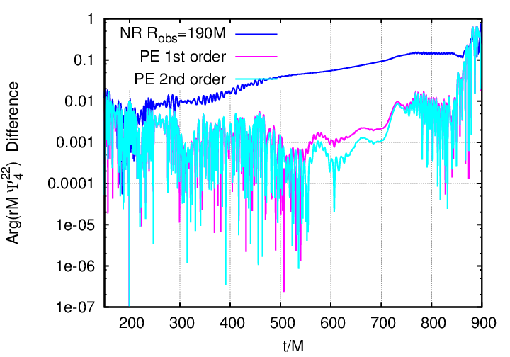
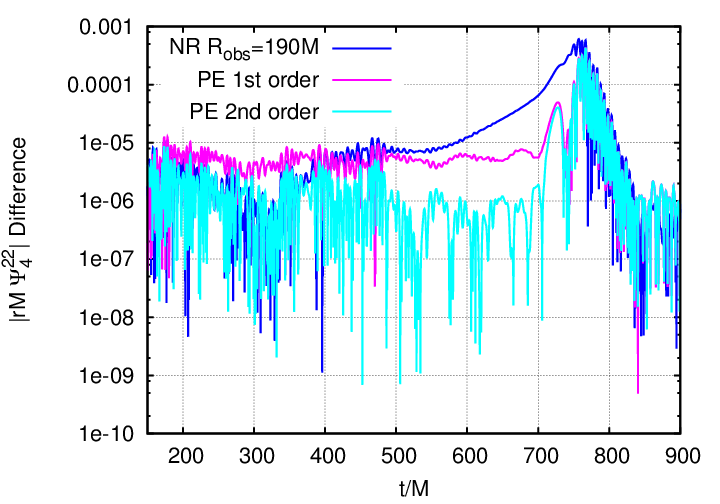
In order to produce a reference waveform that we may consider the best extrapolation and hence approximation to the exact waveform in Fig. 4, we took the highest resolution run and used the ten extraction radii we have to extrapolate the waveform in time using a 2nd order fitting polynomial in $1/r$ . We extrapolated the amplitude and phase after shifting the time by the tortoise radius for each extraction radius. We then can compare the amplitude and phase of this extrapolated waveform to a finite radius waveform ( $R_{\rm obs}=190M$ , our largest extraction radius), and to the waveforms produced by using the $1/r$ and $1/r^{2}$ order perturbative extrapolations (without the terms depending on the spin). The results are displayed in Fig. 5 which shows the benefits of using our formulas to approximate the waveform phase and amplitude at infinity. Note that given the different dependence of the phase correction ( $1/r$ as shown in Eq. (11)) and the amplitude correction ( $1/r^{2}$ as shown in Eq. (10)) the phase and amplitude show further improvements by including the second order corrections. This is more explicitly displayed in Fig. 6, that summarized the averaged differences.

VI Discussion

In this paper we describe a procedure for extrapolating the waveform at finite radius to infinity as a power series in $1/r$ . We provided the complete $1/r$ correction to the waveform in Eq. (49), including the spin terms in the background. We have also found it important to include the leading terms in $1/r^{2}$ in the extrapolation formula as given in Eq. (47). We have tested the extrapolation formula’s properties in a typical full numerical simulation of a black-hole binary, where we can verify the behavior of the extrapolation with different observer locations and finite-difference resolutions. In numerical simulations where the typical wavelength is relatively small compared to the boundaries of the simulation, the perturbative extraction provides at least a way of verifying the accuracy and consistency of the waveforms and radiative quantities such as the total energy and linear and angular momenta. In situations where it is extremely costly or inaccurate to extract at distances of two gravitational wavelengths from the sources (rule of thumb for the radiation zone), this method provides a crucial technique to evaluate waveforms and radiated quantities. In particular, we have seen that it is only the extrapolated waveform that converges with increasing resolution to the correct values and that extrapolation to infinite resolution of a finite extraction waveform can lead to a worse approximation. Although, for far enough location observer and resolution these two extrapolation processes eventually tend to commute.

The second order correction provided in Eq. (47) could be useful in situations where we have extended sources or one needs extreme resolutions near the sources and the simulation grid cannot reach the radiation zone. It also provides an independent way to estimate the errors of the first order extrapolation formula Eq. (49) by looking at the differences produced by these two extrapolation formulas.

Acknowledgements.

The authors gratefully acknowledge the NSF for financial support from Grants PHY-1305730, PHY-1212426, PHY-1229173, AST-1028087, PHY-0969855, OCI-0832606, and DRL-1136221. Computational resources were provided by XSEDE allocation TG-PHY060027N, and by NewHorizons and BlueSky Clusters at Rochester Institute of Technology, which were supported by NSF grant No. PHY-0722703, DMS-0820923, AST-1028087, and PHY-1229173. H.N. acknowledges support by the Grant-in-Aid for Scientific Research No. 24103006.

Appendix A Second order correction with $\psi_{0}^{\ell m}$

In Sub-Sec. II.2, the formula has a term, $\psi_{4}^{\ell m}$ integrated twice in time. In order to remove this term, we may use the identities in the Teukolsky formalism, and use the notation as given in Ref. [49]. In the Schwarzschild background with mass $M$ , the Weyl scalar $\psi_{4}$ and $\psi_{0}$ have following relations.

\displaystyle r^{4}\psi_{4}=\frac{1}{32}r^{4}f^{2}\left(\frac{1}{f}\partial_{t}-\partial_{r}\right)^{4}r^{4}f^{2}{\bar{\Psi}}\,,\quad\psi_{0}=\frac{1}{8}\left({\hbox to0.0pt{$\partial$\hss}\raise 3.00003pt\hbox{$-$}}^{4}{\bar{\Psi}}+12M\partial_{t}\Psi\right)\,,

(67)

where $f=1-2M/r$ and ${\hbox to0.0pt{$\partial$\hss}\raise 3.00003pt\hbox{$-$}}=-(\partial_{\theta}-s\cot\theta+i\csc\theta\partial_{\phi})$ for the spin-s weighted spherical harmonics [50]. $\Psi$ denotes a Hertz potential.

Here, since we are interested in the leading asymptotic behavior for large $r$ , the equation for $\psi_{4}$ is approximated as

\displaystyle r\psi_{4}

\displaystyle=

\displaystyle\frac{1}{32}{\cal T}^{4}r^{5}{\bar{\Psi}}\,,

(68)

where ${\cal T}=(\partial_{t}-\partial_{r}^{*})$ . In the above equation, the left hand side is written with respect to the retarded time $t-r^{*}$ . Therefore, using ${\cal T}^{-1}=(1/2)\int dt$ , we have

\displaystyle\int\int\int\int dt\,dt\,dt\,dt\,(r\psi_{4})

\displaystyle=

\displaystyle\frac{1}{2}r^{5}{\bar{\Psi}}\,.

(69)

For $\psi_{0}$ , we ignore the term proportional to $M$ in order not to introduce the complex conjugation of ${\bar{\Psi}}^{\ell m}$ , and focus on the term ${\hbox to0.0pt{$\partial$\hss}\raise 3.00003pt\hbox{$-$}}^{4}{\bar{\Psi}}$ . ${\bar{\Psi}}$ is a spin-( $-2$ ) function, i.e.,

\displaystyle\sum_{\ell m}\int\int\int\int dt\,dt\,dt\,dt\,(r\psi_{4}^{\ell m}){}_{-2}Y_{\ell m}

\displaystyle=

\displaystyle\frac{1}{2}r^{5}\sum_{\ell m}{\bar{\Psi}}^{\ell m}{}_{-2}Y_{\ell m}\,.

(70)

The operator $\partial$ $-$ on ${\bar{\Psi}}$ gives

\displaystyle{\hbox to0.0pt{$\partial$\hss}\raise 3.00003pt\hbox{$-$}}^{4}{\bar{\Psi}}=\sum_{\ell m}(\ell-1)\ell(\ell+1)(\ell+2){\bar{\Psi}}^{\ell m}{}_{2}Y_{\ell m}\,,

(71)

where there is no change in the $(t,\,r)$ dependence because $\partial$ $-$ acts only on the angular variables. Although there may be a relation between $12M\partial_{t}\Psi$ and the term proportional to $M$ in Eq. (75) below because both of the numerical factors are $3/2$ , we simply ignore it here in order not to introduce the complex conjugation of ${\bar{\Psi}}^{\ell m}$ . This means that we consider an approximation,

\displaystyle\sum_{\ell m}\psi_{0}^{\ell m}{}_{2}Y_{\ell m}

\displaystyle=

\displaystyle\frac{1}{8}\sum_{\ell m}(\ell-1)\ell(\ell+1)(\ell+2){\bar{\Psi}}^{\ell m}{}_{2}Y_{\ell m}\,.

(72)

Combining Eqs. (70) and (72), we have for each $(\ell,\,m)$ mode

\displaystyle\frac{1}{8}(\ell-1)\ell(\ell+1)(\ell+2)\int\int\int\int dt\,dt\,dt\,dt\,(r\psi_{4}^{\ell m})

\displaystyle=

\displaystyle\frac{1}{2}r^{5}\psi_{0}^{\ell m}\,,

(73)

in the large $r$ limit and the above approximation. Therefore, Eq. (23) is rewritten as

	$\displaystyle\left.r\,\psi_{4}^{\ell m}\right\|_{r=\infty}$	$\displaystyle=$	$\displaystyle r\,\psi_{4}^{\ell m}(t,r)-\frac{(\ell-1)(\ell+2)}{2\,r}\int dt\,[r\,\psi_{4}^{\ell m}(t,r)]$		(74)
			$\displaystyle+\frac{(\ell^{2}+\ell-4)}{2\,\ell(\ell+1)\,r^{2}}\partial_{t}^{2}[r^{5}\,\psi_{0}^{\ell m}(t,r)]-\frac{3\,M}{2\,r^{2}}\int dt\,[r\,\psi_{4}^{\ell m}(t,r)]+{\cal O}(1/r^{3})\,.$		(75)

Here, we have used $\psi_{0}^{\ell m}(t,r)$ extracted at a finite radius because the error due to the use of finite extraction radii becomes higher order in the large $r$ expansion. Since we have used an approximation to derive Eq. (72), for consistency, the $M$ -dependent term should not be kept any more, i.e.,

	$\displaystyle\left.r\,\psi_{4}^{\ell m}\right\|_{r=\infty}$	$\displaystyle=$	$\displaystyle r\,\psi_{4}^{\ell m}(t,r)-\frac{(\ell-1)(\ell+2)}{2\,r}\int dt\,[r\,\psi_{4}^{\ell m}(t,r)]$		(76)
			$\displaystyle+\frac{(\ell^{2}+\ell-4)}{2\,\ell(\ell+1)\,r^{2}}\partial_{t}^{2}[r^{5}\,\psi_{0}^{\ell m}(t,r)]+\textrm{[higher}\,\,\textrm{order]}\,.$		(77)

This derivation is in an ideal situation where we have assumed that there is no contribution from the other Weyl scalars, the peeling theorem applies, and we have used a low frequency $M\omega$ approximation.

References

[1] A. M. Abrahams, L. Rezzolla, M. E. Rupright, A. Anderson, P. Anninos, T. W. Baumgarte, N. T. Bishop, S. R. Brandt, J. C. Browne, K. Camarda, M. W. Choptuik, G. B. Cook, R. R. Correll, C. R. Evans, L. S. Finn, G. C. Fox, R. Gómez, T. Haupt, M. F. Huq, L. E. Kidder, S. A. Klasky, P. Laguna, W. Landry, L. Lehner, J. Lenaghan, R. L. Marsa, J. Massó, R. A. Matzner, S. Mitra, P. Papadopoulos, M. Parashar, F. Saied, P. E. Saylor, M. A. Scheel, E. Seidel, S. L. Shapiro, D. Shoemaker, L. Smarr, B. Szilagyi, S. A. Teukolsky, M. H. P. M. van Putten, P. Walker, J. Winicour, and J. W. Y. Jr, Phys. Rev. Lett. 80, 1812 (1998), gr-qc/9709082 .
[2] J. Baker, B. Brügmann, M. Campanelli, and C. O. Lousto, Class. Quant. Grav. 17, L149 (2000), gr-qc/0003027 .
[3] J. Baker, B. Brügmann, M. Campanelli, C. O. Lousto, and R. Takahashi, Phys. Rev. Lett. 87, 121103 (2001), gr-qc/0102037 .
[4] J. G. Baker, M. Campanelli, and C. O. Lousto, Phys. Rev. D65, 044001 (2002a), arXiv:gr-qc/0104063 [gr-qc] .
[5] J. G. Baker, M. Campanelli, C. Lousto, and R. Takahashi, Phys. Rev. D65, 124012 (2002b), arXiv:astro-ph/0202469 [astro-ph] .
[6] J. G. Baker, M. Campanelli, C. O. Lousto, and R. Takahashi, Phys. Rev. D69, 027505 (2004), arXiv:astro-ph/0305287 .
[7] M. Campanelli, B. J. Kelly, and C. O. Lousto, Phys. Rev. D73, 064005 (2006a), arXiv:gr-qc/0510122 .
[8] F. Pretorius, Phys. Rev. Lett. 95, 121101 (2005), gr-qc/0507014 .
[9] M. Campanelli, C. O. Lousto, P. Marronetti, and Y. Zlochower, Phys. Rev. Lett. 96, 111101 (2006b), gr-qc/0511048 .
[10] J. G. Baker, J. Centrella, D.-I. Choi, M. Koppitz, and J. van Meter, Phys. Rev. Lett. 96, 111102 (2006), gr-qc/0511103 .
[11] M. A. Scheel et al., Phys. Rev. D74, 104006 (2006), gr-qc/0607056 .
[12] M. A. Scheel et al., Phys. Rev. D79, 024003 (2009), arXiv:0810.1767 [gr-qc] .
[13] E. Pazos, M. Tiglio, M. D. Duez, L. E. Kidder, and S. A. Teukolsky, Phys. Rev. D80, 024027 (2009), arXiv:0904.0493 [gr-qc] .
[14] D. Pollney, C. Reisswig, E. Schnetter, N. Dorband, and P. Diener, Phys. Rev. D83, 044045 (2011), arXiv:0910.3803 [gr-qc] .
[15] C. Reisswig, N. T. Bishop, D. Pollney, and B. Szilagyi, Class. Quant. Grav. 27, 075014 (2010), arXiv:0912.1285 [gr-qc] .
[16] M. Babiuc, B. Szilagyi, J. Winicour, and Y. Zlochower, Phys. Rev. D84, 044057 (2011), arXiv:1011.4223 [gr-qc] .
[17] N. W. Taylor, M. Boyle, C. Reisswig, M. A. Scheel, T. Chu, et al., Phys. Rev. D88, 124010 (2013), arXiv:1309.3605 [gr-qc] .
[18] A. Vano-Vinuales and S. Husa, (2014), arXiv:1412.4801 [gr-qc] .
[19] A. Vano-Vinuales, S. Husa, and D. Hilditch, (2014), arXiv:1412.3827 [gr-qc] .
[20] C. O. Lousto, H. Nakano, Y. Zlochower, and M. Campanelli, Phys. Rev. D82, 104057 (2010), arXiv:1008.4360 [gr-qc] .
[21] C. O. Lousto, Y. Zlochower, M. Dotti, and M. Volonteri, Phys. Rev. D85, 084015 (2012), arXiv:1201.1923 [gr-qc] .
[22] I. Hinder, A. Buonanno, M. Boyle, Z. B. Etienne, J. Healy, et al., Class. Quant. Grav. 31, 025012 (2014), arXiv:1307.5307 [gr-qc] .
[23] C. O. Lousto and Y. Zlochower, Phys. Rev. D88, 024001 (2013), arXiv:1304.3937 [gr-qc] .
[24] T. Damour, F. Guercilena, I. Hinder, S. Hopper, A. Nagar, et al., Phys. Rev. D89, 081503 (2014), arXiv:1402.7307 [gr-qc] .
[25] U. Sperhake, V. Cardoso, F. Pretorius, E. Berti, and J. A. Gonzalez, Phys. Rev. Lett. 101, 161101 (2008), arXiv:0806.1738 [gr-qc] .
[26] M. Zilhao, S. C. Noble, M. Campanelli, and Y. Zlochower, Phys. Rev. D91, 024034 (2015), arXiv:1409.4787 [gr-qc] .
[27] K. Kyutoku, M. Shibata, and K. Taniguchi, Phys. Rev. D90, 064006 (2014), arXiv:1405.6207 [gr-qc] .
[28] T. Regge and J. A. Wheeler, Phys. Rev. 108, 1063 (1957).
[29] F. J. Zerilli, Phys. Rev. D2, 2141 (1970).
[30] W. Kinnersley, J. Math. Phys. 10, 1195 (1969).
[31] T. Nakamura, K. Oohara, and Y. Kojima, Prog. Theor. Phys. Suppl. 90, 1 (1987).
[32] C. O. Lousto, Class. Quant. Grav. 22, S543 (2005a), gr-qc/0503001 .
[33] C. O. Lousto, Class. Quant. Grav. 22, S569 (2005b), gr-qc/0501088 .
[34] A. Nagar and L. Rezzolla, Class. Quant. Grav. 22, R167 (2005), arXiv:gr-qc/0502064 .
[35] S. A. Teukolsky, Astrophys. J. 185, 635 (1973).
[36] H. Nakano, (2015), arXiv:1501.02890 [gr-qc] .
[37] M. Hannam, S. Husa, U. Sperhake, B. Brugmann, and J. A. Gonzalez, Phys. Rev. D77, 044020 (2008), arXiv:0706.1305 [gr-qc] .
[38] M. Boyle and A. H. Mroue, Phys. Rev. D80, 124045 (2009), arXiv:0905.3177 [gr-qc] .
[39] P. A. Sundararajan, G. Khanna, and S. A. Hughes, Phys. Rev. D76, 104005 (2007), arXiv:gr-qc/0703028 [gr-qc] .
[40] L. M. Burko and S. A. Hughes, Phys. Rev. D82, 104029 (2010), arXiv:1007.4596 [gr-qc] .
[41] P. Ajith, M. Boyle, D. A. Brown, B. Brugmann, L. T. Buchman, et al., Class. Quant. Grav. 29, 124001 (2012), arXiv:1201.5319 [gr-qc] .
[42] H. Tagoshi, M. Shibata, T. Tanaka, and M. Sasaki, Phys. Rev. D54, 1439 (1996), arXiv:gr-qc/9603028 [gr-qc] .
[43] E. Berti and A. Klein, Phys. Rev. D90, 064012 (2014), arXiv:1408.1860 [gr-qc] .
[44] M. Campanelli and C. O. Lousto, Phys. Rev. D59, 124022 (1999), arXiv:gr-qc/9811019 [gr-qc] .
[45] M. Campanelli, C. O. Lousto, H. Nakano, and Y. Zlochower, Phys. Rev. D79, 084010 (2009), arXiv:0808.0713 [gr-qc] .
[46] C. Reisswig and D. Pollney, Class. Quant. Grav. 28, 195015 (2011), arXiv:1006.1632 [gr-qc] .
[47] O. Dreyer, B. Krishnan, D. Shoemaker, and E. Schnetter, Phys. Rev. D67, 024018 (2003), gr-qc/0206008 .
[48] B. Krishnan, C. O. Lousto, and Y. Zlochower, Phys. Rev. D76, 081501 (2007), arXiv:0707.0876 [gr-qc] .
[49] T. S. Keidl, A. G. Shah, J. L. Friedman, D.-H. Kim, and L. R. Price, Phys. Rev. D82, 124012 (2010), arXiv:1004.2276 [gr-qc] .
[50] J. N. Goldberg, A. J. MacFarlane, E. T. Newman, F. Rohrlich, and E. C. G. Sudarshan, J. Math. Phys. 8, 2155 (1967).