Approximation of the Scattering Amplitude using Nonsymmetric Saddle Point Matrices
Abstract
In this paper we examine iterative methods for solving the forward () and adjoint () systems of linear equations used to approximate the scattering amplitude, defined by . Based on an idea first proposed by Gene Golub, we use a conjugate gradient-like iteration for a nonsymmetric saddle point matrix that is constructed so as to have a real positive spectrum. Numerical experiments show that this method is more consistent than known methods for computing the scattering amplitude such as GLSQR or QMR. We then demonstrate that when combined with known preconditioning techniques, the proposed method exhibits more rapid convergence than state-of-the-art iterative methods for nonsymmetric systems.
Keywords:
nonsymmetric saddle point matrix , conjugate gradient method , scattering amplitude1 INTRODUCTION
1.1 The Scattering Amplitude Problem
The core objective of this paper is to design and implement an iterative method for the solution of a system where the coefficient matrix is large, sparse, and nonsymmetric. The proposed method should be more efficient and robust than existing methods for solving such systems. One application in which such a system arises is in the computation of the scattering amplitude. The scattering amplitude, in quantum physics, is the amplitude of the outgoing spherical wave relative to that of the incoming plane wave [7]. It is useful when it is of interest to know what is reflected when a radar wave is impinging on a certain object. The scattering amplitude can be computed by taking the inner product of the right hand side vector of the
| (1) |
and the solution x of the
| (2) |
Applications of the scattering amplitude come up in nuclear physics [1], quantum mechanics [14], and computational fluid dynamics (CFD) [4]. One particular application is in the design of stealth planes [1].
The scattering amplitude creates a relationship between the right hand side of the adjoint system and the solution to the forward system in signal processing. The field is determined from the signal in the system . Then the signal is received on an antenna characterized by the vector which is the right hand side of the adjoint system , and it is expressed as [7]. We are interested in efficiently approximating the scattering amplitude. It is informative to look at methods that other researchers have used to solve this problem, which will be discussed below.
The solution of the linear system (2) is important for many applications beyond the scattering amplitude, such as in the numerical solution of PDE with non-self-adjoint spatial differential operators. This solution can be obtained in many different ways, depending on the properties of the matrix . The factorization can be used to solve some problems with a symmetric matrix or a Cholesky factorization can be used if the matrix is also known to be positive definite [9]. However, for large, sparse systems, an iterative method is preferred. The conjugate gradient method is the preferred iterative method for a symmetric positive definite matrix [9]. However it is much more difficult to find this solution for a matrix that is not symmetric positive definite. In the case that we have a matrix that is not symmetric, we can use methods like the biconjugate gradient (BiCG) [3] and generalized minimal residual (GMRES) methods [17]. If we have a matrix that is symmetric but indefinite, SymmLQ [24, 19] is the iterative method of choice. Since the scattering amplitude depends on both the forward and adjoint problem, it makse sense to use methods that take both the forward and adjoint problems into account, like the quasi-minimal residual (QMR) [16] and generalized least squares residual (GLSQR) methods[25].
1.2 Approximation of the Scattering Amplitude
The method of this paper employs a conjugate gradient-like approach since, for large, sparse matrices, it is best to use an iterative approach, such as the conjugate gradient method [11] which is particularly effective for symmetric positive definite matrices. In particular, conjugate gradient has a very rapid convergence if is near the identity either in the sense of a low rank perturbation or in the sense of the norm. In [9] it is stated that
Theorem 1
If is an symmetric positive definite matrix and rank()= then the Hestenes-Stiefel conjugate gradient algorithm converges in at most steps.
Theorem 2
Suppose is symmetric positive definite and . If the Hestenes-Stiefel algorithm produces iterates and then
where .
It is also stated in [9] that the accuracy of is often better than this theorem predicts and that the conjugate gradient method converges very rapidly in the -norm if , where is the of , defined by
with and referring to the largest and smallest singular values, respectively.
Multiplying both sides of by yields the normal equations with a symmetric matrix that is also positive definite when is invertible. However, this approach is not conducive to solving the forward and adjoint problems simultaneously. Furthermore, a significant problem with using is that now the condition number in the two-norm is squared for . Since this increases the sensitivity of the matrix, possibly making it ill-conditioned, this paper explores an alternative approach. The idea is to transform the problems and into an equivalent system in which the matrix can be guaranteed to have real, positive eigenvalues, as well as eigenvectors that are in some sense orthogonal, which is then conducive to solution using a conjugate gradient-like iteration. It is not necessarily symmetry that we seek, but we will have symmetry with respect to some inner product. To this end, we use an idea first proposed by Gene Golub in [5], and consider a nonsymmetric saddle point matrix that has the form
As required by the definition of a nonsymmetric saddle point matrix, we assume that the matrix is symmetric positive definite. The goal is to choose so that we can guarantee has real, positive eigenvalues. In this paper we will introduce the nonsymmetric saddle point conjugate gradient (NspCG) method to solve a nonsymmetric, large, sparse linear system, which will then allow us to compute the scattering amplitude. We will also use ILU preconditioning with NspCG, which gives rapid convergence compared to existing methods for solving such systems.
This paper is organized as follows. In Section 2 we discuss the known methods for solving a large linear system with iterative approaches to compute the scattering amplitude such as Bidiagonalization or least squares QR (LSQR), quasi minimum residual (QMR), and block generalized LSQR (GLSQR). In Section 3 we will introduce the method of this paper, NspCG. Section 4 will include an analysis of the numerical results. The preconditioning techniques and results can be found in Section 5. The conclusions and discussion of possible future work will be given in Section 6.
2 Methods for Solving the Linear Systems of the Forward and Adjoint Problems
2.1 QMR approach
The QMR approach [16, 7] is based on the spectral decomposition ; also the basis of the QMR approach is the unsymmetric Lanczos [9, 18] process which generates two sequences
that are biorthogonal, meaning . We have the following relations:
| (3) | |||||
| (4) |
where the tridiagonal matrices
and
have block structures in which and are not necessarily symmetric.
The residual, , in each iteration can be expressed as
| (5) | |||||
with a choice of where and . We now have the quasi-residual Then we choose , where and . Then the adjoint residual is . The vectors and are the solutions of the least squares problems for minimizing and . So now the solutions can be defined as
| (6) | |||||
| (7) |
2.2 LSQR approach
In LSQR [7, 19], a truncated bidiagonalization is used in order to solve the forward and adjoint problems approximately. The bidiagonal factorization of is given by where and are orthogonal and is bidiagonal. Thus the forward and adjoint systems can be written as
| (8) |
| (9) |
Now we can solve (8) by solving the following two systems
| (10) | |||||
| (11) |
and we can solve (9) by solving
| (12) | |||||
| (13) |
We need to use the following recurrence relations in an iterative process to produce a bidiagonal matrix
| (14) | |||||
| (15) |
where and are matrices with orthonormal columns, and
Also we have that
| (16) | |||||
and
Because is bidiagonal, it follows that is symmetric and tridiagonal. It can be seen from (16) that (14) and (15) implicitly apply Lanczos iteration to . Now this iterative process can be used to obtain the approximate solution to the forward and adjoint systems. We define the residuals at step as
| (17) | |||||
| (18) |
where
The goal of the LSQR approach is to obtain an approximation that minimizes the norm of the residual. That is, the norm is minimized. When working with the forward and adjoint problems, this approach is limited due to the relationship between the starting vectors
The above relationship does not allow to be chosen independently.
2.3 Generalized LSQR (GLSQR)
The GSLQR method [7, 25] overcomes the disadvantages of the LSQR method by choosing starting vectors and independently where, for an initial guess of and , and It is based on the factorizations
| (19) | |||||
| (20) |
From the above we get that
| (21) | |||||
| (22) |
where the recursion coefficients , , , and are chosen to make and have orthonormal columns, which yields
| (23) | |||||
| (24) | |||||
| (25) | |||||
| (26) |
We can define and , where , and . Now we have that
The residuals can be expressed as follows
| (27) |
and
| (28) |
The solutions and are
| (29) | |||||
| (30) |
3 Iterative Methods for Nonsymmetric Saddle Point Matrices
The matrix , defined as follows
| (31) |
where is invertible and is a symmetric positive definite matrix, is an example of a nonsymmetric saddle point matrix. It can be shown that for all . To see this, we first let Then can be written as
Now, if we let for any nonzero vector , then, . since is symmetric positive definite, we have that , since r is nonzero due to being invertible. On the other hand, if we assume , then That is, whether is nonzero or not, .
3.1 Ensuring a Real Positive Spectrum
We want to choose so that the matrix has a real positive spectrum, so it is suitable for a conjugate gradient-like iteration [15]. To make this choice we need to first define
where is a polynomial of degree one in the form for and
The goal here is to determine if there exists a symmetric positive definite matrix with respect to which is symmetric, meaning that is -symmetric if .
Let us first define a generic nonsymmetric saddle point matrix
and then define . We can use the following results from [15] to determine how to obtain a real positive spectrum:
Lemma 3
Let the matrix
be conformally partitioned with . Then
(1) is -symmetric, i.e., , and for any polynomial ,
(2) is -symmetric, i.e., , and
(3) is -symmetric, i.e., .
Theorem 4
The symmetric matrix is positive definite if and only if
| (33) |
where and denote the smallest and largest eigenvalues, respectively, and
| (34) |
A sufficient condition that makes positive definite can be derived from the above theorem.
Corollary 5
The preceding results lead to a simple approach to determining whether is suitable for a conjugate gradient-like iteration [15].
Corollary 6
If there exists a so that is positive definite, then has a nonnegative real spectrum and a complete set of eigenvectors that are orthonormal with respect to the inner product defined by . In case has full rank, the spectrum of is real and positive.
Using the previous results from [15], we obtain a simple criterion for determining whether the matrix from (31) can be constructed in such a way as to satisfy the criterion in Corollary 6.
Theorem 7
Let be an invertible real matrix, and let be a symmetric positive definite matrix that satisfies
| (37) |
Then the matrix defined by
has real positive eigenvalues and eigenvectors that are orthogonal with respect to the inner product defined by . That is, the above selection of makes the matrix suitable for a conjugate gradient-like iteration.
Proof: We need to satisfy (33) with a proper selection of . Let
based on Corollary 5. Because of how is defined, satisfies
| (38) |
which means (33) is also satisfied. Now we need to choose so that (36) from Corollary 5 holds. We require
| (39) |
or
| (40) |
where is equal to the largest singular value of , . From the fact that is symmetric positive definite, we obtain
Therefore, (40) is satisfied if
| (41) |
or, equivalently, if (37) is satisfied.
It follows that the matrix satisfies the requirements to make be symmetric positive definite and that has a real, positive spectrum from Corollary 6. This result makes the matrix suitable for a conjugate gradient-like iteration, as will be described below.
3.2 The Case
Let be the SVD of , where
and . In the case for some scalar , the condition from Theorem 7 reduces to
| (42) |
We now study the eigensystem of . Let for , where . The form of from (31), with , yields
| (43) | |||||
| (44) |
for . Substituting (44) into (43) yields
| (45) |
Multiplying through by and applying (44), we obtain
It follows that each is a multiple of a left singular vector of , and is the square of the corresponding singular value. Furthermore, from (44), we find that is a multiple of a right singular vector of .
We conclude that the eigenvectors of are given by
| (46) |
with corresponding eigenvalues that satisfy the quadratic equation
| (47) |
It can be shown directly from (46) and (47) that these eigenvalues are real and positive, and the corresponding eigenvectors linearly independent, if and only if satisfies the weaker condition
| (48) |
which is consistent with the necessary and sufficient condition for to be positive definite given in Theorem 4.
3.3 Nonsymmetric Saddle Point Conjugate Gradient Method
Let be nonsymmetric. We will now introduce a Conjugate Gradient (CG) approach that solves the linear system by solving an equivalent system of the form , where
| (49) |
The matrix is also not symmetric; however, the spectrum is entirely contained in the right half of the complex plane, due to the fact that for all . In the preceding discussion, we established that if was chosen so as to satisfy the assumptions of Theorem 7, then is diagonalizable with real, positive eigenvalues. Furthermore, the bilinear form , where , is a proper inner product, as is symmetric positive definite. It follows that is -symmetric and -definite, meaning that for all , and for all .
Let the vectors and be defined by
| (50) |
where , , and is the scattering amplitude for given vectors and that represent the field and antenna, respectively. The following conjugate gradient method is based on a given inner product for solving the linear system .
We have the inner product matrix suggested by [15]. From [15], we see that this choice of gives a working CG from the following lemma.
Lemma 8
Suppose that the symmetric matrix is positive definite. Then Algorithm 3.1 is well defined for and , and (until convergence) the scalars and can be computed as
| (51) |
| (52) |
With this choice of inner product matrix, it can be shown that the residuals computed using the preceding algorithm are, in some sense, orthogonal.
Theorem 9
Each residual as defined in Algorithm 3.1 is orthogonal to all previous residuals with respect to ,i.e. , where .
Proof: We know that . Let be defined as in (51). Also, we know that all of the search directions are orthogonal, i.e. for . We want to show that . This will be shown by induction, where the base case that we need to establish is
| (53) |
To show this we use the definition of and the expression for the search directions in the above algorithm, . Now we have that
| (54) |
Reindexing the definition of the residual from the algorithm yields the following expression for
Substituting this into (54) gives
| (55) |
Rearranging the last term in (55) yields
because is symmetric, and we already know that the search directions are orthogonal with respect to . Now it is easy to see that the denominator in (55) and the last factor in the numerator cancel leaving
Now we need to show that each residual is orthogonal to all previous residuals. We will do this by showing , where . Our induction hypothesis is To show this, first shift the indices to get the expression
Rearranging the recurrence relation for the search directions yields
Using this expression for and we obtain
| (56) | |||||
where
by the induction hypothesis. Now we are left with
where both terms are 0 due to the orthogonality of the search directions.
4 Numerical Results
In this section, we will analyze the results from the methods described in this paper. These methods include QMR from Section 2.2, GLSQR from Section 2.3, and NspCG from Section 3.1. We have duplicated the results from [7] for GLSQR and QMR and will compare them against the results for our NspCG method.
We need to first define the following matrix, is our nonsymmetric saddle point matrix
4.1 Example 1
This example uses the matrix created by A=sprand(n,n,0.2)+speye(n) in Matlab where n=100. This creates a random sparse matrix, where 0.2 is the density of uniformly distributed nonzero entries, and adds this to the identity.
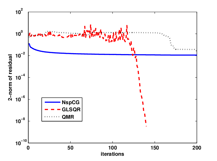
In Figure 1 we see that at the beginning of the iteration NspCG reaches a better approximation in fewer iterations than either QMR or GLSQR. Although GLSQR eventually outperforms NspCG, it takes about 120 iterations before it shows any sign of convergence at all. Then it converges rapidly.
4.2 Example 2
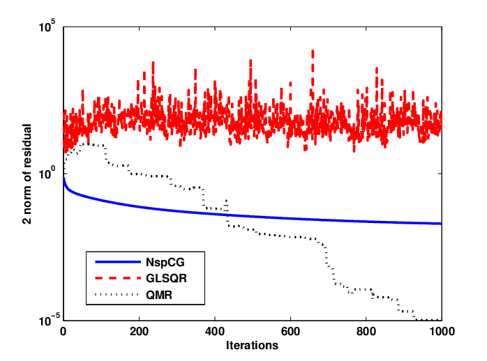
Example 2 uses the ORSIRR_1 matrix from the Matrix Market collection, which represents a linear system used in oil reservoir modeling. This matrix can be obtained from http://math.nist.gov/MatrixMarket/.
4.3 Example 3
First define the circulant matrix
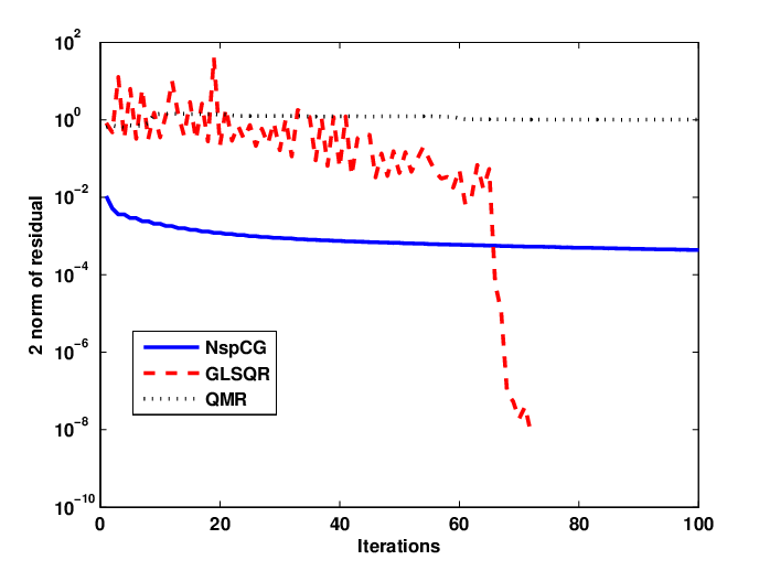
Now the matrix used in this example A=1e-3*sprand(n,n,0.2)+J, where n=100, can be constructed in Matlab.
4.4 Example 4
We need to first define
where and diag. Now we can define , where and are orthogonal matrices. For this example we use and .
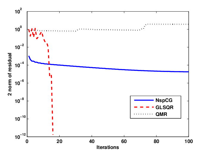
From 4 we see that NspCG starts off with the best approximation, but only for about 15 iterations. Then it is overtaken by GLSQR. Also, we can see that QMR fails to converge at all.
4.5 Example 5
This example uses the same definition of , , and from Example 4. In this example we will let again, and .
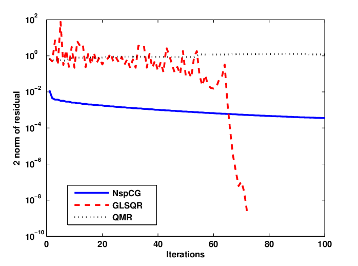
Figure 5 shows the same trend we have been seeing, that NspCG is more consistent at the beginning than any other method. At about 65 iterations GLSQR outperforms NspCG, and QMR fails to converge again.
4.6 Example 6
This example uses the same definition of , , and from Example 4. In this example we will let again, and .
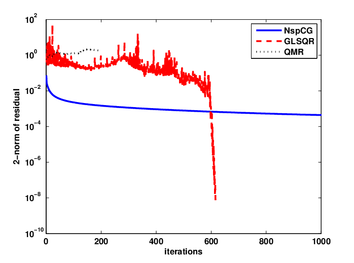
From Figure 6 we see that NspCG shows the best results for the first 600 iterations. GLSQR takes many iterations to converge in this case, and QMR does not converge at all.
5 Preconditioning
According to [9] conjugate gradient has very rapid convergence for a symmetric positive definite matrix that is nearly identity. We need to apply preconditioning techniques to make our matrix satisfy this criterion. The result will be that the original system is transformed into an equivalent system where the coefficient matrix is near identity. As we have seen previously with conjugate gradient, preconditioning techniques can be generalized to the nonsymmetric case. The goal is to apply preconditioning [23], while taking into account the structure of the nonsymmetric saddle point matrix . The matrix in the (1,1) block is assumed to be a symmetric positive definite matrix; therefore it has a Cholesky factorization . We can use the factorization
to obtain the factorization , where
| (57) |
Let us define
where an incomplete factorization [20] is computed from the sparse matrix which gives . By finding
| (58) |
it can be seen that the resulting preconditioned system matrix is given by
| (59) |
The above matrix has the structure similar to that of from (31), therefore it is a nonsymmetric saddle point matrix that is near .
5.1 Example 1
The following is Example 1 from the previous section with preconditioning.

5.2 Example 2
The following is Example 2 from the previous section with preconditioning.

In Figure 8 NspCG converges very rapidly in only 10 iterations. QMR takes over 200 iterations, but still doesn’t reach the level of accuracy that NspCG achieves. GLSQR does not converge at all.
6 Conclusions and Future Work
The results from this paper show that the NspCG method is much more consistent and reliable than GLSQR or QMR. NspCG only takes a few iterations to make fairly significant progress while GLSQR takes many iterations in most cases, and QMR rarely makes any progress. If preconditioning is used with NspCG, as is usually done with a conjugate gradient method, we have provided evidence that it will dramatically accelerate convergence, compared to state-of-the-art iterative methods such as GMRES or BiCG that are typically used to solve such systems. These results support our hypothesis that more rapid convergence can be achieved by solving a system that, while still nonsymmetric, shares essential properties with symmetric positive definite matrices and therefore is more suitable for conjugate gradient-like iteration.
Future work will include relating the NspCG method to a quadrature rule, as in [6, 10], that can be used to compute the scattering amplitude without explicitly solving the forward or adjoint problem. This has been done in [7] with the symmetric matrix
in conjunction with block Lanczos iteration [8], but our goal is to achieve more rapid convergence. Furthermore, because the forward system is replaced with a system with twice as many unknowns and equations, it is essential to implement the iteration carefully so that the gain in convergence speed is not offset by the additional expense of each iteration. To that end, it is worthwhile to consider other choices for the matrix instead of just a multiple of identity.
References
- [1] Arnett, D. Supernovae and Nucleosynthesis: An Investgation of the History of Matter, from the Big Bang to the Present, Princeton University Press, (1996).
- [2] Björck, A. "A Bidiagonalization Algorithm for Solving Ill-posed Sytem of Linear Equations". BIT, 41 (2001), pp. 659-670.
- [3] Brezinski, C., Redivo-Zaglia, M. "Look-Ahead in BiCGSTAB and Other Product-Type Methods for Linear Systems," BIT, 35 (1995), pp. 275-285.
- [4] Giles, M. B., Pierce, A. "An introduction to the adjoint approach to design", Flow, Turbulence, and Combustion, 65 (2000), pp. 393-415.
- [5] Golub, G. H., Lambers, J. V. Private communication, (November 6, 2007).
- [6] Golub, G. H., Meurant, G. "Matrices, Moments, and Quadrature". Proceedings of the 15th Dundee Conference, June-July (1993), Longman Scientific and Technical, (1994), pp. 105-156.
- [7] Golub, G. H., Stoll, M., Wathen, A. "Approximation of the Scattering Amplitude and Linear Systems". ETNA, 23 (2008), pp. 178-203.
- [8] Golub, G. H., Underwood, R. "The block Lanczos method for computing eigenvalues", Mathematical Software III, 7 (1977), pp. 361-377.
- [9] Golub, G. H., Van Loan, C.F.: Matrix Computations, The Johns Hopkins University Press (1996).
- [10] Golub, G. H., Welsch, J. "Calculation of Gauss Quadrature Rules" Math. Comp., 23 (1969), pp. 221-230.
- [11] Hestenes, M., Stiefel, E. "Methods of Conjugate Gradients for Solving Linear Systems" Journal of Research of the National Bureau of Standards 49(6) (1952).
- [12] Hnětynková, I., Strakoš, Z. "Lanczos Tridiagonalization and core problems". Linear Algebra Appl., 421 (2007), pp. 243-251.
- [13] Lambers, J. V. "Matrices, Moments, and Quadrature".
- [14] Landau, L. D., Lifshitz, E. Quantum Mechanics, Pergumon Press, Oxford, (1965).
- [15] Liesen, J., Parlett, B. "On Nonsymmetric Saddle Point Matrices that allow Conjugate Gradient Iterations". Numerische Mathematik, 108 (2008), pp. 605-624.
- [16] Lu, J., Darmofal, L. "A quasi-minimal residual method for simultaneous primal-dual solutions, and superconvergent functional estimates", SIAM J. Sci. Comput., 24 (2003), pp. 1693-1709.
- [17] Morgan, R.B. "A Restarted GMRES Method Augmented with Eigenvectors," SIAM J. Matrix Anal. Applic., 16 (1995), pp. 1154-1171.
- [18] Morgan, R. B. "On Restarting the Arnoldi Method for Large Nonsymmetric Egenvalue Problems", Math Comp., 65 (1996), pp. 1213-1230.
- [19] Paige, C. C., Saunders, M. A. "Algorithm 583 LSQR: Sparse Linear Equations and Least Squares Problems", ACM Trans. Math. Soft., 8 (1982b), pp. 195-209.
- [20] Papadopoulous, A.T., Duff, I. S., Wathen, A. J.: Incomplete Orthogonoal Factorization Methods Using Givens Rotations II: Implementation and Results BIT 45(1) (2005) 159-179.
- [21] Parlett, B. N., Nour-Omid, B. "The Use of a Refined Error Bound When Updating Eigenvalues of Tridiagonals", Lin. Alg. and it’s Applic, 34 (1980), pp. 31-48.
- [22] Parlett, B. N., Simon, H., Stringer, L. M., "On Estimating the Largest Eigenvalue with the Lanczos Algorithm", Math. Comp., 38 (1982), pp. 153-166.
- [23] Saad, Y.: Iterative methods for sparse linear systems. PSW (1996).
- [24] Saunders, M. A. "Solution of Sparse Rectangular Systems," BIT, 35 (1995), pp. 588-604.
- [25] Saunders, M. A., Simon, H.D., Yip, E. L. "Two conjugate-gradient-type methods for unsymmetric linear equations", SIAM J. Numer. Anal., 25 (1988), pp. 927-940.