Operational multipartite entanglement measures

Entanglement is of paramount importance in many fields of science. Due to its existence, applications such as teleportation, quantum computation, quantum simulation, and quantum error correction, to name a few, are feasible [1]. Moreover, the application of entanglement theory in other fields of science, most prominently condensed matter physics, has opened new routes towards the understanding of quantum many-body systems [2]. Due to its importance, an enormous effort has been made to qualify and quantify multipartite entanglement. Different entanglement classes have been identified and several entanglement measures have been introduced [3]. Some of them originated from analyzing the potentiality of a state for a particular realization of an application, such as the localizable entanglement [4], some others arose from the generalization of classical correlation measures, such as the generalization of the squashed entanglement [5, 3].

Despite these results, we are still far from completely understanding multipartite entanglement. The lack of knowledge stems on the one hand from the fact that the number of non-local parameters scales exponentially with the number of subsystems and, on the other hand, from the fact that the operations which are central in the investigation of entanglement, the local operations assisted by classical communication (LOCC), are notoriously difficult to be analyzed in general [6]. The importance of LOCC in this context is due to the fact that LOCC corresponds to those operations which can be implemented without consuming entanglement. This implies that entanglement is the resource to overcome the restriction to LOCC and that the sole condition a function has to fulfill to be a valid entanglement measure is that it is non-increasing under LOCC [3], ¹¹ 1 Note that sometimes entanglement quantifiers which are non-increasing on average under LOCC have been considered (see [3]).. For the bipartite case a simple criterion for pure state transformations via LOCC has been presented [7]. These results do not only allow to identify the state $\left|\Phi^{+}\right>\propto\sum_{i}\left|ii\right>$ as the maximally entangled state, which can be transformed into any other bipartite state deterministically via LOCC, but also allowed to introduce new entanglement measures. Due to the existence of different SLOCC classes in the multipartite setting [8, 9], i.e. the existence of pairs of states which cannot even probabilistically be transformed locally into each other, there does not exist a single state which is the optimal resource to overcome LOCC. This is why a set of states, the maximally entangled set (MES) of $n$ subsystems, $MES_{n}$, has to be considered [10]. It is the minimal set of states from which any fully-entangled $n$-partite state can be obtained via LOCC.

In order to quantify entanglement, possible LOCC transformations among multipartite states have to be further investigated with the intention to identify new operational entanglement measures. This is precisely the aim of this paper. We introduce operational entanglement measures for multipartite states (pure or mixed) of arbitrary dimensions ²² 2 Note that the fact that the measures are applicable for any dimension is crucial, as LOCC might increase the dimension of the considered Hilbert space.. As we are going to show, the measures can be easily computed whenever all possible LOCC transformations are known, as in the case of pure states describing few-partite systems [7, 11] ³³ 3 Note that the LOCC convertibility among mixed states is only partially known even in the case of bipartite systems [12].. The operational character of the new measures allows to prove very easily that they are indeed non-increasing under LOCC and admits a generalization to two classes of entanglement measures.

We outline how to compute the new measures for bipartite pure states of arbitrary dimensions. For pure three-qubit systems we derive explicit formulas for them and show that they, together with some well-known bipartite measures, allow us to completely characterize the entanglement contained in the state in an operational way. This characterization shows that the W- and GHZ-state are the most useful tripartite states regarding state manipulation.

Throughout this paper, $\sigma_{x},\sigma_{y},\sigma_{z}$ denote the Pauli operators and $1\hskip-2.84526pt{\bf l}$ the identity operator. When studying possible LOCC transformations we always consider representatives of Local Unitary (LU)-equivalence classes, as LUs do not alter the entanglement contained in a state and can obviously always be applied to a state. We say that a state $\left|\Psi\right>$ can reach a state $\left|\Phi\right>$ if there exists a LOCC protocol which transforms $\left|\Psi\right>$ into $\left|\Phi\right>$ (deterministically). In this case $\left|\Phi\right>$ is accessible from $\left|\Psi\right>$.

Let us now introduce the new operational entanglement measures. For a given state, $\left|\Psi\right>$, we denote by $M_{a}(\left|\Psi\right>)$ the set of states which can be accessed via LOCC from $\left|\Psi\right>$ and by $M_{s}(\left|\Psi\right>)$ the set of states which can reach $\left|\Psi\right>$. The following two magnitudes occur then naturally in the context of possible LOCC transformations: the source volume, $V_{s}(\left|\Psi\right>)=\mu[M_{s}(\left|\Psi\right>)]$, which measures the amount of states that can be used to reach the state $\left|\Psi\right>$ and the accessible volume, $V_{a}(\left|\Psi\right>)=\mu[M_{a}(\left|\Psi\right>)]$, which measures the amount of states that can be accessed by $\left|\Psi\right>$ via LOCC. Here, $\mu$ denotes an arbitrary measure in the set of LU equivalence classes. The underlying idea is that if a state $\left|\Psi\right>$ can be reached by many states, i.e. if $M_{s}(\left|\Psi\right>)$ is very large, then the state is not very powerful as any state in $M_{s}(\left|\Psi\right>)$ could be used for the same purpose and for possibly more applications. On the other hand, if the accessible set is very large the state is very valuable, as it can be used for any potential application of any state in $M_{a}(\left|\Psi\right>)$.

Due to the operational meaning of $M_{a}$ and $M_{s}$, it is easy to construct now operational entanglement measures. In order to do so we first show that $M_{a}$ ($M_{s}$) can only become smaller (larger) under LOCC, respectively. Consider a state $\left|\Psi\right>$ and any state $\left|\Phi\right>_{\Psi}$ which is accessible from $\left|\Psi\right>$ via LOCC. As any state in $M_{s}(\left|\Psi\right>)$ can first be transformed via LOCC into $\left|\Psi\right>$ and then to $\left|\Phi\right>_{\Psi}$, it is obvious that $M_{s}(\left|\Phi\right>_{\Psi})$ contains $M_{s}(\left|\Psi\right>)$. That $M_{a}(\left|\Phi\right>_{\Psi})\subseteq M_{a}(\left|\Psi\right>)$ can be easily verified noting that any state which can be reached from a state $\left|\Phi\right>_{\Psi}$ can in particular be reached from a state that can reach $\left|\Phi\right>_{\Psi}$. Hence, any properly normalized and rescaled measure of these sets is indeed an entanglement measure, i.e. it does not increase under LOCC. A possible choice would be $E_{a}(\left|\Psi\right>)=V_{a}(\left|\Psi\right>)/V_{a}^{sup}$ and $E_{s}(\left|\Psi\right>)=1-V_{s}(\left|\Psi\right>)/V_{s}^{sup}$, where $V_{a}^{sup}$ ($V_{s}^{sup}$) denote the maximally accessible (source) volume according to the measure $\mu$. Note that these operational entanglement measures are applicable to arbitrary multipartite systems of any dimension. Moreover, these are valid entanglement measures for mixed states. Note further, that $M_{s}(\left|\Psi\right>)=\emptyset$ (implying that $V_{s}(\left|\Psi\right>)=0$) iff the state $\left|\Psi\right>$ is in the MES, as these are the only states which cannot be reached by any other state [10]. We elaborate on how this measures can be computed in case of few-partite pure states below.

The notion of these entanglement measures can be generalized in the following way. Considering a $n$-partite state, $\left|\Psi\right>\in\hbox{$I$\kern-6.99997pt$C$}^{d_{1}}\otimes\cdots\otimes\hbox{$I$\kern-6.99997pt$C$}^{d_{n}}$, one can also measure its entanglement by (i) the amount of $(n-k)$-partite entangled states one can reach from $\left|\Psi\right>$, for $k\geq 1$, or (ii) by the amount of reachable states in $\hbox{$I$\kern-6.99997pt$C$}^{d^{\prime}_{1}}\otimes\cdots\otimes\hbox{$I$\kern-6.99997pt$C$}^{d^{\prime}_{n}}$, where at least one of the local dimensions, $d_{i}^{\prime}$, is reduced. Similarly, one can generalize the notion of the source volume to a whole class of entanglement measures by relating not only elements of the same Hilbert space.

We are going to use now these quantities and the previously obtained results on possible LOCC transformations [7, 11, 13] in order to quantify the entanglement contained in few-body pure states. Let us start by considering the bipartite case. We consider without loss of generality two $d$ level systems. It is well known that a state $\left|\Psi\right>$ can be transformed into a state $\left|\Phi\right>$ via LOCC iff $\lambda_{\Psi}$ is majorized by $\lambda_{\Phi}$, i.e $\lambda_{\Psi}\preceq\lambda_{\Phi}$, where $\lambda_{\Psi}$ denotes the vector containing the eigenvalues of the single party reduced state of $\left|\Psi\right>$ [7]. As the state is normalized, any vector $\lambda_{\Psi}$ belongs to a $d$-dimensional simplex. It has been shown that the set $S(y)=\{x\in\hbox{$I$\kern-6.00006pt$R$}^{d}|x\preceq y\}$ is the convex hull of $d!$ points obtained by permuting the components of $y$ [14]. Hence, in this parameter space and using the Lebesgue measure, the source and accessible volume of a state $\left|\Psi\right>$ are given by the volume of $S(\lambda_{\Psi})$ and $A(\lambda_{\Psi})=\{x\in\hbox{$I$\kern-6.00006pt$R$}^{d}|\lambda_{\Psi}\preceq x\}$ respectively (up to a constant factor, see [15]). In [15] we present closed formulas for $E_{s}$ and its generalization. Moreover, we present an algorithm to determine $E_{a}$ for arbitrary dimension and present explicit formulas for low dimensions, for which the new measures can be used to completely characterize the Schmidt coefficients.

Let us now present a complete characterization of entanglement of an arbitrary pure three-qubit state. In order to understand how the measures $E_{a}$ and $E_{s}$ are defined in this case we give a few remarks. First, we only consider the source and accessible volumes of genuinely entangled three-qubit states (i. e. we do not take into account biseparable states). Second, when we consider LOCC incomparable families of states such as the W and GHZ SLOCC classes, there is a freedom in choosing different measures $\mu_{1}$ and $\mu_{2}$ to compute the volumes for the different families without compromising the behaviour under LOCC of the entanglement measures. We exploit this freedom out of mathematical convenience. Last, even when considering LOCC comparable states, there exist states for which the corresponding source or accessible states are in manifolds of different dimensionality. Hence, if we use the same measure $\mu$ in both cases, this would assign a zero value to the accessible or source volumes of certain states even though they can indeed reach or be reached by other states, leading to a too coarse grained classification. Even though this would be a legitimate choice, we choose to use here a finer classification by choosing different measures to compute the volumes whenever the corresponding manifolds have different dimensions. Note that this choice, in contrast to the afore mentioned one, allows to compare the relative strength of states whose volumes have the same dimensionality. It should be clear however, that a state with e.g. a non-vanishing 4-dimensional accessible volume is infinitely more powerful than a state with a 3-dimensional accessible volume.

Up to LUs, any state in the W-class can be written as [10, 13]

where $x_{1},x_{2},x_{3}>0$, $x_{0}\geq 0$ and $\sum_{i=0}^{3}x_{i}=1$. Note that any state $\left|\Psi(\vec{x})\right>$ can be represented by the corresponding vector $\vec{x}=(x_{1},x_{2},x_{3})$ within a three-dimensional simplex $\mathcal{S}_{3}$ (see Fig. 1) [13]. As shown in [13], $\left|\Psi(\vec{x})\right>$ can be transformed into $\left|\Psi(\vec{y})\right>$ via LOCC iff $x_{i}\geq y_{i},\forall i\in\{1,2,3\}$. Due to that, it can be easily verified that the MES in the W-class, the W-MES, is the set of states with $x_{0}=0$. These states cannot be obtained from any other state, but any state in the W-class can be obtained from some state with $x_{0}=0$ [10].

Within the parameter space explained above, the accessible volume and the source volume of an arbitrary state $\left|\Psi(\vec{x})\right>$ can be easily shown to be (see also Fig. 1)

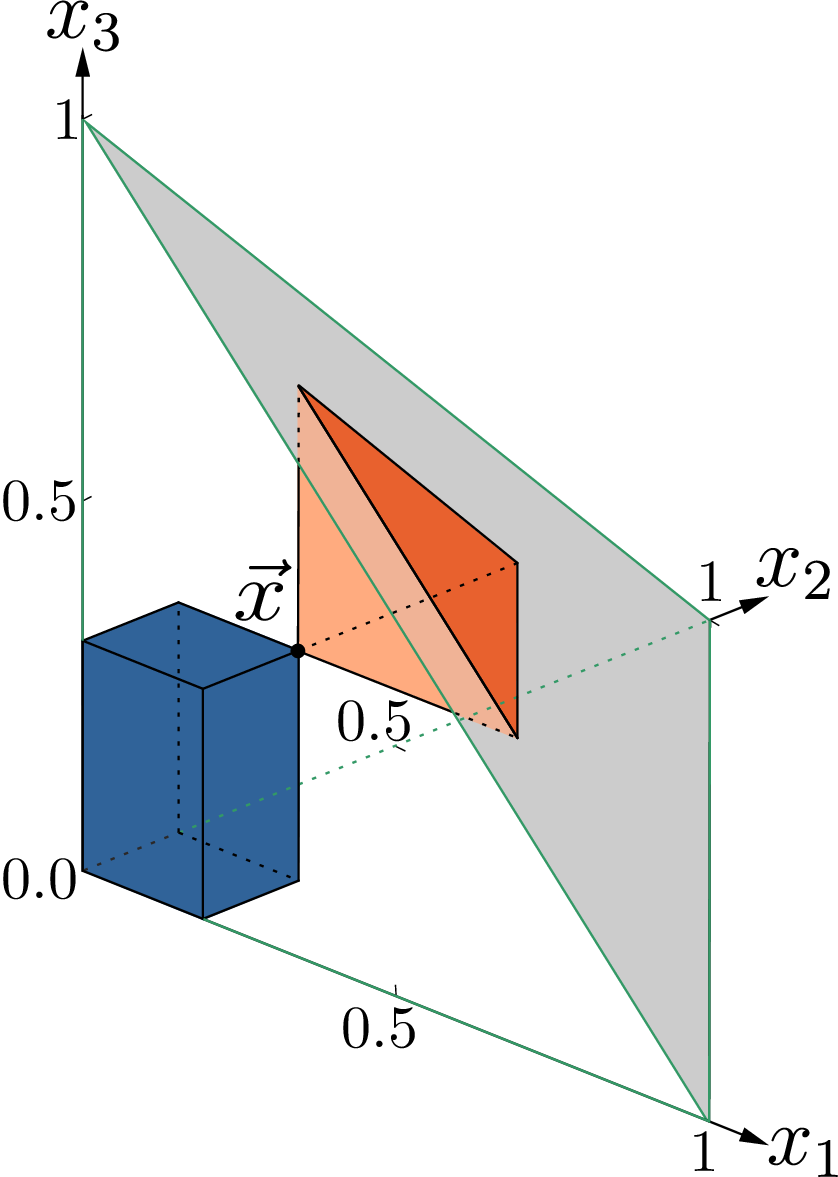
As mentioned above, it follows already from their definition that the corresponding measures, $E_{a}(\left|\Psi(\vec{x})\right>)=27V_{a}(\left|\Psi(\vec{x})\right>)$ and $E_{s}(\left|\Psi(\vec{x})\right>)=1-6V_{s}(\left|\Psi(\vec{x})\right>)$, are entanglement measures. A fact that can be particularly easily verified for the W-class using Eq. (2) and that no $x_{i}$ can be increased via LOCC. Note that the W-state maximizes both new measures, with $E_{a}(\left|W\right>)=1$ and $E_{s}(\left|W\right>)=1$. Hence, the W-state is the state that reaches the most other states deterministically via LOCC. It can therefore be regarded as the most useful state in the W-class.

Let us now characterize the entanglement contained in a state in the W-class. Due to the simplicity of this class, only bipartite entanglement measures, e.g. the three bipartite entanglement between party $i$ and the remaining parties, measured with e.g. the squared concurrence [16], $C_{i}(\left|\Psi(\vec{x})\right>)=4x_{i}(1-x_{i}-x_{0})$, are required to uniquely characterize the state (up to LUs). However, one could also employ the new measures and any of the bipartite measures for this purpose. In fact, as any three measures of the set $\{C_{1}(\left|\Psi\right>),C_{2}(\left|\Psi\right>),C_{3}(\left|\Psi\right>),E_{a}(\left|\Psi\right>),E_{s}(\left|\Psi\right>)\}$ are independent, we have that a state in the W-class is uniquely determined by any three of these operational entanglement measures.

Note that for any state in the W-MES it holds that $V_{s}(\left|\Psi(\vec{x})\right>)=0$. Moreover, for these states we have $C_{i}(\left|\Psi(\vec{x})\right>)=4x_{i}(1-x_{i})$. Hence, they can be easily characterized by any two of these bipartite measures or by any bipartite measure and $E_{a}(\left|\Psi(\vec{x})\right>)$. Note that the characterization via operational entanglement measures of arbitrary states in the W-class presented here can be easily generalized to $n$-qubit systems [15].

Let us now investigate the more complicated GHZ-class. A state in the GHZ-class can be written (up to LUs) as [10]

with $(g_{x}^{i})^{\dagger}g_{x}^{i}=\frac{1}{2}\mathbb{1}+g_{i}\sigma_{x},$ $g_{i}\in[0,1/2)$ $\forall i$, $\bm{g}=(g_{1},g_{2},g_{3})$, $P_{z}=diag(z,1/z),\ z\in\mathbb{C}$ with $|z|\leq 1$. As shown in [10], a state is in GHZ-MES iff $z=1$ or $z=i$ and either non of the $g_{i}$’s vanishes or all of them vanish, corresponding to the GHZ-state.

In [11] the necessary and sufficient conditions for the existence of a LOCC transformation from a state $\left|\Psi(\bm{g},z)\right>$ to another state $\left|\Psi(\bm{h},z^{\prime})\right>$ were obtained. As shown there, the absolute value of $z$ can be changed by LOCC independently of the other parameters only if at least one of the parameters $g_{i}$ vanishes, in which case $|z|$ can be arbitrarily decreased. As in this case different LOCC transformations are possible, we treat the cases (A) $g_{i}\neq 0$ for all $i$ and (B) at least one of the parameters $g_{i}$ vanishes separately.

Let us first consider case (A). Expressing the conditions for the existence of a LOCC transformation [11] from $\left|\Psi(\bm{g},z)\right>$ to $\left|\Psi(\bm{h},z^{\prime})\right>$ (see Eq. (3)) we obtain

1. (i)

   $g_{i}\leq h_{i}\ \ \forall i,$

2. (ii)

   $\displaystyle{\frac{g_{1}g_{2}g_{3}}{h_{1}h_{2}h_{3}}=\frac{\operatorname{Re}(z^{\prime 2})}{\left|z^{\prime}\right|^{4}+1}\frac{\left|z\right|^{4}+1}{\operatorname{Re}(z^{2})}=\frac{\operatorname{Im}(z^{\prime 2})}{\left|z^{\prime}\right|^{4}-1}\frac{\left|z\right|^{4}-1}{\operatorname{Im}(z^{2})}}$.

Note that cond. (ii) constitutes generically two independent equalities. However, in case the numerator and/or the denominator of one ratio vanishes, different conditions have to hold (see [17]).

We present now a characterization of the entanglement contained in an arbitrary state in the GHZ-class.

For this purpose we first consider states which are neither in GHZ-MES nor any $g_{i}$ vanishes, i.e. case (A) with $z\neq 1,i$. The other cases are treated below. The accessible and the source volume are given by (see [17])

with $f_{z}=\frac{2\left|\operatorname{Re}(z^{2})\right|}{1+\left|z\right|^{4}}$ and $G=g_{1}g_{2}g_{3}$ (see Fig. 2).

We show in [17] that $E_{a}(\left|\Psi(\bm{g},z)\right>)=8V_{a}(\left|\Psi(\bm{g},z)\right>)$ and $E_{s}(\left|\Psi(\bm{g},z)\right>)=1-8V_{s}(\left|\Psi(\bm{g},z)\right>)$ together with the three bipartite entanglement measures and one additional bit, that provides information about a specific state in the source set, uniquely determine the five parameters $z=re^{i\phi},g_{1},g_{2},g_{3}$ and therefore uniquely characterize the entanglement of the states up to complex conjugation (taken with respect to the computational basis) and LUs ⁴⁴ 4 Note that complex conjugation of a state corresponds to a redefinition of the complex unit and can therefore not alter any operational entanglement measure [18], if one considers only the state of interest, $\left|\Psi\right>$. (see [17] for details).

In [17] we show that the states where at least one $g_{i}$ vanishes can be treated similarly and that there the entanglement of the states is uniquely determined by the five operational entanglement measures.

It remains to consider the states in GHZ-MES, which constitute a three parameter family. In this case only cond. (i) and the first equation in cond. (ii) have to be fulfilled, which implies that only one parameter of the accessible states is fixed via cond. (ii). Hence, for $\left|\Psi_{MES}\right>$, a state in $MES_{3}$, we obtain the four dimensional accessible volume

with $G=g_{1}g_{2}\left|g_{3}\right|,\ H=h_{1}h_{2}h_{3}$. Putting the lower limits in Eq. (6) to zero we find $V_{a}^{sup}=1/8$. As the GHZ-state fulfills $g_{i}=0\ \forall i$ we have $E_{a}(\left|GHZ\right>)=1$ and therefore the GHZ-state is the state which reaches the most other states deterministically. The entanglement of a state in GHZ-MES, for which $V_{s}(\left|\Psi_{MES}\right>)=0$, can be similarly easily characterized as it was possible in the W-class (see [17]).

In summary, we have introduced two novel classes of operational entanglement measures, which are applicable to arbitrary multipartite pure or mixed states. We then demonstrated how these measures can be computed for the simplest pure multipartite case (three qubits) and showed that they can be used to completely characterize the entanglement contained in a three-qubit state. In [15] the new measures and its generalizations are determined for the bipartite setting of low dimension and the four-qubit case. It would be interesting to develop further the analysis of LOCC convertibility among mixed states in order to compute our measures in this case. Besides that and further extensions of this approach (e. g. approximate LOCC transformations, multi-copy case), it would also be appealing to connect our measures with different quantum information protocols and condensed-matter phenomena, which we leave for future research.

References

- [1] S. Turgut, Y. Gül, and N.K. Pak, Phys. Rev. A 81, 012317 (2010).
- [2] B. Kraus, Phys. Rev. Lett. 104, 020504 (2010); Phys. Rev. A 82, 032121 (2010).
- [3] C. H. Bennett, S. Popescu, D. Rohrlich, J. A. Smolin, A.V. Thapliyal, Phys. Rev. A 63, 012307 (2001).