On 3-dimensional hyperbolic Coxeter pyramids
Abstract.
After classifying 3-dimensional hyperbolic Coxeter pyramids by means of elementary plane geometry, we calculate growth functions of corresponding Coxeter groups by using Steinberg formula and conclude that growth rates of them are always Perron numbers. We also calculate hyperbolic volumes of them and compare volumes with their growth rates. Finally we consider a geometric ordering of Coxeter pyramids comparable with their growth rates.
Key words and phrases:
Coxeter group; growth function; growth rate; Perron number2010 Mathematics Subject Classification
Primary 20F55, Secondary 20F651. Introduction
Let denote hyperbolic –space and its closure. A convex polyhedron of finite volume is called a Coxeter polyhedron if all its dihedral angles are submultiples of or .
Let be a discrete group generated by finitely many reflections in hyperplanes containing facets of a Coxeter polyhedron and denote by the set of generating reflections. Then we call a hyperbolic Coxeter group with respect to . Note that the Coxeter polyhedron itself is a fundamental domain of . For each generator , one has while two distinct elements satisfy either no relation or provide the relation for some integer . The first case arises if the corresponding mirrors admit a common perpendicular or intersect at the boundary of , while the second case arises if the mirrors intersect in .
For a pair of a hyperbolic Coxeter group and a finite set of generators , we can define the word length of with respect to by the smallest integer for which there exist such that . We assume that for the identity element . The growth series of is the formal power series where is the number of elements satisfying . Since is an infinite group, the growth rate of , satisfies since , where denotes the cardinality of . By means of the Cauchy–Hadamard formula, it turns to the condition for the radius of convergence of . Therefore is not only a formal power series but also an analytic function of on the disk . It is known to be of exponential growth [4] and its growth rate is an algebraic integer (cf. [2]).
In this paper, we classify Coxeter pyramids of finite volume in by using the elementary plane geometry; we reduce it to the problem of circles and rectangles in Euclidean plane by using the link of the apex of a pyramid in upper half space model (see Section 3.1). Note that Tumarkin [12] already classified all Coxeter pyramids of finite volume in by using a combinatorial idea. Then by means of our former result [7] essntially, we show that the growth rates of Coxeter pyramids in are Perron numbers, i.e., real algebraic integers all of whose conjugates have strictly smaller absolute values. We also calculate hyperbolic volumes of Coxeter pyramids and check that volumes are not proportional to growth rates. Finally we introduce a partial ordering among Coxeter pyramids by using inclusion relation and show that this ordering is promotional to growth rates.
The paper is organized as follows. In Section 2 after reviewing the upper half space model of –dimensional hyperbolic space and the link of a vertex of a convex polyhedron, we classify Coxeter pyramids in . In Section 3 we collect some basic results of the growth functions and growth rates of Coxeter groups and show that growth rates of Coxeter pyramids are always Perron numbers. In section 4 we calculate hyperbolic volumes of Coxeter pyramids and compare them with their growth rates. Finally, in Section 5 we introduce a geometric ordering of Coxeter pyramids comparable with their growth rates.
2. Coxeter pyramids and their classification
2.1. The hyperbolic –space and its isometry group
The Euclidean 3-space contains the the Euclidean plane
which defines the upper half space of
Then is a model of the hyperbolic –space, so called the upper half space model. Let us denote by the boundary at infinity of in the extended space , and the closure of in .
A subset is called a hyperplane of if it is a Euclidean hemisphere or halfplane orthogonal to . If we restrict the hyperbolic metric of to , then it is a model of the hyperbolic plane.
Any isometry of can be represented as a composition of reflections with respect to hyperplanes. Also extends to the boundary map of so that is a composition of reflections with respect to the boundaries of hyperplanes, i.e. Euclidean circles or lines in . This correspondence induces the isomorphism between the isometry group of and Möbius transformation group of the Riemann sphere after identifying with by . consists of and the reflection with respect to the real axis of , defined by . It should be remarked that contains isometries corresponding to rotations, delations centered at , the reflection with respect to the real axis of , and parallel translations of .
2.2. Convex polyhedra and their vertex links
A closed half space is defined by the closed domain of bounded by a hyperplane . We define a convex polyhedron as a closed domain of which can be written as the intersection of finitely many closed half spaces; (it is also called a finite-sided convex -polyhedron in in [9]):
In this presentation of , we assume that is a hyperbolic polygon of . is called a face of and is called the supporting plane of . The dihedral angle between two faces and is defined as follows: if the intersection of two supporting planes and is nonempty, let us choose a point and consider the outer-normal vectors of and with respect to starting from . Then the dihedral angle is defined by the real number satisfying
where denote the Euclidean inner product of . It is easy to see that this does not depend on the choice of the base point . If and are parallel, i.e. the closures of and in only intersect at a point on , we define the dihedral angle is equal to zero, while if and are ultra-parallel, i.e. the closures of and in never intersect, we do not define the dihedral angle.
If the intersection of two facets and of a convex polyhedron consists of a geodesic segment, it is called an edge of . If the intersection of more than two facets is a point, it is called a vertex of . If the closures of and in only intersect at a point on , it is called an ideal vertex of . It should be remarked that the hyperbolic volume of a non-compact convex polyhedron is finite if and only if the closures of in consists of itself and ideal vertices.
Let be the hyperbolic sphere of radius centered at . If we restrict the hyperbolic metric of to , then it is a model of the 2-dimensional spherical geometry. To analyse local geometry of at a vertex , it is useful to study a cut locus of by a hyperbolic sphere of small radius centered at which is called a vertex link of at :
Theorem 1.
(cf. [9, Theorem 6.4.1]) Let be a vertex of a convex polyhedron in and be a hyperbolic sphere of based at such that meets just the facets of incident with . Then the link of in is a spherical convex polygon in the hyperbolic sphere . If and are two facets of incident with , then and are adjacent facet of if and only if and are adjacent sides of . If and are adjacent facets of incident with , then the spherical dihedral angle between and in is equal to the hyperbolic dihedral angle between the supporting hyperplanes and in .
A horosphere of based at is defined by a Euclidean sphere in tangent to at when , or a Euclidean plane in parallel to when . If we restrict the hyperbolic metric of to , then it is a model of the Euclidean plane. Similar to the previous case, it is useful to study a cut locus of by a small horosphere centered at an ideal vertex which is also called an ideal vertex link of at to analyse local geometry of at :
Theorem 2.
(cf. [9, Theorem 6.4.5]) Let be an ideal vertex of a convex polyhedron in and be a horosphere of based at such that meets just the facets of incident with . Then the link of in is a Euclidean convex polygon in the horosphere . If and are two facets of incident with , then and are adjacent facet of if and only if and are adjacent sides of . If and are adjacent facets of incident with , then the Euclidean dihedral angle between and in is equal to the hyperbolic dihedral angle between the supporting hyperplanes and in .
By means of this theorem we can visualize of at as follows: for an ideal vertex , applying with to , we may assume that . Since the vertical projection
maps a horosphere isometrically onto the Euclidean plane , the vertex link can be realized as a Euclidean polygon of , which will be a key idea for us to classify Coxeter pyramids in the next section.
2.3. Coxeter pyramids and their classification
A convex polyhedron of finite volume in is called a Coxeter polyhedron if all its dihedral angles are submultiples of or . Any Coxeter polyhedron can be described by a Coxeter graph defined as follows. The nodes of a Coxeter graph correspond to facets of . Two nodes are joined by an –labeled edge if the corresponding dihedral angle is equal to or . By convention we omit labelings for and delete edges for . Nodes are connected by a bold edge when the corresponding facets are parallel in .
Let be a Coxeter pyramid, i.e. a Coxeter polyhedron with five facets consisting of one quadrangular base facet and four triangular side facets. We call the vertex of opposite to a base facet an apex of . Then the apex should be an ideal vertex of ; suppose that is in . Then by Theorem 1, the vertex link would be isometric to a spherical Coxeter quadrangle, which contradicts to the absence of spherical Coxeter quadrangles by means of Gauss-Bonnet formula. Therefore the apex belongs to and by Theorem 2, the ideal vertex link of is isometric to a Euclidean Coxeter quadrangle, that is, a Euclidean rectangle.
Applying isometries of , we will normalize a Coxeter pyramid as follows: we may assume that the apex is , the support plane of the base facet is the hemisphere of radius one centered at the origin of , and side facets are parallel to -axis or -axis of . The vertex link of the apex of is projected on by the vertical projection , and we call its image the projected link, which is a rectangle in the closed unit disk in , whose edges are parallel to -axis or -axis. Let us call each edge bounding the projected link and (see Fig. 2), and denote by and the corresponding hyperplanes of . And let us denote by the base facet. Then we have
| (1) |


Let us denote by the dihedral angle between the associated hyperplanes supporting the side facets and the hyperplane supporting the bace facet. Note that the Euclidean distance between the origin and the edge satisfies (see Fig. 2).
Applying isometries of which induce a rotation of centered at the origin or a reflection of with respect to a line through the origin, we may assume that the dihedral angles of a Coxeter pyramid, say , , , satisfy
| (2) |
Summarising,
Definition 1.
A Coxeter pyramid is called normalized if
- •
the apex of is .
- •
The support plane of the base facet is the hemisphere of radius one centered at the origin of .
- •
Side facets and are parallel to -axis while side facets and are parallel to -axis of .
It is easy to see that there is a unique normalized Coxeter pyramid in its isometry class.
Now we can classify Coxeter pyramids in terms of Coxeter graphs by means of conditions (1) and (2). It should be remarked that these graphs were first appeared in [12, Table 2].
Theorem 3.
Coxeter pyramids in can be classfied by Coxeter graphs in Fig. 3 up to isometry.

Proof..


3. The growth of Coxeter pyramids
3.1. Growth functions of Coxeter groups
From now on, we consider the growth series of a Coxeter group where is its natural set of generating reflections. In practice, the growth series , which is analytic on where is the radius of convergence of , extends to a rational function on by analytic continuation where are relatively prime. There are formulas due to Solomon and Steinberg to calculate the rational function from the Coxeter graph of ([10, 11]; see also [5]), and we call this rational function the growth function of .
Theorem 4.
(Solomon’s formula)
The growth function of an irreducible finite Coxeter group can be written as
where and
is the set of exponents of (see [5]).
We give explicitly the growth functions of irreducible finite Coxeter groups in Table 1 where we use the notation (see [5, 6]).
| Symbol | Exponents | |
|---|---|---|
| 1, |
Theorem 5.
(Steinberg’s formula)
For a Coxeter group ,
let us denote by the Coxeter subgroup of generated by a subset , and let its growth function be .
Set is finite . Then
3.2. Growth rates of Coxeter groups
It is known that growth rates of hyperbolic Coxeter groups are bigger than ([4]). The formulas of Solomon and Steinberg imply that , and hence means that . Therefore the growth rate becomes a real algebraic integer. If is the unique pole of on the circle , then is a real algebraic integer all of whose conjugates have strictly smaller absolute values. Such a real algebraic integer is called a Perron number.
For two and three–dimensional cocompact hyperbolic Coxeter groups (having compact fundamental polyhedra), Cannon–Wagreich and Parry showed that their growth rates are Salem numbers ([1, 8]), where a real algebraic integer is called a Salem number if is an algebraic conjugate of and all algebraic conjugates of other than and lie on the unit circle. It follows from the definition that a Salem number is a Perron number.
Kellerhals and Perren calculated the growth functions of all four–dimensional cocompact hyperbolic Coxeter groups with at most 6 generators and checked numerically that their growth rates are not Salem numbers anymore while they are Perron numbers ([6]).
For the noncompact case, Floyd proved that the growth rates of two–dimensional cofinte hyperbolic Coxeter groups are Pisot–Vijayaraghavan numbers, where a real algebraic integer is called a Pisot–Vijayaraghavan number if all algebraic conjugates of other than lie in the open unit disk ([3]). A Pisot–Vijayaraghavan number is also a Perron number by definition.
From these results for low-dimensional cases, Kellerhals and Perren conjectured that the growth rates of hyperbolic Coxeter groups are Perron numbers in general.
3.3. Calculation of the growth functions
Finding all finite Coxeter subgraphs of a Coxeter diagram for a Coxeter pyramid classified in the previous section, we can calculate growth functions of Coxeter pyramids by means of formulas due to Solomon and Steinberg. The denominator polynomials of growth functions of Coxeter pyramids are listed below, where represents the Coxeter graph in Fig. 3. In Table 2 we also collect all growth rates of Coxeter pyramids, which arise as the inverse of the smallest positive roots of denominator polynomials of the growth functions.
- (1)
- (2)
- (3)
- (4)
- (5)
- (6)
- (7)
- (8)
- (9)
- (10)
- (11)
- (12)
- (13)
- (14)
- (15)
- (16)
- (17)
- (18)
- (19)
- (20)
- (21)
- (22)
- (23)
- (24)
- (25)
- (26)
- (27)
- (28)
- (29)
- (30)
- (31)
- (32)
- (33)
3.4. Arithmetic property of growth rates
Now we state the main theorem for growth rates of Coxeter pyramids.
Theorem 6.
The growth rates of Coxeter pyramids are Perron numbers.
Proof..
Let us denote the denominator polynomial of by . Then except 4 cases , , , and , has a form
where is a non-negative integer and the greatest common divisor of is . After multiplying by or , 4 exceptional cases also have this form:
In this case we already proved our claim in Lemma 1 of [7]; for the sake of readability, we recall its proof. Let us put . Observe , and is strictly monotonously increasing on the open interval . By the intermediate value theorem, there exists a unique real number in such that , that is, . Since all coefficients of the growth series are non-negative integers, is the radius of convergence of the growth series . Only we have to show is that has no zeros on the circle other than . Consider a complex number on the circle where is . If we assume , that is, ,
This implies that for all with . Now the assumption that the greatest common divisor of is equal to concludes that , hence is the unique pole of on the circle . ∎
4. The hyperbolic volumes of Coxeter pyramids
In this section, we calculate hyperbolic volumes of Coxeter pyramids by decomposing them into orthotetrahedra (cf. §10.4. of [9] ).
For this purpose, we use the projected link which we have introduced in the former section.
We express a Coxeter orthotetrahedron by the symbol
if its Coxeter graph is ![[Uncaptioned image]](1503.00583v1/orthotetra3.png) ,
and also express an ordinary orthotetrahedron by the same symbol where are not necessarily submultiples of .
,
and also express an ordinary orthotetrahedron by the same symbol where are not necessarily submultiples of .
First, let us consider the Coxeter orthopyramid whose Coxeter graph is linear (see the Coxeter graph in Fig. 7, where a bullet express the base facet). Note that its projected link is the rectangle on the first quadrant and its boundary (see the picture of a projected link in Fig. 7). Then, by the hyperplane passing through the apex , origin, and the vertex , is decomposed into two orthotetrahedra \footnotesize1⃝ and \footnotesize2⃝ with vertex , where (see the orthotetrahedra with corresponding numbers \footnotesize1⃝, \footnotesize2⃝ in Fig. 7). Note that we omit to write right angles in the pictures of Fig. 7.

The hyperbolic volume of each orthotetrahedron is calculated as follows (cf. [9, Theorem 10.4.6]) :
where denote Lobachevsky function defined by the formula of period (cf. [9, section 10.4]):
As a consequence, the hyperbolic volume of the orthopyramid is equal to the sum of volumes of two orthothterahedra:
Next, let us consider a Coxeter pyramid which is not an orthopyramid. By the hyperplanes each of which passes through the apex , origin and the vertex , where is one of the set , , and (see section 3.1), is decomposed into orthopyramids (see Fig. 8).

Then, decomposing each orthopyramid into two orthotetrahedra, we have a decomposition of into orthotetrahedra, and we can calculate the hyperbolic volume of . We collect hyperbolic volumes of all Coxeter pyramids in Table 2. We see that has the maximal volume among all Coxeter pyramids in . But we can say much more; by considering the normalization defined in Definition 1, any pyramid is contained in an ideal pyramid , i.e. a pyramid all of whose vertices are ideal. Then by means of Theorem 10.4.12 of [9], we can calculate the volume of . Moreover the proof of Theorem 10.4.11 of [9] implies that , the pyramid obtained by taking the cone to from an ideal square on the hemisphere of radius one centered at the origin of has the maximal volume among all ideal pyramids. Therefore
Theorem 7.
A pyramid of maximal volume in is .
It should be remarked that the order of growths is not equal to that of volumes; for example the growth of is smaller than that of while the volume of is bigger than that of .
| growth | volume | growth | volume | ||
|---|---|---|---|---|---|
| 2.40522 | |||||
| 2.41421 | |||||
| 1.9825 | 2.42032 | ||||
| 2.06599 | 2.45111 | ||||
| 2.06599 | 2.53983 | ||||
| 2.01561 | 2.58553 | ||||
| 2.1946 | 2.60198 | ||||
| 2.23757 | 2.64822 | ||||
| 2.24692 | 2.65364 | ||||
| 2.26809 | 2.68684 | ||||
| 2.30482 | 2.70039 | ||||
| 2.30522 | 2.72275 | ||||
| 2.33081 | 2.73526 | ||||
| 2.34913 | 2.74738 | ||||
| 2.35204 | 2.75303 | ||||
| 2.36644 | 2.84547 | ||||
| 2.38946 |
5. A geometric order of Coxeter pyramids comparable with their growth rates
We define a natural order of Coxeter pyramids in a geometric way. For Coxeter pyramids and , we define if there exists such that . It is easy to see that this binary relation is a partial order of the set of Coxeter pyramids. We also denote if corresponding Coxeter pyramids satisfy . We explain this geometric order in terms of appeared in section 2.3.
We study the relationship between this partial order and the growth rates of reflection groups. First, we shall state the following lemma which makes us to get back this order of reflection groups to that of the projected links of the apex of their fundamental Coxeter pyramids.
Lemma 1.
Let and be Coxeter groups defined by Coxeter pyramids. Then if and only if there exist corresponding Coxeter pyramids and with apex and bounded by a common hemisphere of radius centered at the origin, such that . Furthermore, the projected links and on of and satisfy in this case.
Proof..
As we have already seen in Section 2, there exists a Coxeter pyramid of transferred to have the apex and bounded by a common hemisphere of radius centered at the origin. Therefore by means of concurrency of the side facets of and , if and only if . ∎
Proposition 1.
For Coxeter groups and defined by Coxeter pyramids, if and only if there exist corresponding Coxeter pyramids and with numbering and described in Fig. 3 satisfying , , , and .
Proof..
It is obvious from concurrency of side facets passing through the apex . ∎
We describe the order relations of Coxeter pyramids in Fig. 9; each number represents the corresponding Coxeter pyramid and we attach its growth rate also. From this chart, we can see the following result.
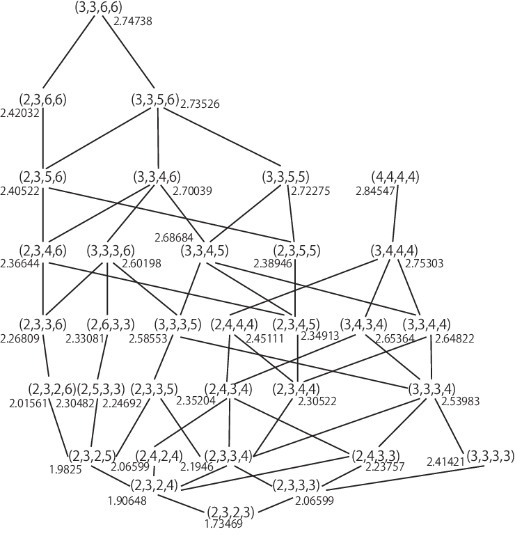
Corollary 1.
Let and be two Coxeter groups defined by Coxeter pyramids, and and be their growth rates respectively. Then if and only if .
Finally it shoud be remarked that the hyperbolic volume of the defining Coxeter pyramid of is smaller than or equal to that of if from the definition, while the converse is not true in general.
6. Acknowledgement
The authors thank Professor Ruth Kellerhals for telling them the reference [12]. The first author was partially supported by Grant-in-Aid for Scientific Research(C) (19540194), Ministry of Education, Science and Culture of Japan. The second author was partially supported by Grant-in-Aid for JSPS Fellows no. 12J04747, and by the JSPS Institutional Program for Young Researcher Overseas Visits “ Promoting international young researchers in mathematics and mathematical sciences led by OCAMI ”.
References
- [1] J. W. Cannon and Ph. Wagreich, Growth functions of surface groups, Math. Ann. 293 (1992), no. 2, 239–257.
- [2] M. W. Davis, The Geometry and Topology of Coxeter Groups, in: London Mathematical Society Monographs, Princeton University Press, 2008.
- [3] W. J. Floyd, Growth of planar Coxeter groups, P.V. numbers, and Salem numbers, Math. Ann. 293 (1992), no. 3, 475–483.
- [4] P. de la Harpe, Groupes de Coxeter infinis non affines, Exposition. Math 5 (1987), 91–96.
- [5] J. E. Humphreys, Reflection groups and Coxeter groups, Cambridge Studies in Advanced Mathematics, 29, Cambridge Univ. Press, Cambridge, 1990.
- [6] R. Kellerhals and G. Perren, On the growth of cocompact hyperbolic Coxeter groups, European J. Combin. 32 (2011), no. 8, 1299–1316.
- [7] Y. Komori and Y. Umemoto, Proc. Japan Acad. Ser. A Math. Sci. Volume 88, Number 4 (2012), 62–65.
- [8] W. Parry, Growth series of Coxeter groups and Salem numbers, J. Algebra 154 (1993), no. 2, 406–415.
- [9] J. G. Ratcliffe, Foundations of hyperbolic manifolds, Grad. Texts in Math., 149, Springer, New York, 1994.
- [10] L. Solomon, The orders of the finite Chevalley groups, J. Algebra 3(1966), 376–393.
- [11] R. Steinberg, Endomorphisms of linear algebraic groups, Memoirs of the American Mathematical Society, No. 80, Amer. Math. Soc., Providence, RI, 1968.
- [12] P. V. Tumarkin, Hyperbolic Coxeter n-polytopes with n+2 facets, Math. Notes 75 (2004), no. 5-6, 848–854. In Russian; translated in Russian Math. Surveys 40 (1985), 31–75.