Understanding nature from experimental observations: a theory independent test for gravitational decoherence
Abstract
Quantum mechanics and the theory of gravity are presently not compatible. A particular question is whether gravity causes decoherence - an unavoidable source of noise. Several models for gravitational decoherence have been proposed, not all of which can be described quantum mechanically [1, 2, 3]. In parallel, several experiments have been proposed to test some of these models [4, 5, 6], where the data obtained by such experiments is analyzed assuming quantum mechanics. Since we may need to modify quantum mechanics to account for gravity, however, one may question the validity of using quantum mechanics as a calculational tool to draw conclusions from experiments concerning gravity.
Here we propose an experiment to estimate gravitational decoherence whose conclusions hold even if quantum mechanics would need to be modified. We first establish a general information-theoretic notion of decoherence which reduces to the standard measure within quantum mechanics. Second, drawing on ideas from quantum information, we propose a very general experiment that allows us to obtain a quantitative estimate of decoherence of any physical process for any physical theory satisfying only very mild conditions. Finally, we propose a concrete experiment using optomechanics to estimate gravitational decoherence in any such theory, including quantum mechanics as a special case.
Our work raises the interesting question whether other properties of nature could similarly be established from experimental observations alone - that is, without already having a rather well formed theory of nature like quantum mechanics to make sense of experimental data.
Experiments aiming to test the presence - and amount - of gravitational decoherence generally go beyond established theory. Many theoretical models for gravitational decoherence have been proposed [3, 7, 8, 1, 9, 10, 11, 12, 13, 14, 15], and it is wide open if one of these proposals is correct. As such, experiments are of a highly exploratory nature, aiming to establish data points to which one may tailor future theoretical proposals. This task is made even more difficult by the fact that quantum mechanics and gravity do not go hand in hand, and indeed quantum mechanics may need to be modified in a yet unknown way in order to account for gravitational effects such as decoherence. We are thus compelled to design an experiment that provides a guiding light for the search for the right theoretical model - or indeed new physical theory - whose conclusions do not rely on quantum mechanics.
Decoherence in QM
As an easy warmup, let us first focus on the concept of decoherence within quantum mechanics. We first show how the protocol given in Figure 1 allows us to estimate quantum mechanical decoherence without knowing the decoherence process, and without doing quantum tomography to determine it. Traditionally, the presence of decoherence within quantum mechanics is related to the change of state due to measurement and the ”collapse of the wavefunction”. There are two complimentary ways to view this based on unconditional and conditional states. Given some pure quantum state, , and an arbitrarily accurate measurement of the variable diagonal in this basis, the post-measurement conditional states are or conditioned on the measurement outcome. On the other hand if this measurement has taken place but the results are unknown, the resulting unconditional state is given by the a quantum density matrix . The vanishing of the off-diagonal matrix elements in the measurement basis for the post measurement unconditional state forms decoherence. If the measurement is not arbitrarily accurate (i.e. weak) the off-diagonal matrix elements are reduced but do not vanish. More general forms of decoherence correspond to a decay of off-diagonal terms in the density operator with respect to any basis, and can occur due to the interaction of the system with an environment that may not be a measurement procedure of any kind. It is clear that this way of thinking about decoherence is entirely tied to the quantum mechanical matrix formalism, and also offers little in the way of quantifying the amount of decoherence in an operationally meaningful way.
The modern way of understanding decoherence in quantum mechanics in a quantitative way is provided by quantum information theory. One thereby thinks of a decoherence process as a interaction of a system with an environment as described in Figure 1, resulting in a quantum channel . The amount of of decoherence can now be quantified by the channel’s ability to transmit quantum information, i.e., its quantum capacity (see e.g. [16] and the appendix for further background). Concretely, one considers uses of the channel given by , and asks how many qubits we can send in relation to using an error-correcting encoding. Of particular interest is thereby the so-called single shot capacity, which determines the largest rate up to a given error parameter for any choice of 11 1 The asymptotic quantity often considered in information theory arises in the limit of , but the single-shot capacity gives more refined statements which are valid for any .. This single-shot capacity is determined by the so-called min-entropy [17, 18].
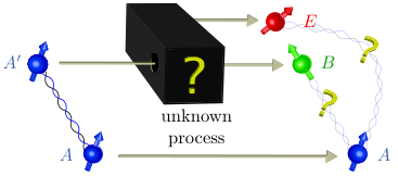
Apart from its information-theoretic significance, the min-entropy has a beautiful operational interpretation that also makes its role as a decoherence measure intuitively apparent. Very roughly, the amount of decoherence can be understood as a measure of how correlated becomes with . Suppose we start with a maximally entangled test state where the decoherence process is applied to . This results in a state (see Figure 1). If no decoherence occurs, the output state will be of the form where . That is, and are maximally entangled, but and are completely uncorrelated. The strongest decoherence, however, produces an output state of the form where and . That is, is now maximally entangled with , whereas and are completely uncorrelated. What about the intermediary regime? The min-entropy can be written as
| (1) |
where is the dimension of , and [19]
| (2) |
The maximization above is taken over all quantum operations on the system , which aim to bring the state as close as possible to the maximally entangled state . Intuitively, can thus be understood as a measure of how far the output is from the setting of maximum decoherence (where is the maximally entangled state). If there is no decoherence, we have giving and . If there is maximum decoherence, we have giving and where is simply the operation that discards the remainder of the environment . A larger value of thus corresponds to a larger amount of decoherence. In the quantum case, can be computed using any semi-definite programming solver [20, 21].
We hence see that in quantum mechanics, the relevant measure of decoherence is simply . How can we estimate it an experiment? Our goal in deriving this estimate will be to rely on concepts that we can later extend beyond the realm of quantum theory, deriving a universally valid test. It is clear that to estimate we need to make a statement about the entanglement between and - yet is inaccesible to our experiment. A property of quantum mechanics known as the monogamy of entanglement [22] nevertheless allows such an estimate: if is highly entangled, then is necessarily far from highly entangled. Since low entanglement in means that is low, a test that is able to detect entanglement between and should help us bound from above. We note that whereas any experimental proposal demands that we specifiy concrete measurements to be performed, our conclusions remain valid even if we do not have full control over the measurements, possibly because they are also somehow affected by an gravitational interaction in an unknown fashion. Dealing with unknown states and measurements is the essence of so-called device independence [23] in quantum cryptography. Allowing arbitrary measurements again forms a crucial stepping stone, enabling us to extend our results beyond quantum mechanics.
Beyond QM
The real challenge is to show that the conclusions of our test remain valid even outside of quantum mechanics. Since we want to make as few assumptions as possible, we consider the most general probabilistic theory, in which we are only given a set of possible states and measurements on these states. Every measurement is thereby a collection of effects satisfying and for all . We also refer to a measurement as an instrument . The label corresponds to a measurement outcome ’’. The notion of separated systems , and is in general difficult to define uniquely. We thus again make the most minimal assumption possible in which we identify ”systems” , and by sets of measurements that can be performed. For simplicitly, we take measurements and operations in the sets ,, and to commute, but do not impose any other strucuture. We thus merely use labels and and for commuting measurements. This means that for maps going from a system to an output system like the map is really from to and we use merely to remind ourselves we consider a restricted class of measurements on the output. Again, this is analogous to quantum mechanics where such measurements consist of operators on and the identity elsewhere (see appendix for a discussion).
The first obstacle consists of defining a general notion of decoherence. We saw that quantumly decoherence can be quantified by how well correlations between and are preserved, and this can be measured by how well the decoherence process preserves the maximally correlated state. Indeed, we can also quantify classical noise in terms of how well it preserves correlations, where the maximally correlated state takes on the form for some classical symbols . We hence start by defining the set of maximally correlated states, by observing a crucial and indeed defining property of the maximally correlated in quantum mechanics. Concretely, and are maximally entangled if and only if for any von Neumann measurement on , there exists a corresponding measurement on giving the same outcome. Again, the same is also true classically but made trivial by the fact that only one measurement is allowed. In analogy, we thus define the set of maximally correlated states as
| (3) |
This set coincides with the set of maximally entangled states in quantum mechanics, where can potentially contain an additional component in which is irrelevant to our discussion. We thus define
| (4) |
where is the state shared between and according to the general physical theory. The fidelity between two states and is thereby defined in full analogy to the quantum case [25] as
| (5) |
where the minimization is taken over all possible measurements , and denotes the probability distribution over the measurement outcomes of . That is, the fidelity can be expressed as the minimum fidelity between probability distributions of classical measurement outcomes. How about the transformation ? In general, it is difficult to characterize the set of allowed transformations in arbitrary physical theories, however we will not need make explicit in order to bound . Equation (4) gives us the familiar quantity within quantum mechanics, but provides us with an a very intuitive way to quantify decoherence in any physical theory that admits maximally correlated states. We emphasize that with our general techniques the latter demand could be weakend to allow all theories, even those who only have (weak) approximations of maximally correlated states. However, as we are not aware of any physically motivated example of such a theory, we leave such an extension to future study for clarity of exposition.
The second challenge is to prove that our test actually provides a bound on . Note that without quantum mechanics to guide us, all that we could reasonably establish by performing measurements on and are the probabilities of outcomes and given measurement settings and . That is, the probability
| (6) |
where and . Yet, given the system is entirely inaccessible to us we have no hope of measuring directly, where denotes a measurement setting on with outcome . Nevertheless, similar to quantum entanglement, it is known that no-signalling distributions are again monogamous [26] - and it is this fact that allows us to draw conclusions about by measuring only and . We will therefore make a non-trivial assumption about the physical theory, namely that no-signalling holds between , and . We emphasize weaker constraints on the amount of signalling could also lead to a bound - but we are not aware of any other concrete example to consider. Mathematically, no signalling means that the marginal distributions obey
| (7) |
that is, the choice of measurement settings and does not influence the distribution of the outcomes . A set of distributions is no-signalling if such conditions hold for all marginal distributions.
Abstract experiment
Our method is fully general and can in principle be used to measure the decoherence of any physical process. Figure 1 illustrates the general procedure. We create an entangled pair, and use half of this entangled pair to probe the unknown decoherence process. To estimate we will make use of the fact that in QM entanglement is monogamous, or more generally - when considering theories beyond QM - that no-signalling correlations are monogamous. This allow us to make statements about the correlations between and , even though we can only perform measurements on and . A test that allows us to bound from observations made on and alone is given by a Bell inequality [31, 32]. For the purpose of illustration, we consider creating an entangled state and perform a test based on the CHSH inequaltity [33] (see Figure 1). We emphasize that our methods are fully general and could be used in conjunction with other inequalities and higher dimensional entangled states.
As an easy warmup, let us first again consider what happens in quantum mechanics. For now, we assume that the measurement devices have no memory. That is, the experiment behaves the same in each round, independent on the previous measurements. It is relatively straight forward to obtain an upper bound on by extending techniques from quantum key distribution (QKD) [23]. In essence, we maximize over all states that are consistent with the observed CHSH correlator (see Figure 1). This maximization problem is simplified by the inherent symmetries of the CHSH inequality, allowing us to reduce this optimization problem to consider only states that are diagonal in the Bell basis. We proceed to establish properties of min and max entropies for Bell diagonal states, leading to an upper bound. Concretely, we show in the Appendix (Theorem B.1) that
| (8) |
where is an easy optimization problem that can be solved using Lagrange multipliers. We have chosen not to weaken this bound by an analytical bound that is strictly larger, as it is indeed easily evaluated (see Figure 3). If the devices are allowed memory, then a variant of this test and some more sophisticated techniques from QKD nevertheless can nevertheless be shown to give a bound.
How can we hope to attain an estimate outside of quantum mechanics? Let us first give a very loose intuition, why performing a Bell experiment on and , may allows us to bound . It is well known [26] that non-signalling correlations are also monogamous. That is, if we observe a violation of the CHSH inequality as captured by the measured parameter , then we know that the violation between and and also between and must be low. Note that the expectation values in terms of quantum observables and can be expresssed in terms of probabilities as
| (9) |
where we have again used in place of to remind ourselves that we may be outside of QM. In fact, if is larger than what a classical theory allows (), then and cannot violate the CHSH inequality at all. Let us now assume by contradiction that the state shared between and would be close to maximally correlated. Then by definition of the maximally correlated state, for every measurement on , there exists some measurement on which yields (almost) the same outcome. Hence, if would be close to maximally correlated, then we would expect that and can achieve a similar CHSH violation than and - because can make measurements that reproduce the same correlations that can achieve with . Yet, we know that this cannot be since CHSH correlations are monogamous.
In the appendix, we make this rough intuition precise. While we do not follow the steps suggested by this intuition, we employ a technique that has also been used for studying monogamy of CHSH correlations [26]. Specifically, we use linear programming as a technique to obtain bounds. We thereby first relate the fidelity to the statistical distance, which is a linear functional. We are then able to optimize this linear functional over probability distributions satisfying linear constraints. The first such constraint is given by the fact that we consider only no-signalling distribtions. The second by the fact that the marginal distribution leads to the observed Bell violation . The last one stems from the fact that maximal correlations can also be expressed using a linear constraint. Solving this linear program for an observed violation leads to Figure 3.
Optomechanics experiment
To gain insights into the significance of gravitational decoherence, we examine Diosi’s theory of gravitational decoherence [1]. This is equivalent to the decoherence model introduced in Kafri et al. [9]. It can be applied to an optomechanical cavity in which one mirror is free to move in a harmonic potential with frequency as in Figure 4. The master equation for a massive particle moving in a harmonic potential, including gravitational decoherence is
| (10) |
where
| (11) |
with the usual canonical position and momentum operators for the moving mirror. We have that
| (12) |
where the gravitational decoherence rate is given by
| (13) |
with the Newton gravitational constant and the density of the moving mirror. As one might expect is quite small, of the order of s-1 for suspended mirrors with . The term
| (14) |
with corresponds to mechanical heating. To see effect of the gravitational term stand out next to the mechanical heating we thus need to make the temperature low. A calculation shows that this model leads to a dephasing channel where is a function of the density , and the other parameters. In the appendix, we show that for this model
| (15) |
where is the Newton gravitational constant, is the Boltzman constant, and the Planck constant (see Figure 5 for the other parameters). (see Figure 5 for parameters)
Discussion
What have we actually learned when performing such an experiment? We first observe that the measured always gives an upper bound on the amount of decoherence observed - for any no-signalling theory. This means that even if quantum mechanics would indeed need to be modified we can still draw conclusions from the data we obtain. As such, the observations made in such an experiment establish a fundamental limit on decoherence no matter what the theory might actually look like in detail. It is clear, however, that the bound thus obtained is much weaker than if we had assumed quantum mechanics. No-signalling is but one of many principles obeyed by quantum mechanics, and these other features put stronger bounds on the values that can take. Our motivation for considering theories which are only constrained by no-signalling is to demonstrate even such weak demands still allow us to draw meaningful conclusions from such an experiment. One can easily adapt our approach by introducing further constraints on the probabilities - but not all of quantum mechanics - in order to get stronger bounds. In this case, one can similarly obtain an upper bound on from the measured data - this time for the more constrained theory. Also in a fully quantum mechanical world, our approach yields to a bound (see Figure 3). If we assume quantum mechanics, we may of course also try and perform process tomography in order to determine the decoherence process, and indeed any experiment should try and perform such a tomographic analysis whenever possible. The appeal of our approach is rather that we can draw conclusions from the experimental data while making only very minimal assumptions about the underlying physical theory.
One may wonder, why we only upper bound . Note that from our experimental statistics we can only make statements about the overall decoherence observed in the experiment, namely the gravitational decoherence (if it exists) as well as any other decoherence introduced due to experimental imperfections. Finding that the Bell violation is low (and thus maybe might be large) can thus not be attributed conclusively to the gravitational decoherence process, making a lower bound on meaningless if our desire is to make statements about a particular decoherence process such as gravity.
Second, we observe that our approach can rule out models of gravitational decoherence but not verify a particular one. It is important to note that a model for gravitational decoherence does not stand on its own, but is always part of a theory on what states, evolutions and measurements behave like. Given such a physical theory and a model for gravitational decoherence, we know enough to compute . In addition, we can compute an upper bound on specific to that theory, which may give a much stronger bound than no-signalling alone. Indeed, we see from Figure 3 that this is the case for quantum mechanics. Given the calculated and the experimentally observed value for , we can then compare: If , then the model (or indeed theory) we assumed must be wrong. However, if , then we know that the model and theory would be consistent with out experimental observations. We discuss this in more detail in the appendix with a candidate decoherence model that has been proposed and which - if it is valid - may be observed in the experiment suggested above.
Our approach thus provides a guiding light in the search for gravitational decoherence models. It is very general, and could in principle be used in conjunction with other proposed experimental setups and decoherence models. In particular, it could also be used to probe decoherence models conjectured to arise from decoherence affecting macroscopic objects, where there exist proposals to bring such objects into superposition [6]. Clearly, however, probing such models using entanglement is extremely challenging.
It is a very interesting open question to improve our analysis and to apply it to other physical theories that are more constrained than no-signalling, but yet do not quite yield quantum mechanics. Candidates for this may come from the study of generalized probabilistic theories where e.g. [36, 37, 38, 39, 40, 41] introduced further constraints in order to recover quantum mechanics, but also from suggested ways to modify the Schrödinger equation in order to account for non quantum mechanical noise. Since our approach could also be applied to higher dimensional systems, and other Bell inequalities, it is a very interesting open question whether other Bell inequalities could be used to obtain stronger bounds on from the resulting experimental observations.
Acknowledgements.
We thank Markus P. Müller, Matthew Pusey, Tobias Fritz and Gary Steele for insightful discussions. CP, JK, MT, AM, RS and SW were supported by MOE Tier 3A grant ”Randomness from quantum processes”, NRF CRP ”Space-based QKD”. SW was also supported by QuTech. NM and GM were supported by ARC Centre of Excellence for Engineered Quantum Systems, CE110001013References
- [1] L. Diósi, Phys. Rev. A 40, 1165 (1989).
- [2] R. Penrose, General Relativity and Gravitation 28, 581 (1996).
- [3] L. Diosi, J. Phys.: Conf. Ser. 306, 012006 (2011).
- [4] B. Pepper, R. Ghobadi, E. Jeffrey, C. Simon, and D. Bouwmeester, New J. Phys. 14, 115025 (2012).
- [5] W. Marshall, C. Simon, R. Penrose, and D. Bouwmeester, Phys. Rev. Lett. 91, 130401 (2003).
- [6] O. Romero-Isart, A. C. Pflanzer, F. Blaser, R. Kaltenbaek, N. Kiesel, M. Aspelmeyer, and J. I. Cirac, Phys. Rev. Lett. 107, 020405 (2011).
- [7] L. Diosi, Phys. Lett. A 105, 199 (1984).
- [8] L. Diosi, Phys. Lett. 120, 377 (1987).
- [9] D. Kafri, J. M. Taylor, and G. J. Milburn, New J. Phys. 16, 065020 (2014).
- [10] C. Anastopoulous and B. L. Hu, Class. Quant. Grav. 30, 165007 (2013).
- [11] B. L. Hu, Journal of Physics: Conference Series 504, 012021 (2014).
- [12] C. Anastopoulous and B. L. Hu, Journal of Physics: Conference Series 67, 012012 (2007).
- [13] B. Kay, Class. Quant. Grav. 15, L89 (1998).
- [14] H. P. Breuer, E. Göklü, and C. Lämmerzah, Class. Quant. Grav. 26, 105012 (2007).
- [15] C. Wang, R. Bingham, and J. T. Mendoca, Class. Quant. Grav. 23, L59 (2006).
- [16] M. Wilde, Quantum Information Theory (Cambridge University Press, 2013).
- [17] F. Dupuis, M. Berta, J. Wullschleger, and R. Renner (2010), arXiv:1012.6044.
- [18] F. Buscemi and N. Datta (2009), arXiv:0902.0158.
- [19] R. König, R. Renner, and C. Schaffner, IEEE Trans. Inf. Theory 55, 4337 (2009).
- [20] R. Renner, Ph.D. thesis, ETH Zürich (2005).
- [21] J. Sturm and AdvOL, http://sedumi.mcmaster.ca/.
- [22] B. Terhal, IBM Journal of Research and Development 48, 71 (2004).
- [23] A. Acín, N. Brunner, N. Gisin, S. Massar, S. Pironio, and V. Scarani, Phys. Rev. Lett. 98, 230501 (2007).
- [24] R. Horodecki, P. Horodecki, and M. Horodecki, Phys. Lett. A 200, 340 (1995a).
- [25] M. A. Nielsen and I. L. Chuang, Quantum Computation and Quantum Information (Cambridge University Press, 2000).
- [26] B. Toner, Proc. R. Soc. A 465, 59 (2009).
- [27] S. Popescu and D. Rohrlich, Phys. Lett. A 166, 293 (1992a).
- [28] S. Popescu and D. Rohrlich, Phys. Lett. A 169, 411 (1992b).
- [29] S. Popescu, Phys. Rev. Lett. 74, 2619 (1995).
- [30] S. Popescu, Phys. Rev. Lett. 72, 797 (1994).
- [31] J. Bell, Physics 1, 195 (1964).
- [32] N. Brunner, D. Cavalcanti, S. Pironio, V. Scarani, and S. Wehner, Rev. Mod. Phys 86, 419 (2014).
- [33] J. F. Clauser, M. A. Horne, A. Shimony, and R. A. Holt, Phys. Rev. Lett. 23, 880 (1969).
- [34] B. R. Nisbet-Jones, J. Dilley, D. Ljunggren, and A. Kuhn, New J. Phys. 13, 103036 (2011).
- [35] T. Kessler, C. Hagemann, C. Grebing, T. Legero, U. Sterr, F. Riehle, L. Martin, M. J. Chen, and J. Ye, Nature Photonics 6, 687 (2012).
- [36] L. Masanes and M. P. Müller, New J. Phys. 13, 063001 (2011), eprint 1004.1483, URL http://stacks.iop.org/1367-2630/13/i=6/a=063001.
- [37] L. Masanes, M. P. Müller, R. Augusiak, and D. Péréz-García (2012), eprint 1208.0493.
- [38] G. Chiribella, G. M. D’Ariano, and P. Perinotti, Phys. Rev. A 84, 012311 (2011), eprint 1011.6451, URL http://link.aps.org/doi/10.1103/PhysRevA.84.012311.
- [39] B. Dakic and C. Brukner, in Deep Beauty: Understanding the Quantum World through Mathematical Innovation, edited by H. Halvorson (Cambridge University Press, 2011), pp. 365–392.
- [40] C. Ududec, Ph.D. thesis, University of Waterloo (2012).
- [41] C. Pfister and S. Wehner, Nat. Commun. 4 (2013), eprint 1210.0194.
- [42] W. F. Stinespring, Proc. Amer. Math. Soc. 6 (1955).
- [43] B. Schumacher and M. A. Nielsen, Phys. Rev. A 54, 2629 (1996).
- [44] S. Lloyd, Phys. Rev. A 55, 1613 (1997).
- [45] P. Shor, The quantum channel capacity and coherent information (2002), URL http://www.msri.org/publications/ln/msri/2002/quantumcrypto/shor/1/.
- [46] I. Devetak, IEEE Trans. Inf. Theory 51, 44 (2005).
- [47] P. Hayden, M. Horodecki, J. Yard, and A. Winter, Open Systems and Information Dynamics 15, 7 (2008), quant-ph/0702005.
- [48] M. Tomamichel, R. Renner, and R. Colbeck, IEEE Trans. Inf. Theory 55, 5840 (2009).
- [49] V. Scarani and N. Gisin, Phys. Rev. Lett. 87, 117901 (2001), URL http://link.aps.org/doi/10.1103/PhysRevLett.87.117901.
- [50] R. Horodecki and M. Horodecki, Phys. Rev. A 54, 1838 (1996), ISSN 1050-2947, URL http://link.aps.org/doi/10.1103/PhysRevA.54.1838.
- [51] R. Horodecki, P. Horodecki, and M. Horodecki, Phys. Lett. A 200, 340 (1995b).
- [52] M. Tomamichel, Ph.D. thesis, ETH Zürich (2012).
- [53] A. Vitanov, F. Dupuis, M. Tomamichel, and R. Renner, IEEE Trans. Inf. Theory 59, 2603 (2013), ISSN 0018-9448, URL http://ieeexplore.ieee.org/lpdocs/epic03/wrapper.htm?arnumber=6408179.
- [54] G. W. Mackey, The mathematical foundations of quantum mechanics (W.A. Benjamin, 1093).
- [55] C. Edwards, Comm. Math. Phys. 16, 207 (1970).
- [56] E. B. Davies and J. T. Lewis, Commun. Math. Phys. 17, 239 (1970).
- [57] L. Hardy (2001), eprint quant-ph/0101012.
- [58] J. Barrett, Phys. Rev. A 75, 032304 (2007), eprint quant-ph/0508211, URL http://link.aps.org/doi/10.1103/PhysRevA.75.032304.
- [59] H. Barnum and A. Wilce (2009), eprint 0908.2354.
- [60] H. Barnum, J. Barrett, M. Leifer, and A. Wilce (2008), eprint 0805.3553.
- [61] H. Barnum, C. P. Gaebler, and A. Wilce (2009), eprint 0912.5532.
- [62] H. Barnum and A. Wilce, Electron. Notes Theor. Comput. Sci. 270, 3 (2011), ISSN 1571-0661, eprint 0908.2352, URL http://www.sciencedirect.com/science/article/pii/S157106611100003X.
- [63] C. Pfister (2012), eprint 1203.5622.
- [64] P. Janotta and R. Lal, Phys. Rev. A 87, 052131 (2013).
- [65] S. J. Summers and R. Werner, J. Math. Phys. 28, 2440 (1987).
- [66] V. B. Scholz and R. F. Werner (2008), eprint 0812.4305.
- [67] A. C. Doherty, Y.-C. Liang, B. Toner, and S. Wehner, Proc. 23rd IEEE Conf. on Computational Complexity (CCC’08) pp. 199–210 (2008).
- [68] C. H. Kraft, in University of California Publications in Statistics, Vol. 1 (University of California Press, 1955), pp. 125–142.
- [69] C. A. Fuchs and J. van de Graaf, IEEE Trans. Inf. Theory 45, 1216 (1999).
- [70] J. Barrett, N. Linden, S. Massar, S. Pironio, S. Popescu, and D. Roberts, Phys. Rev. A 71, 022101 (2005).
- [71] L.-M. Duan and C. Monroe, Rev. Mod. Phys. 82, 1209 (2010).
APPENDIX
Conventions
For this document, we make the following conventions.
- •
The logarithm is with respect to base 2, i.e. .
- •
Hilbert spaces are assumed to be finite-dimensional, unless otherwise stated.
- •
We denote the set of density operators (states) on a Hilbert space by .
- •
We identify operators on Hilbert spaces with their reordered versions resulting from permutations of systems. For example, for Hilbert spaces , , and states , , we identify the state with the state in resulting from the application of the braiding map on .
- •
For a state , we denote its reduced states by according changes of the subscript, e.g. , .
- •
For a state , entropies are evaluated for the according reduced states, e.g. is the conditional von Neumann entropy of (c.f. Section A.2).
Appendix A Background: Decoherence in quantum theory
In this section, we give a short introduction to decoherence in quantum theory. It consists of concepts, results and quantities that are well-established in quantum information science [16]. The topics are chosen to facilitate the understanding of our contributions in appendices B and C rather than to give a full introduction to the subject of decoherence. In Section A.1, we describe how the dynamical evolution of a system gives rise to a state of a tripartite system. This tripartite state plays a central role in our later analysis. In Section A.2, we explain why the min-entropy is the relevant quantity in the information theoretic analysis of decoherence. The min-entropy is the quantity that we use for our analysis in appendix B. It is also the quantity that serves as our motivation to define a decoherence quantity for generalized probabilistic theories in appendix C. We note that a generalization of quantum theory by, for example, introducing additional terms into the Schrödinger equation fall under the regime of generalized theories in our discussion.
A.1 Dynamical evolution and its tripartite purification
Interaction and non-unitary evolution: Suppose that a system , initially in a state described by a density operator , undergoes a dynamical evolution over some time interval. If undergoes this evolution as a closed system, then according to one of the postulates of quantum mechanics, the state transforms as
| (A.1) |
for a unitary (see Figure 6 (a)). In general, however, the system may be open, i.e. it may interact with another system that is called the environment. We consider the environment to consist of all the systems that interact with system . Taken together, the combined system then forms a closed system and hence evolves as
| (A.2) |
where is the initial state of the environment and is a unitary.
We may be ignorant about the environment and only have access to system . Our description would then treat the state of the subsystem after the evolution as a function of the state of before the evolution. We arrive at this description by taking the partial trace over in expression (A.2):
| (A.3) |
A map of the form (A.3) is easily shown to be a trace-preserving completely positive map (TPCPM). Thus, the evolution of an open system , when the environment is not visible, is described by a TPCPM (see Figure 6 (b)).
In a yet more general case, it may be that after the evolution of the system , we do not have access to system but to a different subsystem of . An example would be a two-particle system interacting with another two-particle system, where we only have access to one particle () of the four particles after the evolution. Mathematically speaking, the fact that we see a different subsystem before and after the evolution means that our factorization of the overall Hilbert space changes: Before the evolution, we write and after the evolution, we write (see Figure 6 (c)). Thus, the unitary evolution of the closed overall system is described by a unitary . Describing only the accessible part before and after the evolution, we end up with a TPCPM
| (A.4) |
Thus, the evolution of a system to a system , when being ignorant about the environment, is described by a TPCPM .
Stinespring dilation: We have demonstrated that unitaries on two (or more) systems give rise to TPCPMs on one system. It is well-known that the converse is also true: Every TPCPM can be extended to a unitary on a larger system in the following sense. For Hilbert spaces and of appropriate dimensions, it holds that for every pure state on , there is a unitary
| (A.5) |
such that
| (A.6) |
This (or an equivalent statement) is the Stinespring dilation theorem [42]. For more details see [16].
Textbook definitions of decoherence: From now on, we will take the viewpoint that the TPCPM is what we are given in the first place. Physically speaking, we assume that we are in the setting where all that we observe is a process in which a system in some state transforms into a state of some system . We think of this as a channel , into which we input a system and get a system as an output. Our goal in appendix A is to find a precise mathematical formulation of the following question in the quantum theoretical framework: How much does the channel decohere the system?
For the case where , the standard quantum mechanics literature gives some simple descriptions of what the decoherence of a system under a dynamical evolution is. As an example, consider the case where is a spin-1/2 particle, initially in the spin “up” state in the -direction,
| (A.7) |
If the channel is given by a measurement of the spin in the -direction, then, written in the -basis, the state of the system transforms as
One possible observation one can make in (A.1) is that the spin measurement in the -direction causes the off-diagonal terms of the density matrix to vanish. This is an extreme case of the dephasing channel in the -basis, which causes a loss of the phase information of the superposition (A.7). This loss of phase information is often equated with decoherence. Another feature of (A.1) that is often said to be the characteristic of decoherence is that turns an initially pure state into a mixed state.
These descriptions of decoherence, valid in their own right, are not favored by us for mainly three reasons. Firstly, these are no quantitative measures of decoherence. Secondly, they lack a clear operational meaning. Thirdly, they rely on the quantum mechanical formalism, in which states are expressed as density operators. It is not clear how to express them in more general cases that are not described by quantum theory.
In quantum information science, it is very popular to think of the systems arising in the purified picture we just presented as being controlled by parties with intentions and interests rather than just being dead physical objects. We will follow this spirit and from now on use the language of a game and speak of parties Alice, Bob and Eve, that we think of as agents controlling the systems , and .
A.2 The min-entropy as a measure for decoherence
The coherent information: As mentioned in Section A.1, it has been realized in quantum information science that important quantitative measures of the channel are functions of the state that we described above. One such measure quantifying decoherence is the coherent information [43]. It is defined in terms of the conditional von Neumann entropy
| (A.12) |
where and is the von Neumann entropy of the reduced state and , respectively. The coherent information is defined as
| (A.13) |
The coherent information has been shown to be related to the quantum channel capacity of , which is known as the Lloyd-Shor-Devetak (LSD) theorem [44, 45, 46]. It says that
| (A.14) |
where is the coherent information for and is a purification of . The state results from the -fold use of the channel to transmit , i.e. copies of system , while the purification of remains unchanged. Thus, the r.h.s. of (A.14) is the coherent information in the limit of infinitely many channel uses. Likewise, the quantum capacity is the limit of the achievable rate for quantum data transmission in the limit of infinitely many channel uses. One says that the quantum capacity, and therefore the coherent information, is an asymptotic quantity. This has the disadvantage that from the coherent information, only very limited statements about finitely many uses of the channel can be made.
The min-entropy: More insight about the behavior of the channel under finitely many uses can be gained by considering the corresponding single-shot quantity. To formulate it, note that the state is pure, in which case the duality relation for the conditional von Neumann entropy holds. This gives us
| (A.15) |
The corresponding single-shot quantity for the conditional von Neumann entropy is the conditional min-entropy, or just min-entropy, [20]. It is defined as
| (A.16) |
where the maximum is taken over all subnormalized density operators on , i.e. all positive operators on with trace between 0 and 1. The min-entropy quantifies the maximal size of a subsystem of that can be decoupled from [17], and thus tells us how many EPR pairs between Alice and Bob can be created [47] given a noisy output state . To obtain the single-shot capacity of channel uses we are - as in the asymptotic case - allowed to optimze over input states . Clearly, however, the resulting expression can be lower bounded using a particlar input state given by copies of the maximally entangled state. This is the test state we employ here, and hence our test also provides a bound on the single shot capacity. For instance if is a level system, then the min-entropy readily quantifies the number of EPR-pairs we can recover, given that we started with EPR pairs as an input. The min-entropy thus has a very appealing operational interpretation.
For our purposes, another expression for the min-entropy is more useful. In the following, we use the symbol to denote that two Hilbert spaces are isomorphic, i.e. means that the two spaces have the same dimension. It has been shown [19] that the min-entropy can be expressed as
| (A.17) |
where is the dimension of the Hilbert space of system , is a system with , the maximization is carried out over all TPCPMs from system to system , is the fidelity and is a maximally entangled state on , i.e. is an element of the set
| (A.18) |
The choice of , i.e. the choice of bases for and , is irrelevant for the value of . Since every is pure, we have that for any state on .
The expression (A.17) provides an intuition for the min-entropy. We think of the system , which is in the pure state , as being distributed between Alice, Bob and Eve. Imagine that Eve tries to perform operations on her share of the system with the intention to bring the reduced state between her and Alice as close as possible to the maximally entangled state , where the square of the fidelity is the measure of closeness. The closer Eve can bring the state to the maximally entangled state, the smaller the min-entropy . The overall situation of our decoherence analysis is shown in Figure 7.

The min-entropy is strictly more informative than the conditional von Neumann entropy in the following sense. In the iid limit (which stands for independent and identically distributed), where many identically prepared systems go through the channel and end up in a state , the min-entropy converges to the conditional von Neumann entropy:
| (A.19) |
where is an arbtirary smoothing parameter. This is known as the asymptotic equipartition property [48]. Thus, in the limit of infinitely many channel uses, where the asymptotic quantity is relevant, the min-entropy reproduces the conditional von Neumann entropy.
To gain some intuition for , we now have a look at some special cases. For these special cases, we assume that . Assume that initially, the state is maximally entangled, i.e. for some analogous to (A.18). We think of the channel purification as being controlled by Eve.
- •
If the adversary Eve leaves system untouched, i.e. the channel is the identity channel (or any other unitary channel), then for some state of system . In that case, , and we say that there is no decoherence.
- •
In the other extreme case, Eve snatches away the system and forwards an uncorrelated system to Bob. In this case, with analogous to equation A.18 (maximal entanglement between and ). Then, , and we say that we have full decoherence.
- •
As an intermediate case, we might consider the case where Eve interferes such that she does not end up with maximal entanglement with Alice but such that she is classically correlated with Alice in some basis, i.e. . In that case, , and we speak of partial decoherence.
Appendix B Decoherence estimation through CHSH tests in quantum theory
B.1 Introduction
Our goal is to show that Alice and Bob can estimate the decoherence by performing a Bell experiment. We pose it as a feasibility problem: is it possible to observe certain statistics in a Bell experiment given a certain level of decoherence? Solving this problem allows us to determine and plot the feasible region in the space of suitably chosen parameters.
We look at the simplest Bell experiment, known as the Clauser-Horne-Shimony-Holt (CHSH) [33] scenario. If is the state that Alice and Bob share and for are the observables they perform, then the CHSH value equals
| (B.1) |
As explained previously the min-entropy defined in Eq. (A.16) captures the notion of decoherence between Alice and Bob (although note that high min-entropy corresponds to low decoherence and vice versa). Since the range of values that the min-entropy takes depends on the dimension of Alice’s system (denoted by ), it is only meaningful to compare scenarios in which is fixed. For simplicity, we consider the simplest non-trivial scenario in which the subsystems held by Alice and Bob are qubits, .
We define the feasible region as follows. A pair of real numbers , where and belongs to if there exists a tripartite state and binary observables on and on such that
- •
subsystems and are qubits:
- •
The conditional min-entropy of given equals : .
- •
The CHSH value given by Eq. (B.1) equals : .
First note that a CHSH value of can be achieved using trivial measurements (namely ) acting on an arbitrary state. Therefore, for all values of are allowed. For the remainder of the argument we implicitly assume that and the following intuitive argument shows why certain pairs must indeed be forbidden. Consider a point and . According to the operational meaning of the min-entropy (A.17), means that Eve can recover the maximally entangled state with Alice with fidelity close to unity, which clearly allows Alice and Eve to violate the CHSH inequality. On the other hand, since Alice also observes a CHSH violation with Bob. This violates the monogamy relation for tripartite three-qubit states proved in Ref. [49], which states that Alice can violate the CHSH inequality with at most one party (even if she is allowed to use different measurements for different scenarios). This simple argument leads to the conclusion that the region and is forbidden. In the remainder of this section we show that the non-trivial part of the feasible region can be fully characterised by a single inequality.
Theorem B.1:
A pair of real numbers where and belongs to the feasible region if and only if
| (B.2) |
where
| (B.3) |
where the maximization is taken over
| (B.4) |
While the definition of might seem complicated, it is straightforward to see that is monotonically increasing in and evaluating numerically for a particular value of is straightforward since the function to be maximized is concave. The feasible region is plotted below.
![[Uncaptioned image]](1503.00577v1/hmin-region.png)
The proof of Theorem B.1 is conceptually simple, but it requires a wide array of technical tools, which we present in Section B.2. In Sections B.3 and B.4 we prove the direct and converse parts of Theorem B.1, respectively.
B.2 Preliminaries
Definition B.2:
Let , be Hilbert spaces of dimension . A generalized Bell basis for is a set of pure states on which satisfy
| (B.5) | ||||
| (B.6) |
A state is called Bell-diagonal if it is diagonal in some generalized Bell basis, i.e. if there exists a probability distribution such that
| (B.7) |
Lemma B.3:
Let be a positive semi-definite operator, let be the projector on its support and let be a normalised vector. Then iff
| (B.8) |
Note that since might not be invertible, is only defined on the support of .
B.2.1 Two-qubit states
A two-qubit state written in the Pauli basis takes the form
| (B.9) |
where all the summations go over . It is known that for every state there exists a local unitary which diagonalizes the correlation tensor (i.e. ensures that for ) and since all the properties we consider are invariant under local unitaries we can make this assumption without loss of generality. We denote these diagonal entries , and by and , respectively, which simplifies the expression to
| (B.10) |
Without loss of generality, we assume that and . As shown in Ref. [50] every Bell-diagonal state of two qubits (up to local unitaries which, again, we can safely ignore) can be written as
| (B.11) |
where is a probability distribution and and . It is easy to verify that
| (B.12) |
where
| (B.13) | ||||
B.2.2 Non-locality
Definition B.4:
For a bipartite quantum state the maximum CHSH value is defined as
| (B.14) |
where the maximisation is taken over all Hermitian, binary observables.
Note that for all states and we say that the state violates the CHSH inequality if . It was shown in Ref. [51] that if is a state of two qubits then the value of is fully determined by the correlation tensor. Adopting the convention we have
| (B.15) |
B.2.3 Entropic measures of entanglement
To derive a bound on the min-entropy , we will use a closely related quantity, namely the max-entropy.
Definition B.5:
For a bipartite quantum state the conditional max-entropy (or just max-entropy) is defined as
| (B.16) |
where is the maximally mixed state on and the maximisation is taken over all states on .
The proof uses the following known properties of the min- and max-entropies.
Lemma B.6 (Duality, [19]):
Let be a tripartite state. Then
and the equality holds iff is pure.
Lemma B.7 (Data-processing inequality, [20]):
For an arbitrary tripartite state we have
| (B.17) |
Lemma B.8 (Conditioning on classical information, Proposition 4.6 of [52]):
Let be a tripartite state where is a classical register:
| (B.18) |
Then
| (B.19) |
Finally, we need an explicit expression for the max-entropy of a Bell-diagonal state. Note that by assumption .
Lemma B.9:
Let be a Bell-diagonal state of form (B.7). Then the conditional max-entropy equals
| (B.20) |
To prove Lemma B.9 we use the fact that the optimization problem which appears in the definition of the max-entropy (B.16) can be written as a semidefinite program (SDP) [53]. More specifically, given we have , where is the value of the following SDP for being an arbitrary purification of
where denotes the set of positive semi-definite operators acting on . By providing feasible solutions for the PRIMAL and the DUAL we show that for Bell-diagonal states
| (B.21) |
which is precisely the statement of Lemma B.9.
Proof.
Let be a purification of , e.g.
| (B.22) |
For the PRIMAL consider
| (B.23) | |||
| (B.24) |
Clearly, , and since the first constraint is easy to check. The last inequality we need to check is
| (B.25) |
We apply Lemma B.3 to and . The projector on the support of equals
| (B.26) |
and it is easy to verify that . Moreover, since we have
| (B.27) | |||
| (B.28) |
Showing that and constitute a valid solution to the PRIMAL implies that .
For the DUAL consider
| (B.29) | |||
| (B.30) |
Note that is proportional to a rank-1 projector. The first constraint gives
| (B.31) |
and the remaining ones are easily verified to be true. The value of this solution equals which implies that . ∎
B.2.4 Sufficiency of considering Bell-diagonal states
To prove the converse part of Theorem B.1, we will use the following argument, which is similar in spirit and inspired by the symmetrization argument presented in Ref. [23].
Lemma B.10:
Let be an arbitrary state of two qubits. Then, there exists a Bell-diagonal state which satisfies
| (B.32) |
Proof.
We present an explicit construction of which meets the requirements. According to Eq. (B.10), can be written as
| (B.33) |
Moreover, consider the following random unitary channel
| (B.34) |
where , , and . It is easy to verify that for
| (B.35) |
because each Pauli operator commutes with identity and itself but anticommutes with the other two unitaries. This implies that is Bell-diagonal. Moreover, one can check that the map preserves the correlation tensor, i.e. for
| (B.36) |
which implies that . To check the last property consider the following state
| (B.37) |
By the data processing inequality, we have and by conditioning on classical information we have
| (B.38) | |||
| (B.39) |
Since the max-entropy is invariant under local unitaries we have for which implies that
| (B.40) |
∎
The final technical lemma concerns the problem of maximizing the max-entropy of a Bell-diagonal state of two qubits whose maximal CHSH violation is fixed.
Lemma B.11:
Let be a Bell-diagonal state of two qubits, whose maximal CHSH violation equals . Then, the max-entropy of satisfies the following inequality
| (B.41) |
for function defined in Eq. (B.3). Moreoever, there exists a state which saturates this inequality.
Proof.
According to Lemma B.9 the max-entropy of a Bell-diagonal state of two qubits equals
| (B.42) |
Here, it is convenient to express the probabilities through the correlation coefficients . Inverting Eqs. (B.13) gives
| (B.43) | |||
| (B.44) |
which allows us to write
| (B.45) |
where
| (B.46) |
In the space of correlation coefficients the feasible set are the triples for which the function is well-defined (the expressions under the roots must be non-negative). As before, we assume without loss of generality that and . Then, the maximal CHSH violation (we are only interested in states that violate the CHSH inequality) is given by Eq. (B.15)
Since in our case is fixed, the angular parametrisation takes the form
where and (which ensures ). Note that
It is easy to check that the allowed range of is
Note that we should also impose the condition but as it turns out the optimal solution will satisfy it even if we do not include it explicitly. To maximize the max-entropy it is sufficient to maximize function defined in Eq. (B.46), which in the angular parametrisation equals
| (B.47) |
over
| (B.48) |
The maximum is achieved either in the interior (denoted by ) or at the boundary. Let us start by ruling out the first option. Function is differentiable everywhere in and the partial derivatives are
| (B.49) | |||
| (B.50) |
To prove that there is no maximum in the interior, it suffices to show that there is no such that both derivatives vanish . To do this we consider the following linear combination
and show that has no solution in . Since the last term of is negative, a necessary condition for is that the sum of the first two terms is non-negative, which is equivalent to
This can be rearranged to give
which contradicts the second inequality in the definition of as shown below.
| (B.51) | |||
| (B.52) |
It is easy to check that the left-hand side of the final inequality is always at least , while the right hand side is always at most . This proves that the final (strict) inequality is always false, which implies that has no solutions in and that has no maximum in .
The boundaries and correspond to one of the expression under the roots being zero. Since the square root function has infinite slope at , such solutions cannot be optimal. Therefore, the maximum must be achieved at the boundary . Combining Equations (B.45) and (B.47) and setting leads directly to the statement of the lemma.
To show that the solution of the optimization problem satisfies , it is sufficient to show that for and the partial derivative is strictly positive. ∎
B.3 The direct part
Here, we show (by an explicit construction) that points described by and are allowed. Lemma B.11 shows that for there exists a Bell-diagonal state of two qubits whose max-entropy equals
| (B.53) |
By duality (Lemma B.6), if is an arbitrary purification, the conditional min-entropy equals
| (B.54) |
In this example , which corresponds to a point lying precisely on the boundary defined in Theorem B.1. In order to obtain higher values of (all the way up to ), it suffices to apply noise of appropriate strength to subsystem .
B.4 The converse part
Here, we show that every feasible point must satisfy . Consider a state for which and which for some measurements achieves the CHSH value of . Clearly, and by Lemma B.6 . Applying the symmetrization argument (Lemma B.10) gives rise to a Bell-diagonal state such that and . By Lemma B.11 these quantities must satisfy
| (B.55) |
which implies that
| (B.56) |
where the last inequality follows from the fact that is monotonically increasing.
Appendix C Decoherence estimation through CHSH tests in GPTs
In this section, we are going to develop a framework for decoherence analysis in analogy to appendix A, but without assuming that nature is correctly described by quantum theory. Instead, we will work in a framework that makes only minimal assumptions about the probabilistic structure of measurements. This allows to make statements in cases where quantum theory might not be a correct description of nature.
In Section C.1, we define a framework for probabilistic theories that has become a standard one in the literature. Besides defining the core structure in Section C.1.1, we explain in Section C.1.2 how we extend this framework to make it suitable for analyzing tripartite states, in a way that allows us to make a decoherence analysis that is analogous to the quantum case.
In Section C.2, we will define a decoherence quantity for GPTs as an analogue of the quantum min-entropy . This will be our quantity of interest for the decoherence analysis for GPTs. We will first motivate an expression for in Section C.2.1, inspired by expression (A.17) for the min-entropy in the quantum case. This expression will require us to say what a maximally entangled state in a GPT is. We will define it in Section C.2.2.
Section C.3 is devoted to finding a bound on our decoherence quantity in terms of the CHSH winning probability for Alice and Bob. This is a measurable quantity in the case where the channel is an iid (for independent and identically distributed) channel, meaning that it behaves identically in repeated uses of the channel without building up correlations amongst systems going through the channel in different uses of it. This is a practically relevant case, giving our bound a practical meaning. This bound allows us to infer non-trivial statements about decoherence from measured data when, apart from the iid assumption, we assume only very little about the behavior of nature. We approach our bound by first bounding our fidelity-based decoherence quantity by a trace distance-based quantity. We will then bound this trace distance-based quantity in terms of the CHSH winning probability for Alice and Bob by a quantity that can be expressed as a linear program.
Finally, in Section C.4, we show how our bound can be expressed as a linear program and present the numerical results. This is followed by a discussion of the physical interpretation of our numerical findings.
C.1 The framework
C.1.1 A basic framework for GPTs
Frameworks for probabilistic theories in which quantum theory and classical theory can be formulated as special cases have already been considered some decades ago [54, 55, 56]. After some period of oblivion, a seminal paper by Hardy [57] caused a revival in the interest in such frameworks (see, for example, [36, 37, 38, 39, 40, 41] and references therein). Today, they are generally refered to as frameworks for generalized probabilistic theories [58].
We formalize our decoherence analysis for GPTs in the abstract state space framework [59, 60, 61, 62]. It is one rigorous formalization of what a generalized probabilistic theory is, amongst a few equivalent or closely related ones that can be found in the literature (see the references cited above). We prefer it for its concise and precise formulation. For the sake of brevity, we will not go far beyond the mere mathematical definitions related to abstract state spaces here. For a detailed introduction to abstract state spaces, see [63].
Definition C.1:
An abstract state space is a triple , where is a finite- dimensional real vector space, is a cone22 2 A subset is a cone in if (C1) , (C2) for all , (C3) , in which is closed33 3 We assume the standard topology on , i.e. the only linear Hausdorff topology on . and generating44 4 A cone is generating if . and is a linear functional55 5 For a finite-dimensional vector space , we denote by the dual space of , i.e. the vector space of linear functionals on . on such that for all . The functional is called the unit effect.
Definition C.2:
For an abstract state space , we define the following induced structure
(see Figure 8):
The normalized states are the elements of the set
| (C.1) |
The subnormalized states are the elements of the set
| (C.2) |
The effects are the elements of the set
| (C.3) |
The measurements are the elements of the set
| (C.4) |
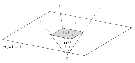
An effect respresents a measurement outcome. If a system in a state is measured with respect to a measurement , then is the probability that the measurement yields the outcome associated with .
Example C.3 (Quantum theory):
The probabilistic structure of measurements on a (finite-dimensional) quantum system can be formulated as an abstract state space. For a quantum system with an associated Hilbert space , consider the abstract state space , where is the real vector space of Hermitian operators on , is the cone of positive operators on and is the trace on . According to Definition C.2, this yields the states , which are precisely the density operators on . Analogously, are the subnormalized density operators. The effects are the functionals induced by POVM elements via the trace, . Accordingly, the measurements are the sets of functionals that are induced by POVMs, . This precisely reproduces the structure of measurement statistics in quantum theory. For further details, see [63].
By our definition, is the set of all linear functionals such that for all . The underlying assumption that every such linear functional represents a physical measurement outcome has been called the no-restriction hypothesis [40]. A priori, there seems to be no immediate physical reason for this assumption, and some authors have argued about how to weaken this assumption [64]. For our purposes here, it is not relevant whether the no-restriction hypothesis holds, and weakening the assumption complicates the definitions. Thus, we assume it for simplicity.
In Section C.2, we will define a decoherence quantity analogous to the quantum min-entropy . We will take our inspiration from expression (A.17) for the quantum min-entropy, which involves the fidelity as a measure of closeness of quantum states. Therefore, it is desirable to have a generalization of the fidelity to states in abstract state spaces. Such a generalization is easily found once it is noticed that the quantum fidelity of two states can be expressed as the Bhattacharyya coefficient (or classical fidelity) of the two probability distributions that the two states induce, minimized over all measurements. More precisely, the quantum fidelity satisfies [25]
| (C.5) |
where the minimization runs over all POVMs on the Hilbert space on which and are defined. The sum in (C.5) is precisely the Bhattacharyya coefficient of the probability distributions that the POVM induces on the states and . This motivates us to define the fidelity for abstract state spaces as follows.
Definition C.4:
Let be an abstract state space with normalized states and measurements . For states , we define the fidelity of and as
| (C.6) |
The quantity is the Bhattacharyya coefficient (or sometimes called the classical fidelity) of the probability distributions that the measurement induces on the states and .
The fidelity as defined in Definition C.4 precisely reduces to the quantum fidelity in the case where the abstract state space is a quantum state space. In addition to the fidelity, in Section C.3 we will also consider a generalization of the quantum trace distance in order to formulate a bound on . Somewhat analogously to the fidelity, the quantum trace distance is equal to the total variation distance (or classical trace distance) between the two probability distributions that the two states induce, maximized over all measurements [25]:
| (C.7) |
This motivates the following definition.
Definition C.5:
Let be an abstract state space with normalized states and measurements . For states , the trace distance between and is given by
| (C.8) |
The quantity is the total variation distance (or sometimes called the classical trace distance) between the probability distributions that the measurement induces on the states and .
Note that the fidelity and the trace distance take values between 0 and 1 for all states. For squares of the quantities , , and , we will write the square sign right after the letter, e.g. we will write instead of .
C.1.2 A tripartite framework for GPTs
In Section C.2, we will consider a tripartite situation for the decoherence analysis, analogous to appendix A. This requires us to model a tripartite scenario mathematically since such a structure is not induced by an abstract state space alone. We need to specify it as additional structure. Our goal here is to do this with the weakest possible assumptions, resulting in a very general validity of the bounds we derive.
Instead of assuming individual state spaces for every party, we only consider their overall combined state space, modelled by an abstract state space and all its induced structure as in Definitions C.1 and C.2. This has the advantage that we do not have to make assumptions about how individual state spaces combine to multipartite state spaces, keeping our assumptions weak. For our purposes, the only structure that we need to add to an abstract state space to make it suitable for the description of a tripartite scenario are the local transformations that each individual party can perform. The local measurements of the three parties are then induced by these local transformations.
We consider three parties, which we call Alice (), Bob () and Eve () as before. We begin our considerations by assuming that there are three sets , and , containing all the transformations that Alice, Bob and Eve can perform, respectively. By a transformation, we mean a linear map which maps states to subnormalized states, i.e. (or, equivalently, and for all ). We can consider the case where several transformations are applied because compositions of transformations are transformations again: If , are linear maps which map inside , then the same is true for the composition (we denote the composition of maps by a symbol).
We assume that the three parties act individually at spatially separated locations. Relativistic considerations lead to the consistency requirement that transformations performed by different parties must commute, e.g. if Alice performs a transformation and Bob performs a transformation , then the total transformation must satisfy .
For our purposes, we do not need to specify the sets , and any further; the only requirement is that transformations of distinct parties commute. The sets , and define the systems , and , i.e. we define the individual parties via the transformations that they can perform. This leads us to the following definition.
Definition C.6:
A tripartite scenario is a quadruplet
| (C.9) |
where is an abstract state space, and where
| (C.10) |
are such that for all with , it holds that for all and for all . We call the elements of , and the local transformations of , and , respectively.
It is absolutely natural to define tripartite scenarios via commuting transformations rather than via a tensor product structure. In quantum theory, the two approaches are equivalent in finite dimensions (we will talk about this below). In more general infinite-dimensional cases, where it is not known whether the two approaches are equivalent, things are usually formalized in a commutative way rather than via tensor products (see [65], for example). Knowing about the equivalence in finite dimensions, we will formulate some quantum examples in the tensor product structure below.
Example C.7 (A tripartite quantum scenario):
One can formulate a tripartite situation in quantum theory as a tripartite scenario. Based on Example C.3, consider the tripartite scenario
| (C.11) | ||||
| (C.12) | ||||
| (C.13) | ||||
| (C.14) | ||||
| (C.15) |
where CPM stands for completely positive map. Having tensor product form, the local transformations of different parties commute.
For our purposes, Definition C.6 is all the structure one needs to specify. The local measurements are induced by the local measurements. We formalize this via the noation of a local instrument [56]. To get an intuition for what an instrument is, consider a Stern-Gerlach experiment. A spin-1/2 particle enters a magnet and undergoes one of two transformations: It either gets deflected upwards or downwards. Which of the two transformations it undergoes is determined probabilistically. Then it hits a screen, which reveals which of the two transformations the particle has undergone. This way, a measurement has been performed in two stages: a probabilistic application of a transformation and a detection. The sum of the probabilities of detecting the particle at the top or the bottom of the screen is one. If the state of the particle is described by a state of an abstract state space, we may model this by a set of two transformations . Such a set is an instrument. The norm is the probability that the particle is deflected upwards, and likewise for . Thus, can be seen to play the role of the screen, detecting the particle. The requirement that the particle must undergo one of the two deflections reads . The transformation is the analogue of the transformation in quantum theory, where is the projector onto the spin-up state. Since is given by the trace in quantum theory, the probability for the upward-deflection to occur is given by , which is precisely the Born rule.
A local instrument is such a set of transformations where all the transformations are the local transformations of one party. This motivates the following definition.
Definition C.8 (Local instruments):
For a tripartite scenario with as defined in Definition C.2, we define the local instruments as the elements of
| (C.16) |
Example C.9 (Local instruments in a tripartite quantum scenario):
Considering the tripartite scenario of Example C.7, we get that the local instruments are given by
Remark C.10 (Local measurements):
The definition of local instruments gives us a notion of local measurements as well. Consider a tripartite scenario with its set of measurements . It is easily verified that for a local transformation , the map is an effect (as defined in Definition C.2). Likewise, for a local instrument , the set is a measurement. We interpret it as a measurement performed by Alice. We can also consider composite measurements where several parties locally perform measurements. For local instruments and , for example, the set is a measurement. We interpret it as a composite measurement where Alice and Bob each perform local measurements, described by and . The analogous holds for other parties and combinations thereof.
Example C.11 (Local measurements in a tripartite quantum scenario):
Based on Examples C.7 and C.9, we can say how local measurements look like in a tripartite quantum scenario. A local effect of Alice is of the form
| (C.17) |
for a trace non-increasing CPM on . However, for every such CPM, there is a POVM element on such that66 6 This can be seen from the Kraus representation of : for . (We omitted the other tensor factors for brevity.)
| (C.18) |
This recovers the Born rule. Analogously, a composite measurement where Alice and Bob each perform local measurements consists of local effects of the form
| (C.19) |
for POVM elements , on , . Thus, in our tripartite quantum example, local measurements reduce to POVM measurements of product form.
In Examples C.7, C.9 and C.11, instead of choosing a tensor factorization for and setting the local transformations to be acting non-trivially on one tensor factor, we could have chosen sets of transformations that merely commute, without a tensor product structure. The question of whether the resulting measurement statistics in that case would be different from the case with the tensor factor structure is known as Tsirelson’s problem [66, 67]. More precisely, the question is the following. Let be a Hilbert space, let be a density operator on , let , be POVMs on such that for all , . Tsirelson’s problem is: Does there necessarily exist Hilbert spaces , , a density operator on and POVMs on and on such that for all , ? In the case where is finite-dimensional, the answer is known to be affirmative. For infinite-dimensional Hilbert spaces, the answer is still unknown.
Thus, for finite-dimensional quantum systems, we can restrict ourselves to the case with the tensor product structure without loss of generality. For abstract state spaces, however, an analogous restriction might cause a loss of generality. The advantage of our weak definition of a tripartite scenario is that we do not need to know the answer to an equivalent of Tsirelson’s problem for generalized probabilistic theories. The downside is that it makes defining an equivalent of the min-entropy more difficult. We will deal with this issue in the next subsection.
Notation:
From now on, whenever we speak of a tripartite scenario , we implicitly assume that all its parts and induced structures are denoted as in Definitions C.1, C.2, C.6 and C.8 without restating it, i.e. instead of writing “Let be a tripartite scenario, let be its set of normalized states, …”, we will only write “Let be a tripartite scenario”.
C.2 A decoherence quantity for GPTs
C.2.1 Motivation of an expression that quantifies decoherence
We are now going to motivate an expression for the central quantitiy for our decoherence analysis for GPTs. We take our inspiration from expression (A.17) for the quantum min-entropy, which we repeat here for the reader’s convenience:
| (A.17 revisited) |
There are two issues that prevent us from directly translating expression (A.17) into our framework. The first issue is that in Section C.1.2, to keep our framework as general as possible, we have defined a tripartite scenario with an overall state space with tripartite states . We do not have notions of individual state spaces at hand. Thus, we do not have an analogue of a reduced state or of a transformation from one state space to another.
The second issue is that we do not know what the analogue of a maximally entangled state in our framework is. We resolve the first issue here in Section C.2.1, arriving at an expression for . In Section C.2.2, we will then define what a maximally entangled state is in our framework.
Expression (A.17), which involves the state and TPCPMs , can be transformed to an expression in which both the state and the TPCPMs are purified (see Figure 9). This expression will be our motivation for the expression for . The maximization over TPCPMs from to is replaced by a maximization over unitaries from to , where and are ancilla systems extending system and , respectively. This is precisely the purification (or Stinespring dilation) of a channel as in appendix A. Since systems and have the same dimension, we can identify their Hilbert spaces and regard the resulting Hilbert space as the Hilbert space of a system . This system involves all subsystems that the third party needs to control in order to bring itself as close as possible to maximal entanglement with Alice. Since is a transformation on system alone, we can translate it into our generalized framework.

The state is replaced by a purification . We choose the purifying system to be the channel’s output system, which gives us the overall picture of our decoherence analysis as shown in Figure 10.

The following gives a precise formulation of the purification of expression (A.17). It can be proved using purification and Stinespring dilation. Let , be finite-dimensional Hilbert spaces of dimensions , , respectively, let . Then, for any purification of , any Hilbert spaces , and of dimension , and , respectively, any maximally entangled state and any pure state , it holds that
| (C.20) |
where and where the first maximization ranges over unitaries
| (C.21) |
and the second maximization ranges over pure states .
Now we translate expression (C.20) into our generalized framework. We interpret the system as the system controlled by Eve, and therefore rename .
- •
Since we want to arrive at an expression that does not make unnecessary assumptions about the mathematical description of the physical situation, we avoid the factor present in (C.20). We look for a GPT analogue of , omitting . As a consequence, we will have in quantum theory (see Example C.14).
- •
We replace the maximization over all unitaries acting on system by a supremum77 7 We do not assume enough about to guarantee that the maximum is achieved, so we replace it by a supremum. over all local transformations . 88 8 One might raise the objection that in the quantum case, Example C.7, the unitaries only correspond to those elements of which bijectively map the space of density operators onto itself. It would be possible to include this restriction, but we decide not to do so, for two reason: We want to keep things simple, and we want to avoid the assumption that actions that the third party can perform can be purified as in the quantum case.
- •
We generalize the quantum fidelity to the fidelity in abstract state spaces as defined in Definition C.4.
- •
We replace the state by a state .
- •
If we look at the state , we see that it is a state of maximal entanglement between Alice and Eve in the sense that by performing measurements with elements of the form , they can get any statistics that two parties and would be able to get by performing local measurements on the maximally entangled state . We translate this into our framework by assuming that there is a set of “states with maximal correlation between Alice and Eve”. Instead of minimizing over states , we then minimize over the set .
We postpone the discussion of how such a set looks like. We will give a definition of such a set in Section C.2.2 below. For now, we write down an expression for our decoherence quantity that depends on the choice of such a set . According to what we have just discussed, the expression is
| (C.22) |
We interpret the decoherence to be high when this quantity is high and vice versa, which is the opposite of (see the end of appendix A). Before we can define , however, we need to specify what a maximally entangled state in a GPT is.
C.2.2 Definition of maximal correlation in GPTs
The expression (C.22) for our decoherence quantity contains a maximization over a set which we interpret to be the set of states with maximal correlation between Alice and Eve. We now define this set.
Definition C.12:
For a tripartite scenario , we define the set of states with maximal correlation between Alice and Eve by
| (C.23) |
Definition C.12 can be read as follows. The superscripts and of the elements of the instruments and stand for measurement outcomes, so or is the probability that Alice and Eve both get outcome or both get outcome , respectively, when they measure with respect to , , respectively. Thus, the sum of these probabilities is the probability that Alice’s and Eve’s measurement outcomes are perfectly correlated. This means that for a state , it holds that for every binary measurement of Alice, there is a binary measurement for Eve such that their measurement outcomes are perfectly correlated.
A closer look at some subtleties is advisable here, both to avoid confusion and to see the advantages of the weak assumptions that define our framework. With reference to Example C.11, one may point out that that the set
is empty. This may seem to make our definition of incompatible with quantum theory. Note, however, that the set
is not empty as long as . If, as in Section C.2.1, with , then this set contains all the states of the form with as in (C.20). The advantage of our weak definition of the local transformations is that it does not force to see as the analogue of the set of all CPMs of the form , but that it can be considered to be the analogue of all such CPMs which induce a functional of the form , where is a projector. Example C.11 can be modified accordingly (see Example C.14 below). This makes our definition of compatible with quantum theory.
With Definition C.12 at hand, we are finally ready to define the decoherence quantity.
Definition C.13:
Let be a tripartite scenario, let . We define the the decoherence quantity of by
| (C.24) |
Example C.14:
We consider a special case of a tripartite scenario in quantum theory. Consider
| (C.25) | ||||
| (C.26) | ||||
| (C.27) |
and analogously for and . In addition, we assume for simplicity that . In this case,
| (C.28) |
where is the set of maximally entangled states on analogous to (A.18). For a pure state , this gives us
| (C.29) | ||||
| (C.30) | ||||
| (C.31) |
Hence, .
C.3 Bounds on the decoherence quantity for GPTs
The goal of this subsection is to derive an upper bound on in terms of the CHSH winning probability of Alice and Bob. This is a practically relevant bound: On the premise that the channel behaves identically in multiple uses and does not build up correlations between different uses (such a channel is said to be iid, for independent and identically distributed), this winning probability can be estimated through repeated measurements on Alice’s and Bob’s side. What we show is that this estimate in turn gives a bound on . In this section, we formulate this bound as a minimization problem which we solve and interpret in Section C.4.
In the following, we derive a lower bound on . We make the convention that , where is a symbol for which we accept the inequality for every real number . This lower bound on then gives us an upper bound on . In a first step, we bound the fidelity-based quantity by a trace distance-based quantity. This has the advantage that the resulting optimization problems which give us the bounds can be solved using linear programming.
Proposition C.15:
Let be a tripartite scenario, let . Then
| (C.32) |
The following lemma is useful for the proof of Proposition C.15 below.
Lemma C.16:
For all , it holds that .
Proof.
We have that , so the claim is equivalent to
| (C.33) |
The functions and are differentiable on . Thus, by the fundamental theorem of calculus, it holds that for all ,
| (C.34) |
so for all , we have that
| (C.35) |
This proves the claim. ∎
Proof of Proposition C.15.
Since the right hand side of (C.32) is a finite real number, the inequality trivially holds if by the above convention. Thus, we assume in the following that . We have that
| (C.36) | ||||
| (C.37) |
For , it holds that (see Lemma C.16). Thus, since
| (C.38) |
we get that
| (C.39) | ||||
| (C.40) | ||||
| (C.41) |
For the Bhattacharyya coefficient and the total variation distance , it has been shown [68] that for any two probability distributions distributions, it holds that . Since this is true in particular for the two probability distributions that the measurement induces on the states and , we get that
| (C.42) | ||||
| (C.43) |
as claimed. ∎
The idea that the fidelity and the trace distance are related is not new. In quantum theory, the Fuchs-van de Graaf inequalities (FvdG) relate the two quantities [69]. Inequality (C.32) is not completely analogous to the FvdG inequalities: It makes use of the logarithm in (C.32), which allows to apply classical relations that lead to a stronger bound than with the application of the FvdG inequalities.
For the bounds that we are going to derive, the notion of a non-signalling distribution is central. Our bounds are essentially minimizations of functions over sets of non-signalling distributions and with certain additional properties.
Definition C.17:
A set of numbers , indexed by numbers which we call outcomes, and numbers which we call settings, is a non-signalling distribution if
| normalization: | (C.44) | |||||
| no-signalling: | (C.45) | |||||
| (C.46) | ||||||
| (C.47) | ||||||
Similarly, a set of numbers , indexed by outcomes and settings is a non-signalling distribution if
| normalization: | (C.48) | |||||
| no-signalling: | (C.49) | |||||
| (C.50) | ||||||
The interpretation of equations C.45, C.46 and C.47 is that it is impossible for each of the three parties to signal to the other two parties by influencing their measurement statistics with the choice of the measurement setting. These one-party no-signalling constraints imply all the multi-party no-signalling constraints, saying that no collection of parties can signal to the remaining parties [70], so we do not need to require these constraints separately.
Now we are going to formulate the bound on in terms of the CHSH winning probability of Alice and Bob. Assume that Alice, Bob and Eve are in a situation described by a tripartite scenario . Suppose that Alice and Bob have estimated that for the state that they are analyzing, their CHSH winning probability is at least for some . Formulated in our tripartite scenario language, this means that they have found out that for local instruments
| (C.51) | ||||
| (C.52) |
it holds that
| (C.53) |
In that case, what can Alice and Bob infer about ? We have seen in Proposition C.15 that this quantity is lower bounded by . Alice’s and Bob’s estimate on their CHSH winning probability can be translated into a bound on this quantity. This is shown by the following proposition.
Proposition C.18:
Let be a tripartite scenario, let be a state. If the CHSH winning probability of Alice and Bob is at least , i.e. if there are local instruments , , and as in (C.51) and (C.52) and a such that (C.53) is satisfied, then
| (C.54) |
where is the set of non-signalling distributions for Alice, Bob and Eve such that Alice and Bob have a CHSH winning probability of at least , i.e.
and where is the set of non-signalling distributions for Alice and Eve such that their measurement outcomes are perfectly correlated when they choose the same measurement setting, i.e.
| (C.55) |
Proposition C.18 reduces our problem of lower bounding the decoherence quantity for GPTs to an optimization over non-signalling distributions. This allows us to use linear programming techniques, which in similar ways have been used in [26] to answer questions about non-signalling distributions.
We need the following lemma for the proof of Proposition C.18 below.
Lemma C.19:
Let be a tripartite scenario, let . Then, for all local instruments , it holds that
| (C.56) |
Proof.
It is sufficient to show that for all , for all and for all ,
| (C.57) |
This is what we are going to show now. Let , let , let . Then
| (C.58) |
If instead of taking the supremum over , we only evaluate the expression for a particular element of , we get a lower bound on (C.58). We choose the element (c.f. Remark C.10)
| (C.59) |
Hence,
| (C.60) |
By the definition of a local instrument, . Thus,
| (C.61) | ||||
| (C.62) |
where in the last equality, we made use of the fact that transformations of different parties commute. ∎
Proof of Proposition C.18.
It is sufficient to show that for every , the claimed inequality holds without the minimization over , i.e.
| (C.63) |
By means of Lemma C.19, we know that for all and every ,
| (C.64) |
Let , let , be local instruments for Eve such that
| (C.65) | ||||
| (C.66) |
which exist according to the definition of (Definition C.12). It holds that for every ,
| (C.67) | ||||
| (C.68) |
where
| (C.69) | ||||
| (C.70) |
Hence,
| (C.71) |
forms a non-signalling distribution: For the normalization, note that for all , we have that
| (C.72) | ||||
| (C.73) |
For the no-signalling condition, note that for all , it holds that
| (C.74) | ||||
| (C.75) |
and that for all , it holds that
| (C.76) | ||||
| (C.77) |
where in the second equality, we made use of the fact that local transformations of different parties commute. Analogously, for every , is a non-signalling distribution. Moreover, satisfies
| (C.78) | ||||
| (C.79) | ||||
| (C.80) |
where the inequality is one of the assumptions of the proposition. Furthermore, satisfies
| (C.81) | ||||
| (C.82) |
(where we made use of (C.65) and (C.66)), which we may abbreviate as . Thus, for every , we have that and . Thus,
| (C.83) |
Since satisfies the no-signalling property, the right hand side of (C.83) is independent of , so the minimization only needs to be performed over and . Moreover, the infimum over the sets and is a minimum because it is the infimum of a continuous function over a convex polytope, which is always attained (see Section C.4 for more details). This completes the proof. ∎
Corollary C.20 (The bound):
Let be a tripartite scenario, let be a state. If the CHSH winning probability of Alice and Bob is at least (in the above sense), then
| (C.84) |
where
| (C.85) |
Proof.
This is a direct consequence of Propositions C.15 and C.18. ∎
C.4 Evaluation of the bound and results
C.4.1 Formulation of the bound as a linear program
In this subsection, we evaluate the bound (C.84). To this end, we rewrite (C.85) in terms of linear programs.
Linear Program:
The bound , which is a function , is given as follows. For all , the value is the solution of the linear program
|
This is a linear program in 97 variables:
We have already written out the constraints for these 97 variables as (in)equalities. The third and fourth line are already written as such in the program description, and for the first two lines, we refer to the following:
| constraint | (in)equalities |
|---|---|
| (C.44) to (C.47) and inequality in (C.18) | |
| (C.48) to (C.50) and equation in (C.55) |
The inequalities define a convex polytope over which the convex function is minimized, so the minimum is attained. It is straightforward to bring these inequalities into the standard form of linear programming. We solved the resulting linear program using standard linear programming routines in Mathematica and Octave.
C.4.2 Solution of the linear program and discussion of the results

We plot the result in Figure 11. The bound is non-trivial for values . This is a very satisfactory result as one cannot expect the bound to be non-trivial for : A CHSH winning probability of at least for Alice and Bob is always compatible with . To see this, note that the requirement for a state to yield a CHSH winning probability for Alice and Bob of at least is trivial: Alice and Bob can choose trivial measurements that always yields 1 as an outcome, independently of the state. More precisely, in our tripartite scenario language, we can express this as follows. Certainly, there are tripartite scenarios in which the identity map and the zero map are in , and .99 9 Every tripartite scenario can be turned into such by adding and to the sets of local transformations. In fact, it would be physical to assume that each set of local transformations contains and . For such tripartite scenarios, the condition (c.f. (C.51) to (C.53) in Section C.3)
is always satisfied because for all ,
This means that the requirement that the CHSH winning probability for Alice and Bob is at least does not exclude the case . In that case, .
Appendix D A test for gravitational decoherence
D.1 An optomechanical setting and its model for gravitational decoherence
The objective here is to create two entangled photonic qubits in which one photon is prepared in an opto-mechanical system that is itself subject to gravitational decoherence — if there is any — and the other photon is prepared in an identical cavity except the mirrors are fixed and cannot move. This model is a modification of the model first proposed by Bouwmeester [5] in which an itinerant single photon pulse is injected into a cavity rather than created intra-cavity as here. Our modification avoids the problem that the time over which the photons interact with the mechanical element is stochastic and determined by the random times at which the photons enter and exit the cavity through an end mirror. In the new scheme, the cavities are assumed to have almost perfect mirrors — very narrow line width (see for example[35]).
The intracavity single photon Raman source is described in Nisbet-Jones, et al. [34]. In this scheme (see Fig. 12) a control pulse can quickly and efficiently prepare a cavity mode in a single photon state by driving a Raman transition between two hyperfine levels we label as . In our scheme there are two optical cavities otherwise identical except in one of the cavities a mechanical element can respond to the radiation pressure force of light.
We will assume that we can prepare the atomic sources in an arbitrary entangled state , for example, using the trapped ion schemes of Monroe [71]. In addition we will assume that we can make arbitrary rotations in the subspace of each source and also make fast efficient single shot readout of the state of each source, for example using fluorescence shelving. This means we can readout the atomic qubit in each cavity in any basis.
The write laser implements the Hamiltonian . This is a rotation in the state space . We can thus prepare arbitrary states of the form , where is determined by the pulse area. We will refer to the case of as a -pulse. Note that if the source is in the excited state and the cavity is in the vacuum, no photon is excited.
Starting with the cavities in the vacuum state the protocol proceeds as follows:
- 1.
prepare the source atoms in the state .
- 2.
apply the write laser with a -pulse
- 3.
free evolution of the OM systems for a time
- 4.
apply the write laser with a -pulse
- 5.
readout the atomic state in each cavity.
At the end of Step 2, the state of the sources and the cavities is where with each factor being a photon number eigenstate.
D.1.1 Gravitational decoherence.
We will use Diosi’s theory of gravitational decoherence[1]. This is equivalent to the decoherence model introduced in Kafri et al. [9]. One mirror of the opto-mechanical cavity is free to move in a harmonic potential with frequency . The master equation for a massive particle moving in a harmonic potential, including gravitational decoherence is
| (D.1) |
where
| (D.2) |
with the usual canonical position and momentum operators. The gravitational decoherence rate is given by
| (D.3) |
with the Newton gravitational constant and the density of the mechanical element. As one might expect is quite small, of the order of s-1 for suspended mirrors ( as in LIGO) with .
Form a phenomenological perspective the effect of gravitational decoherence is analogous to a Browning heating effect. To see this we note that the average vibrational quantum number increases diffusively
| (D.4) |
Indeed, one could simulate this effect by adding a stochastic driving force to the mechanical element via the stochastic Hamiltonian
| (D.5) |
where satisfies an Ito stochastic differential equation,
| (D.6) |
where is the Weiner increment. Averaging over all histories of the stochastic driving force gives the final term in Eq. D.1.
In the absence of mechanical dissipation, there is no steady state. In reality the mechanical quality factor, , is finite leading to a steady state with mean phonon number given by
| (D.7) |
This of course assumes that there is no additional mechanical heating (regular thermodynamic kind): hardly a realistic assumption. This adds a large (comparatively) additional term to so that we find (for ),
| (D.8) |
Given the incredibly large quality factor of , one would need to cool the mechanical element to nano-Kelvin for the thermodynamical heating to be of the order of the gravitational heating.
D.1.2 Optomechanical probe of gravitational decoherence.
The optomechanical Hamiltonian in cavity-one is
| (D.9) |
is the single photon optomechanical coupling rate. Typically s-1 for the sorts of cavities we are considering here. This is about the same order of magnitude as . In new field OM cavity technologies, can be as high as s-1 however in such cases the mechanical frequency is also typically much higher tens of MHz. The interaction time is which is short compared to the cavity decay time (which we neglect). We will assume that the mechanics starts in a thermal state, the steady state of the system subject to gravitational decoherence, heating and dissipation. This is given by
| (D.10) |
where is the steady state mean phonon number given in Eq. D.7.
It is simplest to work in an interaction picture defined by the mechanical free dynamics,
| (D.11) |
The corresponding unitary evolution operator is
| (D.12) |
where
| (D.13) |
The initial state for the OM interaction is the state at the end of Step 2
| (D.14) |
where is the state of the mechanical element at the start of the protocol, a thermal state. We can ignore the state of the atomic sources at this stage as they do not participate in the OM interaction.
The state of the optomechanical system after an interaction time is given by
| (D.15) |
The reduced state of the cavity fields is given by tracing out the mechanical degree of freedom,
| (D.16) |
where
| (D.17) |
where
| (D.18) | |||||
| (D.19) |
with (as above)
| (D.20) |
and
| (D.21) |
Continuing with the protocol from Step 4, now results in the state of the atom-field system
| (D.22) |
where
| (D.23) |
The suppression of coherence due to the thermal state of the mechanics has been transferred to a reduction of entanglement in the atomic sources. A readout of the atomic sources will reveal this through either state tomography or via a reduction in a CHSH correlation for a Bell-type experiment.
The function is a periodic function of time. At each period of the motion it returns to its initial value of zero and the cavity field state would return to the fully entangled state it was in after Step 2. If we chose then the protocol will return the atomic system to the same entangled state in which it began. This is because we have ignored the heating of the mechanics over the period so the only way decoherence enters is through the initial thermal excitation of the mechanics. In effect the protocol is a thermometer. We thus see that for maximum effect we need to ensure . On the other hand, gravitational heating requires a small value of and typically such OM systems have . Perhaps technical advances will enable OM systems with long mechanical periods and large single photon coupling. Of course this will also require sub hertz cavity line widths. In the (exceptionally) optimistic case we can take nK, s-1, s-1 so that .
D.2 An experimental test of the model
In Section D.1 above, an optomechanical setting has been described. Making some assumptions about how gravitational decoherence influences the optomechanical system, a model has been given that describes how the state of the optomechanical system changes over time. In this section, we consider this model for the state of the optomechanical system as given and analyze it using our decoherence test formalism. We calculate the amount of decoherence that would be introduced to the optomechanical system if the model was correct. We compare this to the amount of decoherence that one would observe if there was no such gravitational decoherence, determining the difference between the two predictions. We devise an experiment that aims at estimating the actual amount of decoherence at a point in time when this difference is maximal. This turns the optomechanical experiment into a test that allows to falsify the above model for gravitational decoherence if it was wrong. This shows that the decoherence testing formalsim presented in this work can be applied in situations where the physical process is unknown. It allows to subject proposed models of the process to a consistency check.
We first present the predicted values of of the optomechanical system for the two cases where gravitational decoherence is present or absent, respectively, for some example parameters of the experiment. We then calculate the CHSH value that one would have to measure in order to falsify the model for gravitational decoherence.
The main quantity of interest in our analysis is the decoherence quantity for the state desribed in equation (D.16). This can be calculated using Lemma B.9. It turns out to be
| (D.24) | ||||
| (D.25) |
If the above model is correct and gravitational decoherence occurs, both the gravitational interaction and the mechanical heating contribute to the average vibrational quantum number, i.e. we have
| (D.26) | ||||
| (D.27) |
and thus
| (D.28) |
If gravitational decoherence is absent, then only the mechanical heating contributes to the average vibrational quantum number, i.e. we have
| (D.29) | ||||
| (D.30) |
and thus
| (D.31) |
Figure 13 shows how the decoherence quantity in equation (D.28) as a function of time varies for different materials of the mechanical element and different temperatures, compared to the case where there is no gravitational decoherence as in equation (D.31).

In order to rule out the model for gravitational decoherence, one needs to measure a CHSH value which is incompatible with the value of given in (D.28). The minimal value of that needs to be measured for this falsification can be calculated using Theorem B.1: Using MATLAB, we numerically evaluated the quantum bound on , which is given as a point-wise maximization problem in Theorem B.1. We inverted the resulting set of data points and interpolated a function from the resulting data using Mathematica. The resulting function takes a value of as its input and outputs the minimal that needs to be exceeded in a measurement in order to rule out the given value of . Thus, applying this function to the curves of the values of the gravitational decoherence model in Figure 13 yields the curves for . The results are plotted in Figure 14 for the same materials and temperatures as above.
In order to determine whether it is promising to measure a value of that lies above , we need to determine the value of which is predicted in the case where gravitational decoherence is absent, i.e. where we only have mechanical heating. We can do that exactly: Equation (D.16) gives us an expression for the state, which we consider for the value of given in the case of mechanical heating only, . Then we calculate the value of for the case where the measurements are taken to be the standard CHSH measurements
where , are the Pauli - and -operator, respectively. The resulting curves are shown in Figure 14 as solid curves. It turns out that for the relevant time interval (where is larger than either of the ), the curve of for the standard CHSH measurements is almost identical to the curve one would get for the optimal measurements for each time . The latter can be calculated using a formula presented in [24]. This is an experimentally desirable fact: Using a fixed measurement independent of the measurement time is almost optimal.
The most promising measurement time for a falsification of the gravitational decoherence model is given by the time when (that one may hope to actually measure) is high but (which one needs to exceed) is low. Thus, the optimal measurement time can be calculated as the time that maximizes the gap function
| (D.32) |
This gap function is depends on the density of the mechanical element and its temperature . One can see that temperatures that look promising for a falsification measurement when looking at the values in Figure 13 turn out to be too warm when looking at the experimentally relevant analysis of the values in Figure 14. As an example, we have calculated the optimal measurement times for for the densities of aluminum and rhenium. They are visualized in Figure 15. If there is no gravitational decoherence, one needs to measure values of that are close (aluminum) or close (rhenium) to the value that one can maximally measure using the standard CHSH measurements, in order to exclude gravitational decoherence.