How to perform QCD analysis of DIS in Analytic Perturbation Theory
Abstract
We apply (Fractional) Analytic Perturbation Theory (FAPT) to the QCD analysis of the nonsinglet nucleon structure function in deep inelastic scattering up to the next leading order and compare the results with ones obtained within the standard perturbation QCD. Based on a popular parameterization of the corresponding parton distribution we perform the analysis within the Jacobi Polynomial formalism and under the control of the numerical inverse Mellin transform. To reveal the main features of the FAPT two-loop approach, we consider a wide range of momentum transfer from high to low where the approach still works.
pacs
12.38.Cy, 12.38.Aw, 12.38.LgI Introduction
QCD analysis of deep-inelastic scattering (DIS) data provides one with new knowledge of hadron physics and serves as a test of reliability of our theoretical understanding of the hard scattering of leptons and hadrons. At large momentum transfer GeV2 we have the reliable description of DIS that is based on the twist expansion and “factorization” theorems. At small (moderate) transfer (a few) GeV2 this QCD description faces two main problems: (i) the high twist corrections to the leading twist contribution become important but remains poorly known; (ii) perturbative QCD (pQCD) becomes unreliable due to the fact that the QCD running coupling grows and “feels” infra-red Landau singularity appearing at the scale of a few tenth of GeV. We discuss in this paper a solution of the last problem by applying to DIS analysis a nonpower perturbative theory whose couplings have no singularity at and whose corresponding series possess a better convergence at low .
A widely used approach to resolve the aforementioned problem is to apply the Analytic Perturbation Theory (APT) developed by Shirkov, Solovtsov et al. [1, 2, 3, 4, 5]. There, the running QCD coupling of pQCD is transformed into an analytic (holomorphic) function of , , APT coupling. This was achieved by keeping in the dispersion relation the spectral density unchanged on the entire negative axis in the complex -plane (i.e., for ), and setting it equal to zero along the unphysical cut . In the framework of APT the images of integer powers of the originals , following the same dispersion relations were also constructed. At low the couplings change slowly with in contrast with the original behaviour while at high . Later, the correspondence was extended to noninteger powers/indices in [6, 7, 8, 9, 10] and was called Fractional APT (FAPT), which provides the basis for application to DIS. In this respect let us mention a recent papers [11] where the processing of the DIS data has been performed in FAPT in the one-loop approximation and the reasonable results for hadron characteristics has been obtained.
Various analytic QCD models can be constructed, and have been proposed in the literature, among them in Refs. [13, 14, 15, 16, 17, 18, 19]. These models fulfill certain additional constraints at low and/or at high . For further literature on various analytic QCD models, we refer to review articles [20, 21, 10]. Some newer constructions of analytic models in QCD of include those based on specific classes of functions with nonperturbative contributions [22] or without such contributions [23, 24, 25] and those based on modifications of the the spectral density at low (positive) where is parameterized in a specific manner by adding two positive delta functions to , cf. [26].
The possibility to extend the DIS analysis formally in the whole range together with the effect of slowing-down of the FAPT evolution of the parton distribution functions (PDF) in the low region are attractive phenomenological features of FAPT. A number of works deal with this task in a naive form [27], where the authors show that at very low and Bjorken variable APT agrees with experimental data. Besides, the applicability of the APT approach was analyzed in the Bjorken polarized sum rule [28] confirming that the range of validity of APT is down to MeV, as compared to experimental data. The common feature of these works was taking into consideration some nonperturbative effects against the background of APT, i.e., higher twists in [27, 28, 29] or an effective constant gluon mass in [30].
The basis for applying FAPT to low energies in this approach is the factorization theorem that allows one to shift the frontier between the perturbative and nonperturbative effects via the variation of the factorization scale. Therefore, we shift the range where perturbation series is applicable in FAPT, as it was demonstrated in [28] (see reviews of this issue in [10], where this phenomenon was also discussed for pion form factors).
Our goal here is to elaborate a general scheme of DIS data processing in the framework of FAPT taking as a pattern the DIS analysis at NLO. In this respect the discussion here can be considered as an extension of the partonic results of the article [11] on the higher-loop level. We shall focus on the specifics of the Dokshitzer-Gribov-Lipatov-Altarelli-Parisi (DGLAP) evolution of the PDF in FAPT. We involve into consideration the coefficient function of the process and compare the final result with a similar one in pQCD. An important problem of higher twist contribution remains untouched here, but higher twist effects can be taken as an unknown function , i.e. [11], or as a constant [28] , or as an effective sum of all twists contributions in [29]. We stress that HT effects are only indirectly affected by the analytization procedure. The behavior of HT will be given by the fit of experimental data together with the corresponding parton distribution functions [11, 27, 28]. Besides, in [28] the authors included more terms in the HT expansion and demonstrated that they are essentially smaller and quickly decreasing. Because of this (theoretically) unknown behavior we avoid this problem since we pretend to provide perturbation tools how to deal with FAPT, while the pure phenomenological analysis is transferred to future investigations.
Let us recall that the DIS analysis can be performed in a few different ways: one of them is provided by the Mellin moments defined via inelastic structure functions (SFs) ,
| (1) |
The second approach is based on the direct application of the DGLAP integro-differential evolution equations [31] to PDF , while the observable SF is the Mellin convolution of the coefficient function and PDF, . The third approach makes use of the Jacobi Polynomial expansion method [32]. Just this method will be used in this work.
The paper is organized as follows: in Sec. II, we present a theoretical background where we describe the Jacobi Polynomial (JP) method and how to calculate free parameters in order to obtain the nonsinglet structure function. In Sec. III, we briefly describe the FAPT approach and derive the DGLAP evolution for the moments in FAPT. We present in Sec. IV the free parameters obtained in the analysis of the so called MSTW parameterization, see [33] for details, and the nonsinglet SFs at LO. Section IV contains the results of the analysis of numerical realization of the FAPT evolution and the comparison with the results of analogous calculations in pQCD. Finally, in Sec. V we summarize our conclusions. Important technical details including new findings are collected in four appendices.
II Jacobi Polynomial expansion for DIS analysis
We shall focus here on nonsinglet (NS) structure functions, , with their corresponding Mellin moments (via Eq. (1)) to avoid technical complications of the coupled system solution in the singlet case. The PDFs are universal process-independent densities explaining how the whole hadron momentum is partitioned in , i.e., the momentum carried by the struck parton (see, for instance [34]). The -dependence of PDF is formed at a hadron scale of an order of by nonperturbative forces, while its dependence on factorization/renormalization scale can be obtained within perturbation theory.
A brief description of the evolution of the Mellin moments in pQCD, up to NLO, is outlined in Appendix B as well as the theoretical background with our notation and conventions. We consider the scale as a reference scale for the solution of the evolution equation (33a) where the PDFs are regarded as functions of and the parameters are fixed by comparison with DIS data. In particular, we use here the data-based MSTW PDFs (see [33], where ). Namely,
| (2) | |||||
| (3) |
where the values of (), and can be found in [33]. We use only the valence quark PDFs because the NS PDF can be expressed as (see Appendix B for details). The NS SF is represented as the Mellin convolution of coefficient function of the process and the corresponding PDF . The can be expanded in the Jacobi Polynomials , which was developed in Refs. [32], in truncating the expansion at , where the method converges (see, for review [35]):
| (4) |
Here are the Mellin moments of nonsinglet SF calculated explicitly in Eq. (33a); is the weight function and the parameters will be obtained by fitting to the data. The Jacobi Polynomials are defined as an expansion series by means of
| (5) |
They satisfy the orthogonality relation
| (6) |
Another way to obtain SF is to take the inverse Mellin transform under the moments (i.e., the inverse of Eq. (1)). Choosing a convenient path of integration one obtains for
| (7) |
here we take the path along a vertical line . We perform the “exact” numerical Inverse Mellin Transform, further comparing the results with the Jacobi Polynomial method, only at the one-loop level due to technical limitations. In this way, we estimate the accuracy of the applied polynomial method, the results of this numerical verification are outlined in Appendix C.
Let us finally mention that one can take SF instead of the NS to consider, e.g. , the neutrino DIS results of the CCFR collaboration, like it was started in [11]. This replacement will lead to only minor changes of technical details in the procedure elaborated below.
III Fractional Analytic Perturbation Theory and DIS
It is known that the perturbative QCD coupling suffers from unphysical (Landau) singularities at . This prevents the application of perturbative QCD in the low-momentum spacelike regime and, in part, impedes the investigation of high twists in DIS. Our goal here is not to discuss the motivation and complete construction of FAPT, which couplings are free of the aforementioned problems, but present to reader illustrations of the properties of this nonpower perturbation theory that are important for further DIS analysis.
III.1 Elements of FAPT
Application of the Cauchy theorem to the running coupling , established in [1, 2, 3, 4, 5] and developed in [6, 7, 8, 9, 10], gives us the following dispersion relation (or Källén-Lehmann spectral representation) for the images in the spacelike domain
| (8) |
(where ) that has no unphysical (Landau) singularities. For the timelike regime analogous coupling reads
| (9) |
Here, is the FAPT image of the QCD coupling in the Euclidean (spacelike) domain with and the label denotes running in the -loop approximation, whereas in the Minkowski (timelike) domain, we used in (9) . It is convenient to use the following representation for the spectral densities :
| (10) | |||
From the definition (8) and Eq.(10) it follow that there is no standard algebra for the images , i.e. that justifies the name nonpower perturbative theory.
In the one-loop approximation, the has the simplest form, i.e.,
| (11) |
Substituting Eq.(11) in Eq.(10) for and then the result in Eq.(8), one reproduces at the well-known expression for maximum value of , [1],
| (12) |
At the two-loop level, they have a more complicated form. To be precise, one gets
| (13) |
and
| (14) |
with being the appropriate branch of the Lambert function, , , where are the QCD -function coefficients and is the number of active quarks, see the expressions in Appendix A. For our purpose we use here only the two-loop couplings like . Extensions up to four-loops can be found in [36].
Now we implement this formalism with the help of numerical calculation with the main module Mathematica package FAPT.m of [36] (confirmed by a recent program in [37]). According to this and using the corresponding notation from [36] in the RHS of Eqs.(15-17), we have
| (15) | |||||
| (16) |
For the coupling in pQCD we obtain
| (17) |
The correspondence between the pQCD expansion and FAPT one is based on the linearity of the transforms in Eqs.(8) and (9), see [5]. This can be illustrated for the simple case of a single scale quantity , calculated within minimal subtraction renormalization schemes and taken at the renormalization scale . The expansions for and for its image are written as
| (18) |
at the same coefficients that are numbers at .
III.2 FAPT for DGLAP evolution in NLO approximation
We start with the well-known solution of DGLAP equation for the nonsinglet PDF in NLO approximation. This solution is combined with the corresponding coefficient function – the parton cross-section taken at the parton momentum . This is presented in Appendix B in the form of Eq.(33a) for the moments of the NS SF .
Rewriting Eq. (33a) in the approximate form, i.e., neglecting the terms in the two-loop evolution factor, one arrives at the commonly used relation
| (19) |
The use of FAPT will change in this scheme the sense of expansion parameters in accordance with (18). An analogous evolution relation for the analytic images of the moments , , can be obtained from Eq.(19) by replacing the powers with the FAPT couplings (with being here an index rather than a power) [8] and reads
| (20) |
The implementation of the proposed calculation in the form of (15,17) is quite direct. The FAPT evolution relation (20) for the moments is the main result of the Section. Further, we shall use code (15) from [36] to obtain numerically.
The last approximation was taken up to since the contribution of the next term in the FAPT expansion in Eq.(20) is negligible in comparison with the previous one (as we demonstrate in Appendix D). This analytic version of the moment evolution does not face any problems at low energies due to the boundedness of couplings and rapid convergence of the FAPT series.
In the absence of a fit of experimental data for the FAPT model we propose a relation for the initial moments at :
| (21) | |||||
where the moment of PDF (see Eq.(30)) in pQCD stands in the LHS, while the moment for PDF in FAPT stands in the RHS of the second equation. In other words, we take the same initial PDF as in pQCD from the MSTW data for these both cases (in [11] the parameters were taken the same since the difference between them was negligible). We can use either the Jacobi Polynomial expansion or directly the inverse Mellin transform ( Appendix C).
IV Results of numerical analysis
The accuracy of the SF approximation by a finite number of Jacobi Polynomials (truncated at ) depends on the choice of the weight-function parameters. Therefore, we test the nonsinglet SF, given by the MSTW data, by searching for the minimum of ():
| (22) |
where we have used Eqs. (1) and (33a) at . Thus, we have and from Eq. (4) . Then, we determine the values of and that provide the best fit to the data for different values of . At the one loop level we find: , , and for , whereas for two loops we get (for even PDFs only): , , and for . To evolve nonsinglet moments, we need to fix the values of the QCD scale in the leading and next-to-leading order, taken in [33] from the comparison with data, where and . In the case of FAPT, the scales must be taken into account very carefully. The authors of [11] fixed the value directly from the comparison with the data in the leading order (where ) and obtained that corresponds to . We can see that the perturbative and the analytic values of are close to each other at least inside the margin of errors. For this reason, we will take for simplicity (recalling that an appropriate value should be taken from the analysis of the experimental data but this goes beyond the scope of this work). The couplings in pQCD and in FAPT were calculated with the Mathematica package developed by Bakulev and Khandramai in [36] where the heavy flavour thresholds were taken into account.
Taking into account the above estimates of the initial parameters, we substitute Eqs. (19) and (20) into Eq. (4), and obtain the evolution of SFs up to NLO in pQCD or FAPT, respectively. We show the final results of the evolution in Figs. 1, 2 using for DIS the character interval .
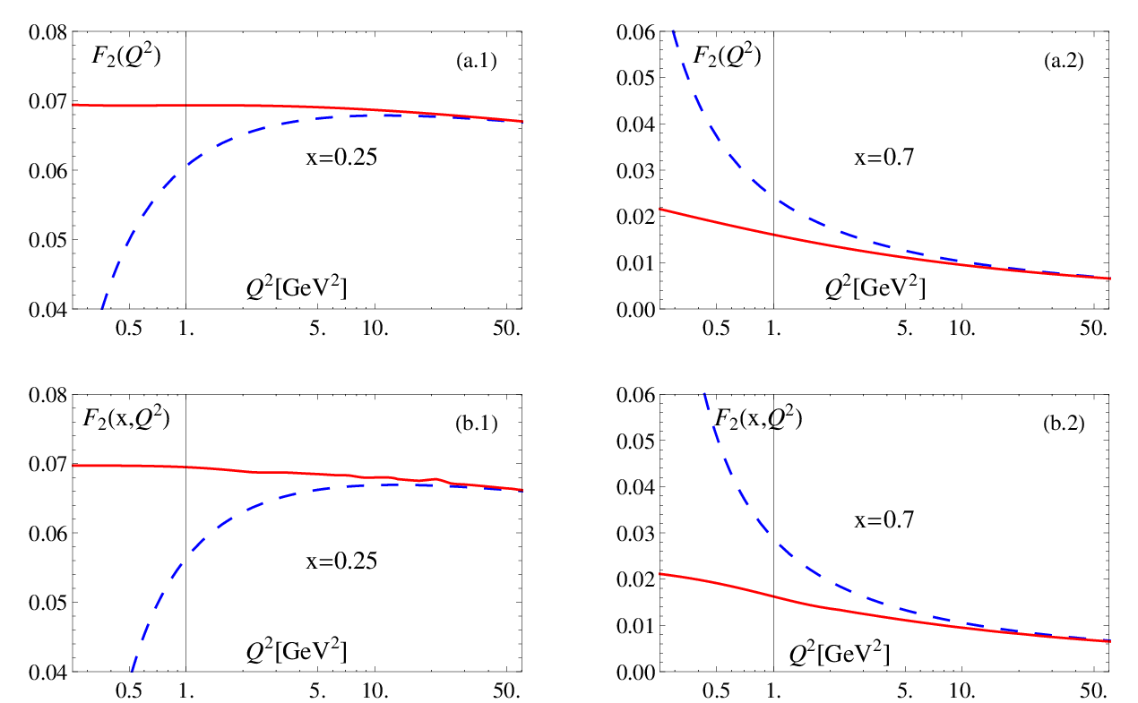
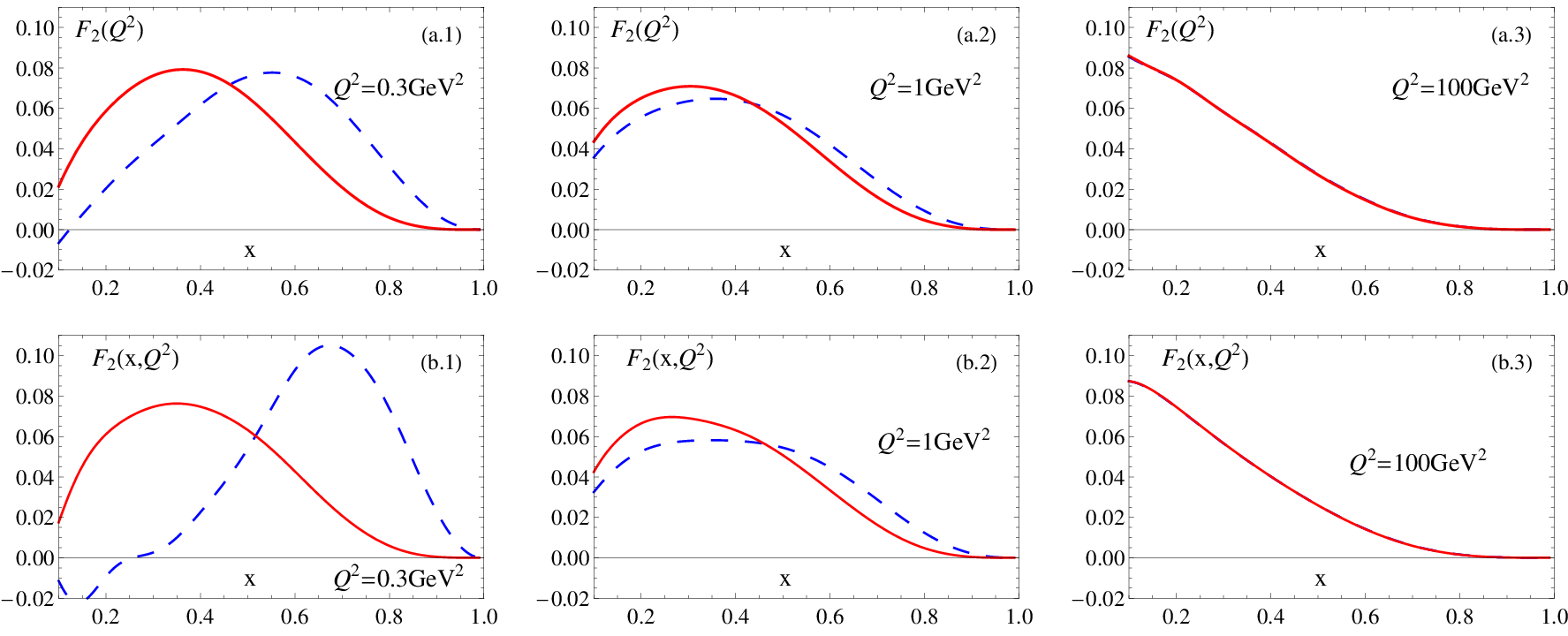
In Fig. 1 we fix at two different values: in (a.1), (b.1), and in (a.2), (b.2), where (a) and (b) represent the LO and NLO results, respectively. In Fig. 2, we fix at three different values: in (a.1), (b.1), with the initial point in (a.2), (b.2), and in (a.3), (b.3), where again (a) and (b) represent the LO and NLO, respectively.
V Summary
The main goal of this work is to propose a new theoretical tool for the DIS analysis, based on Fractional Analytic Perturbation Theory, to the DIS community. This approach allows one to analyze formally the leading-twist structure function in the whole range. This conclusion is explicitly shown in Figs. 1 and 2. The scheme of the approach is formulated in Sec. III and applied for data processing in Sec. IV. Our consideration is restricted to the leading twist. The higher twist contributions (HT) can be taken into account by a fit of experimental data together with PDFs. Moreover, the role of the stability of APT for this fit was pointed out in [11, 27, 28, 29] (and in Introduction here). Our investigation reveals the following main features of applying FAPT:
- •
Structure function at fixed changes very slowly in the entire range of .
- •
At high evolution () the pQCD and FAPT distributions become practically equal.
- •
The evolution in FAPT is more gradual (i.e., it evolves slower) and smoother than in pQCD.
- •
In this work, we have analyzed only the nonsinglet part, the consideration of the singlet part can be performed along the same line but requires more complicated formulas and cumbersome numerical calculations. This is the task for forthcoming investigation. Other important issues to complete this FAPT approach as the reliable tool for DIS is to add the target mass corrections (TMC) and the aforementioned HT contributions in our scheme of calculation. These improvements will help one to clarify in future the behavior at very low energies () in more detail. It would be important to emphasize, that the FAPT approach admits investigation of the HT contributions in the most sensitive regime of moderate/small due to the high stability of the radiative corrections.
Acknowledgements.
This investigation was started by the late A. P. Bakulev to whom we dedicate this work. We are grateful to G. Cvetič for useful comments and to N. G. Stefanis for careful reading of the paper and many valuable critical remarks. We thank A. V. Sidorov and O. P. Solovtsova for the useful remarks. This work was supported by the scientific program of the the Russian Foundation for Basic Research Grant No. 14-01-00647, BelRFFR–JINR grant F14D-007 (S.V.M), and by CONICYT Fellowship “Becas Chile” Grant No.74150052 (C.A).Appendix A Explicit expressions for NLO -functions, anomalous dimensions and coefficient functions of DIS (nonsinglet case)
The renormalization group equation for at the expansion of the -function up to the NLO approximation is given by
| (23) |
where the first two beta coefficients are
| (24) |
The anomalous dimensions of composite operators in LO, , NLO and the coefficient function are expressed by means of transcendental sums , see, e.g., [38],
| (25a) | |||||
| (25b) | |||||
| (25c) | |||||
On the other hand, the series can be expressed via the generalized Riemann functions, see [39], that are analytic functions in both variables :
| (26a) | |||||
| (26b) | |||||
| (26c) | |||||
| (26d) | |||||
For the and series we use the notation given in [40, 41]. Performing the analytic continuation from even , , and from odd , ( see for details [41]) one obtains
| (27a) | |||
| (27b) | |||
where is the Lerch transcendent function [39]. The expressions on the r.h.s. of Eqs.(27) are now analytic functions in both variables – this is a new result.
Appendix B QCD evolution of moments up to NLO
The PDFs are the nonsinglet and singlet parton distribution functions,
| (28) | |||||
| (29) |
whereas is the distribution of valence quarks and is the sea quark distribution. More generally, the NS PDF is a combination of the forms and but for our consideration we focus on the nucleon scattering provided by combination (B1). The moments representation for PDFs is defined as
| (30) | |||||
| (31) |
The moments for the structure function follow from the Mellin convolution ,
| (32a) | |||||
| (32b) | |||||
Here is the nonsinglet coefficient function of the process that can be presented as the perturbation series ; in Appendix A is the moment of the . The QCD evolution of the moments up to NLO of is given by (see Ref [38])
| (33a) | |||
| where | |||
| (33b) | |||
| and: | |||
| (33c) | |||
The coefficients of anomalous dimension in LO and NLO and the coefficient function in NLO are given in Eqs.(25a), Appendix A. In the case of the nucleon structure function , one needs to take into account only even values of in the NLO anomalous dimension.
Appendix C Accuracy of the Jacobi Polynomial method
The accuracy of the evaluation of the structure functions depends on the method we use; therefore, it is indispensable to verify it in our approach. The Jacobi Polynomial method promises us a good enough accuracy for the evolution, as was shown in previous works (see [32]).
This method is applied directly to the terms of the Bjorken variable , but it affects the -dependence indirectly. Therefore, it is necessary to confirm the -range applicability of the JP method. To this end, we compare the results of the JP approach with the “exact” numerical calculations of inverse Mellin moments following Eq. (7) but only in the one-loop approximation due to technical limitations.
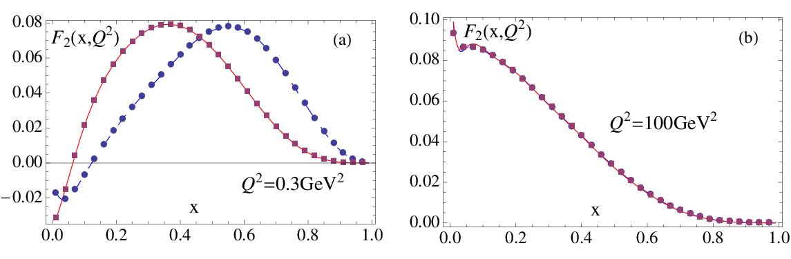
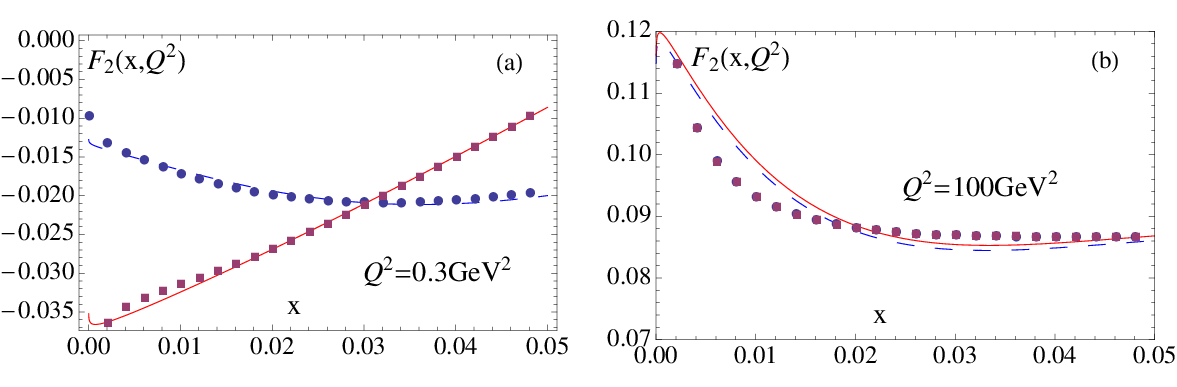
The comparison of these two results in Fig. 3 demonstrates a very good accuracy. So, in order to clarify it, we perform a zoom in , going to a lower -region (). We see in Fig. 4 that the JP method gradually loses precision starting at . Also, we can see that in this range, the difference between these two methods reaches %.
Appendix D Accuracy of the rational approximation
Here we investigate the accuracy of the rational approximation for the two-loop evolution factor
| (34) |
in Eq.(19) for pQCD, and Eq.(20) for FAPT, respectively. The expansion of the factor in power series up to NLO leads
| (35a) | |||||
| (35b) | |||||
where and represent the approximation up to and , respectively. The corresponding “FAPT form” of (35) is given by
| (36a) | |||||
| (36b) | |||||
Combing the approximations in Eqs. (35, 36) in quantity we obtain the accuracy better than for any (since JP expansion contains only 13 terms for good approximation), in both cases of pQCD and FAPT for two different ranges of energy, i.e., low and high . The results collected in Table 1
| 2 | 4 | 6 | 8 | 10 | 12 | |
|---|---|---|---|---|---|---|
| 0.74/ | / | / | / | / | ||
| / | 0.65 | 0.45 | 0.25 | 0.06 | 0.12 | 0.3 |
| 0.03 / | / | / | / | / | ||
| / | 0.18 | 0.13 | 0.07 | 0.02 | 0.04 | 0.09 |
demonstrate that for both ranges of energy FAPT has a better convergence than pQCD; even more, the accuracy is improved for FAPT at low (really, pQCD must be worse but we have a low starting point ). The strong hierarchy of FAPT couplings, , remains valid even at very low , cf. [10].
References
- [1] D. V. Shirkov and I. L. Solovtsov, [hep-ph/9604363]; Phys. Rev. Lett. 79, 1209 (1997) [hep-ph/9704333].
- [2] K. A. Milton, I. L. Solovtsov Phys. Rev. D 55, 5295 (1997) [hep-ph/9611438].
- [3] K. A. Milton, I. L. Solovtsov and O. P. Solovtsova, Phys. Lett. B 415, 104 (1997) [arXiv:hep-ph/9706409].
- [4] K. A. Milton, O. P. Solovtsova Phys. Rev. D 57, 5402 (1998) [hep-ph/9710316].
- [5] D. V. Shirkov, Theor. Math. Phys. 127, 409 (2001) [hep-ph/0012283]; 119, 438 (1999).
- [6] A. I. Karanikas and N. G. Stefanis, Phys. Lett. B 504, 225 (2001) [Erratum-ibid. B 636, 330 (2006)] [hep-ph/0101031].
- [7] A. P. Bakulev, S. V. Mikhailov and N. G. Stefanis, Phys. Rev. D 72, 074014 (2005) [Erratum-ibid. D 72, 119908 (2005)] [hep-ph/0506311].
- [8] A. P. Bakulev, S. V. Mikhailov and N. G. Stefanis, Phys. Rev. D 75, 056005 (2007) [Erratum-ibid. D 77, 079901 (2008)] [hep-ph/0607040].
- [9] A. P. Bakulev, S. V. Mikhailov, N. G. Stefanis, JHEP 1006, 085 (2010) [arXiv:1004.4125 ].
- [10] A. P. Bakulev, Phys. Part. Nucl. 40, 715 (2009) [arXiv:0805.0829 ] (arXiv preprint in Russian); N. G. Stefanis, Phys. Part. Nucl. 44, 494 (2013) [arXiv:0902.4805].
- [11] A. V. Sidorov and O. P. Solovtsova, Mod. Phys. Lett. A 29 (2014) 1450194, [arXiv:1407.6858]; Nonlin. Phenom. Complex Syst. 16, 397 (2013), [arXiv:1312.3082 ].
- [12] D. V. Shirkov and I. L. Solovtsov, Theor. Math. Phys. 150, 132 (2007) [hep-ph/0611229].
- [13] A. V. Nesterenko, Phys. Rev. D 62, 094028 (2000); Phys. Rev. D 64, 116009 (2001); Int. J. Mod. Phys. A 18, 5475 (2003).
- [14] A. V. Nesterenko and J. Papavassiliou, Phys. Rev. D 71, 016009 (2005); A. C. Aguilar, A. V. Nesterenko and J. Papavassiliou, J. Phys. G 31, 997 (2005). J. Phys. G 32, 1025 (2006) [hep-ph/0511215]; A. V. Nesterenko, arXiv:0710.5878.
- [15] A. I. Alekseev, Few Body Syst. 40, 57 (2006) [hep-ph/0503242].
- [16] Y. Srivastava, S. Pacetti, G. Pancheri and A. Widom, In the Proceedings of Physics at Intermediate Energies, SLAC, Stanford, CA, USA, 30 April - 2 May 2001, pp T19 [hep-ph/0106005].
- [17] B. R. Webber, JHEP 9810, 012 (1998) [hep-ph/9805484].
- [18] G. Cvetič and C. Valenzuela, J. Phys. G 32, L27 (2006) [hep-ph/0601050].
- [19] G. Cvetič and C. Valenzuela, Phys. Rev. D 74, 114030 (2006) [hep-ph/0608256].
- [20] G. M. Prosperi, M. Raciti and C. Simolo, Prog. Part. Nucl. Phys. 58, 387 (2007) [hep-ph/0607209].
- [21] G. Cvetič and C. Valenzuela, Braz. J. Phys. 38, 371 (2008) [arXiv:0804.0872 ].
- [22] Y. O. Belyakova and A. V. Nesterenko, Int. J. Mod. Phys. A 26, 981 (2011) [arXiv:1011.1148].
- [23] G. Cvetič, R. Kögerler and C. Valenzuela, J. Phys. G 37, 075001 (2010) [arXiv:0912.2466].
- [24] G. Cvetič, R. Kögerler and C. Valenzuela, Phys. Rev. D 82, 114004 (2010) [arXiv:1006.4199].
- [25] C. Contreras, G. Cvetič, R. Kögerler, P. Kroger and O. Orellana, arXiv:1405.5815 .
- [26] C. Ayala, C. Contreras and G. Cvetič, Phys. Rev. D 85, 114043 (2012) [arXiv:1203.6897 ].
- [27] A. V. Kotikov, V. G. Krivokhizhin and B. G. Shaikhatdenov, Phys. Atom. Nucl. 75, 507 (2012) [arXiv:1008.0545 [hep-ph]]; G. Cvetič, A. Y. Illarionov, B. A. Kniehl and A. V. Kotikov, Phys. Lett. B 679, 350 (2009) [arXiv:0906.1925 [hep-ph]].
- [28] R. S. Pasechnik, D. V. Shirkov and O. V. Teryaev, Phys. Rev. D 78, 071902 (2008) [arXiv:0808.0066 [hep-ph]]; R. S. Pasechnik, D. V. Shirkov, O. V. Teryaev, O. P. Solovtsova and V. L. Khandramai, Phys. Rev. D 81, 016010 (2010) [arXiv:0911.3297 [hep-ph]]; V. L. Khandramai, R. S. Pasechnik, D. V. Shirkov, O. P. Solovtsova and O. V. Teryaev, Phys. Lett. B 706, 340 (2012) [arXiv:1106.6352].
- [29] O. Teryaev, Nucl.Phys.Proc.Suppl. 245 (2013) 195 [arXiv:1309.1985 ].
- [30] P. Allendes, C. Ayala and G. Cvetič, Phys. Rev. D 89, 054016 (2014) [arXiv:1401.1192].
- [31] V. N. Gribov and L. N. Lipatov, Sov. J. Nucl. Phys. 15, 438 (1972) [Yad. Fiz. 15, 781 (1972)]; L. N. Lipatov, Sov. J. Nucl. Phys. 20, 94 (1975) [Yad. Fiz. 20, 181 (1974)]; G. Altarelli and G. Parisi, Nucl. Phys. B 126, 298 (1977); Y. L. Dokshitzer, Sov. Phys. JETP 46, 641 (1977) [Zh. Eksp. Teor. Fiz. 73, 1216 (1977)].
- [32] V. G. Krivokhizhin et al., Z. Phys. C 36, 51 (1987); V. G. Krivokhizhin et al., Z. Phys. C 48, 347 (1990).
- [33] A. D. Martin, W. J. Stirling, R. S. Thorne and G. Watt, Eur. Phys. J. C 63, 189 (2009) [arXiv:0901.0002 ].
- [34] A. J. Buras, Rev. Mod. Phys. 52, 199 (1980).
- [35] V. G. Krivokhizhin and A. V. Kotikov, Phys. Atom. Nucl. 68 (2005) 1873 [Yad. Fiz. 68 (2005) 1935]; V. G. Krivokhizhin and A. V. Kotikov, Phys. Part. Nucl. 40, 1059 (2009).
- [36] A. P. Bakulev and V. L. Khandramai, Comput.Phys.Commun. 184(2013) 1, 183 arXiv:1204.2679.
- [37] C. Ayala and G. Cvetič, Comput. Phys. Commun. 190, 182 (2015) [arXiv:1408.6868 [hep-ph]]; arXiv:1411.1581 [hep-ph].
- [38] F. J. Yndurain, The Theory of Quarks and Gluons Interactions (Fourth Edition) (Springer-Verlag, Berlin, 2006).
- [39] A. Erdélyi, W. Magnus, F. Oberhettinger and F. G. Tricomi (1953), Higher Transcendental Functions. Vol. I, McGraw-Hill Book Company, Inc., New York-Toronto-London.
- [40] J. Blumlein and S. Kurth, Phys. Rev. D 60, 014018 (1999);
- [41] A.V. Kotikov and V. N. Velizhanin, hep-ph/0501274 E. G. Floratos, D. A. Ross and C. T. Sachrajda, Nucl. Phys. B 129, 66 (1977) [Erratum-ibid. B 139, 545 (1978)]. A. Gonzalez-Arroyo, C. Lopez and F. J. Yndurain, Nucl. Phys. B 159, 512 (1979). G. Curci, W. Furmanski and R. Petronzio, Nucl. Phys. B 175, 27 (1980).