IFUP-TH-2015
NonAbelian Vortices, Large Winding Limits
and Aharonov-Bohm Effects
Abstract
Remarkable simplification arises from considering vortex equations in the large winding limit. This was recently used [1] to display all sorts of vortex zeromodes, the orientational, translational, fermionic as well as semi-local, and to relate them to the apparently distinct phenomena of the Nielsen-Olesen-Ambjorn magnetic instabilities. Here we extend these analyses to more general types of BPS nonAbelian vortices, taking as a prototype a system with gauged symmetry where the VEV of charged scalar fields in the bifundamental representation breaks the symmetry to . The presence of the massless gauge fields in bulk introduces all sorts of non-local, topological phenomena such as the nonAbelian Aharonov-Bohm effects, which in the theory with global group () are washed away by the strongly fluctuating orientational zeromodes in the worldsheet. Physics changes qualitatively at the moment the right gauge coupling constant is turned on.
1 Introduction
Vortex solutions at large winding limits [2, 3] provide for an interesting theoretical laboratory, where properties characteristic of these soliton solutions can be exactly analyzed. For instance, all types of zeromodes associated with nonAbelian vortices have recently been re-analyzed in detail and with great generality [1], which allowed to unearth the deep connection between two apparently unrelated physics phenomena of nonAbelian vortices [4, 5, 6] and the Nielsen-Olesen-Ambjorn magnetic instabilities [7, 8, 9], via universal mechanism of various field zeromodes in a critical magnetic field.
As is well known, vortex equations have not been analytically solved, even in the simplest case of the BPS saturated, or self-dual, Abelian (Abrikosov-Nielsen-Olesen) vortex.11 1 Analytic vortex solutions are however known in certain systems defined on hyperbolic spaces with tuned curvature [10]-[12]. For relation to nonAbelian vortices and large winding see for example [11]. Therefore the study of these solutions in a somewhat idealized setting of large-winding limits may be of some interest. Indeed, a remarkable feature is that the vortex equations reduce in this limit to certain algebraic equations. This simplification allows us to exhibit vortex configurations explicitly in cases which have not been analyzed up to now, thus enabling us to study various aspects of vortex solutions so far little explored.
The purpose of this paper is actually two-folds. The first is to extend our recent analysis [1] to more general systems, in particular, to the cases of fully or partially gauged version of nonAbelian vortices. A prototype example we choose 22 2 Extension to analogous models involving gauge groups such as or groups is quite straightforward. is gauge theory, where the VEV of charged scalar fields in the bifundamental representation break the gauge symmetry to diagonal subgroup . We shall see that the simplification in the large winding limit allows us to determine the field configurations concretely, and consequently to find the dimension of the vortex moduli space in all cases. Our result suggests that the vortex moduli for the minimally winding solutions remains , the latter being the translational modes, independent of . The analysis of the vortex configurations and the zeromodes is rather non-trivially extended to the case where only part of the symmetry is gauged.
The second purpose of this work is to discuss what appears to be a surprising contrast and a sort of complementarity existing between the physics of and systems, where is the coupling constant. In the former case one has nonAbelian vortex with fluctuating, quantum dynamics on the string world sheet, extensively studied in the last ten years. Where as in the latter, the orientational modes are immersed and interact with degrees of freedom which remain massless. All sorts of non-local and topology-related phenomena arise, such as nonAbelian Aharonov-Bohm (AB) effects, nonAbelian Cheshire charge, nonAbelian statistics, and so on, studied somewhat earlier in different examples [13, 14, 15, 16]. The discussion of the low-energy effective action in the general cases of fully or partially gauged models will be presented in a separate work.
The paper is organized as follows. In Section 2 we introduce the theory of the fully gauged nonAbelian vortex. We then study in detail the large winding vortex of such theory, solve for the vortex profile and compute the zeromodes. In Section 3 we discuss the AB phenomena and non-local effects which arise for gauged vortices of this kind. In Section 4 we consider the case in which only a part of the is gauged. A concluding discussion is in Section 5.
2 Gauged nonAbelian vortices in the BPS limit
In the gauge theory we are interested in 33 3 The investigation of this system was initiated in [17] in the approximation in which one of the nonAbelian gauge couplings, e.g., , is arbitrarily weak., two gauge groups, with gauge fields and , act on the left and on the right of the set of scalar fields as
| (2.1) |
where and . Also, an Abelian factor simply acts as
| (2.2) |
namely, all scalar components have the unit charge. The action in the BPS limit is the following
| (2.3) | |||||
with the covariant derivative given by
| (2.4) |
The well studied case of nonAbelian vortex with unbroken bulk flavor group is recovered in the limit where the right gauge fields decouple (or equivalently where the left gauge fields decouple). To simplify somewhat the formulas below we shall use below also
| (2.5) |
so that for , the limit of theory correspond to .
The scalar field acquires a VEV in the vacuum. By a gauge transformation, we can bring to the form where it is proportional to the identity matrix
An linear combination of the gauge fields remains massless
| (2.10) |
whereas the orthogonal combination
| (2.11) |
and the field , are both massive. The main difference with respect to the case where is a global symmetry, is the presence of the massless gauge bosons (2.10) propagating in the bulk.
The BPS completion is
| (2.12) | |||||
The BPS equations are accordingly:
| (2.13) | |||||
| (2.14) | |||||
| (2.15) | |||||
| (2.16) |
2.1 The vortex at large-winding order
Let us first consider a diagonal vortex with scalar profile
This, in the large winding limit, reduces to the simplified form
where is the bag radius to be determined yet together with the scalar condensate inside the vortex bag which is in general different from .
For the moment only the fields that are needed for the vortex solution will be kept. They are the Abelian gauge field and the nonAbelian field in the broken part so that the covariant derivative is just
| (2.26) |
with the new coupling defined by
| (2.27) |
Also one can restrict to the Lie algebra component
We now use the the first BPS equation (2.13). Evaluated on the lower block proportional to the identity it has the form
| (2.31) |
where this is valid everywhere, both inside and outside the bag radius. Evaluated on the first component, the same BPS equation gives
| (2.32) |
where the function behaves as
| (2.33) |
Equations (2.32) and (2.31) can be rewritten as equations for the axial components
| (2.34) | |||||
| (2.35) |
and thus the the solution is
| (2.36) |
which, using the BPS equations (2.15) and (2.16), on the left and right components separately reads
| (2.37) |
From (2.33) one sees that the gauge fields have the exact solenoid form
| (2.38) |
where the constant depends on the gauge field component,
| (2.39) |
for , and , respectively.
Up to now only the first BPS equation (2.13) and the assumption of large winding are used. On the other hand, the rest of the BPS equations (2.14)-(2.16) give the magnetic fields directly. Inside the vortex bag () they are constant:
| (2.40) | |||||
| (2.41) | |||||
| (2.42) |
whereas they vanish identically outside
| (2.43) |
Note that these correspond to a magnetic field for the ‘broken’ gauge fields (2.11)
| (2.44) |
while the bulk massless field (2.10) does not carry any magnetic flux.
Before proceeding further it is useful to remember that the gauge fields (2.38) and the corresponding magnetic fields are simply related as
| (2.45) |
as can be easily checked. The consistency for the relative strengths of Abelian and nonAbelian gauge fields as determined by (2.36) and by (2.40)-(2.42) then determine the scalar condensate inside the bag, :44 4 As a check, Eq. (2.46) reduces, in the standard model (i.e., with and ), to whereas in the case of , , to which is precisely Eq.(3.43) of [1].
| (2.46) |
For later use, we record the magnetic field
| (2.47) |
2.2 Flux, bag radius and vortex tension
Actually, there are even stronger conditions, which determine the vortex radius itself. This can be clearly seen if one recalls that the magnetic flux can be either directly calculated from component of the gauge fields, (2.36)-(2.37), or by integrating the constant magnetic fields inside the bag (2.40)- (2.42). They must agree.
From Stokes’ theorem, one gets
| (2.48) |
that is
| (2.49) | |||||
On the other hand, by integrating the magnetic fields (2.40)-(2.42) over the bag area, one gets
| (2.50) |
Equating the results (2.49) and (2.50) one finds the vortex radius
| (2.51) |
Note that the same result for is found regardless of which gauge field component (, or ) is used to make the matching, as is expected. This is not really accidental: the condition that the relative strengths among the various magnetic field tensors (2.40)-(2.42) and those among the gauge fields (2.36)-(2.37) be the same, has been used to determine the value of the scalar condensate inside the vortex (2.46).
The vortex tension is times the Abelian flux in our BPS system, (2.12), therefore is equal to
| (2.52) |
In the large winding limit the BPS equations for the scalar and gauge fields are thus all explicitly solved, see (2.36)-(2.37). These results give directly the fluxes associated to the , and gauge fields ((2.49). On the other hand, the BPS equations give directly the non vanishing magnetic fields inside the vortex bag (they vanish outside), (2.40)-(2.42). The comparison between the flux and the magnetic field yields the bag radius. The result for the latter agrees with what one obtains from the balancing the vacuum potential energy and the magnetic field energy, to minimize the total energy inside the vortex, as was done in the original papers on the large winding vortices [2, 3], see also [1]. The agreement is again not a mystery in our BPS system: the equations of motion are the energy minimizing conditions. Thus the most powerful result is that in the large winding limit, the BPS equations for the vortex configurations effectively reduce to simple algebraic equations. This simplification allows us to go further, to analyze the field mixing inside the vortex, determination of the effective gauge field masses, and the counting of the vortex zeromodes, as will be done in the following.
2.3 boson masses and field mixing
One of the difficulties in the analysis of gauged nonAbelian vortices [17] was the fact that inside the vortex the gauge field mixing varies with the distance from the vortex core. Here this problem is dealt with straightforwardly, thanks to the simplification pointed out above. It is easier now to work in the singular gauge. In the scalar background
the scalar kinetic terms becomes
| (2.56) | |||||
where
and is an component complex vector,
| (2.60) |
appearing in the , corner of (2.3). Eq. (2.56) shows that the and part of the the broken , are all massive, with masses . As for the unbroken , the part of the multiplet are massless, whereas the , components (2.3) mix with the same components of the broken gauge fields in a precise way, as follows.
2.3.1 Mass eigenstates in the bulk
Outside the vortex , and the square of the last term of (2.56) gives
| (2.61) |
So ’s are all massive (broken ) with mass , whereas ’s are all massless (unbroken ). The gauge boson is also massive.
2.3.2 Mass eigenstates inside the vortex bag
Inside the vortex bag , , therefore contains
| (2.62) |
So all the fields in the coset (2.3) of the left and right are massive. Note that the left and right components are mixed differently outside and inside the vortex. Inside, the mass eigenstates are and , and this fact will turn out to be crucial for the determination of the vortex zeromodes below. Outside the vortex (in the bulk), the components of ’s (massive) and (massless) are the mass eigenstates. The components of remains massless everywhere, inside and outside the vortex.
2.4 Vortex zeromodes
With this knowledge it is now possible to determine the vortex zeromodes. We found above that inside the vortex bag, the mass eigenstates are and , with masses
| (2.63) |
As for the ”magnetic fields” felt by these bosons, it is clear that is coupled to only, and to only, as they arise from the original Yang-Mills action. Working out the coupling of , as in [1], and similarly for , one finds the magnetic fields
| (2.64) |
These turn out to have precisely the critical values for the left and right bosons, respectively. Note that for this calculation one must use the magnetic fields to which these fields are coupled, (2.64), rather than (2.41) or (2.42). The degeneracy of the left zeromodes is then ( is the the winding number)
| (2.65) |
and similarly for the right :
| (2.66) |
where is the number of the charged boson components, and the degeneracy of the lowest Landau level [1] has been taken into account. The total number of the boson zeromodes is then:
| (2.67) |
As for the scalar modes, one finds, by generalizing the discussion of (3.49) of [1], the tachyonic mass for the scalar,
| (2.68) |
On the other hand, the scalar is coupled to the magnetic fields (2.40)-(2.42), with couplings , and , respectively. Summing all the contributions one gets the effective magnetic fields (times respective coupling constants) felt by the field:
| (2.69) |
which is again precisely the critical strength of the magnetic field for the tachyonic scalar, , with mass (2.68). This gives scalar zeromodes, after taking into account the lowest Landau level degeneracy [1]. Summing to the boson zeromodes, (2.67), one finds
| (2.70) |
as the total number of the zeromodes.
This dimension of the vortex moduli space, , is the same as the case with the global group (see Ref.[1] and references cited therein): it includes the translational modes, the deformation modes in which the -winding vortex splits into vortices of lower winding vortices, and so on. In particular, in the limit of far separated vortices of the minimum winding, the dimension of the moduli, is consistent with the internal orientational moduli plus the translation for each. The conclusion of [12] agrees with this. The overall orientational modes clearly arise from the breaking of the left-right diagonal symmetry, unbroken in the bulk, but broken by the individual vortex to .
2.5 Relation with the flavored vortex
The covariant derivative (2.4) in terms of the new fields (2.10) and (2.11) is
| (2.71) |
We see that transforms in the adjoint representation with respect to . We can rewrite the gauge kinetic term in terms of the new combinations and . At the quadratic level it splits exactly into two separate kinetic terms for and respectively but the non-linear terms contain interactions between the two fields; so there is no great simplification in rewriting in this way.
A simplification arises if we make the following two restrictions: first we consider only configurations in which is set to zero and second we consider only configuration for which and are diagonal. This is the case indeed for the vortex profile function we considered before. In this case the action is equivalent to the following one
| (2.72) | |||||
with covariant derivative (2.26) and couplings and as defined in (2.27). This is nothing but the theory of the ‘ordinary’ nonabelian vortex with gauge field and flavor group. We stress that this reduction is valid only if the above conditions are satisfied, thus only if , and all commute. For example we can apply this shortcut to compute the vortex profile, or the wall separating the interior from the exterior phase of the large winding vortex 55 5 Interestingly the domain wall equations derived in [1] have recently appeared in a different BPS system [18]., just using these effective couplings. We can not use this shortcut instead to compute the fluctuations around the vortex, and in particular the zeromodes.
3 Aharonov-Bohm
A general theory has been developed in the past to describe vortices with unbroken gauge group in the bulk and the related Aharonov-Bohm (AB) effects [13, 14, 15, 16]. Our model fits into this generic framework, but it also provides a new example with some features that are not present in the specific examples considered earlier. This is mostly due to the presence of a residual symmetry which is both continuous and nonAbelian. We shall now briefly go through the general theory and, step by step, see how this is realized in our particular model, putting a particular emphasis on the novel aspects appearing in our model.
In general one has a gauge group broken to a subgroup by the expectation value of scalar field in some representation of . Vortices are classified by the homotopy group . This is a first coarse-grained classification, a more refined structure will be discussed below. is taken to be the universal cover of the gauge group so that it is simply connected, i.e. . In this way one can take into account any possible representation of the gauge group, besides the representation of which one needs to construct the vortex. The topological classification is thus equivalent to counting the disconnected components of the unbroken group , i.e. . In our example the universal cover of the gauge group is
| (3.1) |
An element of is represented as a list of three elements
| (3.2) |
where are two matrices. is the universal covering of : it can be identified with the real line parametrized by with the operation. The scalar field lives in the representation of the group . This means that the field , written as a matrix, transforms under the action of (3.2) as follows:
| (3.3) |
The scalar field acquires a VEV in the vacuum. By a gauge transformation, one can bring it to the form proportional to the identity matrix (2). The group is thus broken to a subgroup that leave invariant. Using (3.3) it is seen that the condition for to be invariant is
| (3.4) |
One way to parametrized the elements of , using the convention of (3.2), is the following
| (3.5) |
Note that is equal to times an element in the center of the group and the same phase must appear in the component. This is the group
| (3.6) |
There are disconnected components in labeled by the integer . Thus one infers that
| (3.7) |
Each disconnected component is an group, in particular for multiple of it is exactly the diagonal group defined by . One could have labeled the elements of in a different but equivalent way using
| (3.8) |
Now consider the presence of a vortex. Far from the vortex one is in the vacuum and the gauge field does not have any curvature. Nevertheless the vortex can yield physical effects. A particle encircling around the vortex, even if it stays always at large distances from it, can aquire a non-trivial transformation due to the parallel transport.
From the computation done in the previous section, the gauge connection at large distances, if the vortex orientation is in that particular direction, is given by (2.36),(2.37):
| (3.9) |
A parallel transport along a large loop around this vortex results in the following gauge transformation:
| (3.10) |
which, for the specific potentials (3.9), reads
Since comes back to itself after parallel transport around a loop, one must check for consistency that is an element of , i.e., that it leaves invariant. For this one just must check that belongs to the center of . Indeed,
where the relation (2.27) was used. Thus it was shown that
| (3.20) |
One can check this more explicitly using the geometrical construction of Figure 1. Take a subgroup defined by the elements
| (3.21) |
where have period . In this basis the Cartan metric is proportional to the identity.66 6 This is not the metric inherited from the Yang-Mills terms which is proportional to the identity in the basis and where and are orthogonal. The direction of corresponds to the line while the direction of corresponds to the line . The element lives in this plane and it is the intersection between the line and the line translated by .
To discuss the vortex orientation it is convenient to go into singular gauge. The parallel transport around the solution (3.29) gives
Where of (3). To go to the singular gauge one fixes a direction, say where is in the identity form (2), and then perform a gauge transformation so that is everywhere the same. The required gauge transformation is the inverse of . This transformations cancel the gauge fields almost everywhere except along a singularity line (or surface) which may be taken to lie at ). The new fields outside the bag radius are
| (3.28) |
where is a Dirac delta function and is constant ((2)) everywhere. If one computes the AB transformation in this new gauge one obtains the same result as in regular gauge (3). The only difference is that here all the transformation is acquired when the loop crosses the singularity line (surface). Clearly, while the AB phase is a physical observable the position of the singularity surface () is a gauge choice, in perfect analogy with the position of the Dirac string emanating from a monopole. For completeness the fields in the interior of the vortex bag in the singular gauge are give by:
| (3.29) |
As the exact gauge symmetry of the bulk vacuum (2) is broken by an individual vortex to , there arise the global moduli of solutions. The solution oriented in various directions in
| (3.30) |
is simply related to the solution before the rotation (2.36)-(2.37) by
| (3.31) |
where is a component complex vector parametrizing , Eq. (3.30), and the so-called reducing matrix is given by
where and are a scalar and an dimensional matrix, respectively:
| (3.39) |
In the singular gauge this transformation does not change the value of outside the vortex but only inside. It does change instead the orientation of the gauge field along the singular line. For a generic vortex orientation one has
where and are the same as defined before. The element is an object associated to each vortex and is a more refined quantity characterizing it than the element of the homotopy group. For example contains the information about the homotopy group but both and contain also the information about the orientation . It will be seen below that this has physical, observable effects.
Now one can compute the AB effect of any particle around the vortex. First one has to specify the representation of of the particle, then find the element that correspond to in this particular representation. For example a particle that transforms only as a fundamental of , i.e. in the representation of , is transformed by the matrix in a parallel transport around the vortex. A particle in the representation of , is transformed by the matrix .
The AB effect is always a unitary transformation. Every unitary matrix can be diagonalized in such a way that it is a phase times the identity in every representation of the unbroken symmetry group. For example a particle of corresponds just to the unique representation of (using the parametrization (3.8)). On the other hand the unitary matrix of the AB transformation is which is not proportional to the identity. This means that the actual symmetry group is not but a smaller group . is defined as the elements of that commutes with , that is
| (3.46) |
The representations of are the ones which get an AB transformation which is proportional to the identity. The fact that is broken to is obvious when one goes close to the vortex where there is magnetic flux. It is less trivial that this breaking can be detected even staying far from the vortex, where, at least locally, is unbroken.
Particles in the adjoint representation, such as or , also get an AB transformation. These are particularly important because they are already present in the original theory: they are the gauge bosons of the gauge group. Having a non trivial AB phase for gauge bosons may result in a topological obstruction, i.e. the impossibility of having a continuously and globally extended basis for the Lie Algebra. The origin of the breaking , also observed at large distances, can be traced back to this fact. The generators of are the ones that remain unchanged in a parallel transport around the vortex. The others may instead get a non-trivial phase when returned to the original point. For our model, fixing a particular vortex orientation as in (3.29), the parallel transport transformation is given by (3). Every element of the group is transformed by conjugation
| (3.47) |
The elements in remain invariant since they commute with . The discrete part of belongs also to so it does not have any non-trivial transformation. There are generators of the Lie Algebra which do not belong to . Due to the residual symmetry one just has to compute one AB angle, which is the phase acquired, for example, in a rotation among the following two generators
They are transformed as:
| (3.57) |
Note that the left and right generators rotate with different angles. This is a reflection of the fact that the generators of which do not belong to are changing, thus defined at different is differrent. At the end of a loop around the vortex one comes back to the same but the left and right generators have rotated by the angles
| (3.58) |
One can verify that one returns to the original group since
| (3.59) |
the two angles are the same modulo . But the angle , or equivalently , is in general non-trivial. This is the angle of topological obstruction.
Previous examples of nonAbelian strings with unbroken nonAbelian gauge group discussed in the literature dealt mostly with some discrete . One continuous and nonAbelian example has been studied in [19] where a GUT string carries a flux in an unbroken colored group . This has also been called ‘colored Alice string’. From the low-energy point of view it is quiet similar to our string. One difference is that the angle of topological obstruction discussed in [19] is whereas in our case the angle can take any value between and depending on the coupling constants.
The group contains the elements of which commute with . This is the only part of that remains invariant under parallel transport around the vortex. The symmetry group is defined as the part of which can be globally defined, i.e. does not have any topological obstruction. In general the two definitions coincide, i.e. the symmetry group coincides with . Under very special circumstances the symmetry group may be larger. This happens if the angle of topological obstruction is multiple of but not necessarily zero. In our model this can happen if is a rational number.
The most interesting aspects of nonAbelian vortices are the long-range effects when multiple vortices are present. In the presence of only one vortex the AB effect is essentially Abelian, it just reduced to the problem of finding how the particle representation splits into representation of the unbroken group . With more vortices the nonAbelian nature of these phenomena becomes manifest.
The singular gauge is useful when one considers the configuration with a collection of vortices of different orientations. Due to the fact that the field reduces to the vacuum configuration outside the vortex, there is no difficulty in patching together the configurations with more than one vortices.
Let us consider the situation with two (parallel) vortices with different global orientations and . If a particle encircles first the vortex, and then vortex, starting and ending at some reference point, , it acquires an AB transformation given by
| (3.60) |
evaluated in the particle representation. If it encircles the two vortices in the opposite order the phase will be
| (3.61) |
As the AB effect here is a nonAbelian type. This forms a representation of the (nonAbelian) first homotopy group, , where and are the position of the two vortices.
Note that by a global gauge transformation, one of them, e.g., , can be eliminated. But then the contour gets the phase,
| (3.62) |
That is, the ratio between the phases associated to the homotopic paths and , , is gauge invariant and is given by , which is therefore an observable, physical effect.
Now the fact that in our case the loop integral (3) has a simple form, and the phase acquired does not obviously depend on the reference (the starting and ending) point , appears to bring us into paradoxical situations. One such paradox is as follows. Namely if one encircles both of the vortices and starting from a reference point above, , in the anticlockwise direction, one expects that the particle gets the gauge transformation, , as it is equivalent to the successive paths, and (see Fig. 2 left). On the other hand, if the same closed contour is traced from a starting point below the vortices, in the same direction, one appears to find another result, (see Fig. 2 right), as the contour is now equivalent to the succession of the closed paths, first, and then . This is a contradiction. These cannot be both correct as the result should not depend on the precise position , and in particular the notion such as ‘above’ or ‘below’ the vortices are not well defined.
Actually, the association between a particular homotopic path and the relative AB phase must be made more carefully, as one is moving in a plane with branch cuts. Suppose the reference point is moved from to , along a path which lies on the right of the vortex, . The path smoothly goes over to , whereas the path on the other hand is hooked by the vortex on the way: it is easy to see that ends up to become a path . Let us fix the gauge so that the AB phase associated with the path is and that associated with is ; the loop encircling the two vortices starting at then gives an AB phase . If one starts at , below the vortices, while the path gives the same phase as contour, , the path does not give but the conjugation
| (3.63) |
Therefore the full circle yields this time
| (3.64) |
the same as the one starting at . Note that the two different AB phase assignments for the loops and , both encircling the vortex once in the same direction, are related to each other by a gauge transformation depending on the vortex .
4 Partial gauging: theory
Let us now come back to the problem of extending the first part of this paper, the detailed and concrete analysis of the vortex configurations and the determination of the zeromodes, to the case the right symmetry is only partially gauged. Let us now for concreteness the case in which only a subgroup of is gauged. This case is interesting because the right gauge interactions break explicitly the symmetry of the bulk. The () case in which the right gauge interactions are arbitrarily weak was studied in [20]; here we study the same system but with an arbitrary right gauge coupling and in the large winding limit, and for generic . The starting point is the action
| (4.1) |
with covariant derivative
| (4.2) |
and the BPS equations, but now the right gauge field has only one (color) component which we take it in the direction
| (4.3) |
The scalar VEV has the same diagonal form as before (2), and an Abelian linear combination of the gauge fields remains massless in the bulk
| (4.4) |
whereas other combinations the field , for and
| (4.5) |
are all massive.
The BPS completion can still be written down:
| (4.6) | |||||
and the BPS equations are the same as (2.13), (2.14), (2.15), while (2.16) is replaced by:
| (4.7) |
4.1 Diagonal solution
For the diagonal vortex oriented in the direction parallel to the right and left gauge fields one has the scalar field in diagonal form as in (2.1), and consequently the solution is identical to those found in Section 2, as the non diagonal components of (which do not exist!) do not contribute. In particular the magnetic fields are given by (2.40)-(2.42), the VEV is (2.46), and the bag radius is (2.51).
4.1.1 Gauge and scalar zeromodes around the diagonal solution
In order to find the dimension of the moduli space we take the diagonal solution, and study the gauge-field and scalar-field fluctuations around it, à la Olesen-Ambjorn, as done in [1].
To start with, the background vortex configuration is identical to the diagonal solution (2.40)-(2.42). There are however some differences. The first difference as compared to the discussion in Subsection 2.4 is that now there are no nondiagonal gauge fields : no gauge bosons and hence no zeromodes associated to them. On the other hand, the left fields are coupled to the same background magnetic fields, thus the number of the left gauge zeromode are given precisely by (2.65). Also, the scalar zeromodes associated with the field is again precisely given by .
There is however another important difference as compared to the fully gauged case. Expanding the scalar potential
| (4.8) |
around the background
where is the same as (2.46), one finds that there are other tachyonic scalar field components. In the fully gauged model, these modes were ‘eaten’ by the right and left gauge fields and their associated zeromodes were properly taken into account as zeromodes. Let us write
By inserting (4.1.1) into (4.8), one finds the negative mass square terms,
| (4.15) |
all other terms are nonnegative.
On the other hand, the magnetic fields to which and fields are coupled can be read off from (2.40)-(2.42). They turn out to be
| (4.16) |
(these include the coupling constants, as in Eq. (2.69)) which are in fact the critical values respectively for the tachyonic and fields. They represent thus exact zero-energy modes, after taking into account the lowest Landau-level energy [1]. The zeromodes associated with the fields thus exactly compensate the missing boson zeromodes, compared to the fully gauged case studied earlier.
Summarizing, the total number of the zeromodes is (see Eqs. (2.65), (2.66))
| (4.17) |
where now the second and the third terms refer to the scalar modes: the total is the same as in the fully gauged model of Section 2.
In conclusion one finds, by going to the limits of far separated minimum winding vortices, zeromodes per each of them. This is consistent with a moduli space, plus a translational mode. The conclusions of [20] agree with this.
4.2 Orthogonal solutions
Another type of solutions exist, with
| (4.18) |
and with the same and configurations as in the theory with global symmetry (i.e., theory with ). The scalar fields inside the vortex bag take the form,
More explicitly
Both and a restriction on the possible orientation are determined below from the vortex equations. The appropriate matrix of rotation (see Eq. (3)) can be found from the fourth BPS equation (4.7) and by requiring the right magnetic field to be zero (4.18):
| (4.25) |
From
one obtains
| (4.29) |
and this means that has a fixed modulus
| (4.30) |
can be found from the the third BPS equation (2.15)
| (4.31) |
which gives
where use was made of
and of the identity
| (4.38) |
Actually, (4.2) is the same as the diagonal solution (2.42) rotated by except for a change in the value of :
| (4.39) |
Now it is easy to see how the first BPS equation is satisfied. Inside the vortex bag, where the scalar fields take a constant form, (4.2), and so the remaining terms of the equations become
| (4.40) | |||||
where
This is solved by
| (4.44) |
so that
| (4.48) |
Consistency between (4.2) with the remaining BPS equations (2.14) and (2.15):
| (4.49) |
give the last relations
| (4.50) |
that complete the solution. Note that both the scalar condensate inside the bag and the vortex bag radius itself of these solutions are different from those of the diagonal solution, (2.46) and (2.51). The magnetic field is, in this case
| (4.51) |
4.2.1 Zeromodes around an orthogonal solution
The zeromodes around orthogonal vortices are similar to case. The degeneracy of the zeromodes is then
| (4.52) |
where is the number of the charged bosons, and the degeneracy of the lowest Landau level [1] has been taken into account.
As for the scalar modes, one finds a tachyonic mass for the scalar,
| (4.53) |
which becomes massless after the lowest Landau energy is taken into account. Summing to the boson zeromodes (4.52), taking into account the Landau level degeneracy, one finds
| (4.54) |
as the total number of the zeromodes.
4.3 Absence of solutions interpolating and vortices: a puzzle?
The vortex equations are simple algebraic equations at the large winding limit, as we have emphasized several times already. It is in fact quite easy to convince oneself that there are no solutions of the BPS equations, continuously interpolating between the and solutions. This can be verified explicitly numerically in the case of . It is clear in general that such a set of solutions cannot exist as the bag radius of the solution and that of the orthogonal () solution, (4.50), are different.
This brings us to a paradoxical situation. On the one hand, the dimension of the vortex moduli space, , is certainly suggestive of a orientational moduli space of vortices for a singly winding vortex ( for internal moduli and translational moduli), and indeed in the case of minimum vortices in theory, such continuous set of degenerate solutions have been explicitly constructed [20]. On the other hand, in the case of large-winding vortices, there seem to be no continuous set of solutions interpolating from to solutions. What went wrong?
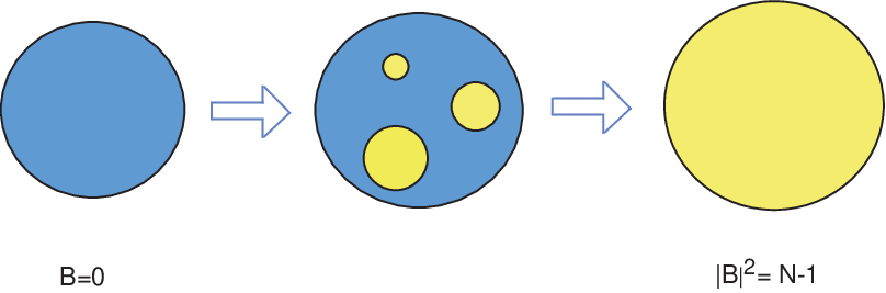
A hint for a possible resolution of the puzzle comes from the idea of the “hole vortex” discussed in [1]. In the case of theory (hence the case of nonAbelian vortex with global color-flavor locked symmetry), part of the zeromodes is the vortex deformation-translational modes, which connect the coaxial vortices all in the same orientation to far-separated singly wound vortices. The onset of such a transition was shown to be characterized by the formation of the vacuum bubble inside the vortex bag, see Fig. 3. Such a hole vortex solution - a sort of mixed phase configuration - was explicitly constructed in [1].
The transition from to vortices in the large winding limit may occur in a similar fashion, through the formation of “bubble vortices” inside the vortex. (Fig. 4).

5 Discussion
Generalizing our previous analysis we studied in the first part of this paper the structure of the nonAbelian BPS vortices in the fully gauged theory, with scalar fields in a bifundamental representation. We have been able to determine explicitly the vortex configurations and gauge field mixing, thanks to the fact that the vortex equations reduce to algebraic equations in the large winding limit. This allowed us to determine exactly all the vortex zeromodes. In the case the right group is global, , our vortex reduces to the well-understood nonAbelian vortices with orientational moduli. The counting in the large winding limit shows that the dimension of the vortex moduli space in the fully gauged theory remains the same, , as in the theory.
Considering the limit of far separated minimally wound vortices, we conclude that the moduli space dimension for each of them is : consistent with a orientational moduli plus translation for each. This is the same as in the systems in which the right global symmetry.
Nevertheless physics of the two systems ( and ) appear to be remarkably different. In the former case the system enjoys a very nontrivial quantum dynamics, which carry on the renormalization group flow below the vortex mass scale, , even though the nontrivial physics now takes place in the subspace of the vortex world sheet. The bulk is in a completely Higgsed phase and has become sterile, below the vortex mass scale.
At the moment the right gauge coupling is turned on, there appear nontrivial unbroken massless gauge fields, coupled to the massless orientational modes. Physics changes instantly and qualitatively. To illustrate some of these new features, we discussed in the second part of this work how some nonlocal, topological effects make appearance in our systems. Note that these new nonlocal effects are washed away in the former case (), due to the fact that the orientational modes strongly fluctuate at long distances. In other words, the interesting quantum dynamics kills the would-be beautiful nonlocal effects in of the theory. In this sense, the two formally very closely related systems – the theories with and – are actually more complementary than similar.
We have seen that the general theory developed earlier to deal with vortices with a residual gauge invariance in the bulk, basically applies also to our model. At the same time, our model presents some interesting features that are new with respect to the specific examples which were treated in the existing literature. Our nonAbelian vortex system is rather special in that the unbroken group is both continuous and nonAbelian. Each vortex is labeled by an element which further breaks . The vortex moduli space contains a orientational moduli. We have shown that the effect of such vortex orientational modes is physical, in spite of the fact that they arise from the breaking of the gauge symmetry by the vortices, and visible at large distances as global topological effects such as the AB scattering. This is a particular type of nonAbelian AB effect. As discussed in some cases earlier, phenomena such as vortex-vortex scattering, topological obstruction, Cheshire charge, and nonAbelian statistics are all present.
More dynamical aspects of zeromode excitations of our systems and the properties of the low-energy effective actions, will be discussed in a separate work.
Acknowledgments
We thank Roberto Auzzi, Jarah Evslin, Simone Giacomelli, Muneto Nitta and Keisuke Ohashi for discussions. The work of SB is funded by the grant “Rientro dei Cervelli Rita Levi Montalcini” of the Italian government. This work is supported by the INFN special research project, “Gauge and String Theories” (GAST).
References
- [1] S. Bolognesi, C. Chatterjee, S. B. Gudnason and K. Konishi, “Vortex zeromodes, Large Flux Limit and Ambjørn-Nielsen-Olesen Magnetic Instabilities,” arXiv:1408.1572 [hep-th].
- [2] S. Bolognesi, “Domain walls and flux tubes,” Nucl. Phys. B 730, 127 (2005) [arXiv:hep-th/0507273], “Large N, Z(N) strings and bag models, ” Nucl. Phys. B 730, 150 (2005) [arXiv:hep-th/0507286].
- [3] S. Bolognesi and S. B. Gudnason, “Multi-vortices are wall vortices: A Numerical proof,” Nucl. Phys. B 741 (2006) 1 [hep-th/0512132].
- [4] R. Auzzi, S. Bolognesi, J. Evslin, K. Konishi and A. Yung, “NonAbelian superconductors: Vortices and confinement in N=2 SQCD,” Nucl. Phys. B 673 (2003) 187 [hep-th/0307287].
- [5] A. Hanany and D. Tong, “Vortices, instantons and branes,” JHEP 0307 (2003) 037 [hep-th/0306150].
- [6] M. Shifman and A. Yung, “NonAbelian string junctions as confined monopoles,” Phys. Rev. D 70 (2004) 045004 [hep-th/0403149].
- [7] N. K. Nielsen and P. Olesen, “An Unstable Yang-Mills Field Mode,” Nucl. Phys. B 144 (1978) 376.
- [8] J. Ambjorn and P. Olesen, “On Electroweak Magnetism,” Nucl. Phys. B 315 (1989) 606.
- [9] J. Ambjorn and P. Olesen, “A Condensate Solution Of The Electroweak Theory Which Interpolates Between The Broken And The Symmetric Phase,” Nucl. Phys. B 330 (1990) 193.
- [10] N. S. Manton and N. A. Rink, “Vortices on Hyperbolic Surfaces,” J. Phys. A 43 (2010) 434024 [arXiv:0912.2058 [hep-th]].
- [11] P. Sutcliffe, “Hyperbolic vortices with large magnetic flux,” Phys. Rev. D 85 (2012) 125015 [arXiv:1204.0400 [hep-th]].
- [12] M. Eto, T. Fujimori, M. Nitta and K. Ohashi, “All Exact Solutions of Non-Abelian Vortices from Yang-Mills Instantons,” JHEP 1307, 034 (2013) [arXiv:1207.5143 [hep-th]].
- [13] M. G. Alford, K. Benson, S. R. Coleman, J. March-Russell and F. Wilczek, “Zeromodes of nonabelian vortices,” Nucl. Phys. B 349 (1991) 414.
- [14] M. G. Alford, K. Benson, S. R. Coleman, J. March-Russell and F. Wilczek, “The Interactions and Excitations of Nonabelian Vortices,” Phys. Rev. Lett. 64 (1990) 1632 [Erratum-ibid. 65 (1990) 668].
- [15] M. G. Alford, K. M. Lee, J. March-Russell and J. Preskill, “Quantum field theory of nonAbelian strings and vortices,” Nucl. Phys. B 384 (1992) 251 [hep-th/9112038].
- [16] H. K. Lo and J. Preskill, “NonAbelian vortices and nonAbelian statistics,” Phys. Rev. D 48 (1993) 4821 [hep-th/9306006].
- [17] K. Konishi, M. Nitta and W. Vinci, “Supersymmetry Breaking on Gauged NonAbelian Vortices,” JHEP 1209 (2012) 014 [arXiv:1206.4546 [hep-th]].
- [18] F. Canfora and G. Tallarita, “Constraining Monopoles by Topology: an Autonomous System,” JHEP 1409 (2014) 136 [arXiv:1407.0609 [hep-th]], “ BPS Monopoles in ,” arXiv:1502.02957 [hep-th].
- [19] M. Bucher and A. Goldhaber, “SO(10) Cosmic strings and SU(3)-color Cheshire charge,” Phys. Rev. D 49 (1994) 4167 [hep-ph/9310262].
- [20] J. Evslin, K. Konishi, M. Nitta, K. Ohashi and W. Vinci, “NonAbelian Vortices with an Aharonov-Bohm Effect,” JHEP 1401, 086 (2014) [arXiv:1310.1224 [hep-th]].