Effect of randomness in logistic maps
Abstract
We study a random logistic map where are bounded (), random variables independently drawn from a distribution. does not show any regular behaviour in time. We find that shows fully ergodic behaviour when the maximum allowed value of is . However , averaged over different realisations reaches a fixed point. For the system shows nonchaotic behaviour and the Lyapunov exponent is strongly dependent on the asymmetry of the distribution from which is drawn. Chaotic behaviour is seen to occur beyond a threshold value of () when () is varied. The most striking result is that the random map is chaotic even when is less than the threshold value at which chaos occurs in the non random map. We also employ a different method in which a different set of random variables are used for the evolution of two initially identical values, here the chaotic regime exists for all values.
pacs
05.45.-a,05.90.+m,87.23,74.40.DeI Introduction
Many natural phenomena show chaotic behaviour and a possible route to chaos is provided by nonlinear dynamical models. In the study of nonlinear dynamics, logistic map is a well known area of research [1]. Study of logistic map is relevant in population dynamics [2], image encryption [3, 4, 5], electronic circuit, pseudo-random number generators [6, 7] etc. Mathematically, the logistic map is given by
| (1) |
The logistic map is perhaps the most simple and illustrative example of iterative maps of the form which shows very complex dynamical behaviour. In this map, for a nonzero steady value is reached. For larger multiple fixed point values with periodicity etc. occur, while above , chaos occurs which is exhibited by a positive Lyapunov exponent [1].
In reality, dynamical phenomena e.g. population dynamics, usually involve an amount of stochasticity. In order to incorporate this feature, we analyse the behaviour of the logistic map where does not have a fixed value but is a random variable , drawn independently from a distribution. In some earlier works [8, 9, 10], such randomisation of has been considered where the main issue was to check whether as such that the distribution of at large times is a delta function at . It was concluded that under certain condition this is true.
We use different distributions for choosing the control parameter . We choose to be bounded, i.e., with to avoid the fixed point as obtained in the earlier cases [9, 8, 10].
We study the behaviour of the quantity defined as
| (2) |
where and denote the two different evolutions. is the average value obtained from different configuration as denoted by the angular brackets on the right hand side of (2). The evolution has been implemented in two different ways: in the traditional method (TM), one starts with two initially close values and to calculate as these two initial values are evolved using the same set of . In the other method, different sets of are used for initially identical values of . The latter is called the “Nature vs. nurture” method following [11].
As usual, if grows (or saturates at a finite value as it cannot increase indefinitely) we conclude that the chaotic regime is reached. Varying and we identify such regions in both the methods. Apart from identifying the chaotic region, we are also interested in comparing the TM and NVN methods which have led to different results in interacting dynamical systems [11, 12].
One of the main objectives is to study whether universal behaviour is observed when we vary the distribution. For this purpose, we have used a uniform distribution and a triangular distribution which has a peak at a value (), from which the values are chosen. For the triangular distribution signifies a symmetric triangular distribution. Deviation of from this value quantifies the asymmetry.
In the next two sections we discuss the results and in section IV summary and discussions are presented.
II Ergodicity and convergence
We first report some general results which are in stark contrast to the non-random map. We use either a uniform distribution or a symmetric triangular distribution for these studies.
Let the initial value of be chosen randomly from [:]. In the non-random logistic map, it is known that has finite number of attractors in the nonchaotic regime. In the random case however has an ergodic type behaviour in the sense that it does not reach a fixed attractor and can assume values between and ; is nonzero for . When is fixed at , shows an increasing behaviour with . However when , for any value of showing that the system becomes fully ergodic (fig. 2). The fate of two independent evolutions depends on and ; however we note that the average value of all such evolution shows convergence and is non ergodic.

It is known that for a fixed value of , the non-random logistic map has a fixed point at which is stable below . For the random case, one can approximate theoretically,
| (3) |
where denotes the average value. If we allow the distribution of to vary between and , we find that the value of obtained numerically differs from obtained using eq. 3 (Table 1). We have shown that while the non ergodicity behaviour is present for both the uniform and symmetric triangular distribution, the deviation of is larger for the uniform distribution compared to that in the symmetric triangular distribution from . Also, ( increases with in the uniform distribution. However, this increase appears to be weaker in case of the symmetric triangular distribution.

III Results for TM method
III.0.1 Non-chaotic regime
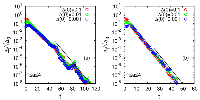
We choose a pair of initial values of which are slightly different and allow them to evolve as a function of time (eq. 2). Typical evolutions for and of two initially close values are shown in figs. 1a, 1b. Although does not attain a fixed point value, we find that indeed goes to zero in an exponential manner for chosen values of and (e.g. for ; see figs. 3a, 3b) signifying regular or nonchaotic behaviour. However, here we find that varies in a nonlinear manner with ; precisely, , whereas for non-random logistic map it is . The Lyapunov exponent depends strongly on ; it shows an increase as is decreased. The value of the Lyapunov exponent is for uniform distribution for
has been studied for asymmetric triangular distribution for (Fig. 3c). Here the Lyapunov exponent remains constant upto and decreases with for higher values (Fig. 3d). This signifies that as increases, vanishes in a slower manner.
| Distribution | Theor. value | Actual value |
|---|---|---|
| Uniform, | ||
| Uniform, | ||
| Symmetric triangular, | ||
| Symmetric triangular, |

III.0.2 Chaotic regime
When is a variable and , as for any value of . However increasing , we note that may reach a nonzero value, e.g, when and signifying a chaotic behaviour. Typical evolutions for and of two initially close values are shown in figs. 4a, 4b. In this case, the damage saturates to a nonzero value (Figs. 4c, 4d main plot). We have used here either a uniform distribution or a symmetric triangular distribution for . Saturation value of the damage has been studied for both the distributions for different values of and . One can keep variable and fix and observe the onset of chaos at a threshold value of (Fig. 5 upper panel). Calling this threshold value , we note that is a function of and decreases with which is expected. This is true for both distributions (Fig. 5 upper panel inset). We note that the minimum value of for the onset of chaos is for the uniform distribution and for the symmetric triangular distribution. Even for , where is the threshold value for onset of chaos in the non random map, one can observe a chaotic region for both the distributions.


Similarly one can keep variable and fix and observe the onset of chaos at a threshold value of (Fig. 5 lower panel). Calling this threshold value , we again note that it is a function of (Fig. 5 lower panel inset). What is striking is the presence of a peak at around which is very close to . It is found that for , the minimum value of required for chaos is . Note that this is the value above which bifurcations start occurring in the nonrandom map. In fact for , the threshold value is weakly dependent on and remains in the entire region. Above , however, smaller values of allow chaos.


IV Results for the NVN Method
We next discuss the results for the NVN method. In this case, two copies of , initially identical, evolve independently, i.e., using different random numbers drawn from identical distributions. Here also the control parameter is chosen from uniform and symmetric triangular distributions. We find that independent of the values of and , the time evolved values of the two copies never converge as long as . Both copies evolve with different values at all times (Fig. 6); however, the configuration average of course is the same as that in the TM case.
The damage as a function of time initially increases and then takes a steady value. The saturation value of is nonzero for all the different regions of control parameter (Fig. 7) as is expected from the evolution of . This is again true for both the distributions.


The saturation value of the damage has been studied. When is fixed and the upper limit is varied (), the value of increases with right from as there is no threshold value of the chaos (Figs. 8a, 8b).
If we keep as a variable () and fixed, the saturation value shows an interesting behaviour. Up to , it decreases with . At a critical value of , it shows a non-monotonic behaviour, with a sharp rise close to before decreasing to zero at . Beyond this critical value of , the initial decrease in becomes less prominent and it increases right up to indicating there is a sharp discontinuity of at (Figs. 8c, 8d). This behaviour is like that in TM (Fig. 5 main plot), however the difference is, one has an onset of chaos in TM such that increases from zero while in NVN, it increases from a nearly constant non-zero value.


One can estimate the maximum possible value of assuming two completely uncorrelated maps as:
where , denote distribution of and . Assuming and to be uniform, . Therefore the expected value of for uncorrelated maps. is indeed less than for both NVN and TM.
V Summary and discussion
In summary, we have studied the behaviour of random logistic maps where the parameter in eq. 1 is a random variable. shows semi or fully ergodic behaviour for such maps, however attains saturation values which differ from the theoretical mean field values as given by eq. 3. The deviations are less in case of a symmetric triangular distribution as it has less variance (Table I).
It is known that randomness in linear systems may give rise to chaos [13]. In the present model, we can identify nontrivial nonchaotic behaviour even with both randomness and nonlinearity. In the nonchaotic regime we find the unconventional behaviour ). Here, one can estimate the Lyapunov exponent . We observe that shows nonuniversality in the sense it shows strong dependence on the asymmetry of the distribution which may be quantified by .
Onset of chaos is noted in the traditional method at threshold values of () which are dependent on (). Minimum values for onset of chaos is found to be (for the uniform distribution) and (for symmetric triangular distribution) when . On the other hand, for , the corresponding minimum value is with for both the distributions. The most striking result is even when , we obtain chaotic region for for both the distributions (Fig. 5).
In NVN, no threshold values of , are obtained. Chaos occurs for all . However shows interesting variation with and (Fig. 8). In general, increases as increases but is not trivially dependent on and hence we conclude that is a nontrivial function of both and .
Although the maps are random, certain effects of the nonrandom maps seem to be present in the TM results, e.g., the peak of occurs at and minimum value of for is where bifurcation starts occurring in the non random case. Another point that needs to be mentioned is that it has not been possible to estimate Lyapunov exponents in the chaotic regime as saturation values are attained within very short times.
As had been observed earlier [11, 12], the TM and NVN methods yield completely different results. As in the case of damage spreading in opinion dynamics model [12], here too we find that the chaotic regime is obtained for any nonzero value of in the NVN method.
Acknowledgements: AK acknowledges financial support from UGC sanction no. UGC/960/JRF(RFSMS). PS acknowledges financial support from CSIR project.
References
- [1] S. H. Strogatz, Nonlinear Dynamics and Chaos, Perseus Books Publishing (1994).
- [2] R. H. May, Nature 261 459-467 (1976).
- [3] M.S. Baptista, Phys. Lett. A 240 50 (1998).
- [4] W-k. Wong, L-p. Lee and K-w Wong, Computer Physics Communications 138 234-236 (2001).
- [5] N.K. Pareek, V. Patidar and K.K. Sud, Image and Vision Computing 24 926 (2006).
- [6] S. C. Phatak and S. S. Rao, Phys. Rev. E 51 (1995).
- [7] V. Patidar and K. K. Sud, Informatica 33 441 (2009).
- [8] J-F. Chamayou and G. Letac, Journal of Theoretical Probability 4 3 (1991).
- [9] R. N. Bhattacharya and B. V. Rao, in Stochastic processes: A festscrift in honour of Gopinath Kallianpur, Springer-Verlag, p 13-21 (1993).
- [10] D. Steinsaltz, The Annals of Probability 27 1952 (1999).
- [11] J. Ye, J. Machta, C. M. Newman, and D. L. Stein, Phys. Rev. E 88 040101 (2013)
- [12] A. Khaleque and P. Sen, Physica A 413 599 (2014).
- [13] L. Yu, E. Ott and Q. Chen, Phys. Rev. Lett. 65 2935 (1990)