Saari’s homographic conjecture for general masses in planar three-body problem under Newton potential and a strong force potential

In 1969, Donald Saari [18] gave a conjecture;

Some people tried to prove this conjecture more than 30 years without any positive results. However, the discovery of the figure-eight solution in 2000 by Chenciner and Montgomery [2] in the three-body problem under Newton potential make us attend to this conjecture because this solution has almost constant moment of inertia but is not a relative equilibrium.

First successful achievement was made by Christopher McCord [13] in 2004. He proved this conjecture for equal masses case in planar three-body problem under Newton potential ($\alpha=1$). Finally, in conference “Saarifest 2005” held at Guanajuato, Mexico, Richard Moeckel [14, 15] proved this conjecture for three-body problem with general masses in any spacial dimension greater than or equal to 2.

Saari’s original conjecture was generalised to homogeneous potentials given by (2).

The harmonic oscillator $\alpha=-2$ is excluded, because there are trivial counter examples for this potential. Actually, we can simply construct motions with constant moment of inertia while each body moves on each ellipse. For example, $\bi{q}_{k}=(a_{k}\cos(\omega t),b_{k}\sin(\omega t))$, $\omega^{2}=\sum m_{k}$ at the centre of mass frame is a solution of the equation of motion for $\alpha=-2$. Then, the parameters that satisfy $\sum m_{k}a_{k}^{2}=\sum m_{k}b_{k}^{2}=c=$ constant makes $I=c$.

In 2006, Gareth E. Roberts [17] found a counter example of this conjecture in the strong force potential ($\alpha=2$). The figure-eight solution in the strong force potential ($\alpha=2$) is also a counter example. These two motions have constant moment of inertia but is not a relative equilibrium. This exceptional behaviour of the $N$-body problem in $\alpha=2$ was already pointed out by Alain Chenciner [1] in 1997. Actually, he noticed that the Lagrange-Jacobi identity for $\alpha\neq 0$ yields

Therefore, $I=$ constant makes $U=$ constant for $\alpha\neq 2$, while $U$ can vary in time for $\alpha=2$. For $\alpha=2$, integrating $d^{2}I/dt^{2}=4E$, we get $I=2Et^{2}+c_{1}t+c_{2}$ with constant parameter $c_{1}$ and $c_{2}$. So, any motion with initial condition $E=0$ and $c_{1}=0$ has constant moment of inertia.

One more known counter example for generalised Saari’s conjecture is rectilinear motion in the equal mass three-body problem under the potential $\alpha=-4$ that was described in the section 1. For this case, $U=-9I^{2}/8$ is an identity. Therefore, $\partial U/\partial x_{i}=-(9I/2)x_{i}$ makes any motion with constant $I$ a harmonic oscillation, which is rectilinear not a relative equilibrium rotation [6].

In the next day of the same conference where Moeckel proved Saari’s original conjecture for three-body problem, Saari gave a talk and extended his conjecture in another way [19, 20], which is the conjecture 1.

Saari’s homographic conjecture is actually an extension of original and generalised conjecture. Indeed, for $\alpha\neq 2$, $I=$ constant makes $U=$ constant, thus makes $\mu=\alpha I^{\alpha/2}U=$ constant. So, Saari’s homographic conjecture contains original conjecture and generalised conjecture for $\alpha\neq 2$. We expect that this conjecture is true for all $\alpha\neq-2,-4$.

The counter example of Roberts and figure-eight solution both in $\alpha=2$ has constant $I$ and non-constant $U$, therefore non-constant $\mu$. So, these two examples do not satisfy the assumption of the homographic conjecture. Therefore, they are not the counter example for this conjecture. We expect that Saari’s homographic conjecture is true for $\alpha=2$. Actually, in this paper, we will prove the conjecture for $\alpha=2$ in planar three-body problem with general masses.

On the other hands, the potential for $\alpha=-2,-4$ are really exceptions for Saari’s homographic conjecture, because $\mu$ is identically equal to a constant value in these potentials.

Florin Diacu, Ernesto Pérez-Chavela, and Manuele Santoprete [4] in 2005 proved this conjecture for collinear $N$-body problem for any $\alpha$. Florin Diacu, Toshiaki Fujiwara, Ernesto Pérez-Chavela and Manuele Santoprete [5] in 2008 showed that the conjecture is true for many set of initial conditions for planar three-body problem. In this paper [5], the authors call this conjecture “Saari’s homographic conjecture” to distinguish this conjecture from similar two other “Saari’s conjecture”. The present authors in 2012 proved the conjecture for planar equal-mass three-body problem under the strong force potential [7] and under Newton potential [8]. In this paper, we extend our proof to general masses case.

In this paper, we consider the planar three-body problem. We identify a two dimensional vector $\bi{a}=(a_{x},a_{y})\in\mathbb{R}^{2}$ and a complex number $a=a_{x}+ia_{y}\in\mathbb{C}$. Inner and outer products are defined by $a\cdot b=a_{x}b_{x}+a_{y}b_{y}$ and $a\wedge b=a_{x}b_{y}-a_{y}b_{x}$. The partial differentiation by $a$ is defined

For example, for $|a|^{2}=a_{x}^{2}+a_{y}^{2}$, $\partial|a|^{2}/\partial a=2(a_{x}+ia_{y})=2a$.

We take the centre of mass frame. So the position vectors $q_{k}$ always satisfy

and the moment of inertia is expressed by $I=\sum m_{k}|q_{k}|^{2}$.

According to Richard Moeckel and Richard Montgomery [16], we define the “shape variable” $\zeta\in\mathbb{C}$ by the ratio of two Jacobi vectors $J_{1}$ and $J_{2}$,

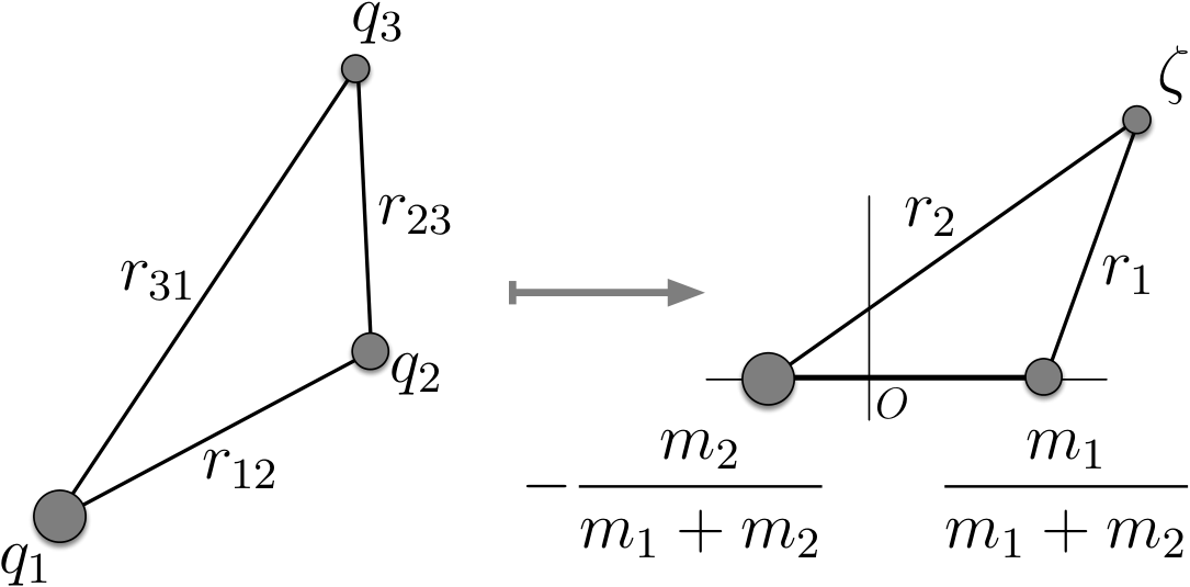
The variable $\zeta$ has a simple geometric interpretation. Consider a similarity transformation that involves a parallel transformation

The points $q_{1}$, $q_{2}$ are mapped to fixed points

then the image of $q_{3}\mapsto\zeta$ represents the shape of the triangle. See figure 1. It is convenient to use the following rescaled “shape variable” $\eta$ instead of $\zeta$,

Let us define $\xi_{k}=q_{k}/(q_{2}-q_{1})$ that satisfy $\xi_{2}-\xi_{1}=1$ and $m_{1}\xi_{1}+m_{2}\xi_{2}+m_{3}\xi_{3}=0$. Explicit expression for $\xi_{k}$ by $\eta$ is

Obviously, the triangles made by $\{q_{k}\}$ and by $\{\xi_{k}\}$ are similar with the common centre of mass. Therefore, there are $r\geq 0$ and $\phi\in\mathbb{R}$, such that

We take the variables $r$, $\phi$ and $\eta$ as the dynamical variables.

The moment of inertia (3) is given by

The kinetic energy is expressed by the variables $r$, $\phi$ and $\eta$,

where dots placed over variables represent the derivative with respect to time. The terms of the right-hand side of (18) represent the kinetic energy for the size motion, for the rotation and for the motion in shape respectively. The potential function (2) for $\alpha\neq 0$ is expressed as

Thus, we obtained expressions for the kinetic energy (18), the potential function (19), and thus the Lagrangian $L$ and the total energy $E$ are represented by the variables $r$, $\phi$ and $\eta$.

Since the variable $\phi$ is cyclic, the angular momentum $C$ is constant of motion.

The equation of motion for $r$ is

Multiplying both sides of (21) by $\dot{r}$, we obtain

Then, using this equation and the energy conservation $dE/dt=0$, we obtain the following relation which was first derived by Saari [20],

This equation shows that the variation in $\mu$ is proportional to the variation in the kinetic energy of the shape motion multiplied by $r^{2}$. Let us define $v^{2}$ as

Then the total energy is given by

and $v=$ constant if and only if $\mu=$ constant. Inspired by Saari’s relation, let us introduce a new “time” variable $\tau$ by

The equation of motion for $\eta$ in the time variable $\tau$ is

Now, consider a motion that has a constant value of $\mu$. Then, by Saari’s relation, the motion must have constant value of $v^{2}$. We have two cases.

For homographic motion, the equation of motion (27) demands that the shape variable must satisfy $\partial\mu/\partial\eta=0$. We know five solutions: two Lagrange configurations and three Euler configurations.

Since such motion satisfy

the “velocity” in the shape variable $d\eta/d\tau$ must be orthogonal to the gradient vector $\partial\mu/\partial\eta$ and must have the magnitude $v$. Therefore, the “velocity” is uniquely determined by the gradient vector and $v$,

Here, $v\in\mathbb{R}$ and $v\neq 0$. In the $\eta$ plane, the motion may pass through a critical point $\partial\mu/\partial\eta=0$. However, we assume a motion with finite $v$ and the critical point is discrete. Therefore, we can find a part of motion with finite length where $\partial\mu/\partial\eta\neq 0$. In the following arguments, we assume $\partial\mu/\partial\eta\neq 0$ without loss of generality.

Does this motion satisfy the equation of motion? To give an answer we calculate the component of the acceleration $d^{2}\eta/d\tau^{2}$ in the orthogonal component to the velocity $d\eta/d\tau$, because parallel component to the velocity is always zero both in the equation of motion (27) and in the motion (30). From the velocity (30) and its derivative by $\tau$, using $d/d\tau=d\eta/d\tau\cdot d/d\eta$, we obtain

where $x,y\in\mathbb{R}$ is defined by $\eta=x+iy$ and $\mu_{x}=\partial\mu/\partial x$, $\mu_{y}=\partial\mu/\partial y$, etc…. On the other hand, the equation of motion and the velocity (30) yields

Two expressions in (31) and (32) must be the same. Thus, we get a necessary condition that must be satisfied by a non-homographic motion with constant $\mu$,

The right-hand side of the necessary condition is written in the Cartesian coordinate $(x,y)$. It is convenient to write the right-hand side in a coordinate free form. The kinetic energy for the shape motion in the equation (18) naturally defines the distance squared $ds^{2}$ and the metric tensor $g_{ij}$ as follows,

Here the repeated indices are understood to be summed. The vector $(dx^{1},dx^{2})$ is identified to be $(dx,dy)$ and $\delta_{ij}$ represents the Kronecker symbol,

This metric space is called “Shape Sphere”. This sphere is exactly the Riemann sphere of the complex plane $x+iy$. This fact was first noticed by George Lemaître [12] and used by Hsiang and Straume [9, 10], Chenciner and Montgomery [2], Montgomery and Mockel [16], Kuwabara and Tanikawa [11].

The inverse and the determinant of the metric are

Let us define the following three scalars,

In each equality, the first step is definition of each scalar, and the last step is a representation in $(x,y)$ coordinates. The derivative with respect to time $t$ is given by

Where, $D$ is a differential operator defined by

and $\epsilon^{ij}$ is the Lévi-Cività anti-symmetric symbol

Using these scalars, the necessary condition (33) is written in the coordinate free expression,

In this section, we will show a method to rewrite the necessary condition (43) in the two-center bipolar coordinates defined by

See figure 1. Although the coordinates $\eta=x+iy=\sqrt{n}\,\zeta$ are useful to describe the Lagrangian and to get the equations of motion, they are not convenient to express the necessary condition. The expression of the condition in $(x,y)$ coordinates is lengthy and complex, while in $r_{1}$ and $r_{2}$ is relatively short and simple.

In the variables $x$ and $y$,

Inversely,

Then, distance squared $ds^{2}=(dx^{2}+dy^{2})/(1+x^{2}+y^{2})^{2}$ is given by

Then the metric tensor for this coordinates is defined by

with $a=r_{1}r_{2}$ and $b=-(r_{1}^{2}+r_{2}^{2}-1)/2$. The inverse metric $g^{ij}$ and $|g|^{1/2}$ are

Using $\mu$ for $\alpha\neq 0$ expressed as functions of $r_{\ell}$, $\ell=1,2$,

three scalars (37)–(39) and thus necessary condition (43) are expressed as a function of $r_{l}$.

For the strong force potential $\alpha=2$, the left-hand side of the necessary condition (43) is constant and the right-hand side is a function of $r_{\ell}^{2}$,

Two variables $r_{1}^{2}$ and $r_{2}^{2}$ are not independent, because we are considering a motion that has $\mu(r_{1}^{2},r_{2}^{2})=$ constant. We have only one independent variable. See figure 2.

A possible choice of one independent variable is, say, $r_{1}^{2}$. Solving $\mu(r_{1}^{2},r_{2}^{2})=\mu$ for $r_{2}^{2}$, we will obtain $r_{2}^{2}=r_{2}^{2}(m_{k},\mu,r_{1}^{2})$. Then, the necessary condition (54) will be in the form $1/2=F(m_{k},C,v,\mu,r_{1}^{2})$. This is a condition for independent variable $r_{1}^{2}$ with constants $m_{k},C,v,\mu$. However, this choice breaks the invariance of the condition (54) under the simultaneous exchange of $m_{1}\leftrightarrow m_{2}$ and $r_{1}^{2}\leftrightarrow r_{2}^{2}$. Breaking this symmetry will make our analysis complex. Let us write a desirable variables $\{\nu,\rho\}$ that would keep this symmetry, easy to solve the variable change $\{r_{1}^{2},r_{2}^{2}\}\leftrightarrow\{\nu,\rho\}$, and simple to eliminate one variable using $\mu=$ constant.

Our choice for $\{\nu,\rho\}$ is

Obviously, these variables keep the symmetry. The equation (55) is easy to solve for $\{r_{1}^{2},r_{2}^{2}\}$ because this equation is quadratic. Moreover, we simply eliminate $\nu$ by

We have two solutions of $r_{\ell}^{2}=r_{\ell}^{2}(\tilde{\mu},\rho)$ for the equation (55). Substituting a solution into the necessary condition (54), we obtain a necessary condition for $\rho$ as follows,

Now, if there is a non-homographic motion with constant $\mu=\tilde{\mu}/(m_{1}+m_{2}+m_{3})$, there is some finite physical interval of $\rho$ where the condition (57) is satisfied. See figure 2. Since the right-hand side of the condition (57) is an analytic function of $\rho$, this condition must be satisfied for whole complex plane of $\rho\in\mathbb{C}$. Therefore, the condition (57) must be satisfied near the origin of $\rho$, although this region is unphysical.

Two solutions of (55) are

and

References

- [1]
Chenciner A, 1997
Introduction to the N-body problem,
Preprint http://www.bdl.fr/Equipes/ASD/preprints/prep.1997/Ravello.1997.pdf - [2] Chenciner A and Montgomery R, 2000 A remarkable periodic solution of the three-body problem in the case of equal masses, Ann. Math. 152, 881–901
- [3] Chenciner A, 2003 Some facts and more questions about the Eight, Topological Methods, Variational Methods and Their Applications, Proc. ICM Satellite Conf. on Nonlinear Functional Analysis (Taiyuan, China, 1418 August 2002) (Singapore: World Scientific) pp 77-88
- [4] Diacu F, Pérez-Chavela E, and Santoprete M, 2005, Saari’s conjecture of the N-body problem in the collinear case, Trans. Amer. Math. Soc. 357, 4215–4223
- [5] Diacu F, Fujiwara T, Pérez-Chavela E and Santoprete M, 2008, Saari’s homographic conjecture of the three-body problem, Transactions of the American Mathematical Society, 360, 12, 6447–6473
- [6] Fujiwara T, Fukuda H, and Ozaki H, 2003, Evolution of the moment of inertia of three-body figure-eight choreography, J. Phys. A: Math. Gen. 36 10537–10549
- [7] Fujiwara T, Fukuda H, Ozaki H, and Taniguchi T, 2012, Saari’s homographic conjecture for planar equal-mass three-body problem under a strong force potential, J. Phys. A: Math. Theor. 45 045208
- [8] Fujiwara T, Fukuda H, Ozaki H, and Taniguchi T, 2012, Saari’s homographic conjecture for a planar equal-mass three-body problem under the Newton gravity, J. Phys. A: Math. Theor. 45 345202
- [9] Hsiang W Y and Straume E, 1995, Kinematic geometry of triangles with given mass distribution, PAM-636Report (Berkeley, CA: University of California)
- [10] Hsiang W Y and Straume E, 2006, Kinematic geometry of triangles and the study of the three-body problem, arXiv:math-ph/0608060
- [11] Kuwabara K H and Tanikawa K, 2010, A new set of variables in the three-body problem, Publ. Astron. Soc. Japan 62 1–7
- [12] Lemaître G, 1955, Regularization of the three-body problem, Vistas in Astronomy, 1, 207–215
- [13] McCord C, 2004, Saari’s conjecture for the planar three-body problem with equal masses, Celestial Mechanics, 89, 2, 99–118
- [14] Moeckel R, 2005, Saari’s conjecture in , Presentation at Saarifest 2005, April 7, 2005, Guanajuato, Mexico.
- [15] Moeckel R, 2005, A computer assisted proof of Saari’s conjecture for the planar three-body problem, Transactions of the American Mathematical Society, 357, 3105–3117
- [16] Moeckel R and Montgomery R, 2007, Lagrangian reduction, regularisation and blow-up of the planar three-body problem, preprint
- [17] Roberts G E, 2006, Some counterexamples to a generalised Saari’s conjecture, Transactions of the American Mathematical Society, 358, 251–265
- [18] Saari D, 1970 On bounded solutions of the n-body problem, Periodic Orbits, Stability and Resonances, G.E.O., Giacaglia (Ed.), D. Riedel, Dordrecht, 76–81
- [19] Saari D, 2005, Some ideas about the future of Celestial Mechanics, Presentation at Saarifest 2005, April 8, 2005, Guanajuato, Mexico
- [20] Saari D, 2005, Collisions, rings, and other Newtonian N-body problems, American Mathematical Society, Regional Conference Series in Mathematics, No. 104, Providence, RI